Energy-efficient Resource Allocation for Wirelessly Powered Backscatter Communications

Abstract

In this letter we consider a wireless-powered backscatter communication (WP-BackCom) network, where the transmitter first harvests energy from a dedicated energy RF source ($S$) in the sleep state. It subsequently backscatters information and harvests energy simultaneously through a reflection coefficient. Our goal is to maximize the achievable energy efficiency of the WP-BackCom network via jointly optimizing time allocation, reflection coefficient, and transmit power of $S$. The optimization problem is non-convex and challenging to solve. We develop an efficient Dinkelbach-based iterative algorithm to obtain the optimal resource allocation scheme. The study shows that for each iteration, the energy-efficient WP-BackCom network is equivalent to either the network in which the transmitter always operates in the active state, or the network in which $S$ adopts the maximum allowed power.

I Introduction

The limited battery lifetime of Internet of Things (IoT) devices can become a fundamental problem for massive IoT deployment. Several advanced technologies, e.g, wireless-powered communication networks (WPCNs) [1] and backscatter communications [2], have been proposed to address this problem. One particular promising solution is to use the backscatter communication since it allows IoT devices to modulate and reflect the incident RF signals instead of generating RF signals by itself and to harvest energy for circuit operation. Hence backscatter communications consume much less energy than WPCN involving oscillators, analog-to-digital/digital-to-analog converters [2].

In [3], the hardware of backscatter communication prototypes was designed by leveraging ambient WiFi signals to realize backscatter and energy harvesting. In [4], the authors investigated the impacts of the time allocation and the reflection coefficient on wirelessly powered backscatter communication system (WP-BackComs), where dedicated RF energy sources were deployed to power backscatter users. The coexistence of harvest-then-transmit protocol and backscatter communication was also investigated in wireless-powered heterogeneous networks [5], where ambient RF signals and dedicated RF signals transmitted by a dedicated energy source are considered. In addition to [4, 5], where the main focus was on system-level backscatter communications, the authors of [6] studied the joint design of time allocation and reflection coefficient to maximize throughput in a typical backscatter communication scenario that consists of one RF energy source, one backscatter user, and one receiver. The outage probability was also derived in a similar scenario [7]. Backscatter communication has also been combined with other types of communication techniques, e.g., cognitive radio [8, 9], device-to-device [10], non-orthogonal multiple access [11] and relaying [12, 13]. Other works on the waveform design and detection algorithm design can also be found in [14, 15].

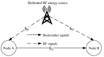
Figure 1: System Model

Although the aforementioned works [3, 15, 4, 5, 6, 7, 8, 9, 10, 14, 12, 13, 11] have laid a solid foundation for understanding backscatter communications from various perspectives, e.g., hardware design and spectral efficiency (SE), the energy efficiency (EE) of backscatter communication has not been studied yet. To the best of our knowledge, this is the first work to consider energy-efficient resource allocation problem in a WP-BackCom network, where the transmitter modulates and reflects its information to the receiver via RF signals from the dedicated RF energy source ($S$), as well as harvests energy to power its circuit. An efficient Dinkelbach-based iterative algorithm is developed to determine the energy-efficient resource allocation scheme. Specifically, an optimization problem is formulated to maximize the EE by jointly optimizing the time allocation, the reflection coefficient, and the transmit power of $S$. The non-convex original optimization problem in the fractional form is transformed into an equivalent problem in the subtractive form based on the fractional programming. The transformed problem can be cast into two convex EE maximization problems. In one problem the transmitter operates in the active state and in the other problem $S$ adopts the maximum allowed power.

II System Model And Working Flow

Fig. 1 shows a WP-BackCom network consisting of one $S$, one transmitter $A$ with backscatter circuits, and one receiver $B$. The nodes $B$ and $S$ have stable energy sources. Node $A$ is a battery-free node and backscatter communication is employed to realize information transfer and harvest energy for circuit operation. The harvested energy in each slot is temporarily stored in a capacitor of node $A$. For simplicity, we assume that part of stored energy is used to power circuits and the rest is fully discharged in the same slot. In other words, there will be no energy stored in node $A$ at the end of each slot. An entire slot is less than the coherence interval, which is normalized to 1 without loss of generality. There are two states, sleep state $\tau_{s}$ and active state $\tau_{a}$, in one slot. Let $h_{0}$, $h_{1}$, $h_{2}$ denote the channel gains of $S-A$ link, the $A-B$ link, and $S-B$ link, respectively. Each link is assumed to undergo independent identically distributed quasi-static fading and to be reciprocal. Motivated by the recent works [4, 5, 11, 6, 7, 8, 9, 10, 12, 13, 14] in this filed, we assume perfect CSI is available to obtain an EE upper bound of a WP-BackCom. The way to obtain $h_{0}$ and $h_{1}$ can be found in [14] and $h_{2}$ can be estimated by the conventional traditional pilot-based method. Relaxing this assumption into imperfect CSI makes our considered network more realistic, which can be studied in our future work.

For each slot, node $A$ leverages the RF signals $x(n)$ $\left({\mathbb{E}\left[{{{\left|{x\left(n\right)}\right|}^{2}}}\right]=1}\right)$ from $S$ to realize information transmission and energy harvesting for circuit operation. Node $A$ firstly operates in the sleep state to harvest energy from received RF signals and the harvested energy in this state is calculated as ${E_{\rm{sleep}}^{h}}=\eta{P_{\rm{0}}}{h_{0}}{\tau_{s}}$, where $P_{0}$ and $\eta$ are the transmit power of $S$ and the energy harvesting (EH) efficiency coefficient , respectively. Here we ignore the harvested energy from the noise since the thermal noise power of the passive node $A$ is much smaller than the received signals $x(n)$ [5, 8, 7, 9, 6]. In the active state, part of the received RF signal, $\sqrt{\beta P_{0}{h_{0}}}x\left(n\right)$, is employed by the vehicle for modulating and backscattering the information of node $A$ and the rest, $\sqrt{(1-\beta)P_{0}{h_{0}}}x\left(n\right)$, is flown into the energy harvester. For convenience, we refer $0\!<\!\beta\!\leq\!1$ as the reflection coefficient [7, 4, 6, 9]. Thus, the harvested energy in this state and the backscattered signals are written as ${E_{\rm{active}}^{h}}=\eta\left({1-\beta}\right){P_{0}}{h_{0}}{\tau_{a}}$ and $\tilde{x}\left(n\right)=\sqrt{\beta{P_{0}}{h_{0}}}x\left(n\right)c\left(n\right)$, respectively, where $c(n)$ is node $A$’s signal satisfying $\mathbb{E}\left[{{{\left|{c\left(n\right)}\right|}^{2}}}\right]=1$ [9]. The received signal at node $B$ is given by $y\left(n\right)=\sqrt{{h_{1}}}\tilde{x}\left(n\right)+\sqrt{P_{0}{h_{2}}}x\left(n\right)+w\left(n\right)$, where $w\left(n\right)$ is the additive white Gaussian noise with variance $\sigma^{2}$ at the receiver. In our work, the energy source $S$ only serves as a RF source and hence the transmitted RF signal $x\left(n\right)$ can be a predefined pattern that node $B$ knows. Once the CSI is obtained by node $B$, $\sqrt{P_{0}{h_{2}}}x\left(n\right)$ can be subtracted in $y(n)$ by using existing digital or analog cancellation techniques. For this reason, the received signal-to-noise ratio (SNR) is calculated as $\gamma=\frac{{\beta{P_{0}}{h_{0}}{h_{1}}}}{{{\sigma^{2}}}}$ after applying successive interference cancellation (SIC) at the node $B$ [9, 7, 6, 13]. Then the throughput is $R={\tau_{a}}{\log_{2}}\left({1+\beta{P_{0}}\lambda}\right)$, where $\lambda={\frac{{{h_{0}}{h_{1}}}}{{{\sigma^{2}}}}}$.

The total energy consumption consists of two parts: the energy consumed in the dedicated energy RF source and the energy consumed in node $B$. Therefore, the total energy consumption of the whole system is written as $E_{{\rm{total}}}^{\rm{c}}=\frac{{{P_{0}}{\tau_{s}}}}{\xi}+P_{sc}\tau_{s}+\frac{{{P_{0}}{\tau_{a}}}}{\xi}+{P_{sc}}{\tau_{a}}+{P_{rc}}{\tau_{a}}$, where $\xi\in\left({0,1}\right]$ is the power amplifier efficiency; $P_{sc}$ and $P_{rc}$ are the constant circuit powers consumed by $S$ and node $B$, respectively. Note that the constant circuit power of node $A$, denoted by $P_{tc}$, is not included in $E_{{\rm{total}}}^{\rm{c}}$ since node $A$ is powered by the harvested energy, which has been included in the energy consumption of the energy RF source $S$.

III Energy-efficient Resource Allocation

III-A Problem Formulation

In this subsection, we formulate an optimization problem to maximize the achievable EE by optimizing the time for sleep and active states, reflection coefficient, and transmit power of $S$. The EE $q$ is defined as the ratio of achievable throughput to the total energy consumption [16], given as $q=\frac{{{\tau_{a}}\log_{2}\left({1+\beta{P_{0}}\lambda}\right)}}{{\frac{{{P_{0}}}}{\xi}\left({{\tau_{a}}+{\tau_{s}}}\right)+{P_{rc}}{\tau_{a}}+{P_{sc}}\left({{\tau_{a}}+{\tau_{s}}}\right)}}=\frac{{\log_{2}\left({1+\beta{P_{0}}\lambda}\right)}}{{\frac{{{P_{0}}}}{\xi}\left({{\rm{1}}+\frac{{{\tau_{s}}}}{{{\tau_{a}}}}}\right)+{P_{rc}}+{P_{sc}}\left({{\rm{1}}+\frac{{{\tau_{s}}}}{{{\tau_{a}}}}}\right)}}$. Thus, the optimization problem is formulated in the following.

$$\begin{array}[]{l}\mathbf{P}_{1}:\mathop{\max}\limits_{{P_{0}},{\tau_{s}},{\tau_{a}},\beta}q\\ \;\;{\rm{s.t}}.\;{\rm{C}}1:0<\beta\leq 1,\;{\rm{C2}}:{\tau_{a}}+{\tau_{s}}=1,\\ \;\;\;\;\;\;\;\;{\rm{C}}3:0<{P_{0}}\leq{P_{\max}},\;{\rm{C4}}:{\tau_{a}>0},{\tau_{s}}\geq 0,\\ \;\;\;\;\;\;\;\;{\rm{C5}}:{P_{tc}}{\tau_{a}}\leq{E_{\rm{sleep}}^{h}}+{E_{\rm{active}}^{h}}.\end{array}$$ (5)

In $\mathbf{P}_{1}$, $\rm{C}3$ constrains the maximum transmit power of $S$. $\rm{C}5$ guarantees that the total energy consumed by node $A$ does not exceed the total harvested energy [6]. Note that the WP-BackCom is different from the conventional relaying and the main differences can be found in [7]. These differences make the formulated EE problem noticeably different from that of the conventional relaying.

Obviously, $\mathbf{P}_{1}$ is a non-convex problem due to the non-convex objective function and the non-convex constraint $\rm{C}5$. In general, there is no standard algorithm to solve non-convex optimization problems efficiently. We propose an iterative algorithm to solve $\mathbf{P}_{1}$ in what follows.

III-B Solution

The problem $\mathbf{P}_{1}$ is a non-linear fractional programming problem and hence this can be solved by developing an efficient Dinkelbach-based iterative algorithm. To this end, Lemma 1 is provided to transfer $\mathbf{P}_{1}$ to a tractable problem.

Lemma 1. The optimal solution of $\mathbf{P}_{1}$ can be obtained if and only if $\mathop{\max}\limits_{{P_{0}},{\tau_{s}},{\tau_{a}},\beta}\log_{2}\left({1+\beta{P_{0}}\lambda}\right)-q\left({\left({\frac{{{P_{0}}}}{\xi}+{{P_{sc}}}}\right)\left({{\rm{1}}+\frac{{{\tau_{s}}}}{{{\tau_{a}}}}}\right)+{P_{rc}}}\right)=\log_{2}\left({1+{\beta^{*}}P_{0}^{*}\lambda}\right)-q\left({\left({\frac{{P_{0}^{*}}}{\xi}+{{P_{sc}}}}\right)\left({{\rm{1}}+\frac{{\tau_{s}^{*}}}{{\tau_{a}^{*}}}}\right)+{P_{rc}}}\right)=0$ holds, where $*$ denotes the optimal solution corresponding to the optimization variables. This Lemma can be proven readily from the generalized fractional programming theory [16].

Based on Lemma 1, the original problem $\mathbf{P}_{1}$ can be solved by solving the following problem $\mathbf{P}_{2}$.

$$\mathbf{P}_{2}: \mathop{\max}\limits_{{P_{0}},{\tau_{s}},{\tau_{a}},\beta}\!\log_{2}\left({1\!+\!\beta{P_{0}}\lambda}\right)\!-\!q\left(\!{\left(\!{\frac{{{P_{0}}}}{\xi}+{{P_{sc}}}}\right)\left({{\rm{1}}+\frac{{{\tau_{s}}}}{{{\tau_{a}}}}}\!\right)+{P_{rc}}}\!\right)$$

$$\;\;\;\;\;{\rm{s}}{\rm{.t}}{\rm{.}}\;\;\rm{C}1-C5.$$ (6)

Even though the problem is more tractable, there are coupling relationships among different optimization variables. Accordingly, the problem $\mathbf{P}_{2}$ is still non-convex. In order to solve it, we first present the following Proposition.

Proposition 1. For any given system parameters and optimization variables, the optimal reflection coefficient ${\beta^{*}}$ of $\mathbf{P}_{2}$ is calculated as ${\beta^{*}}=\max\left\{{0,\min\left\{{1+\frac{{{\tau_{s}}}}{{{\tau_{a}}}}-\frac{{P_{tc}}}{{\eta{P_{0}}{h_{0}}}},1}\right\}}\right\}$.

Proof. Obviously, the objective function of $\mathbf{P}_{2}$ increases with the increase of $\beta$. On the other hand, through some simple mathematical calculations, the constraint $\rm{C}5$ is equivalent to the following inequality, which is $\beta\leq 1+\frac{{{\tau_{s}}}}{{{\tau_{a}}}}-\frac{{P_{tc}}}{{\eta{P_{0}}{h_{0}}}}$. Combining with $\rm{C}1$, the Proposition 1 can be proven.

Remark 1. The proposed Proposition 1 serves two purposes. Firstly, we provide a closed-form expression for the optimal reflection coefficient and hence obtain the optimal reflection coefficient using this expression instead of other iterative algorithms. The second purpose is to obtain insightful understandings on the optimal reflection coefficient. For example, when $0\leq 1+\frac{{{\tau_{s}}}}{{{\tau_{a}}}}-\frac{{P_{tc}}}{{\eta{P_{0}}{h_{0}}}}<1$ holds, the optimal reflection coefficient increases with the increase of $\tau_{s}$, and more power of the (or even all the) received signals in the active state will be used to backscatter, indicating that a higher EE could be achieved; when $1+\frac{{{\tau_{s}}}}{{{\tau_{a}}}}-\frac{{P_{tc}}}{{\eta{P_{0}}{h_{0}}}}\geq 1$ is satisfied, i.e., the harvested energy during sleep state is sufficient to cover the energy consumed by circuits, the transmitter backscatters all the received signals during the active state and assigns more time for the active state and less time for the sleep state for EE maximization.

Based on Proposition 1, $\mathbf{P}_{2}$ is rewritten as

$$\begin{array}[]{l}\mathbf{P}_{3}:\mathop{\max}\limits_{{P_{0}},{\tau_{s}},{\tau_{a}}}\log_{2}\left({k+{P_{0}}\lambda\left({1+\frac{{{\tau_{s}}}}{{{\tau_{a}}}}}\right)}\right)\\ \;\;\;\;\;\;\;\;\;-q\left({\left({\frac{{{P_{0}}}}{\xi}+{P_{sc}}}\right)\left({{\rm{1}}+\frac{{{\tau_{s}}}}{{{\tau_{a}}}}}\right)+{P_{rc}}}\right)\\ {\rm{s}}.{\rm{t}}.\;\;\;\;\;{\rm{C2}}-{\rm{C4}},\;{\rm{C6}}:\;0<1+\frac{{{\tau_{s}}}}{{{\tau_{a}}}}-\frac{{P_{tc}}}{{\eta{P_{0}}{h_{0}}}}\leq 1,\end{array}$$ (10)

where $k=1-{\frac{{\lambda P_{tc}}}{{\eta{h_{0}}}}}$, and $\rm{C}6$ is derived from $\rm{C}1$ and Proposition 1. Observe that the problem $\mathbf{P}_{3}$ has less optimization variables and more tractable compared with the original problem $\mathbf{P}_{2}$. However, the problem $\mathbf{P}_{3}$ is still non-convex due to the existence of coupling in the objection function and the constraint $\rm{C}6$. To cope with it, we introduce two auxiliary variables: $z={P_{0}}\left({1+{{{\tau_{s}}}\mathord{\left/{\vphantom{{{\tau_{s}}}{{(1-\tau_{s})}}}}\right.\kern-1.2pt}{{(1-\tau_{s})}}}}\right)$ and $t={1+\frac{{{\tau_{s}}}}{{{1-\tau_{s}}}}}$. Based on these two auxiliary variables, the problem $\mathbf{P}_{3}$ is equivalent to the following problem, given by

$$\begin{array}[]{*{20}{l}}\mathbf{P}_{4}:{\mathop{\max}\limits_{z,t}\log_{2}\left({k+\lambda z}\right)-q\left({\frac{z}{\xi}+{{P_{sc}}}t+{P_{rc}}}\right)}\\ {{\rm{s}}.{\rm{t}}.\;\;\;}\;{\rm{C}}7:0<z\leq{P_{\max}}t,\\ {\;\;\;\;\;\;\;\;\;{\rm{C}}8:t\geq 1},\;{\rm{C}}9:0<t\left({1-{{P_{tc}}\mathord{\left/{\vphantom{{P_{tc}}{\eta z{h_{0}}}}}\right.\kern-1.2pt}{\eta z{h_{0}}}}}\right)\leq 1,\end{array}$$ (14)

where the constraints $\rm{C}8$ and $\rm{C}9$ are derived from the constraints $\rm{C}4$ and $\rm{C}6$, respectively.

The problem $\mathbf{P}_{4}$ is still non-convex due to the non-convex constraint $\rm{C}9$, while we note that the objective function increases with the decrease of $t$ and the feasible region of $t$ is ${\rm{max}}\{1,{z\mathord{\left/{\vphantom{z{{P_{\max}}}}}\right.\kern-1.2pt}{{P_{\max}}}}\}\leq t\leq\frac{1}{{1-{{P_{tc}}\mathord{\left/{\vphantom{{P_{tc}}{\eta z{h_{0}}}}}\right.\kern-1.2pt}{\eta z{h_{0}}}}}}$. Based on this observation, we show that the problem $\mathbf{P}_{4}$ is equivalent to the following two optimization problems $\mathbf{P}_{5}$ and $\mathbf{P}_{6}$.

$$\begin{array}[]{*{20}{l}}\mathbf{P}_{5}:{\mathop{\max}\limits_{z}\log_{2}\left({k+\lambda z}\right)-q\left({\frac{z}{\xi}+{P_{sc}}+{P_{rc}}}\right)}\\ {{\rm{s}}.{\rm{t}}.\;\;\;{\rm{C10:}}\;0<z\leq{P_{\max}}},{\;{\rm{C11}}:\;\eta z{h_{0}}-{P_{tc}}>0}.\end{array}$$ (17)

$$\begin{array}[]{*{20}{l}}\mathbf{P}_{6}:{\mathop{\max}\limits_{z}\log_{2}\left({k+\lambda z}\right)-q\left({\frac{z}{\xi}+\frac{{z{P_{sc}}}}{{{P_{\max}}}}+{P_{rc}}}\right)}\\ {{\rm{s}}.{\rm{t}}.\;\;\;\;{\rm{C}}12:{P_{\max}}<z},{\;{\rm{C}}13:\frac{{{P_{tc}}}}{{\eta{h_{0}}}}\leq z\leq{P_{\max}}+\frac{{{P_{tc}}}}{{\eta{h_{0}}}}}.\end{array}$$ (20)

$\mathbf{P}_{5}$ and $\mathbf{P}_{6}$ are formulated based on $\frac{z}{{{P_{\max}}}}\leq 1$ and $\frac{z}{{{P_{\max}}}}>1$, respectively. Obviously, the problem $\mathbf{P}_{5}$ (or $\mathbf{P}_{6}$) is convex and can be solved by bisection search method. The computational complexity for $\mathbf{P}_{5}$ (or $\mathbf{P}_{6}$) is $O(\log(\frac{D_{1}}{\varepsilon}))$ (or $O(\log(\frac{D_{2}}{\varepsilon}))$), where ${D_{1}}$ (or $D_{2}$) and ${\varepsilon}$ denote the maximum range of the searching variable and the precision, respectively. If the number of iterations for Algorithm 1 is $K$, the overall computational complexity of Algorithm 1 is $KO(\log(\frac{D_{1}D_{2}}{\varepsilon^{2}}))$, where $D_{1}={P_{\max}}-\frac{{{P_{tc}}}}{{\eta{h_{0}}}}$ and $D_{2}=\min\left\{{{P_{\max}},\frac{{{P_{tc}}}}{{\eta{h_{0}}}}}\right\}$.

Remark 2. If $\frac{z}{{{P_{\max}}}}\leq 1$ holds, we have $t^{*}=1$, $\tau_{s}^{*}=0$ and $\tau_{a}^{*}=1$, indicating that the harvested energy during the active state is sufficient to power the circuit and that node $A$ always operates in the active state. In addition, we derive the closed-form expressions for $z^{*}$ and $P_{0}^{*}$ based on Lagrange duality method and $z^{*}=P^{*}_{0}t^{*}$. $z^{*}=P_{0}^{*}=\frac{{\ln 2}}{{{u_{1}}+{q\mathord{\left/{\vphantom{q\xi}}\right.\kern-1.2pt}\xi}}}-\frac{k}{\lambda}$, where $u_{1}\geq 0$ is a Lagrange multiplier.

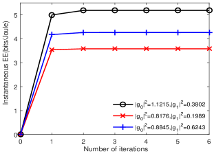
Figure 2: The convergence of Algorithm 1.

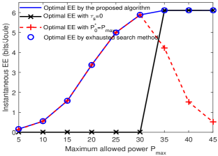
Figure 3: An illustration of Remark 4.

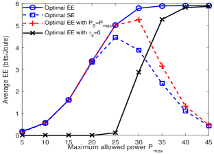
Figure 4: EE versus the maximum allowed power.

Remark 3. If $\frac{z}{{{P_{\max}}}}>1$ is satisfied, we have $t^{*}=\frac{z^{*}}{{{P_{\max}}}}$, $\tau_{s}^{*}>0$ and $0<\tau_{a}^{*}<1$. Combined with $z^{*}=P_{0}^{*}t^{*}$, it is not difficult to find that $P_{0}^{*}=P_{\rm{max}}$. There are two insights: (i) $\tau_{s}^{*}>0$ and $0<\tau_{a}^{*}<1$ mean that ‘sleep-then-active’ is a desirable working mode for node $A$; (ii) the maximum EE could be achieved when the $S$ adopts the maximum allowed power. Moreover, we obtain that ${t^{*}}=\frac{{\ln 2}}{{{{q{P_{\max}}}\mathord{\left/{\vphantom{{q{P_{\max}}}\xi}}\right.\kern-1.2pt}\xi}+{u_{2}}{P_{\max}}-q{P_{sc}}}}-\frac{k}{\lambda}$ by using Lagrange duality method, where $u_{2}\geq 0$ is a Lagrange multiplier. It can be found that $t^{*}$ increases with the increase (decrease) of $P_{sc}$ ($P_{\rm{max}}$). This finding and $t^{*}={1+\frac{{{\tau^{*}_{s}}}}{{{\tau^{*}_{a}}}}}$ reveal the relationships among $\frac{{{\tau^{*}_{s}}}}{{{\tau^{*}_{a}}}}$, $P_{sc}$ and $P_{\rm{max}}$ (or $P^{*}_{0}$).

Remark 4. It can be drawn from remarks 2 and 3 that the problem $\mathbf{P}_{2}$ is equivalent to two optimization problems, $\mathbf{P}_{5}$ and $\mathbf{P}_{6}$, for two simplified sub-systems, which can be obtained by relaxing one constraint, e.g, $\tau_{s}^{*}=0$ or $P^{*}_{0}=P_{\rm{max}}$.

Based on $\mathbf{P}_{2}$$-$$\mathbf{P}_{6}$, we summarize the Dinkelbach-based iterative algorithm for solving $\mathbf{P}_{1}$ in Algorithm 1, where $f_{1}(\cdot)$, $f_{2}(\cdot)$, $z_{1}^{+}$ and $z_{2}^{+}$ denote the objective function of $\mathbf{P}_{5}$, the objective function of $\mathbf{P}_{6}$, the optimal solution of $\mathbf{P}_{5}$ and the optimal solution of $\mathbf{P}_{6}$ in each iteration, respectively. In the proposed Algorithm 1, we solve $\mathbf{P}_{5}$ and $\mathbf{P}_{6}$ instead of $\mathbf{P}_{4}$ with a given $q$ in each iteration and obtain the optimal solution, denoted by $\left({{z^{+}},{t^{+}}}\right)$, by comparing ${f_{1}}\left({z_{1}^{+}}\right)$ with ${f_{2}}\left({z_{2}^{+}}\right)$. For an error tolerance $\epsilon$, the solution to $\mathbf{P}_{4}$ is determined when $\log_{2}\left({k+\lambda{z^{+}}}\right)-\frac{{q{z^{+}}}}{\xi}-q{P_{sc}}{t^{+}}-q{P_{rc}}<\epsilon$ or $l=L_{\max}$ is satisfied.

Algorithm 1 Dinkelbach-based Iterative Algorithm

1:  Set the maximum iterations $L_{\max}$, the maximum error tolerance $\epsilon$, the iteration index $l=0$ and $q=0$.

2:  repeat

3:     Solve $\mathbf{P}_{5}$ and $\mathbf{P}_{6}$ with a given $q$, and obtain the optimal solutions ${{z_{1}^{+}}}$ and ${{z_{2}^{+}}}$;

4:     if ${f_{1}}\left({z_{1}^{+}}\right)>{f_{2}}\left({z_{2}^{+}}\right)$ then

5:        $z^{+}=z_{1}^{+}$ and $t^{+}=1$

6:     else

7:        Set $z^{+}=z_{2}^{+}$ and $t^{+}=\frac{z^{+}}{{{P_{\max}}}}$

8:     end if

9:     if $\log_{2}\left({k+\lambda{z^{+}}}\right)-\frac{{q{z^{+}}}}{\xi}-q{P_{sc}}{t^{+}}-q{P_{rc}}<\epsilon$ then

10:        Set $\textrm{Flag}=1$, $z^{*}=z^{+}$, $t^{*}=t^{+}$ and return

11:     else

12:        Set $\textrm{Flag}=0$, $q=\frac{{\log_{2}\left({k+\lambda{z^{+}}}\right)}}{{{z^{+}}}}$ and $l=l+1$

13:     end if

14:  until $\textrm{Flag}=1$ or $l=L_{\max}$

15:  Obtain the optimal solution for (5) as follows: $P_{0}^{*}=\frac{z^{*}}{t^{*}}$, $\tau_{s}^{*}=1-\frac{1}{t^{*}}$, $\tau_{a}^{*}=1-\tau_{s}^{*}$, $\beta^{*}=1+\frac{{\tau_{s}^{*}}}{{\tau_{a}^{*}}}-\frac{{{P_{c}}}}{{\eta P_{0}^{*}{h_{0}}}}$.

IV Simulation Results

We adopt the distance-dependent path loss model ${h_{i}}={\left|{{g_{i}}}\right|^{2}}d_{i}^{-3}$, where ${g_{i}}\sim\mathbb{CN}\left({0,1}\right)$ is the channel coefficient. We set the other parameters as follows: $d_{0}=10$ m, $d_{1}=15$ m, $\xi=0.9$, $P_{sc}=100$ mW, $P_{tc}=1$ mW, $P_{rc}=10$ mW, ${\sigma^{2}}=-100$ dBm, and $\eta=0.6$.

Fig. 2 depicts the EE of the proposed Algorithm 1 versus the number of iterations under different channel coefficients. It can be seen that Algorithm 1 converges to the optimal EE after only two iterations. A concrete example to verify Remark 4 is presented in Fig. 3, where $|g_{0}|^{2}$ and $|g_{1}|^{2}$ are set to the unit value and the step of the maximum allowed power $P_{\rm{max}}$ is $5$ dBm. It can be seen that the results achieved by the proposed algorithm match the exhaustive search results well and this verify our proposed iterative algorithm. It is also shown that the energy-efficient WP-BackCom network operates as expected in both modes, namely the mode $1$ where the dedicated energy RF source adopts the maximum allowed power or the mode $2$ where the transmitter always operates in the active state. Besides, our study shows that the considered network switches from mode 1 to mode 2 as $P_{\rm{max}}$ increases.

In Fig. 4, we plot the average EE versus the maximum allowed power $P_{\rm{max}}$ for four schemes, given by (i) optimal EE proposed in this letter; (ii) optimal SE to maximize the throughput [6]; (iii) optimal EE with $P_{0}=P_{\rm{max}}$ as in (20); (iv) optimal EE with $\tau_{s}=0$ as in (17). The average EE of each of the above four schemes is obtained through $500$ Monte-Carlo simulations. It can be seen that as $P_{\rm{max}}$ increases, the average EE in both the first case and the fourth case first increases and then remains unchanged while the average EE of the optimal SE scheme and optimal EE with $P_{0}=P_{\rm{max}}$ first increase and then strictly decrease due to its greedy usage of power. By comparisons, we can see that our proposed scheme always achieves the highest EE among four schemes since the proposed scheme can utilize the power and time resources more efficiently. Besides, with a small $P_{\rm{max}}$, the average EE of the first case is the same as that of the third case due to the fact that when the transmit power is small the considered network switches to mode $1$ to harvest more energy for circuit operation. Similarly, for a larger $P_{\rm{max}}$, the average EE of the first case is the same as that of the fourth case since with a large transmit power, the harvested energy during the active state is sufficient to power the circuit.

V Conclusions

In this letter, we proposed an energy-efficient resource allocation scheme with a Dinkelbach-based iterative algorithm to obtain the optimal time allocation, the optimal reflection coefficient, and the optimal transmit power of the dedicated RF energy source in a WP-BackCom network. We verified the fast convergence of the proposed iterative algorithm. It was also shown that, for each iteration, the energy-efficient WP-BackCom network can function as either the network in which the transmitter always operates in the active state, or the network in which the dedicated energy RF source adopts the maximum allowed power.

References

- [1] X. Lu, P. Wang, D. Niyato, D. I. Kim, and Z. Han, “Wireless networks with RF energy harvesting: A contemporary survey,” IEEE Commun. Surv. Tutor., vol. 17, no. 2, pp. 757–789, Secondquarter 2015.
- [2] N. V. Huynh, D. T. Hoang, X. Lu, D. Niyato, P. Wang, and D. I. Kim, “Ambient backscatter communications: A contemporary survey,” IEEE Commun. Surv. Tutor., vol. 20, no. 4, pp. 2889–2922, 2018.
- [3] B. Kellogg et al., “Wi-Fi backscatter: Internet connectivity for RF-powered devices,” in Proc. ACM SIGCOMM, 2014, pp. 607–618.
- [4] K. Han and K. Huang, “Wirelessly powered backscatter communication networks: Modeling, coverage, and capacity,” IEEE Trans. Wireless Commun., vol. 16, no. 4, pp. 2548–2561, Apr. 2017.
- [5] S. H. Kim and D. I. Kim, “Hybrid backscatter communication for wireless-powered heterogeneous networks,” IEEE Trans. Wireless Commun., vol. 16, no. 10, pp. 6557–6570, Oct. 2017.
- [6] B. Lyu, C. You, Z. Yang, and G. Gui, “The optimal control policy for RF-powered backscatter communication networks,” IEEE Trans. Veh. Technol., vol. 67, no. 3, pp. 2804–2808, Mar. 2018.
- [7] D. Li and Y. Liang, “Adaptive ambient backscatter communication systems with MRC,” IEEE Trans. Veh. Technol., vol. 67, no. 12, pp. 12 352–12 357, Dec. 2018.
- [8] D. T. Hoang et al., “Ambient backscatter: A new approach to improve network performance for RF-powered cognitive radio networks,” IEEE Trans. Commun., vol. 65, no. 9, pp. 3659–3674, Sept. 2017.
- [9] X. Kang, Y. Liang, and J. Yang, “Riding on the primary: A new spectrum sharing paradigm for wireless-powered IoT devices,” IEEE Trans. Wireless Commun., vol. 17, no. 9, pp. 6335–6347, Sept. 2018.
- [10] X. Lu et al., “Wireless-powered device-to-device communications with ambient backscattering: Performance modeling and analysis,” IEEE Trans. Wireless Commun., vol. 17, no. 3, pp. 1528–1544, Mar. 2018.
- [11] Q. Zhang, L. Zhang, Y. Liang, and P. Kam, “Backscatter-NOMA: a symbiotic system of cellular and internet-of-things networks,” IEEE Access, vol. 7, pp. 20 000–20 013, 2019.
- [12] B. Lyu et al., “Relay cooperation enhanced backscatter communication for internet-of-things,” IEEE Internet Things J., early access, doi. 10.1109/JIOT.2018.2875719.
- [13] S. Gong, X. Huang, J. Xu, W. Liu, P. Wang, and D. Niyato, “Backscatter relay communications powered by wireless energy beamforming,” IEEE Trans. Commun., vol. 66, no. 7, pp. 3187–3200, July 2018.
- [14] Z. B. Zawawi et al., “Multiuser wirelessly powered backscatter communications: Nonlinearity, waveform design, and SINR-energy tradeoff,” IEEE Trans. Wireless Commun., vol. 18, no. 1, pp. 241–253, Jan 2019.
- [15] J. Qian, A. N. Parks, J. R. Smith, F. Gao, and S. Jin, “IoT communications with M-PSK modulated ambient backscatter: Algorithm, analysis, and implementation,” IEEE Internet of Things J。, pp. 1–1, 2018.
- [16] D. W. K. Ng et al., “Wireless information and power transfer: Energy efficiency optimization in OFDMA systems,” IEEE Trans. Wireless Comm., vol. 12, no. 12, pp. 6352–6370, Dec. 2013.