oddsidemargin has been altered.
textheight has been altered.
marginparsep has been altered.
textwidth has been altered.
marginparwidth has been altered.
marginparpush has been altered.
The page layout violates the UAI style.
Please do not change the page layout, or include packages like geometry,
savetrees, or fullpage, which change it for you.
We’re not able to reliably undo arbitrary changes to the style. Please remove
the offending package(s), or layout-changing commands and try again.
Stochastic Gradient MCMC with Repulsive Forces
Abstract
We propose a unifying view of two different Bayesian inference algorithms, Stochastic Gradient Markov Chain Monte Carlo (SG-MCMC) and Stein Variational Gradient Descent (SVGD), leading to improved and efficient novel sampling schemes. We show that SVGD combined with a noise term can be framed as a multiple chain SG-MCMC method. Instead of treating each parallel chain independently from others, our proposed algorithm implements a repulsive force between particles, avoiding collapse and facilitating a better exploration of the parameter space. We also show how the addition of this noise term is necessary to obtain a valid SG-MCMC sampler, a significant difference with SVGD. Experiments with both synthetic distributions and real datasets illustrate the benefits of the proposed scheme.
1 INTRODUCTION
Bayesian computation lies at the heart of many machine learning models in both academia and industry, Bishop (2006). Thus, it is of major importance to develop efficient approximation techniques that tackle the intractable integrals that arise in large scale Bayesian inference and prediction problems, Gelman et al. (2013).
Recent developments in Bayesian techniques applied to large scale datasets and deep models include variational based approaches such as Automatic Differentiation Variational Inference (ADVI), Blei et al. (2017), and Stein Variational Gradient Descent (SVGD), Liu and Wang (2016), or sampling approaches such as Stochastic Gradient Markov Chain Monte Carlo (SG-MCMC), Ma et al. (2015). While variational techniques enjoy faster computations, they rely on optimizing a family of posterior approximates that may not contain the actual posterior distribution, potentially leading to severe bias and underestimation of uncertainty, Yao et al. (2018) or Riquelme et al. (2018).
There has been recent interest in bridging the gap between variational Bayes and MCMC techniques, see e.g. Zhang et al. (2018), to develop new scalable approaches for Bayesian inference, e.g., Carbonetto and Stephens (2012). In this work, we draw on a similitude between the SG-MCMC and SVGD approaches to propose a novel family of very efficient sampling algorithm. Any competing MCMC approach should verify the following list of properties as our proposal will do:
-
•
scalability. For this, we resort to SG-MCMC methods since at each iteration they may be approximated to just require a minibatch of the dataset,
-
•
convergence to the actual posterior, and
- •
Our contributions are summarized as follows. First, we provide a unifying hybrid scheme of SG-MCMC and SVGD algorithms satisfying the previous list of requirements. Second, and based on the previous connection, we develop new SG-MCMC schema that include repulsive forces between particles. We also study the behaviour of SVGD and our new sampler via their respective Fokker-Planck equations, showing a significant difference which makes our proposed sampler a true SG-MCMC sampler.
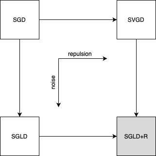
Figure 1 provides a diagram of our contributed scheme. Starting with SGD, one can add a carefully crafted noise term to arrive at the simplest SG-MCMC sampler, SGLD. Then, one can add repulsion between particles to speed-up the mixing time, leading to SGLD+R, our main contribution (Section 3).
After an overview of posterior approximation methods in Section 2, we propose our framework in Section 3. Section 4 discusses relevant experiments showcasing the benefits of our proposal. Finally, Section 5 sums up our contributions and highlight several open problems.
2 BACKGROUND AND RELATED WORK
Consider a probabilistic model and a prior distribution where denotes an observation and an unobserved dimensional latent variable or parameter, depending on the context. We are interested in performing inference regarding the unobserved variable , by approximating its posterior distribution:
Except for reduced classes of distributions like conjugate priors, Raiffa and Schlaifer (1961), the previous integral is analytically intractable; no general explicit expressions of the posterior are available. Thus, several techniques have been proposed to perform approximate posterior inference.
2.1 Inference as sampling
Hamiltonian Monte Carlo (HMC, Neal (2011)) is an effective sampling method for models whose probability is point-wise computable and differentiable. HMC requires the exact simulation of a certain dynamical system which can be cumbersome in high-dimensional or large data settings. When this is an issue, Welling and Teh (2011) proposed a formulation of a continuous-time Markov process that converges to a target distribution . It is based on the Euler-Maruyama discretization of Langevin dynamics:
| (1) |
where is the step size. The previous iteration uses the gradient evaluated at one data point , but we can use the full dataset or mini-batches. Several extensions of the original Langevin sampler have been proposed to increase mixing speed, see for instance Li et al. (2016a, b, 2019).
Ma et al. (2015) proposed a general formulation of a continuous-time Markov process that converges to a target distribution . It is based on the Euler-Maruyama discretization of the generalized Langevin dynamics:
| (2) | ||||
with being a diffusion matrix; , a curl matrix and is a correction term which amends the bias.
To obtain a valid SG-MCMC algorithm, we simply have to choose the dimensionality of (e.g., if we augment the space with auxiliary variables as in HMC), and the matrices and . For instance, the popular Stochastic Gradient Langevin Dynamics (SGLD) algorithm, the first SG-MCMC scheme in Welling and Teh (2011) in (1), is obtained when and . In addition, the Hamiltonian variant can be recovered if we augment the state space with a dimensional momentum term , leading to an augmented latent space . Then, we set and .
2.2 Inference as optimization
Variational inference, Kucukelbir et al. (2017), tackles the problem of approximating the posterior with a tractable parameterized distribution . The goal is to find parameters so that the variational distribution (also referred to as the variational guide or variational approximation) is as close as possible to the actual posterior. Closeness is typically measured through Kullback-Leibler divergence , which is reformulated into the evidence lower bound (ELBO), given by
| (3) |
To allow for greater flexibility, typically a deep non-linear model conditioned on observation defines the mean and covariance matrix of a Gaussian distribution . Inference is then performed using a gradient-based maximization routine, leading to variational parameter updates
where is the learning rate. Stochastic gradient descent (SGD), Hoffman et al. (2013), or some variant of it, such as Adam, Kingma and Ba (2014), are used as optimization algorithms.
On the other hand, SVGD, Liu and Wang (2016), frames posterior sampling as an optimization process, in which a set of particles is evolved iteratively via a velocity field , where is a smooth function characterizing the perturbation of the latent space. Assume that is the particle distribution at iteration and the distribution after update (). Then, the optimal choice of the velocity field can be framed through the optimization problem , in which is chosen to maximize the decreasing rate on the Kullback-Leibler (KL) divergence between the particle distribution and the target, and is some proper function space. When is a reproducing kernel Hilbert space (RKHS), Liu and Wang (2016) showed that the optimal velocity field leads to
| (4) | ||||
where the RBF kernel is typically adopted. Observe that in 4 the gradient term acts as a repulsive force that prevents particles from collapsing.
2.3 The Fokker-Planck equation
Consider a SDE of the form . The distribution of a population of particles evolving according to the previous SDE from some initial distribution is governed by the Fokker-Planck partial differential equation (PDE), Risken (1989),
Deriving the Fokker-Planck equation from the SDE of a potential SG-MCMC sampler is of great interest since we can check whether the target distribution is a stationary solution of the previous PDE (and thus, the sampler is consistent); and to compare if two a priori different SG-MCMC samplers result in the same trajectories.
2.4 Related work
There has been recent interest in developing new dynamics for SG-MCMC samplers with the aim of exploring the target distribution more efficiently. Chen et al. (2014) proposed a stochastic gradient version of HMC, and Ding et al. (2014) did the same leveraging for the Nosé-Hoover thermostat dynamics. Chen et al. (2016) leverages ideas from stochastic gradient optimization by proposing the analogue sampler to the Adam optimizer. A relativistic variant of Hamiltonian dynamics was introduced by Abbati et al. (2018). Two of the most recent derivations of SG-MCMC samplers are Zhang et al. (2019), in which the authors propose a policy controlling the learning rate which serves as a better preconditioning; and Gong et al. (2019), in which a meta-learning approach is proposed to learn an efficient SG-MCMC transition kernel.
While the previous works propose new kernels which can empirically work well, they focus on the case of a single chain. We instead consider the case of several chains in parallel, and the bulk of our contribution focuses on how to develop transition kernels which can exploit interactions between chains. Thus, our framework can be seen as an orthogonal development to the previous listed approaches, and could be combined with them.
On the theoretical side, Chen et al. (2018) study another connection between MCMC and deterministic flows, in particular they explore the correspondence between Langevin dynamics and Wasserstein gradient flows. We instead formulate the dynamics of SVGD as a particular kind of MCMC dynamics, which enables us to use the Fokker-Planck equation to show in an straightforward manner how our samplers are valid. Liu (2017) started to consider similitudes between SG-MCMC and SVGD, though in this work we propose the first hybrid scheme between both methods.
3 THE PROPOSED FRAMEWORK
We use the framework from Ma et al. (2015) in an augmented state space to obtain a valid posterior sampler that runs multiple () Markov chains with interactions. This version of SG-MCMC is given by the equation
| (5) |
with . Now, is an -dimensional vector defined by the concatenation of particles; so that 111Though to allow multiplication by , we reshape it as to better illustrate how it is defined.; is an expansion of the diffusion matrix , accounting for the distance between particles; is the curl matrix, which is skew-symmetric and might be used if a Hamiltonian variant is adopted; and is the correction term from the framework of Ma et al. (2015). Note that , and can depend on the state (an example will be given below), but we do not make it explicit to simplify notation.
In matrix form, the update rule (4) for SVGD can be expressed as
| (6) |
where so that , and . Casting the later matrix as a tensor and the former one as a tensor by broadcasting along the second and fourth axes, we may associate with the SG-MCMC’s diffusion matrix over a dimensional space.
The big matrix in Eq. (5) is defined as a permuted block-diagonal matrix consisting of repeated kernel matrices :
with being the permutation matrix
The permutation matrix rearranges the block-diagonal kernel matrix to match with the dimension ordering of the state space . With this convention, is equivalent to , only differing in the shape of the resulting matrix. This allows us to frame SVGD plus the noise term as a valid scheme within the SG-MCMC framework of Ma et al. (2015), using the -dimensional augmented state space.
From this perspective, Eq. (6) can be seen as a special case of Eq. (5) with curl matrix and no noise term. We refer to this perturbed variant of SVGD as Parallel SGLD plus repulsion (SGLD+R):
| (7) |
Since is a definite positive matrix (constructed from the RBF kernel), we may use the key result from Ma et al. (2015) (Theorem 1) to derive the following:
Proposition 1.
SGLD+R (or its general form, Eq. (5)) has as stationary distribution, and the proposed discretizations are asymptotically exact as .
Having shown that SVGD plus a noise term can be framed as an SG-MCMC method, we may now explore the design spaces of the and matrices.
Algorithm 1 shows how to set the sampler up. The step sizes decrease to using the Robbins-Monro conditions, Robbins and Monro (1951), given by . However, in practical situations we can consider a small and constant step size, see Section 4.
| (8) | ||||
Complexity.
Finally, our proposed method is amenable to sub-sampling, since the mini-batch setting from SG-MCMC can be adopted: the main computational bottleneck lies in the evaluation of the gradient , which can be troublesome in a big data setting such as when . We may then approximate the true gradient with an unbiased estimator taken along a minibatch of datapoints in the usual way:
As with the original SVGD algorithm, the complexity of the update rule (6) is , with being the number of particles, since we need to evaluate kernels of signature . Using current state-of-the-art automatic differentiation frameworks, such as jax, Bradbury et al. (2018), we can straightforwardly compile kernels using just-in-time compilation, Frostig et al. (2018), at the cost of a negligible overhead compared to parallel SGLD for moderate values of particles.
If many more particles are to be used, one could approximate the expectation in Eq. (6) using subsampling at each iteration, as proposed by the authors of SVGD, or by using more sophisticated approaches from the molecular dynamics literature, such as the Barnes-Hutt algorithm, Barnes and Hut (1986), to arrive at an efficient computational burden at a negligible approximation error. We leave this approximation for further work.
3.1 Relationship with SVGD
In this Section we study in detail the behaviour of SVGD and SGLD+R. To do so, we will derive the Fokker-Planck equation for the SGLD+R sampler first.
Proposition 2.
The distribution of a population of particles evolving according to SGLD+R is governed by
The target distribution is a stationary solution of the previous PDE.
Proof.
The first part is a straightforward application of the Fokker-Planck equation from Section 2.3. For the last part, we need to show that
To see so, we will expand each term in the rhs:
The other term expands to
Taking into account that by the definition of the correction term, , the previous expansions are equal so they cancel each other in the rhs of the PDE. ∎
This last result is an alternative proof of our Preposition 1, without having to resort to the framework of Ma et al. (2015) as was the case there. It is of independent interest for us here, since we can establish a complementary result for the case of SVGD as follows.
Proposition 3.
The distribution of a population of particles evolving according to SVGD is governed by
The target distribution is not a stationary solution of the previous PDE in general.
Proof.
As before, the first part is a straightforward application of the Fokker-Planck equation from Section 2.3. For the last part, note that the difference with Proposition 2 is that the term is absent now in the PDE, which prevents from being a stationary solution in general. ∎
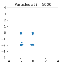
The term encourages the entropy in the distribution . By ignoring it, the SVGD flow achieves stationary solutions that underestimate the variance of the target distribution. On the other hand, SGLD+R, performs a correction, leading to the correct target distribution. In the next example we highlight this fact in a relatively simple setting.
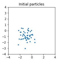
Example.
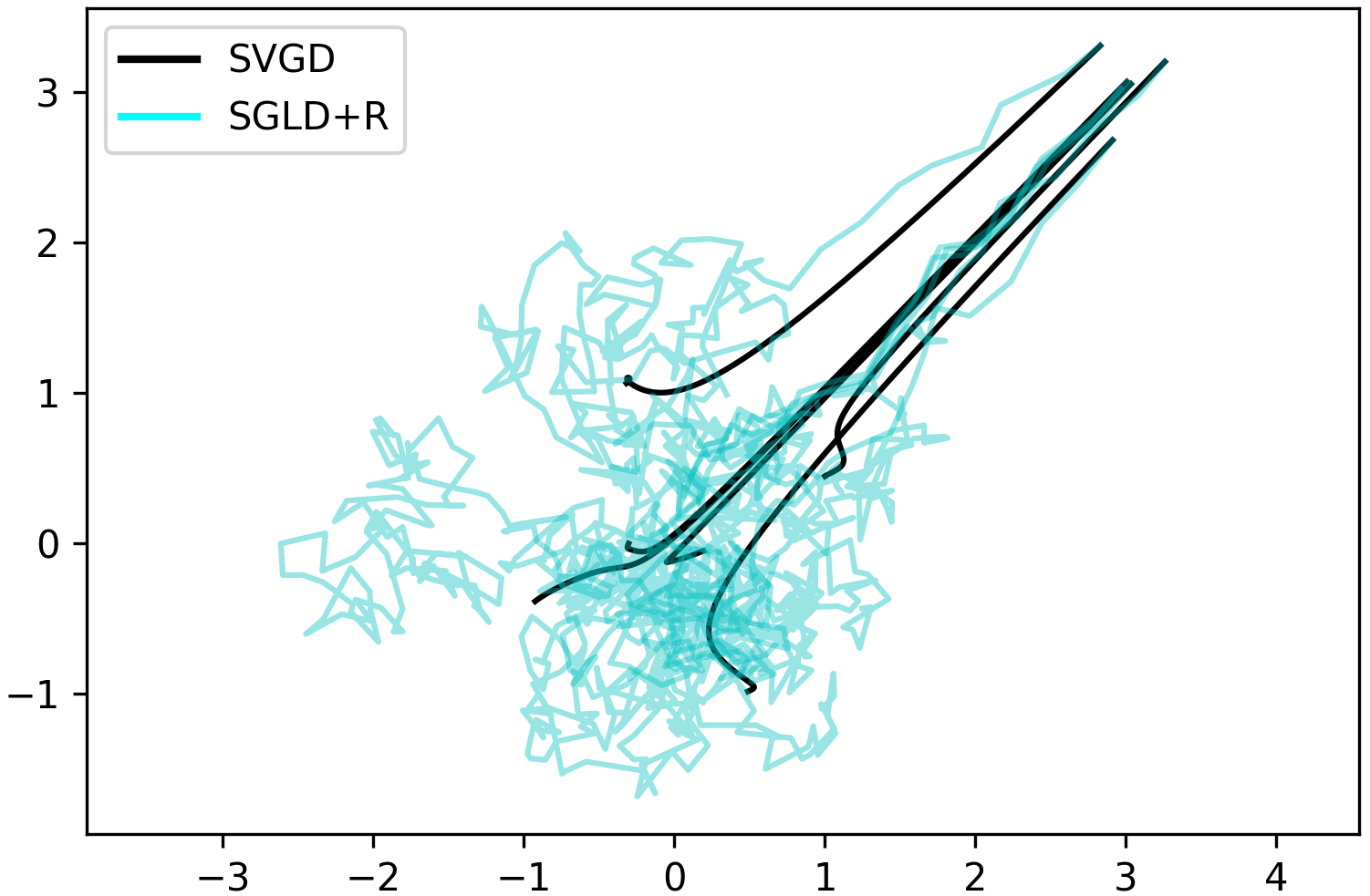
Consider a standard bi-dimensional Gaussian target, . The initial distribution of particles is . We let both samplers run for iterations using particles, and we plot their trajectories in Figure 2. Note how SGLD+R, since it is a valid sampler, explores a greater region of the target distribution, in comparison with SVGD, which underestimates the extension of the actual target. This phenomenon was predicted by Propositions 2 and 3. We also attach a Table, in which we report estimates of the target mean, , and marginal standard deviations, and , respectively. Notice how SGLD+R estimates are closer to the ground truth values for the standard Gaussian target of this example.
| Estimates | SVGD | SGLD+R | Target |
|---|---|---|---|
| 0.08 | 0.00 | ||
| 0.90 | 1.00 | ||
| 0.87 | 1.00 |
[table]A table beside a figure
4 EXPERIMENTS
This Section describes the experiments developed to empirically test the proposed scheme. After the example from Section 3.1, which compares SVGD and SGLD+R, we focus on confronting SGLD+R with the non-repulsive variant. First, we deal with two synthetic distributions, which offer a moderate account of complexity in the form of multimodality. In our second group of experiments, the focus is on a more challenging setting, testing a deep Bayesian model over several benchmark real data sets.
Code for the different samplers is open sourced at https://github.com/anon3232/sgmcmc-force. We rely on the library jax, Bradbury et al. (2018), as the main package, since it provides convenient automatic differentiation features with just-in-time compilation which is extremely useful in our case for an efficient implementation of the SG-MCMC transition kernels.
4.1 Synthetic distributions
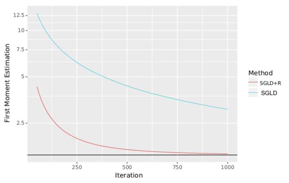
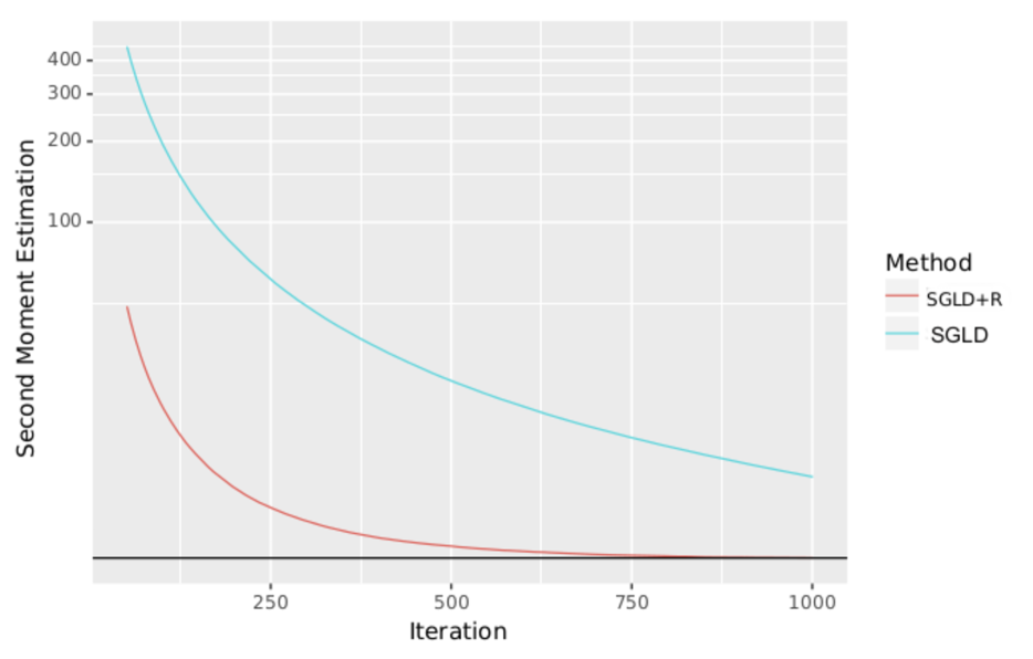
The goal of this experiment is to see how well the samples generated by our framework approximate some quantities of interest, which can be analytically computed since the distributions are known. We thus test our proposed scheme with the following distributions.
-
•
Mixture of Exponentials (MoE). Two exponential distributions with different scale parameters and mixture proportions . The pdf is
The exact value of the first and second moments can be computed using the change of variables formula
with . Since , to use the proposed scheme, we reparameterize using the function. The pdf of the transformation can be computed using
-
•
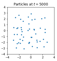
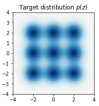
Mixture of 2D Gaussians (MoG). A grid of equally distributed isotropic 2D Gaussians, see Figure 5(d) for the density plot. We set and place the nine Gaussians centered at the following points:
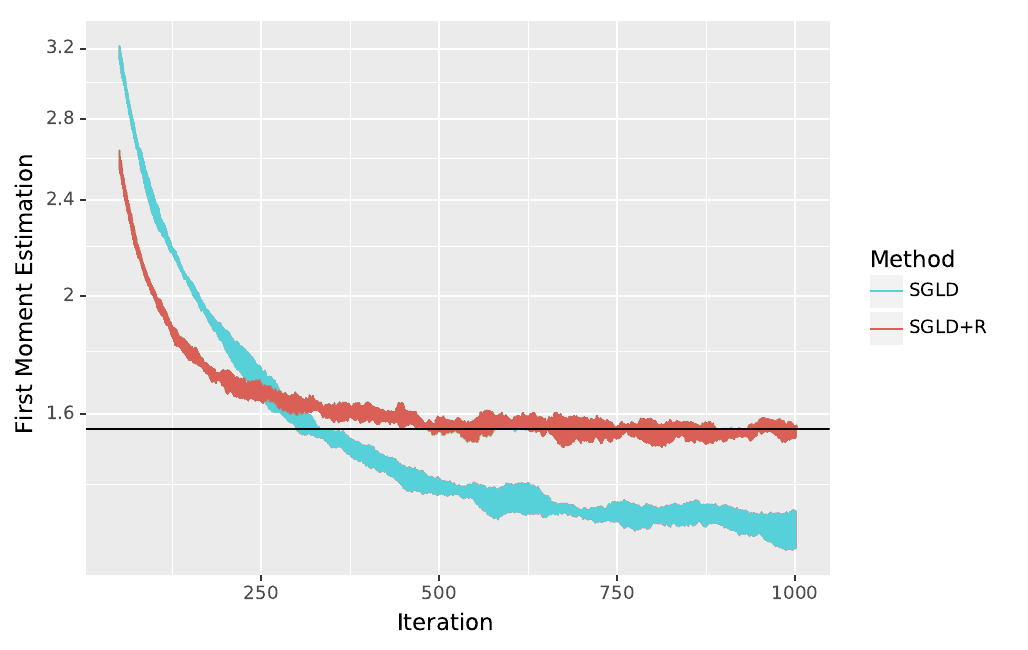
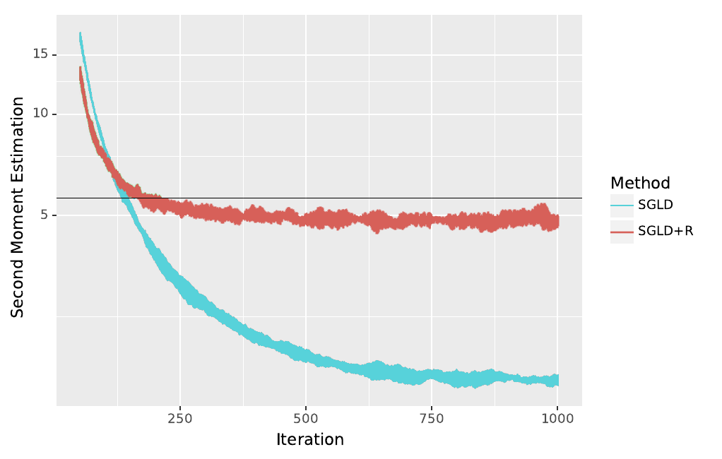
We compare two sampling methods, SGLD with parallel chains, and our proposed scheme, SGLD+R. Note that the main difference between these two sampling algorithms is that for the former whereas the latter accounts for repulsion between particles. Table 1 reports the effective sampling size metrics, Kass et al. (1998), for each method using particles. Note that while ESS/s are similar, the repulsive forces in SGLD+R make for a more efficient exploration, resulting in much lower estimation errors. Figures 3 and 5 confirm this fact. In addition, even when increasing the number of particles , SGLD+R achieves lower errors than SGLD (see Fig. 4).
For the computation of the error of in Tables 1 and 2, we sample for 500 iterations after discarding the first 500 iterations as burn-in, and we collect samples every 10 iterations to reduce correlation between samples. For the MoE case we used 10 particles whereas for the MoG task we used 20 particles given the bigger number of modes.
| ESS | ESS/s | |||
|---|---|---|---|---|
| Distribution | SGLD | SGLD+R | SGLD | SGLD+R |
| MoE | ||||
| MoG | ||||
| Error of | ||
|---|---|---|
| Distribution | SGLD | SGLD+R |
| MoE | ||
| MoG | ||
4.2 Bayesian Neural Network
We test the proposed scheme in a suite of regression tasks using a feed-forward neural network with one hidden layer with 50 units and ReLU activations. The goal of this experiment is to check that the proposed samplers scale well to real-data settings and complex models such as Bayesian neural networks. The datasets are taken from the UCI repository, Lichman (2013). We use minibatches of size 100. As before, we compare SGLD and SGLD+R, reporting the average root mean squared error and log-likelihood over a test set in Table 3 and Table 4. We observe that SGLD+R typically outperforms SGLD. During the experiments, we noted that in order to reduce computation time, during the last half of training we could disable the repulsion between particles without incurring in performance cost.
The learning rate was chosen from a grid validated on another fold. The number of iterations was set to 2000 in every experiment. As before, to make predictions we collect samples every 10 iterations after a burn-in period. 20 particles were used for each of the tested datasets.
| Avg. Test LL | ||
|---|---|---|
| Dataset | SGLD | SGLD+R |
| Boston | ||
| Kin8nm | ||
| Naval | ||
| Protein | ||
| Wine | ||
| Yacht | ||
| Avg. Test RMSE | ||
|---|---|---|
| Dataset | SGLD | SGLD+R |
| Boston | ||
| Kin8nm | ||
| Naval | ||
| Protein | ||
| Wine | ||
| Yacht | ||
5 CONCLUSIONS AND FURTHER WORK
This paper shows how to generate new SG-MCMC methods, such as our main contribution, SGLD+R, consisting of multiple chains plus repulsion between the particles. Instead of the naive parallelization, in which a particle from a chain is agnostic to the others, we showed how it is possible to adapt another method from the literature, SVGD, to account for a better exploration of the space, avoiding collapse between particles. We also studied the behaviour of both SVGD and SGLD+R using the Fokker-Planck equation and noting that whereas SVGD cannot be used as a valid SG-MCMC sampler, the introduction of a noise term as in SGLD+R indeed enables convergence to the actual posterior in the limit. Our experiments show that the proposed ideas improve efficiency when dealing with large scale inference and prediction problems in presence of many parameters and large data sets.
Several avenues are open for further work. Here we discuss only several promising ones. First, with a very large particle regime () there is room to use approximating algorithms such as Barnes-Hutt to keep the computational cost tractable. Secondly, we used the RBF kernel in all our experiments, but a natural issue to address would be to define a parameterized kernel and learn the parameters on the go to optimize the ESS/s rate, using meta-learning approaches such as the one proposed in Gallego and Insua (2019) for the SGLD case.
Acknowledgments VG acknowledges support from grant FPU16-05034. DRI is grateful to the MINECO MTM2017-86875-C3-1-R project and the AXA-ICMAT Chair in Adversarial Risk Analysis. All authors acknowledge support from the Severo Ochoa Excellence Programme SEV-2015-0554 and US National Science Foundation through grant DMS-1638521.
References
- Abbati et al. [2018] G. Abbati, A. Tosi, M. Osborne, and S. Flaxman. Adageo: Adaptive geometric learning for optimization and sampling. In International Conference on Artificial Intelligence and Statistics, pages 226–234, 2018.
- Barnes and Hut [1986] J. Barnes and P. Hut. A hierarchical o (n log n) force-calculation algorithm. Nature, 324(6096):446, 1986.
- Bishop [2006] C. M. Bishop. Pattern recognition and machine learning. Springer, 2006.
- Blei et al. [2017] D. M. Blei, A. Kucukelbir, and J. D. McAuliffe. Variational inference: A review for statisticians. Journal of the American Statistical Association, 112(518):859–877, 2017.
- Bradbury et al. [2018] J. Bradbury, R. Frostig, P. Hawkins, M. J. Johnson, C. Leary, D. Maclaurin, and S. Wanderman-Milne. JAX: composable transformations of Python+NumPy programs, 2018. URL http://github.com/google/jax.
- Carbonetto and Stephens [2012] P. Carbonetto and M. Stephens. Scalable variational inference for bayesian variable selection in regression, and its accuracy in genetic association studies. Bayesian Anal., 7(1):73–108, 03 2012. doi: 10.1214/12-BA703. URL https://doi.org/10.1214/12-BA703.
- Chen et al. [2016] C. Chen, D. Carlson, Z. Gan, C. Li, and L. Carin. Bridging the gap between stochastic gradient mcmc and stochastic optimization. In Artificial Intelligence and Statistics, pages 1051–1060, 2016.
- Chen et al. [2018] C. Chen, R. Zhang, W. Wang, B. Li, and L. Chen. A unified particle-optimization framework for scalable bayesian sampling. arXiv preprint arXiv:1805.11659, 2018.
- Chen et al. [2014] T. Chen, E. Fox, and C. Guestrin. Stochastic gradient hamiltonian monte carlo. In International Conference on Machine Learning, pages 1683–1691, 2014.
- Ding et al. [2014] N. Ding, Y. Fang, R. Babbush, C. Chen, R. D. Skeel, and H. Neven. Bayesian sampling using stochastic gradient thermostats. In Advances in Neural Information Processing Systems, pages 3203–3211, 2014.
- Frostig et al. [2018] R. Frostig, M. J. Johnson, and C. Leary. Compiling machine learning programs via high-level tracing. 2018.
- Gallego and Insua [2019] V. Gallego and D. R. Insua. Variationally inferred sampling through a refined bound. In Advances in Approximate Bayesian Inference (AABI), 2019.
- Gelman et al. [2013] A. Gelman, J. B. Carlin, H. S. Stern, D. B. Dunson, A. Vehtari, and D. B. Rubin. Bayesian data analysis. Chapman and Hall/CRC, 2013.
- Gong et al. [2019] W. Gong, Y. Li, and J. Hernández-Lobato. Meta-learning for stochastic gradient mcmc. In 7th International Conference on Learning Representations, ICLR 2019, 2019.
- Hoffman et al. [2013] M. D. Hoffman, D. M. Blei, C. Wang, and J. Paisley. Stochastic variational inference. The Journal of Machine Learning Research, 14(1):1303–1347, 2013.
- Kass et al. [1998] R. E. Kass, B. P. Carlin, A. Gelman, and R. M. Neal. Markov chain monte carlo in practice: a roundtable discussion. The American Statistician, 52(2):93–100, 1998.
- Kingma and Ba [2014] D. P. Kingma and J. Ba. Adam: A method for stochastic optimization. arXiv preprint arXiv:1412.6980, 2014.
- Kucukelbir et al. [2017] A. Kucukelbir, D. Tran, R. Ranganath, A. Gelman, and D. M. Blei. Automatic differentiation variational inference. The Journal of Machine Learning Research, 18(1):430–474, 2017.
- Li et al. [2016a] C. Li, C. Chen, D. Carlson, and L. Carin. Preconditioned stochastic gradient langevin dynamics for deep neural networks. In Thirtieth AAAI Conference on Artificial Intelligence, 2016a.
- Li et al. [2016b] C. Li, C. Chen, K. Fan, and L. Carin. High-order stochastic gradient thermostats for bayesian learning of deep models. In Thirtieth AAAI Conference on Artificial Intelligence, 2016b.
- Li et al. [2019] C. Li, C. Chen, Y. Pu, R. Henao, and L. Carin. Communication-efficient stochastic gradient mcmc for neural networks. 2019.
- Lichman [2013] M. Lichman. UCI Machine Learning Repository. http://archive.ics.uci.edu/ml, 2013.
- Liu [2017] Q. Liu. Stein variational gradient descent as gradient flow. In Advances in Neural Information Processing Systems, pages 3115–3123, 2017.
- Liu and Wang [2016] Q. Liu and D. Wang. Stein variational gradient descent: A general purpose bayesian inference algorithm. In Avances In Neural Information Processing Systems, pages 2378–2386, 2016.
- Ma et al. [2015] Y.-A. Ma, T. Chen, and E. Fox. A complete recipe for stochastic gradient mcmc. In C. Cortes, N. D. Lawrence, D. D. Lee, M. Sugiyama, and R. Garnett, editors, Advances in Neural Information Processing Systems 28, pages 2917–2925. Curran Associates, Inc., 2015.
- Neal [2011] R. M. Neal. Mcmc using hamiltonian dynamics. In Handbook of Markov Chain Monte Carlo, pages 139–188. Chapman and Hall/CRC, 2011.
- Raiffa and Schlaifer [1961] H. Raiffa and R. Schlaifer. Applied statistical decision theory. Studies in managerial economics. Division of Research, Graduate School of Business Adminitration, Harvard University, 1961. ISBN 9780875840178. URL https://books.google.es/books?id=wPBLAAAAMAAJ.
- Riquelme et al. [2018] C. Riquelme, M. Johnson, and M. Hoffman. Failure modes of variational inference for decision making. 2018. URL http://reinforcement-learning.ml/papers/pgmrl2018_riquelme.pdf.
- Risken [1989] H. Risken. The Fokker-Planck Equation: Methods of Solutions and Applications, 2nd ed. Springer Verlag, Berlin, Heidelberg, 1989.
- Robbins and Monro [1951] H. Robbins and S. Monro. A stochastic approximation method. The annals of mathematical statistics, pages 400–407, 1951.
- Welling and Teh [2011] M. Welling and Y. W. Teh. Bayesian learning via stochastic gradient langevin dynamics. In Proceedings of the 28th International Conference on Machine Learning (ICML-11), pages 681–688, 2011.
- Yao et al. [2018] Y. Yao, A. Vehtari, D. Simpson, and A. Gelman. Yes, but did it work?: Evaluating variational inference. In J. Dy and A. Krause, editors, Proceedings of the 35th International Conference on Machine Learning, volume 80 of Proceedings of Machine Learning Research, pages 5581–5590, Stockholmsmässan, Stockholm Sweden, 10–15 Jul 2018. PMLR. URL http://proceedings.mlr.press/v80/yao18a.html.
- Zhang et al. [2018] C. Zhang, B. Shahbaba, and H. Zhao. Variational hamiltonian monte carlo via score matching. Bayesian Anal., 13(2):485–506, 06 2018. doi: 10.1214/17-BA1060. URL https://doi.org/10.1214/17-BA1060.
- Zhang et al. [2019] R. Zhang, C. Li, J. Zhang, C. Chen, and A. G. Wilson. Cyclical stochastic gradient mcmc for bayesian deep learning. arXiv preprint arXiv:1902.03932, 2019.