A Basic Introduction to the Physics of Solar Neutrinos

Abstract

A comprehensive introduction to the theory of the solar neutrino problem is given that is aimed at instructors who are not experts in quantum field theory but would like to incorporate these ideas into instruction of advanced undergraduate or beginning graduate students in courses like astrophysics or quantum mechanics; it is also aimed at the inquisitive student who would like to learn this topic on their own. The presentation assumes as theoretical preparation only that the reader is familiar with the basics of quantum mechanics in Dirac notation and elementary differential equations and matrices.

I Introduction

The resolution of the solar neutrino problem in terms of neutrino flavor oscillations has had an enormous impact on both astrophysics and elementary particle physics. On the one hand, it has demonstrated that the Standard Solar Model (SSM) works remarkably well, and has suggested profitable new directions in a number of astrophysics subfields, while on the other hand it has demonstrated conclusively that there is physics beyond the Standard Model (SM) of elementary particle physics and has suggested possible clues for what that new physics could be. It is fitting then that the importance of these ideas was recognized in both the 2002 and 2015 Nobel Prizes in Physics. Presumably for these and related reasons, we have found that solar neutrino oscillations attract more enthusiastic responses from students in advanced undergraduate and graduate courses on stellar structure and stellar evolution than any other topic.

Neutrino oscillations in vacuum and in matter are described extensively in the journal literature and in textbooks but most of those discussions are either conceptual overviews, walt2004 ; hax00 ; hax04 necessarily omitting a systematic mathematical formulation of solar neutrino theory, or treat solar neutrino theory extensively but are written assuming that the reader has a substantial background in quantum field theory of the weak interactions. kuo1989 ; smir2003 ; blen2013 Most advanced undergraduate and beginning graduate students interested in this problem, and instructors who are not experts but wish to understand and incorporate this topic into their courses, will find neither to be ideal sources by themselves. The first introduces the concepts well but omits much of the deep mathematical ‘why’ and ‘how’ of these beautiful ideas; the second formulates the theory more systematically but typically requires a substantial remedial effort for the intelligent non-expert to come up to the required speed, often omitting important steps in derivations that are (relatively) obvious to the cognoscenti, but perhaps not to others.

This paper attempts to provide a systematic introduction to solar neutrino oscillations and the resolution of the solar neutrino problem at a level that will satisfy non-specialist instructor and student alike within an accessible mathematical framework. It assumes only that the reader is familiar initially with mathematics and basic quantum mechanics at a level characteristic of an advanced undergraduate physics major. No particular background in solar astrophysics, elementary particle physics, or relativistic quantum field theory is assumed, as the required concepts are introduced as part of the presentation.

II Solar Neutrinos and the Standard Model

We begin with a concise overview of solar neutrinos and of the Standard Model of elementary particles, and of why neutrino observations led to a “solar neutrino problem” implying that either our understanding of the Sun, or our understanding of the neutrino, or perhaps both, required fixing. The approach will be decidedly pragmatic, describing only aspects of these two fields that are directly relevant to the task at hand.

II.1 Neutrinos in the Standard Solar Model

The Sun is powered by nuclear reactions taking place in its core that convert hydrogen into helium and release energy in the process. Two different mechanisms can accomplish this: (1) the PP chains, and (2) the CNO cycle. At its present core temperature almost 99% of the Sun’s energy is provided by the PP chains, so they will be our focus. The details of these nuclear reactions are well documented and will not be of direct concern here, except to note that some of these reactions are weak interactions that produce neutrinos and that these can be detected on Earth. This is of large importance in astrophysics because the neutrinos are produced in the core and leave the Sun at essentially the speed of light, with little probability to react with the solar matter. Thus their detection on Earth provides a snapshot of conditions in the solar core approximately 8.5 minutes prior to detection, and a stringent test of solar models specifically and, by implication, of more general models for stellar structure and stellar evolution.

For our specific purposes all that is relevant concerning these solar neutrino-producing reactions are the flavor (neutrino type) and spectrum of the neutrinos that are produced, and the electron density distribution in the solar interior. These may be obtained from the semi-phenomenological Standard Solar Model, which combines the theory of stellar structure and evolution with the values of key parameters inferred from measurements or theory to provide a comprehensive and predictive model for the structure and evolution of the Sun. bah89 The spectrum of solar neutrinos predicted by the SSM is displayed in Fig. 1,

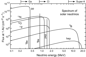
Figure 1: The SSM neutrino spectrum, with fluxes scaled to the distance of Earth from the Sun. bah01 Labels refer to specific reactions in the PP chains and CNO cycle. The sensitive regions for various experiments are indicated above the graph, with Ga denoting the GALLEX and SAGE gallium detectors, Cl denoting the Homestake (Davis) chlorine detector, and Super K denoting the Super Kamiokande water Cherenkov detector (see Table 1).

and the electron number density as a function of radius from the SSM is displayed in Fig. 2.

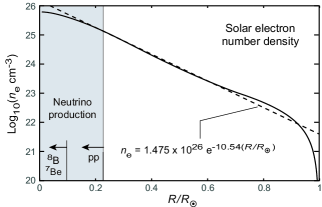
Figure 2: Electron number density as a function of fractional solar radius from the Standard Solar Model. bah01 The dashed line is an exponential approximation that will be employed in discussing the MSW effect. Regions of primary neutrino production in the PP chains are indicated, using labels from Fig. 1.

When solar neutrinos are detected on Earth by chemistry-based or normal-water Cherenkov detectors, the flux is found to be systematically less than that predicted by the SSM (see Fig. 1), in an amount that depends on the energy of the neutrinos; Table 1 illustrates.

Table 1: Solar neutrino fluxes from various experiments compared with a Standard Solar Model (SSM) calculated in Ref. bah95, . All fluxes are in solar neutrino units (SNU), except the result from Super Kamiokande. (1 SNU is the neutrino flux that would produce $10^{-36}$ interactions per target atom per second.) Experimental uncertainties include systematic and statistical contributions.

Experiment	Observed flux	SSM	Observed/SSM
Homestake	$2.54\pm 0.14\pm 0.14\mbox{\ SNU}$	$9.3^{\ +1.2}_{\ -1.4}$	$0.273\pm 0.021$
SAGE	$72^{\ +12\ +5}_{\ -10\ -7}\mbox{\ SNU}$	$137^{\ +8}_{\ -7}$	$0.526\pm 0.089$
GALLEX	$69.7\pm 6.7^{\ +3.9}_{\ -4.5}\mbox{\ SNU}$	$137^{\ +8}_{\ -7}$	$0.509\pm 0.089$
Super Kamiokande	$2.51^{\ +0.14}_{\ -0.13}\ (10^{6}\mbox{\ cm${}^{-2}$s${}^{-1}$})$	$6.62^{\ +0.93}_{\ -1.12}$	$0.379\pm 0.034$

Typically for the highest neutrino energies the observed flux is around $30\%$ of that expected while for the lowest energies about $50\%$ the expected number are seen. This is the famous solar neutrino problem. The reproducibility in independent experiments of the measured flux suppression from that expected indicates that the issue is real, and implies some combination of (1) the Standard Solar Model fails to describe properly the conditions in the Sun’s core (we don’t understand the Sun), or (2) the properties of neutrinos differ from that assumed in the prediction of Fig. 1 (we don’t understand the neutrino). To investigate these possibilities, let us now consider the description of neutrinos and the weak interactions in the Standard Model of elementary particle physics that is implicit in the prediction of Fig. 1.

II.2 The Standard Model and Weak Interactions

The Standard Model of elementary particle physics is the most comprehensive and well-tested theory yet conceived in theoretical physics, and it accounts for an extremely broad range of phenomena. However, our purposes are specific and require only four basic ingredients and one speculation from the SM: (1) the generational structure of its elementary fermions (matter fields) and associated lepton-number conservation laws (see §II.2.1), (2) the corresponding implication that neutrinos must be identically massless and that only left-handed neutrinos and right-handed antineutrinos enter the weak interactions (which builds the maximal breaking of parity symmetry into the weak interactions by fiat), (3) the empirical observation that in the quark sector the weak eigenstates are not congruent with the mass eigenstates, implying flavor mixing (see §II.2.2 and §II.2.3), (4) the long-standing speculation bono2005 that flavor oscillations might occur in the neutrino sector also (which would imply finite masses for neutrinos and thus a violation of the minimal Standard Model) (see §III), and (5) that the weak interactions can occur through charged currents mediated by the $W^{\pm}$ bosons and neutral currents mediated by the $Z^{0}$ boson (see §III.1).

II.2.1 Generational Structure

The fermions of the Standard Model are grouped into three families or generations, as displayed in Fig. 3.

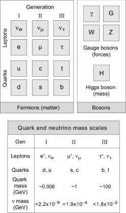
Figure 3: Particles of the Standard Model and characteristic mass scales in the quark and neutrino sectors for each generation. PDG

In the SM, interactions across family lines are forbidden. For the leptons this is implemented formally by assigning a lepton family number to each particle and requiring that it be conserved by interactions. The term flavor is used to distinguish the quarks and leptons of one generation from another. Thus, $(\nu_{\mbox{\scriptsize e}}$, $\nu_{\mu},\nu_{\tau})$ are different flavors of neutrinos, and (u, d, s, …) are different flavors of quarks.

Also displayed in Fig. 3 are characteristic mass scales for quarks and neutrinos within each generation. The neutrino masses are upper limits, since no neutrino mass has yet been measured directly. They are seen to be tiny on a mass scale set by the quarks of a generation, which is a major unresolved issue. There is no known fundamental reason why the neutrino masses should be identically zero (as assumed phenomenologically in the SM), and if they are not identically zero, then why are they so small?

II.2.2 Flavor Mixing in the Quark Sector

The Standard Model is made richer and more complex by the experimental observation of flavor mixing in the quark sector. For quarks the mass eigenstates and the weak eigenstates are not equivalent, which means that the quark states that enter the weak interactions (flavor eigenstates) are generally linear combinations of the mass eigenstates (eigenstates of propagating quarks). For example, restricting to the first two generations, it is found that the d and s quarks enter the weak interactions in the “rotated” linear combinations $d_{\mbox{\scriptsize c}}$ and $s_{\mbox{\scriptsize c}}$ defined by the matrix equation

$$\begin{pmatrix}d_{\mbox{\scriptsize c}}\\ s_{\mbox{\scriptsize c}}\end{pmatrix}=\begin{pmatrix}\cos\theta_{\mbox{\scriptsize c}}&\sin\theta_{\mbox{\scriptsize c}}\\ -\sin\theta_{\mbox{\scriptsize c}}&\cos\theta_{\mbox{\scriptsize c}}\end{pmatrix}\begin{pmatrix}d\\ s\end{pmatrix}$$ (1)

where $d$ and $s$ are mass-eigenstate quark fields and the $2\times 2$ unitary matrix is parameterized by $\theta_{\mbox{\scriptsize c}}$, which is termed the mixing angle or the Cabibbo angle. Data require the mixing angle to be rather small: $\theta_{\mbox{\scriptsize c}}\sim 13^{\circ}$. In the more general case of three generations of quarks, weak eigenstates are described by a $3\times 3$ mixing matrix called the Cabibbo–Kobayashi–Maskawa or CKM matrix, which has three real mixing angles and one phase. There is little fundamental understanding of this quark flavor mixing but data clearly require it.

II.2.3 Flavor Mixing in the Leptonic Sector?

Observation of flavor mixing among quarks raises the question of whether similar mixing could occur among the neutrino flavors. This is irrelevant in the Standard Model because to be observable the neutrino flavors undergoing mixing must have different masses, which is impossible in the SM where all neutrinos necessarily are identically massless. The possibility of flavor oscillations among neutrinos is intriguing because it could have large implications both for astrophysics and for particle physics. First, the Sun produces electron neutrinos $\nu_{\mbox{\scriptsize e}}$ and the initial neutrino detection experiments that found the solar neutrino problem were sensitive essentially only to $\nu_{\mbox{\scriptsize e}}$. If solar neutrinos can undergo flavor oscillations, then some $\nu_{\mbox{\scriptsize e}}$ produced by the Sun could reach the Earth as muon neutrinos $\nu_{\mu}$ or tao neutrinos $\nu_{\tau}$ that would not be detected, thus possibly accounting for the solar neutrino deficit exhibited in Table 1. Second, observation of neutrino oscillations would imply that at least one neutrino flavor has a finite mass, indicating that there must be physics beyond the Standard Model. Thus motivated, let us develop a theory of flavor oscillations for neutrinos.

III Neutrino Vacuum Oscillations

There are three known neutrino (and three antineutrino) flavors, but phenomenology suggests that solar neutrinos are well understood in terms of a simple mixing model for two flavors that will be employed here. We address first the simplest case of flavor oscillations for neutrinos propagating in vacuum. Then the more difficult (and interesting) issue of how the coupling of neutrinos to matter alters flavor oscillations will be taken up. In much of this development the convention that is standard in particle physics of choosing natural units, where both $\hbar$ and the speed of light $c$ are set to one, will be employed. The Appendix illustrates the relationship between natural units and standard units.

III.1 Mixing for Two Neutrino Flavors

To be definite the two flavors will be assumed to correspond to the electron neutrino with wavefunction $\nu_{\mbox{\scriptsize e}}\equiv|\nu_{\mbox{\scriptsize e}}\rangle$ and the muon neutrino with wavefunction $\nu_{\mu}\equiv|\nu_{\mu}\rangle$, but the formalism could be applied to the mixing any two flavors. By analogy with Eq. (1) for quarks, the flavor eigenstates $\nu_{\mbox{\scriptsize e}}$ and $\nu_{\mu}$ are assumed to be related to the mass eigenstates $\nu_{1}\equiv|\nu_{1}\rangle$ and $\nu_{2}\equiv|\nu_{2}\rangle$ through the matrix transformation

$$\begin{pmatrix}\nu_{\mbox{\scriptsize e}}\\ \nu_{\mu}\end{pmatrix}=U(\theta)\begin{pmatrix}\nu_{1}\\ \nu_{2}\end{pmatrix}=\begin{pmatrix}\cos\theta&\sin\theta\\ -\sin\theta&\cos\theta\end{pmatrix}\begin{pmatrix}\nu_{1}\\ \nu_{2}\end{pmatrix},$$ (2)

where $\theta$ is a phenomenological vacuum mixing angle chosen to lie in the range $0-45^{\circ}$, and the matrix $U$ is parameterized by the single real angle $\theta$. The matrix $U$ is unitary (and orthogonal), so $UU^{\dagger}=U^{\dagger}U=1$, where $U^{\dagger}$ is the hermitian conjugate of $U$ (in a matrix representation, interchange rows and columns, and complex conjugate all elements). This may be used to invert Eq. (2) and express the mass eigenstates as a linear combination of the flavor eigenstates:

$$\begin{pmatrix}\nu_{1}\\ \nu_{2}\end{pmatrix}=U(\theta)^{\dagger}\begin{pmatrix}\nu_{\mbox{\scriptsize e}}\\ \nu_{\mu}\end{pmatrix}=\begin{pmatrix}\cos\theta&-\sin\theta\\ \sin\theta&\cos\theta\end{pmatrix}\begin{pmatrix}\nu_{\mbox{\scriptsize e}}\\ \nu_{\mu}\end{pmatrix}.$$ (3)

Assuming that the mass is non-zero for at least one neutrino flavor, the different mass eigenstates will have slightly different energies as neutrinos propagate. Thus, the probability of detecting a specific neutrino flavor will oscillate with time, or with distance traveled. From relativistic quantum field theory applied to left-handed neutrinos (see Section IV.2.1), the mass eigenstates evolve with time $t$ according to

$$|\nu_{i}(t)\rangle=e^{-iE_{i}t}|\nu_{i}(0)\rangle,$$ (4)

where the index $i$ labels mass eigenstates of energy $E_{i}$, so the time evolution of the $\nu_{\mbox{\scriptsize e}}$ state in Eq. (2) will be given by

$$|\nu(t)\rangle=\cos\theta e^{-iE_{1}t}|\nu_{1}(0)\rangle+\sin\theta e^{-iE_{2}t}|\nu_{2}(0)\rangle,$$ (5)

and from the transformation (3) this may be expressed as the mixed-flavor state

$$|\nu(t)\rangle =(\cos^{2}\theta e^{-iE_{1}t}+\sin^{2}\theta e^{-iE_{2}t})|\nu_{\mbox{\scriptsize e}}\rangle$$

$$\quad+\sin\theta\cos\theta(-e^{-iE_{1}t}+e^{-iE_{2}t})|\nu_{\mu}\rangle.$$ (6)

Taking the overlap of this expression with the flavor eigenstates $|\nu_{\mbox{\scriptsize e}}\rangle$ and $|\nu_{\mu}\rangle$, the probabilities that a neutrino initially in an electron neutrino flavor state will remain an electron neutrino, or instead be converted to a muon neutrino after a time $t$, are given respectively by

$$P(\nu_{\mbox{\scriptsize e}}{\,\scriptstyle\rightarrow}\,\nu_{\mbox{\scriptsize e}},\,t) =|\langle\nu_{\mbox{\scriptsize e}}|\nu(t)\rangle|^{2}$$

$$=1-\tfrac{1}{2}\sin^{2}(2\theta)[1-\cos(E_{2}-E_{1})t],$$ (7a)

$$P(\nu_{\mbox{\scriptsize e}}{\,\scriptstyle\rightarrow}\,\nu_{\mu},\,t) =|\langle\nu_{\mu}|\nu(t)\rangle|^{2}$$

$$=\tfrac{1}{2}\sin^{2}(2\theta)[1-\cos(E_{2}-E_{1})t],$$ (7b)

with the sum of the two probabilities necessarily equal to unity.

III.2 The Vacuum Oscillation Length

Equations (7) define the essence of vacuum neutrino oscillations in a 2-flavor model. However, it is normal to put these results into a more practical form through the following considerations. Neutrinos have at most a tiny mass $m_{i}$, so $E_{i}{\ \scriptstyle>>\ }m_{i}c^{2}$ and the relativistic energy expression may be approximated using a binomial expansion,

$$E_{i}=(p^{2}+m_{i}^{2})^{1/2}\simeq p+\frac{m_{i}^{2}}{2p}.$$ (8)

Thus, assuming that $E_{1}\sim E_{2}\equiv E$,

$$E_{2}-E_{1}\simeq\frac{\Delta m^{2}}{2E}\qquad\Delta m^{2}\equiv m_{2}^{2}-m_{1}^{2}.$$ (9)

The probability for flavor survival and flavor conversion as a function of distance traveled $r\sim ct$ may then be expressed as

$$P(\nu_{\mbox{\scriptsize e}}{\,\scriptstyle\rightarrow}\,\nu_{\mbox{\scriptsize e}},\,r)=1-\sin^{2}2\theta\sin^{2}\left(\displaystyle\frac{\pi r}{L}\right),$$ (10a)

$$P(\nu_{\mbox{\scriptsize e}}{\,\scriptstyle\rightarrow}\,\nu_{\mu},\,r)=\sin^{2}2\theta\sin^{2}\left(\displaystyle\frac{\pi r}{L}\right),$$ (10b)

where $\theta$ is the (vacuum) mixing angle and the (vacuum) oscillation length $L$, defined by

$$L\equiv\frac{4\pi E}{\Delta m^{2}}=\frac{4\pi E\hbar c}{\Delta m^{2}c^{4}},$$ (11)

is the distance required for one one complete flavor oscillation. [In Eq. (11) $L$ is expressed first in $\hbar=c=1$ units and then in normal “engineering units” with factors of $\hbar$ and $c$ restored; see further discussion in the Appendix.] Neutrino oscillations for a 2-flavor model using these formulas are illustrated in Fig. 4.

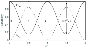
Figure 4: Neutrino vacuum oscillations in a 2-flavor model as a function of distance traveled $r\sim ct$, with $r$ in units of the vacuum oscillation length $L$. The probability as a function of $r$ to be an electron neutrino is denoted by $P_{\nu_{\mbox{\scriptsize e}}}$ and that to be a muon neutrino by $P_{\nu_{\mu}}$. The period of the oscillation is $L$ and its amplitude is $\sin^{2}2\theta$, where $\theta$ is the vacuum mixing angle. In this calculation $\theta=33.5^{\circ}$, the neutrino energy is $E=5\mbox{\ MeV}$, the difference in squared masses for the two flavors is $\Delta m^{2}c^{4}=7.5\times 10^{-5}\mbox{\ eV}^{2}$, and the corresponding oscillation length $L$ is $165.3\mbox{\ km}$.

III.3 Time-Averaged or Classical Probabilities

In observations the oscillation length may be smaller than the uncertainties in position for emission and detection of neutrinos. This will usually be the case for solar neutrinos, where oscillation lengths are typically several hundred kilometers but there are variation of thousands of kilometers in the distance traversed between production in the Sun and detection on Earth. If the oscillation length is less than the averaging introduced by the preceding considerations, the detectors will see a distance (or time) average of Eq. (10). Denoting the averaged probability by a bar gives

$$\begin{array}[]{c}\bar{P}(\nu_{\mbox{\scriptsize e}}{\,\scriptstyle\rightarrow\,}\nu_{\mbox{\scriptsize e}})=1-\tfrac{1}{2}\sin^{2}2\theta\quad\bar{P}(\nu_{\mbox{\scriptsize e}}{\,\scriptstyle\rightarrow\,}\nu_{\mu})=\tfrac{1}{2}\sin^{2}2\theta,\end{array}$$ (12)

for the probability (10) of detecting the two flavors distance-averaged over the oscillating factor. This may also be viewed as the classical probability, since the same formula results if the quantum interference resulting from squaring the sum of probability amplitudes is removed from the probability. For two flavors the instantaneous probability to remain a $\nu_{\mbox{\scriptsize e}}$ can approach zero if the mixing angle is large (see Fig. 4) but the average survival probability has a lower limit of $\frac{1}{2}$ for two flavors. The lower limit is $n^{-1}$ for $n$ flavors, but that limit is realized only for a flavor mixture tuned to maximal mixing.

IV Neutrino Oscillations in Matter

The preceding formalism describes propagation of neutrinos undergoing flavor oscillations in a 2-flavor model in the approximate vacuum from the surface of the Sun to the Earth, but those neutrinos must also propagate through matter from the central regions of the Sun to the surface. Electron neutrinos couple more strongly to normal matter than do other flavor neutrinos because electron neutrinos and the particles making up normal matter all reside in the first generation of the Standard Model, but the muon and tau neutrinos are in the second and third generations, respectively. It will now be shown that this flavor-dependent interaction with the medium alters the effective mass of a propagating neutrino differently for electron neutrinos than for other flavors, which changes the effective mass-square difference in Eq. (9) and influences the oscillation non-trivially.

IV.1 Propagation of Neutrinos in Matter

Let us consider the effect that interaction with matter can have on neutrino flavor oscillations. wol78 ; mik86 ; bet86 ; kuo1989 ; bah89 For the low-energy neutrinos found in the Sun inelastic scattering is negligible and electron neutrinos in the Sun interact only through elastic forward scattering, mediated by both charged and neutral weak currents. It is instructive to view these interactions in terms of Feynman diagrams, which are pictorial representations of quantum-mechanical matrix elements. The Feynman diagrams relevant for our discussion are displayed in Fig. 5. For muon or tau neutrinos the charged-current diagram is forbidden by lepton family number conservation, so only the neutral current can contribute, as illustrated in Fig. 5(b).

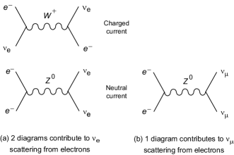
Figure 5: Feynman diagrams responsible for neutrino–electron scattering in a 2-flavor model with $\nu_{\mbox{\scriptsize e}}$ and $\nu_{\mu}$ flavors. Such diagrams are pictorial representations of quantum-mechanical matrix elements. For example, the upper left diagram stands for the matrix element ($\sim$ probability amplitude) for a process where an electron neutrino exchanges a virtual $W^{+}$ intermediate vector boson with an electron, with the neutrino converted to an electron and the electron converted to an electron neutrino. This is a charged-current process, because the $W^{+}$ virtual exchange particle is electrically charged. On the other hand, the lower left diagram describes a neutral-current process where the exchanged virtual $Z^{0}$ carries no electrical charge. Electron neutrinos can interact with electrons through both the charged-current and neutral-current diagrams shown in (a), but muon and tau neutrinos can interact with electrons only through the neutral-current diagram in (b).

The neutral current interaction contributes to both electron and muon neutrino scattering, so let’s ignore it and concentrate on the charged-current diagram in Fig. 5(a) that contributes only to $\nu_{\mbox{\scriptsize e}}$ elastic scattering in a 2-flavor model. From standard methods of quantum field theory kuo1989 ; smir2003 ; blen2013 the charged-current diagram in Fig. 5 contributes a medium-dependent interaction having the form of an effective potential energy $V$ seen only by the electron neutrinos or antineutrinos, with a magnitude

$$V=\pm\sqrt{2}G_{\mbox{\scriptsize F}}n_{\mbox{\scriptsize e}},$$ (13)

where the positive sign is for electron neutrinos (our primary concern here), the negative sign is for electron antineutrinos, $n_{\mbox{\scriptsize e}}$ is the local electron number density, and $G_{\mbox{\scriptsize F}}$ is the weak (Fermi) coupling constant characterizing the strength of the weak interactions. The energy is given by $E^{2}=p^{2}+m^{2}$. For the electron neutrino subject to the additional potential $V$

$$p^{2}+m^{2}=(E-V)^{2}=E^{2}\left(1-\frac{V}{E}\right)^{2}\simeq E^{2}-2EV,$$ (14)

where the last step is justified by assuming that $V{\ \scriptstyle<<\ }E$. Thus

$$E^{2}\sim p^{2}+(m^{2}+2EV).$$ (15)

Since $V$ is positive, an electron neutrino behaves effectively as if it is slightly heavier when propagating through matter than in vacuum, with the amount of increase governed by the electron density of the matter, but a muon or tau neutrino is unaffected because they do not see the effective potential $V$. Fig. 6 illustrates.

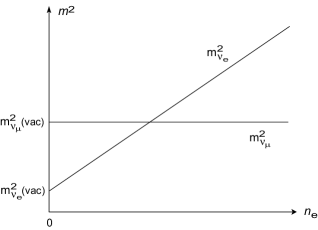
Figure 6: The effective mass-squared of electron neutrinos and muon neutrinos as a function of electron number density $n_{\mbox{\scriptsize e}}$, neglecting flavor mixing. Because the $\nu_{\mu}$ does not couple to the charged weak current its $m^{2}$ does not depend on $n_{\mbox{\scriptsize e}}$ but the effective $m^{2}$ of $\nu_{\mbox{\scriptsize e}}$ increases linearly with the electron density. Thus the $m^{2}$ spectrum in vacuum can be inverted in matter at high electron density.

From this figure, an electron neutrino that is less massive than a muon neutrino in vacuum will become effectively more massive than its oscillation partner in matter if the electron density is sufficiently high.

IV.2 The Mass Matrix

To address in more depth neutrino oscillations in matter, let’s introduce a more formal derivation of the neutrino oscillation problem that will prove to be useful for subsequent discussion. bah89 ; wol78 ; bet86 ; kuo1989 ; col89b ; mori2004

IV.2.1 Propagation of Left-Handed Neutrinos

First note that the full spin structure does not influence the propagation of neutrinos in the absence of magnetic fields because only the left-handed component of the neutrino couples to the weak interactions. The Schrödinger equation of ordinary quantum mechanics is not relativistically invariant and so is not appropriate for relativistic particles. For relativistic fermions the wave equation must be generalized to the Dirac equation, while for spinless particles the corresponding relativistic wave equation is the Klein–Gordon equation. Relativistic fermions are generally described by a Dirac equation but if the spin structure is eliminated from consideration the propagation of a (left-handed component of the) free neutrino may instead be described by the simpler free-particle Klein–Gordon equation

$$({\Box}+m^{2})|\nu\rangle=0\qquad{\Box}\equiv-\frac{\partial^{2}}{\partial t^{2}}+\frac{\partial^{2}}{\partial x^{2}}+\frac{\partial^{2}}{\partial y^{2}}+\frac{\partial^{2}}{\partial z^{2}},$$ (16)

where ${\Box}$ is termed the d’Alembertian operator and for $n$ neutrino flavors $|\nu\rangle$ is an $n$-component column vector in the mass-eigenstate basis and $m^{2}$ is an $n\times n$ matrix.

Because of oscillations, the solutions to Eq. (16) of interest correspond to the propagation of a linear combination of mass eigenstates. For ultrarelativistic neutrinos one makes only small errors by assuming neutrinos of tiny mass and slightly different energies to propagate with the same 3-momentum $\bm{p}$. In that approximation a solution of Eq. (16) for definite momentum is given by

$$|\nu_{i}\rangle=e^{-iE_{i}t}\cdot e^{-i\bm{p}\cdot\bm{x}}\qquad E_{i}=\sqrt{\bm{p}^{2}+m_{i}^{2}}.$$ (17)

For ultrarelativistic particles $|\bm{p}|{\ \scriptstyle>>\ }m_{i}$ so

$$E_{i}=\left[\bm{p}^{2}\left(1+\frac{m_{i}^{2}}{\bm{p}^{2}}\right)\right]^{1/2}\simeq\,\bm{p}+\frac{m_{i}^{2}}{2|\bm{p}|}\simeq\,\bm{p}+\frac{m_{i}^{2}}{2E},$$ (18)

where $E\sim p\equiv|\bm{p}|$. Thus, from Eq. (17)

$$|\nu_{i}(t)\rangle\,\simeq\,e^{-i|\bm{p}|t}\cdot e^{-i\bm{p}\cdot\bm{x}}e^{-i\bm{p}\cdot\bm{x}}\cdot e^{-i(m_{i}^{2}/2E)t}.$$

But the initial exponential factors involving the 3-momenta provide only a common overall phase that does not affect observables, so they may be dropped to give

$$|\nu_{i}(t)\rangle\simeq\,e^{-i(m_{i}^{2}/2E)t}.$$ (19)

Differentiating Eq. (19) with respect to time gives an equation of motion for a single mass eigenstate labeled by $i$,

$$i\,\frac{d}{dt}\,|\nu_{i}(t)\rangle=\frac{m_{i}^{2}}{2E}\,|\nu_{i}(t)\rangle,$$ (20)

which may be generalized for a 2-flavor model to the matrix equation

$$i\,\frac{d}{dt}\begin{pmatrix}\nu_{1}\\ \nu_{2}\end{pmatrix}=\begin{pmatrix}m_{1}^{2}/2E&0\\ 0&m_{2}^{2}/2E\end{pmatrix}\begin{pmatrix}\nu_{1}\\ \nu_{2}\end{pmatrix},$$ (21)

where the quantity

$$M\equiv\begin{pmatrix}m_{1}^{2}/2E&0\\ 0&m_{2}^{2}/2E\end{pmatrix}$$

is termed the mass matrix. In these equations elapsed time $t$ or distance traveled $r$ may be used interchangeably as the independent variable, since $r\sim ct$ for ultrarelativistic neutrinos.

IV.2.2 Evolution in the Flavor Basis

Neutrinos propagate in mass eigenstates but they are produced and detected in flavor eigenstates, so it is useful to express the preceding equation in the flavor basis. The transformations matrices are given in Eqs. (2) and (3), which permits Eq. (21) to be written in the form

$$i\,\frac{d}{dt}\begin{pmatrix}\nu_{1}\\ \nu_{2}\end{pmatrix} =i\,\frac{d}{dt}\,U^{\dagger}\begin{pmatrix}\nu_{\mbox{\scriptsize e}}\\ \nu_{\mu}\end{pmatrix}$$

$$=\begin{pmatrix}m_{1}^{2}/2E&0\\ 0&m_{2}^{2}/2E\end{pmatrix}U^{\dagger}\begin{pmatrix}\nu_{\mbox{\scriptsize e}}\\ \nu_{\mu}\end{pmatrix}.$$

Multiplying from the left by $U$ and using the unitarity condition $UU^{\dagger}=1$ gives

$$i\,\frac{d}{dt}\begin{pmatrix}\nu_{\mbox{\scriptsize e}}\\ \nu_{\mu}\end{pmatrix}=U\begin{pmatrix}m_{1}^{2}/2E&0\\ 0&m_{2}^{2}/2E\end{pmatrix}U^{\dagger}\begin{pmatrix}\nu_{\mbox{\scriptsize e}}\\ \nu_{\mu}\end{pmatrix},$$ (22)

where the flavor and mass eigenstates are related by

$$\begin{pmatrix}\nu_{\mbox{\scriptsize e}}\\ \nu_{\mu}\end{pmatrix}=U\begin{pmatrix}\nu_{1}\\ \nu_{2}\end{pmatrix}\qquad\begin{pmatrix}\nu_{1}\\ \nu_{2}\end{pmatrix}=U^{\dagger}\begin{pmatrix}\nu_{\mbox{\scriptsize e}}\\ \nu_{\mu}\end{pmatrix},$$

and the transformation matrices between mass and flavor bases may be written explicitly as

$$U=\begin{pmatrix}\cos\theta&\sin\theta\\ -\sin\theta&\cos\theta\end{pmatrix}\qquad U^{\dagger}=\begin{pmatrix}\cos\theta&-\sin\theta\\ \sin\theta&\cos\theta\end{pmatrix}.$$

As is clear by substitution, Eq. (22) has a solution

$$\begin{pmatrix}\nu_{\mbox{\scriptsize e}}(t)\\ \nu_{\mu}(t)\end{pmatrix}=U\begin{pmatrix}e^{-i(m_{1}^{2}/2E)t}&0\\ 0&e^{-i(m_{2}^{2}/2E)t}\end{pmatrix}U^{\dagger}\begin{pmatrix}\nu_{\mbox{\scriptsize e}}(0)\\ \nu_{\mu}(0)\end{pmatrix}.$$

Since no individual neutrino mass has been measured thus far, it is convenient to rewrite Eq. (22) in terms of $\Delta m^{2}$, which has been measured. Adding a multiple of the unit matrix to the matrix in Eq. (22) will not modify quantum observables (a trick that will be employed several times in what follows), so let’s subtract $m_{1}^{2}/2E$ times the unit $2\times 2$ matrix from the matrix in Eq. (22) and use

$$\begin{pmatrix}0&0\\ 0&\Delta m^{2}/2E\end{pmatrix}=\begin{pmatrix}m_{1}^{2}/2E&0\\ 0&m_{2}^{2}/2E\end{pmatrix}-\begin{pmatrix}m_{1}^{2}/2E&0\\ 0&m_{1}^{2}/2E\end{pmatrix}$$

to replace Eq. (22) by the equivalent form

$$i\,\frac{d}{dt}\begin{pmatrix}\nu_{\mbox{\scriptsize e}}\\ \nu_{\mu}\end{pmatrix}=U\begin{pmatrix}0&0\\ 0&\Delta m^{2}/2E\end{pmatrix}U^{\dagger}\begin{pmatrix}\nu_{\mbox{\scriptsize e}}\\ \nu_{\mu}\end{pmatrix},$$ (23)

where the mass-squared difference $\Delta m^{2}\equiv m_{2}^{2}-m_{1}^{2}$ was introduced in Eq. (9).

IV.2.3 Propagation in Matter

The flavor evolution equation (23) is just a reformulation of our previous treatment of neutrinos propagating in vacuum, so it contains nothing new. However, let us now add a charged-current interaction with matter. By previous arguments the charged current couples only elastically and only to electron neutrinos, so we add to the Klein–Gordon equation (16) an interaction potential given by Eq. (13), which modifies the equation of motion (23) to

$$i\,\frac{d}{dt}\begin{pmatrix}\nu_{\mbox{\scriptsize e}}\\ \nu_{\mu}\end{pmatrix}=\left[U\begin{pmatrix}0&0\\ 0&\Delta m^{2}/2E\end{pmatrix}U^{\dagger}+\begin{pmatrix}V(t)&0\\ 0&0\end{pmatrix}\right]\begin{pmatrix}\nu_{\mbox{\scriptsize e}}\\ \nu_{\mu}\end{pmatrix},$$

where the effective potential generated by the charged-current coupling of the electron neutrino to the matter,

$$V(t)=\sqrt{2}G_{\mbox{\scriptsize F}}\,n_{\mbox{\scriptsize e}}(t),$$ (24)

depends on time (or equivalently on position), because it is a function of the electron density. Inserting the explicit forms for the transformation matrices $U$ and $U^{\dagger}$ gives

$$i\,\frac{d}{dt}\begin{pmatrix}\nu_{\mbox{\scriptsize e}}\\ \nu_{\mu}\end{pmatrix}=$$

$$\left[\begin{pmatrix}\cos\theta&\sin\theta\\ -\sin\theta&\cos\theta\end{pmatrix}\begin{pmatrix}0&0\\ 0&\Delta m^{2}/2E\end{pmatrix}\begin{pmatrix}\cos\theta&-\sin\theta\\ \sin\theta&\cos\theta\end{pmatrix}\right.$$

$$\left.\quad+\begin{pmatrix}V&0\\ 0&0\end{pmatrix}\right]\begin{pmatrix}\nu_{\mbox{\scriptsize e}}\\ \nu_{\mu}\end{pmatrix}$$

$$=\left[\begin{pmatrix}{\dfrac{\Delta m^{2}}{2E}\sin^{2}\theta}&{\dfrac{\Delta m^{2}}{2E}\sin\theta\cos\theta}\\[6.0pt] {\dfrac{\Delta m^{2}}{2E}\sin\theta\cos\theta}&{\dfrac{\Delta m^{2}}{2E}\cos^{2}\theta}\end{pmatrix}+\begin{pmatrix}V&0\\ 0&0\end{pmatrix}\right]\begin{pmatrix}\nu_{\mbox{\scriptsize e}}\\ \nu_{\mu}\end{pmatrix}$$

$$=\left[\frac{\Delta m^{2}}{2E}\begin{pmatrix}0&\sin\theta\cos\theta\\ \sin\theta\cos\theta&\cos^{2}\theta-\sin^{2}\theta\end{pmatrix}+\begin{pmatrix}V&0\\ 0&0\end{pmatrix}\right]\begin{pmatrix}\nu_{\mbox{\scriptsize e}}\\ \nu_{\mu}\end{pmatrix}$$

$$=\begin{pmatrix}{V}&{\dfrac{\Delta m^{2}}{4E}\sin 2\theta}\\[6.0pt] {\dfrac{\Delta m^{2}}{4E}\sin 2\theta}&{\dfrac{\Delta m^{2}}{2E}\cos 2\theta}\end{pmatrix}\begin{pmatrix}\nu_{\mbox{\scriptsize e}}\\ \nu_{\mu}\end{pmatrix}\equiv M\begin{pmatrix}\nu_{\mbox{\scriptsize e}}\\ \nu_{\mu}\end{pmatrix},$$ (25)

where in the second step $(\Delta m^{2}/4E)\sin^{2}\theta$ times the $2\times 2$ unit matrix has been subtracted, in the final line the trigonometric identities

$$\sin\theta\cos\theta=\tfrac{1}{2}\sin 2\theta\qquad\cos^{2}\theta-\sin^{2}\theta=\cos 2\theta$$

have been used, and $M$ is termed the mass matrix (in the flavor basis).

Eq. (25) is the required result but it is conventional to write the mass matrix $M$ appearing in it in a more symmetric form. First define

$$A\equiv 2EV=2\sqrt{2}EG_{\mbox{\scriptsize F}}n_{\mbox{\scriptsize e}},$$ (26)

(which has units of mass squared) and then subtract $A/4E+(\Delta m^{2}/4E)\cos 2\theta$ multiplied by the unit matrix to give the mass matrix in traceless form

$$\begin{split}M&=\frac{\Delta m^{2}}{4E}\begin{pmatrix}\dfrac{A}{\Delta m^{2}}-\cos 2\theta&\sin 2\theta\\ \sin 2\theta&\cos 2\theta-\dfrac{A}{\Delta m^{2}}\end{pmatrix}\\ &=\displaystyle\frac{\pi}{L}\begin{pmatrix}\chi-\cos 2\theta&\sin 2\theta\\ \sin 2\theta&\cos 2\theta-\chi\end{pmatrix},\end{split}$$ (27)

where the dimensionless charged-current coupling strength $\chi$ has been introduced through

$$\chi\equiv\frac{L}{\ell_{\mbox{\scriptsize m}}}=\frac{2EV}{\Delta m^{2}}\qquad\ell_{\mbox{\scriptsize m}}\equiv\frac{\sqrt{2}\pi}{G_{\mbox{\scriptsize F}}n_{\mbox{\scriptsize e}}}\qquad L\equiv\frac{4\pi E}{\Delta m^{2}},$$ (28)

with $L$ the vacuum oscillation length defined in Eq. (11) and $\ell_{\mbox{\scriptsize m}}$ an additional contribution to the oscillation length in matter that is termed the refraction length because it is a characteristic distance over which there is significant refraction of the neutrino by the matter. smir2003

IV.3 Solutions in Matter

For a fixed density the mass eigenstates in matter—which generally will differ from the mass eigenstates in vacuum because of the interaction $V$—may be found by diagonalizing (finding the eigenvalues) of the mass matrix $M$ at that density. However, since the interaction $V$ depends on the density, in a medium with varying density such as the Sun the mass eigenstates in matter at one time (or position) will generally not be eigenstates at another time. Let’s imagine dividing the Sun up into concentric radial layers, as illustrated in Fig. 7,

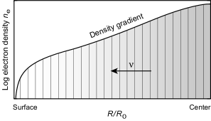
Figure 7: Solar density gradient. Neutrinos are produced near the center at high density and propagate out through regions of decreasing density. Within a given concentric layer, the density may be assumed to be nearly constant.

and assume the density within each layer to be approximately constant. Our approach will be to first understand how to calculate the mass eigenstates within a single layer assumed to have a constant density, and then to determine the evolution of neutrino states as they propagate through successive layers of decreasing density in the Sun.

IV.3.1 Mass Eigenvalues for Constant Density

At constant density the problem resembles vacuum oscillations, except with a different potential $V\neq 0$, and the time-evolved mass states in matter, $|\nu_{\scriptscriptstyle 1}^{\scriptscriptstyle\rm m}\rangle$ and $|\nu_{\scriptscriptstyle 2}^{\scriptscriptstyle\rm m}\rangle$, may be found by determining the eigenvalues of the mass matrix (27). The eigenvalues of an $n\times n$ matrix $A$ correspond to the values of $\lambda$ that solve the characteristic equation $\det(A-\lambda I)=0,$ with $I$ the $n\times n$ unit matrix and $\det$ indicating the determinant. For a general $2\times 2$ matrix

$$A=\begin{pmatrix}\alpha&\beta\\ \gamma&\delta\end{pmatrix},$$

the characteristic equation is quadratic with the two solutions,

$$\lambda_{\pm}=\tfrac{1}{2}\mbox{tr}\thinspace(A)\pm\sqrt{\tfrac{1}{4}\mbox{tr}\thinspace(A)^{2}-\det(A)},$$

where $\mbox{tr}\thinspace A$ is the trace and $\det A$ is the determinant of $A$. Hence the eigenvalues $\lambda_{\pm}$ of the mass matrix (27) are given by

$$\begin{split}\lambda_{\pm}&=\left(\frac{m_{1}^{2}+m_{2}^{2}}{2}+\frac{\Delta m^{2}}{2}\chi\right)\\ &\quad\pm\frac{\Delta m^{2}}{2}\sqrt{(\cos 2\theta-\chi)^{2}+\sin^{2}2\theta}.\end{split}$$ (29)

The second term gives the splitting between the two mass eigenstates and is minimal at the density where $\chi=\cos 2\theta$. By analogy with the vacuum case, the mass eigenstates in matter, $\nu_{1}^{\rm m}\equiv|\nu_{\scriptscriptstyle 1}^{\scriptscriptstyle\rm m}\rangle$ and $\nu_{2}^{\rm m}\equiv|\nu_{\scriptscriptstyle 2}^{\scriptscriptstyle\rm m}\rangle$ at fixed time $t$, are assumed to be related to the flavor eigenstates by

$$\begin{pmatrix}\nu_{\mbox{\scriptsize e}}\\ \nu_{\mu}\end{pmatrix}=U_{\mbox{\scriptsize m}}(t)\begin{pmatrix}\nu_{1}^{\rm m}\\ \nu_{2}^{\rm m}\end{pmatrix}.$$ (30)

where $U_{\mbox{\scriptsize m}}(t)$ is a unitary matrix depending on the density that we must now determine.

IV.3.2 The Matter Mixing Angle $\bm{\theta_{\mbox{\scriptsize m}}}$

The matrix $U_{\mbox{\scriptsize m}}(t)$ can be parameterized as for the vacuum mixing matrix $U$, but now in terms of a time-dependent matter mixing angle $\theta_{\mbox{\scriptsize m}}(t)$ with

$$U_{\mbox{\scriptsize m}}=\begin{pmatrix}\cos\theta_{\mbox{\scriptsize m}}&\sin\theta_{\mbox{\scriptsize m}}\\ -\sin\theta_{\mbox{\scriptsize m}}&\cos\theta_{\mbox{\scriptsize m}}\end{pmatrix}\quad U_{\rm\scriptstyle m}^{\dagger}=\begin{pmatrix}\cos\theta_{\mbox{\scriptsize m}}&-\sin\theta_{\mbox{\scriptsize m}}\\ \sin\theta_{\mbox{\scriptsize m}}&\cos\theta_{\mbox{\scriptsize m}}\end{pmatrix}.$$ (31)

The relationship of the matter mixing angle $\theta_{\mbox{\scriptsize m}}$ and vacuum mixing angle $\theta$ at time $t$ can be established by requiring that a similarity transform by the unitary matrix $U_{\mbox{\scriptsize m}}(t)$ diagonalize the mass matrix, with the diagonal elements being the time-dependent eigenvalues in matter $E_{1}(t)$ and $E_{2}(t)$,

$$U_{\rm\scriptstyle m}^{\dagger}(t)MU_{\mbox{\scriptsize m}}(t)=\mbox{diag}\thinspace[E_{1}(t),E_{2}(t)]=\begin{pmatrix}E_{1}(t)&0\\ 0&E_{2}(t)\end{pmatrix}.$$ (32)

Inserting the explicit values of the matrices $U_{\mbox{\scriptsize m}}$, $U^{\dagger}_{\rm m}$, and $M$ from Eqs. (27) and (31) in Eq. (32) gives a matrix equation, for which comparison of matrix entries on the two sides of the equation requires the matter and vacuum mixing angles to be related by

$$\tan 2\theta_{\mbox{\scriptsize m}}=\frac{\sin 2\theta}{\cos 2\theta\pm\chi}=\frac{\tan 2\theta}{1\pm\chi/\cos 2\theta},$$ (33)

where the plus sign is for $m_{1}>m_{2}$ and the negative sign for $m_{1}<m_{2}$. From Eq. (33), in vacuum $\theta_{\mbox{\scriptsize m}}=\theta$ but in matter the mixing angle will be modified from its vacuum value by a density-dependent amount governed by the charged-current coupling strength $\chi$.

IV.3.3 The Matter Oscillation Length $\bm{L}_{\mbox{\scriptsize m}}$

From Eq. (11) the vacuum oscillation length is proportional to $1/\Delta m^{2}$. In matter the $\nu_{\mbox{\scriptsize e}}$ effective mass is altered by interaction with the medium and the vacuum mass-squared difference is rescaled, $\Delta m^{2}\rightarrow f(\chi)\Delta m^{2},$ where from the splitting of the two eigenvalues in Eq. (29)

$$f(\chi) =\sqrt{(\cos 2\theta-\chi)^{2}+\sin^{2}2\theta}$$

$$=\sqrt{1-2\chi\cos 2\theta+\chi^{2}}.$$ (34)

Hence the oscillation length in matter $L_{\mbox{\scriptsize m}}$ is given by

$$L_{\mbox{\scriptsize m}} =\frac{4\pi E}{f(\chi)\Delta m^{2}}=\frac{L}{f(\chi)}$$

$$=\frac{L}{\sqrt{(\cos 2\theta-\chi)^{2}+\sin^{2}2\theta}},$$ (35)

which reduces to the vacuum oscillation length $L$ if $\chi\rightarrow 0$. The variations of $\theta_{\mbox{\scriptsize m}}$, $L_{\mbox{\scriptsize m}}$, and $f$ with the dimensionless charged-current coupling strength $\chi$ are illustrated in Fig. 8

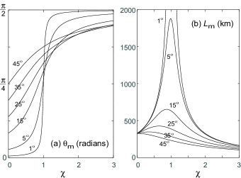
Figure 8: (a) Mixing angle in matter $\theta_{\mbox{\scriptsize m}}(\chi)$ and (b) oscillation length in matter $L_{\mbox{\scriptsize m}}(\chi)$, as a function of the dimensionless matter coupling parameter $\chi$. All calculations assumed $E=10\mbox{\ MeV}$ and $\Delta m^{2}=7.6\times 10^{-5}\mbox{\ eV}^{2}$, and curves are marked with the assumed vacuum mixing angle $\theta$.

for several values of the vacuum mixing angle $\theta$.

From Fig. 8(a), the matter mixing angle $\theta_{\mbox{\scriptsize m}}$ reduces to the vacuum mixing angle $\theta$ as $\chi\rightarrow 0$, but $\theta_{\mbox{\scriptsize m}}\rightarrow\frac{\pi}{2}$ for any value of the vacuum mixing angle as $\chi\rightarrow\infty$, with the rate of approach to $\tfrac{\pi}{2}$ being fastest for smaller vacuum angle. From Fig. 8(b) the matter oscillation length is equal to the vacuum oscillation length at zero coupling, but increases to a maximum at the coupling strength where $\theta_{\mbox{\scriptsize m}}=\frac{\pi}{4}$ [compare Fig. 8(a)], and then decreases again. The coupling strength at which $L_{\mbox{\scriptsize m}}$ is maximal coincides with highest rate of change in $\theta_{\mbox{\scriptsize m}}$, and with the minimum of the scaling function $f(\chi)$ displayed in Fig. 8(c). The rapid change of $\theta_{\mbox{\scriptsize m}}$ and the strong peaking of $L_{\mbox{\scriptsize m}}$ near the density where $\theta_{\mbox{\scriptsize m}}=\frac{\pi}{4}$ are suggestive of resonant behavior, as will be elaborated shortly.

IV.3.4 Flavor Conversion Probabilities in Constant-Density Matter

In constant-density matter the electron neutrino state after a time $t$ becomes

$$\begin{split}|\nu(t)\rangle=(\cos^{2}\theta_{\mbox{\scriptsize m}}e^{-iE_{1}t}+\sin^{2}\theta_{\mbox{\scriptsize m}}e^{-iE_{2}t})|\nu_{\mbox{\scriptsize e}}\rangle\\ +\sin\theta_{\mbox{\scriptsize m}}\cos\theta_{\mbox{\scriptsize m}}(-e^{-iE_{1}t}+e^{-iE_{2}t})|\nu_{\mu}\rangle,\end{split}$$ (36)

which is analogous to the vacuum equation Eq. (6) with $\theta$ replaced by $\theta_{\mbox{\scriptsize m}}$ defined through Eq. (33). The corresponding flavor conservation and retention probabilities are given by Eq. (10) with the replacements $\theta\rightarrow\theta_{\mbox{\scriptsize m}}$ and $L\rightarrow L_{\mbox{\scriptsize m}}$,

$$\begin{array}[]{c}P(\nu_{\mbox{\scriptsize e}}{\,\scriptstyle\rightarrow}\,\nu_{\mbox{\scriptsize e}},\,r)=1-\sin^{2}2\theta_{\mbox{\scriptsize m}}\sin^{2}\left(\displaystyle\frac{\pi r}{L_{\mbox{\scriptsize m}}}\right)\end{array}$$ (37)

with $P(\nu_{\mbox{\scriptsize e}}{\,\scriptstyle\rightarrow}\,\nu_{\mu},\,r)=1-P(\nu_{\mbox{\scriptsize e}}{\,\scriptstyle\rightarrow}\,\nu_{\mbox{\scriptsize e}},\,r)$. The corresponding classical averages are

$$\bar{P}(\nu_{\mbox{\scriptsize e}}{\,\scriptstyle\rightarrow\,}\nu_{\mbox{\scriptsize e}})=1-\tfrac{1}{2}\sin^{2}2\theta_{\mbox{\scriptsize m}}\quad\bar{P}(\nu_{\mbox{\scriptsize e}}{\,\scriptstyle\rightarrow\,}\nu_{\mu})=\tfrac{1}{2}\sin^{2}2\theta_{\mbox{\scriptsize m}},$$ (38)

which are appropriate when the uncertainty in distance between source and detection exceeds the oscillation length (which is generally the case for solar neutrinos).

IV.4 The MSW Resonance Condition

From Eq. (37), optimal flavor mixing occurs whenever $\sin^{2}2\theta_{\mbox{\scriptsize m}}\rightarrow 1$, implying that $|\theta_{\mbox{\scriptsize m}}|=\frac{\pi}{4}$. The most significant property of Eq. (33) relative to the vacuum solution is that if $\Delta m^{2}$ and $L$ are positive [requiring that $m_{1}<m_{2}$, which selects the negative sign in Eq. (33)]. Then $\tan 2\theta_{\mbox{\scriptsize m}}\rightarrow\pm\infty$ and $\theta_{\mbox{\scriptsize m}}\rightarrow\frac{\pi}{4}$ whenever

$$\chi=\cos 2\theta,$$ (39)

where $\chi=L/\ell_{\mbox{\scriptsize m}}$, as illustrated in Fig. 9.

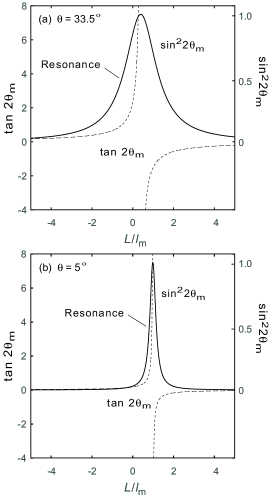
Figure 9: The MSW resonance condition for two values of the vacuum mixing angle $\theta$. When $\chi=L/\ell_{\mbox{\scriptsize m}}\rightarrow\cos 2\theta$ the denominator of Eq. (33) goes to zero, $\tan 2\theta_{\mbox{\scriptsize m}}$ goes to $\pm\infty$ so that $|\theta_{\mbox{\scriptsize m}}|\rightarrow\frac{\pi}{4}$, and the flavor conversion probability $\sin^{2}2\theta_{\mbox{\scriptsize m}}$ attains its maximum value. Thus, at the resonance Eq. (37) indicates that it is possible to obtain very large flavor conversion for any non-vanishing vacuum oscillation angle $\theta$.

From Eq. (28), this occurs when the electron density satisfies

$$n_{\mbox{\scriptsize e}}=\frac{\cos 2\theta\Delta m^{2}}{2\sqrt{2}G_{\mbox{\scriptsize F}}E}\equiv\mbox{$n_{\rm e}^{\rm\scriptscriptstyle R}$}.$$ (40)

From Eq. (37), this corresponds to a resonance condition leading to maximal flavor mixing between electron neutrinos and muon neutrinos, with a $\nu_{\mbox{\scriptsize e}}$ survival probability

$$P(\nu_{\mbox{\scriptsize e}}{\,\scriptstyle\rightarrow}\,\nu_{\mbox{\scriptsize e}},\,r)=1-\sin^{2}\left(\frac{\pi r}{L_{\mbox{\scriptsize m}}}\right)\qquad{\rm(at\ resonance)},$$ (41)

and, from Eqs. (35) and (39), an oscillation length at resonance $L_{\scriptscriptstyle\rm m}^{\rm\scriptscriptstyle R}$ given by

$$L_{\scriptscriptstyle\rm m}^{\rm\scriptscriptstyle R}=L_{\mbox{\scriptsize m}}(\chi=\cos 2\theta)=\frac{L}{\sin 2\theta}.$$ (42)

This is the Mikheyev–Smirnov–Wolfenstein or MSW resonance. wol78 ; mik86 It implies that—no matter how small the vacuum mixing angle $\theta$—as long as it is not zero there is some critical value $n_{\rm e}^{\rm\scriptscriptstyle R}$ of the electron density defined by Eq. (40) where the resonance condition is satisfied and maximal flavor mixing ensues. The important resonance parameters are plotted in Fig. 10

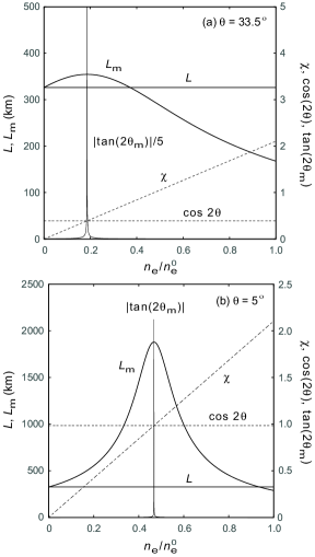
Figure 10: Resonance parameters versus the electron number density $n_{\mbox{\scriptsize e}}$ in units of the central solar value $n_{\rm\scriptstyle e}^{0}\sim 6.3\times 10^{25}\mbox{\ cm}^{-3}$ for $\theta=33.5^{\circ}$ and $5^{\circ}$, with $\Delta m^{2}=7.6\times 10^{-5}\mbox{\ eV}^{2}$ and $E=10\mbox{\ MeV}$. The coupling strength $\chi=L/\ell_{\mbox{\scriptsize m}}$ is linear in the density. Intersection of the dashed lines specifies the density giving the resonance condition.

as a function of electron density for two values of the vacuum mixing angle $\theta$.

The effect of the MSW resonance on variation of the matter mixing angle $\theta_{\mbox{\scriptsize m}}$ and the oscillation length in matter $L_{\mbox{\scriptsize m}}$ are illustrated for a small and large angle solution in Fig. 11.

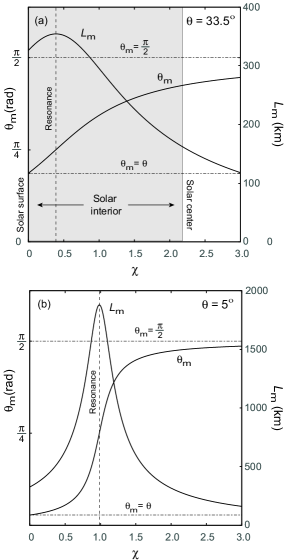
Figure 11: Matter mixing angle $\theta_{\mbox{\scriptsize m}}$ as a function of the dimensionless coupling strength $\chi\equiv L/\ell_{\mbox{\scriptsize m}}$ for vacuum mixing angles of (a) $\theta=33.5^{\circ}$ and (b) $\theta=5^{\circ}$. Also shown is the matter oscillation length $L_{\mbox{\scriptsize m}}$, which has a maximum at the MSW resonance (see Section IV.4), marked by the dashed vertical line. The oscillation length was computed from Eqs. (35) and (11) assuming $E=10\mbox{\ MeV}$ and $\Delta m^{2}=7.6\times 10^{-5}\mbox{\ eV}^{2}$. Case (a) is realistic for solar neutrinos and at the center of the Sun $\chi\sim 2.13$. Hence the shaded region on the left side of (a) indicates the range of coupling strengths available to electron neutrinos in the interior of the Sun.

The values of $\theta_{\mbox{\scriptsize m}}$ and $L_{\mbox{\scriptsize m}}$ will vary with the solar depth since they depend on the number density $n_{\mbox{\scriptsize e}}$ through $\chi$. From Eq. (33), $\theta_{\mbox{\scriptsize m}}\rightarrow\theta$ as the electron density tends to zero, while in the opposite limit of very large electron density $\theta_{\mbox{\scriptsize m}}\rightarrow\tfrac{\pi}{2}$. From Fig. 11, the manner in which the two limits are approached depends on whether the vacuum mixing angle is large or small. Case (a) corresponds to parameters valid for solar neutrinos. At the solar center (where $\chi\sim 2.13$) the value of the matter mixing angle is $\theta_{\mbox{\scriptsize m}}\sim 76^{\circ}$, compared with a vacuum mixing angle $33.5^{\circ}$ at the solar surface. Conversely, for case (b) with $\theta=5^{\circ}$ at the solar surface, the matter mixing angle at a density corresponding to the solar center is $\theta\sim 86^{\circ}$.

IV.5 Resonance in the Antineutrino Channel

If the condition $m_{1}<m_{2}$ is not satisfied there is no MSW resonance for electron neutrinos in a 2-flavor model; there is instead a corresponding resonance condition for the electron antineutrino $\bar{\nu}_{\mbox{\scriptsize e}}$. Antineutrino oscillations could be important in environments such as core-collapse supernovae where all flavors of neutrinos and antineutrinos are found in copious amounts, but the Sun produces mostly neutrinos so consideration of oscillations for antineutrinos will be omitted from the present discussion.

IV.6 Resonant Flavor Conversion

If $m_{1}<m_{2}$ and the electron density in the central region of the Sun where neutrinos are produced satisfies $n_{\mbox{\scriptsize e}}>\mbox{$n_{\rm e}^{\rm\scriptscriptstyle R}$}$, a solar neutrino will inevitably encounter the MSW resonance on its way out of the Sun. If the change in density is sufficiently slow that the additional phase mismatch between the $\nu_{\mbox{\scriptsize e}}$ and $\nu_{\mu}$ components produced by the charged-current elastic scattering from electrons changes very slowly with density (the adiabatic condition discussed further below), the $\nu_{\mbox{\scriptsize e}}$ flux produced in the core can be almost entirely converted to $\nu_{\mu}$ by the MSW resonance near the radius where the condition (40) is satisfied.

MSW flavor conversion can be viewed as an adiabatic quantum level crossing, bet86 ; hax86 as illustrated schematically in Fig. 12,

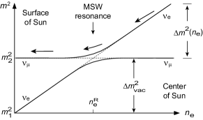
Figure 12: Schematic illustration of resonance flavor conversion as an adiabatic quantum level crossing. Specific examples for different parameter choices are shown in Fig. 13.

and more realistically in Fig. 13.

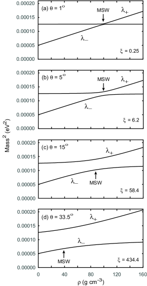
Figure 13: Solutions $\lambda_{\pm}$ of the MSW eigenvalue problem as a function of mass density according to Eq. (29). Each case corresponds to the choices $\Delta m^{2}=7.6\times 10^{-5}\mbox{\ eV}^{2}$ and $E=10\mbox{\ MeV}$, but to different values of the vacuum mixing angle $\theta$. The individual neutrino masses are presently unknown but for purposes of illustration $m_{1}^{2}=5\times 10^{-5}\mbox{\ eV}^{2}$ has been assumed in vacuum, so that $m_{2}^{2}=m_{1}^{2}+\Delta m^{2}=1.26\times 10^{-4}\mbox{\ eV}^{2}$. The critical density leading to the MSW resonance (corresponding to minimum splitting between the eigenvalues) and the value of the adiabaticity parameter $\xi=\delta r_{\rm\scriptscriptstyle R}/L^{\rm\scriptscriptstyle R}_{\rm\scriptscriptstyle m}$ defined in Eq. (45) are indicated for each case. As will be discussed in Section V, realistic solar conditions imply the highly adiabatic crossing exhibited in case (d).

Solutions of the MSW eigenvalue problem illustrating this level crossing for various choices of the vacuum mixing angle are displayed in Fig. 13. At zero density on the left side of these plots the eigenvalues $\lambda_{\pm}$ converge to the vacuum $m^{2}$ values, but for non-zero density the masses are altered by the interaction of the electron neutrino with the medium and the mixing of the solutions by the neutrino oscillation. (Compare with the unmixed case in Fig. 6.)

A neutrino produced near the center of the Sun (high density on right side) will be in a $\nu_{\mbox{\scriptsize e}}$ flavor eigenstate that coincides with the higher-mass eigenstate, since $V$ representing interaction with the medium increases the mass of the electron neutrino but not the muon neutrino. As the neutrino propagates out of the Sun (right to left in this diagram) the density decreases so $V$ and the effective mass of the neutrino decrease. Conversely, the lower-mass eigenstate (primarily $\nu_{\mu}$ flavor) remains constant in mass as $n_{\mbox{\scriptsize e}}$ decreases (no coupling to the charged current). Thus the two levels cross at the critical density where the effect of $V$ exactly cancels the vacuum mass-squared difference $\Delta m^{2}_{\rm\scriptstyle vac}\equiv\Delta m^{2}(n_{\mbox{\scriptsize e}}=0)$ between the eigenstates, and the neutrino remains in the high-mass eigenstate and changes adiabatically into a $\nu_{\mu}$ flavor state by the time it exits the Sun (left side), because in vacuum the high-mass eigenstate approximately coincides with $\nu_{\mu}$.

In summary, if the crossing is adiabatic the neutrino remains in the high-mass eigenstate in which it was created and follows the upper curved trajectory though the resonance in the level-crossing region, as indicated by the arrows. It emerges from the Sun in a different flavor state than the one in which it was created in the core of the Sun because the high-mass eigenstate is primarily $\nu_{\mbox{\scriptsize e}}$ in the dense medium but is primarily $\nu_{\mu}$ in vacuum. Such adiabatic crossing of energy levels is common in a variety of quantum systems and is often termed avoided level crossing.

The number density of electrons in the Sun computed in the Standard Solar Model is illustrated in Fig. 2, along with an exponential approximation that is rather good in the region of the Sun where the MSW effect is most important. In Fig. 14,

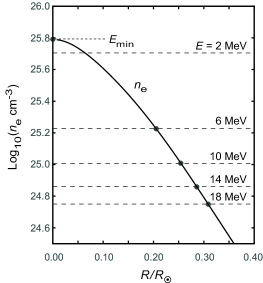
Figure 14: Radius where the MSW critical density for a 2-flavor model is realized (dots at intersection of dashed lines with the curve for $n_{\mbox{\scriptsize e}}$) for neutrinos of energies ranging from 2 to 18 MeV. A vacuum mixing angle $\theta=35^{\circ}$ and $\Delta m^{2}c^{4}=7.5\times 10^{-5}\mbox{\ eV}^{2}$ have been assumed. The minimum energy of an electron neutrino $E_{\mbox{\scriptsize min}}\sim 1.6\mbox{\ MeV}$ that could be produced in the Sun and still encounter the MSW resonance is indicated.

the approximate locations in the Sun where electron neutrinos of various energies would encounter the MSW resonance condition [determined by solving Eq. (40) for each choice of energy] are illustrated. Only neutrinos having an energy larger than some minimum energy $E_{\mbox{\scriptsize min}}$ can experience the MSW resonance in the Sun because the neutrino must be produced at a density higher than the critical resonance density. The conditions used to obtain Fig. 14 give $E_{\mbox{\scriptsize min}}\sim 1.6\mbox{\ MeV}$. Thus, we may expect that the MSW effect is more efficient at converting the flavor of higher-energy neutrinos. That flavor conversion is observed to be preferentially suppressed for lower-energy solar neutrinos will be an important piece of evidence favoring the MSW mechanism over vacuum oscillations for the observed flavor conversion of solar neutrinos.

IV.7 Neutrino Propagation in Matter with Varying Density

Consider now realistic neutrino propagation in the Sun, where a neutrino produced in the core will encounter steadily decreasing density as it travels toward the solar surface (see Fig. 7). The neutrino flavor evolution will be governed by the analog of the coupled differential equations for vacuum propagation, but with $U\rightarrow U_{\mbox{\scriptsize m}}(t)$ since the flavor–mass basis transformation now depends on time. From Eq. (22) with this replacement

$$i\,\frac{d}{dt}\left[U_{\mbox{\scriptsize m}}(t)\begin{pmatrix}\nu_{1}(t)\\ \nu_{2}(t)\end{pmatrix}\right]=\frac{1}{2E}\,U_{\mbox{\scriptsize m}}(t)\begin{pmatrix}m_{1}^{2}&0\\ 0&m_{2}^{2}\end{pmatrix}\begin{pmatrix}\nu_{1}(t)\\ \nu_{2}(t)\end{pmatrix},$$

where both the wavefunctions and the transformation matrix $U_{\mbox{\scriptsize m}}$ are indicated explicitly to depend on the time. Taking the time derivative of the product in brackets on the left side and multiplying the equation from the left by $U_{\rm\scriptstyle m}^{\dagger}$ gives

$$i\frac{d}{dt}\begin{pmatrix}\nu_{1}\\ \nu_{2}\end{pmatrix} =\left[\begin{pmatrix}m_{1}^{2}/2E&0\\ 0&m_{2}^{2}/2E\end{pmatrix}-i\,U^{\dagger}_{\rm\scriptstyle m}\,\frac{d}{dt}\,U_{\mbox{\scriptsize m}}\right]\begin{pmatrix}\nu_{1}\\ \nu_{2}\end{pmatrix}$$

$$=\begin{pmatrix}m_{1}^{2}/2E&-i\dot{\theta}_{\mbox{\scriptsize m}}\\ i\dot{\theta}_{\mbox{\scriptsize m}}&m_{2}^{2}/2E\end{pmatrix}\begin{pmatrix}\nu_{1}\\ \nu_{2}\end{pmatrix}$$

$$=\begin{pmatrix}-\Delta m^{2}/4E&-i\,\dot{\theta}_{\mbox{\scriptsize m}}\\ i\,\dot{\theta}_{\mbox{\scriptsize m}}&\Delta m^{2}/4E\end{pmatrix}\begin{pmatrix}\nu_{1}\\ \nu_{2}\end{pmatrix},$$ (43)

where Eq. (31) was used, $\dot{\theta}_{\mbox{\scriptsize m}}\equiv d\theta_{\mbox{\scriptsize m}}/dt$, and in the last step the constant $(m_{1}^{2}+m_{2}^{2})/4E$ times the unit matrix has been subtracted from the matrix on the right side (which does not affect observables).

Our earlier statement that mass eigenstates at some density in the Sun generally will not be eigenstates at a different density may now be quantified. If the mass matrix in Eq. (43) were diagonal the neutrino would remain in its original mass eigenstate as it traveled through regions of varying density, so it is the off-diagonal terms proportional to $\dot{\theta}_{\mbox{\scriptsize m}}=d\theta_{\mbox{\scriptsize m}}/dt$ that alter the mass eigenstates as the neutrino propagates. Generally then, Eq. (43) must be solved numerically. However, if the off-diagonal terms are small relative to the diagonal terms, the mass matrix $M$ may be approximated by dropping the off-diagonal terms

$$M=\begin{pmatrix}-\Delta m^{2}/4E&-i\,\dot{\theta}_{\mbox{\scriptsize m}}\\ i\,\dot{\theta}_{\mbox{\scriptsize m}}&\Delta m^{2}/4E\end{pmatrix}\simeq\frac{\Delta m^{2}}{4E}\begin{pmatrix}-1&0\\ 0&1\end{pmatrix},$$ (44)

which affords the possibility of an analytical solution for neutrino flavor conversion in the Sun. This is called the adiabatic approximation, and corresponds physically to the assumption that the matter mixing angle $\theta_{\mbox{\scriptsize m}}$ changes only slowly over a characteristic time for motion of the neutrino. A neutrino travels at near light speed so $r\sim ct$ and the adiabatic condition also may be interpreted as a limit on the spatial gradient of $\theta_{\mbox{\scriptsize m}}$. From Fig. 8(a) and Fig. 11, the most rapid change in $\theta_{\mbox{\scriptsize m}}$ and thus the largest contribution of the off-diagonal terms occurs near the MSW resonance (corresponding to $\theta_{\mbox{\scriptsize m}}=\frac{\pi}{4}$). Let us now use these observations to quantify the conditions appropriate for the adiabatic approximation.

IV.8 The Adiabatic Criterion

The adiabatic condition for resonant flavor conversion can be expressed as a requirement that the spatial width of the resonance layer $\delta r_{\rm\scriptscriptstyle R}$ (which is defined by the radial distance over which the resonance condition is approximately fulfilled) be much greater than the oscillation wavelength in matter evaluated at the resonance, $L^{\rm\scriptscriptstyle R}_{\rm\scriptscriptstyle m}$. This can be characterized by introducing an adiabaticity parameter $\xi$ through the definition [see Eq. (42)]

$$\xi\equiv\frac{\delta r_{\rm\scriptscriptstyle R}}{L^{\rm\scriptscriptstyle R}_{\rm\scriptscriptstyle m}}\quad\delta r_{\rm\scriptscriptstyle R}=\frac{\mbox{$n_{\rm e}^{\rm\scriptscriptstyle R}$}}{(dn_{\mbox{\scriptsize e}}/dr)_{\rm\scriptscriptstyle R}}\tan 2\theta\quad L^{\rm\scriptscriptstyle R}_{\rm\scriptscriptstyle m}=\frac{L}{\sin 2\theta},$$ (45)

where an index R labels quantities that are evaluated at the resonance, $L$ is the vacuum oscillation length, and $\theta$ is the vacuum oscillation angle. bet86 ; smir2003 The adiabatic condition corresponds then to the requirement that $\xi{\ \scriptstyle>>\ }1$, which implies physically that if many flavor oscillation lengths (in matter) fit within the resonance layer the adiabatic approximation of Eq. (44) is valid.

Values of $\xi$ computed from Eq. (45) are indicated in Fig. 13 for several choices of vacuum mixing angle $\theta$. In general very sharp level crossings as in Fig. 13(a) are non-adiabatic, while avoided level crossings as in Fig. 13(d) are highly adiabatic. In the limit of no mixing ($\theta=0$) the levels cross with no interaction, as illustrated earlier in Fig. 6. From Fig. 13 one sees that the MSW resonance can occur under approximately adiabatic conditions, even for relatively small values of the vacuum mixing angle [for example, case (b)]. As will be shown in Section V, solar conditions correspond to the highly-avoided level crossing in Fig. 13(d), for which $\delta r_{\rm\scriptscriptstyle R}{\ \scriptstyle>>\ }L^{\rm\scriptscriptstyle R}_{\rm\scriptscriptstyle m}$. Thus the MSW resonance is expected to be encountered adiabatically in the Sun, which optimizes the chance of resonant flavor conversion.

IV.9 MSW Neutrino Flavor Conversion

Generally neutrino flavor conversion in the Sun must be obtained by integrating Eq. (43) numerically because of the solar density gradient, but it has just been argued that the adiabatic approximation (44) should be very well fulfilled for the Sun. Therefore, let’s now solve for flavor conversion of solar neutrinos by the MSW mechanism, assuming the validity of the adiabatic approximation.

IV.9.1 Solar Flavor Conversion in Adiabatic Approximation

The adiabatic conversion of neutrino flavor in the Sun is illustrated in Fig. 15.

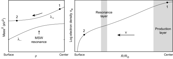
Figure 15: Adiabatic flavor conversion by the MSW mechanism in the Sun. An electron neutrino is produced at Point 1 where the density lies above that of the MSW resonance and propagates radially outward to Point 2 where the density lies below that of the resonance. The width of the resonance layer is assumed to be much larger than the matter oscillation length in the resonance layer, justifying the adiabatic approximation of Eq. (44). Widths of resonance and production layers are not meant to be to scale in this figure.

An electron neutrino is produced at Point 1 near the center of the Sun and propagates radially outward to Point 2. Detection is assumed to average over many oscillation lengths so that the interference terms are washed out and our concern is with the classical (time-averaged) probability, as described in Section III.3. The probability to be detected at Point 2 in the $|\nu_{\mbox{\scriptsize e}}\rangle$ flavor eigenstate is then given by kuo1989

$$\bar{P}(\nu_{\mbox{\scriptsize e}}{\,\scriptstyle\rightarrow\,}\nu_{\mbox{\scriptsize e}}) =(1\ \ \ 0)\begin{pmatrix}\cos^{2}\theta_{\mbox{\scriptsize m}}(2)&\sin^{2}\theta_{\mbox{\scriptsize m}}(2)\\ \sin^{2}\theta_{\mbox{\scriptsize m}}(2)&\cos^{2}\theta_{\mbox{\scriptsize m}}(2\end{pmatrix}$$

$$\times\small\left(\begin{array}[]{cc}1&0\\ 0&1\end{array}\right)\begin{pmatrix}\cos^{2}\theta_{\mbox{\scriptsize m}}(1)&\sin^{2}\theta_{\mbox{\scriptsize m}}(1)\\ \sin^{2}\theta_{\mbox{\scriptsize m}}(1)&\cos^{2}\theta_{\mbox{\scriptsize m}}(1)\end{pmatrix}\begin{pmatrix}1\\ 0\end{pmatrix},$$

where $\theta_{\mbox{\scriptsize m}}(i)\equiv\theta_{\mbox{\scriptsize m}}(t_{i})$ and the row vector $(1\ 0)$ and corresponding column vector denote a pure $\nu_{\mbox{\scriptsize e}}$ flavor state. Evaluating the matrix products and using standard trigonometric identities,

$$\bar{P}(\nu_{\mbox{\scriptsize e}}{\,\scriptstyle\rightarrow\,}\nu_{\mbox{\scriptsize e}})=\tfrac{1}{2}\left[1+\cos 2\theta_{\mbox{\scriptsize m}}(t_{1})\cos 2\theta_{\mbox{\scriptsize m}}(t_{2})\right].$$ (46)

This result is valid (if the adiabatic condition is satisfied) for Point 2 anywhere outside Point 1, but in the specific case that Point 2 lies at the solar surface $\theta_{\mbox{\scriptsize m}}(t_{2})\rightarrow\theta$ and the classical probability to detect the neutrino as an electron neutrino when it exits the Sun is

$$\bar{P}(\nu_{\mbox{\scriptsize e}}{\,\scriptstyle\rightarrow\,}\nu_{\mbox{\scriptsize e}})=\tfrac{1}{2}\left[1+\cos 2\theta\cos 2\theta^{\scriptscriptstyle 0}_{\rm\scriptscriptstyle m}\right],$$ (47)

where $\theta$ is the vacuum mixing angle and $\theta^{\scriptscriptstyle 0}_{\rm\scriptscriptstyle m}\equiv\theta_{\mbox{\scriptsize m}}(t_{1})$ is the matter mixing angle at the point of neutrino production.

IV.9.2 Dependence Only on the Mixing Angle

Equation (47) has a simple physical interpretation. The mass matrix for a neutrino propagating down the solar density gradient is diagonal by virtue of the adiabatic assumption (44), so a neutrino produced in the $\lambda_{+}$ eigenstate remains in that mass eigenstate until it reaches the solar surface, with the flavor conversion resulting only from the change of mixing angle between the production point and the surface. Thus, in adiabatic approximation the classical probability $\bar{P}(\nu_{\mbox{\scriptsize e}}{\,\scriptstyle\rightarrow\,}\nu_{\mbox{\scriptsize e}})$ depends only on the mixing angles at the point of production and point of detection, and is independent of the details of neutrino propagation. This is reminiscent of the results obtained in Section III.3 for the classical average of vacuum oscillations; indeed, Eq. (47) is equivalent to Eq. (12) in the limit that $\theta_{\mbox{\scriptsize m}}\rightarrow\theta$. MSW flavor conversion in adiabatic approximation is illustrated for four different values of the vacuum mixing angle $\theta$ in Fig. 16.

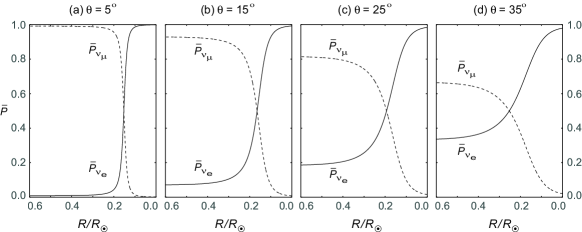
Figure 16: MSW flavor conversion versus fraction of solar radius for four values of the vacuum mixing angle $\theta$ in a 2-flavor model. All calculations are classical averages (Section III.3) over local oscillations in adiabatic approximation using Eq. (47) with $\Delta m^{2}=7.6\times 10^{-5}\mbox{\ eV}^{2}$ and $E=10\mbox{\ MeV}$. The exponential density approximation shown in Fig. 2 was used and neutrinos were assumed to be produced in a $\nu_{\mbox{\scriptsize e}}$ flavor state at the center (right side of diagram at $R/R_{\odot}=0$). Solid curves show the classical electron-neutrino probability $\bar{P}_{\nu_{\scriptscriptstyle\rm e}}\equiv\bar{P}(\nu_{\mbox{\scriptsize e}}{\,\scriptstyle\rightarrow\,}\nu_{\mbox{\scriptsize e}})$ and dashed curves show the corresponding classical muon-neutrino probability $\bar{P}_{\nu_{\mu}}\equiv\bar{P}(\nu_{\mbox{\scriptsize e}}{\,\scriptstyle\rightarrow\,}\nu_{\mu})$. In these figures the MSW resonance occurs at the radius corresponding to the intersection of the solid and dashed curves.

Figure 16(d) approximates the situation expected for the Sun.

IV.9.3 Resonant Conversion for Large or Small $\bm{\theta}$

As shown in Fig. 8(a), the matter mixing angle $\theta_{\mbox{\scriptsize m}}$ approaches $\frac{\pi}{2}$ near the center of the Sun and becomes equal to $\theta$ at the surface of the Sun. Hence neutrinos are produced in a flavor eigenstate that is an almost pure mass eigenstate, but they evolve to a flavor mixture characterized by the vacuum mixing angle $\theta$ by the time they exit the Sun. The most rapid flavor conversion occurs around the MSW resonance where the $P_{\nu_{\scriptscriptstyle\rm e}}$ and $P_{\nu_{\mu}}$ curves intersect. For smaller vacuum mixing angle $\theta$ almost complete flavor conversion occurs in the resonance, while for the large mixing angle case of Fig. 16(d) about $\frac{2}{3}$ of 10-MeV $\nu_{\mbox{\scriptsize e}}$ produced in the core will undergo flavor conversion before leaving the Sun.

IV.9.4 Energy Dependence of Flavor Conversion

Figure 14 suggests that flavor conversion has a significant energy dependence. For example, repeating the calculation of Fig. 16(d) for a range of neutrino energies $E$ gives the electron neutrino survival probabilities displayed in Table 2,

Table 2: Energy dependence of solar neutrino flavor conversion for a vacuum mixing angle $\theta=35^{\circ}$

$E$ (MeV)	14	10	6	2	1	0.70
$P_{\nu_{\scriptscriptstyle\rm e}}$ (surface)	0.33	0.33	0.34	0.40	0.47	0.50
$R^{\rm\scriptscriptstyle R}/R_{\odot}$	0.28	0.25	0.20	0.10	0.03	0.0

along with the fractional solar radius $R^{\rm\scriptscriptstyle R}/R_{\odot}$ where the MSW resonance occurs for that energy. From the spectrum in Fig. 1 and the experimental neutrino anomalies of Table 1, one sees an overall suppression of expected electron neutrino probabilities to the 30%–50% range by the MSW effect, with the lower end of this range associated with higher-energy neutrinos. These results suggest a possible resolution of the solar neutrino problem that will be elaborated further in Section V.

V Resolving the Solar Neutrino Problem

The two-flavor neutrino oscillation formalism described above may now be used in conjunction with a series of key neutrino observations by Super Kamiokande, the Sudbury Neutrino Observatory (SNO), and KamLAND to resolve the solar neutrino problem. As will now be summarized, this analysis indicates that electron neutrinos are being converted to other flavors by neutrino oscillations, that the solar neutrino “deficit” disappears if all flavors of neutrinos coming from the Sun are detected, and that the favored oscillation scenario is MSW resonance conversion in the Sun for a large vacuum mixing angle solution.

V.1 Super Kamiokande Observation of Flavor Oscillation

Cosmic rays striking the atmosphere generate showers of mesons that decay to muons, electrons, positrons, and neutrinos. The Super Kamiokande (Super K) detector in Japan was used to observe neutrinos produced in these atmospheric cosmic ray showers. These measurements found that the ratio of muon neutrinos and antineutrinos to electron neutrinos and antineutrinos was less than $\sim 64\%$ of the value expected from the Standard Model, and the results were interpreted as an indication that the muon neutrino was undergoing oscillations with another flavor neutrino that was not the electron neutrino. fuk98 This was the first conclusive evidence of neutrino oscillations and thus of finite neutrino mass.

V.2 SNO Observation of Neutral Current Interactions

The Super Kamiokande atmospheric neutrino results cited above indicate the existence of neutrino oscillations and thus of physics beyond the Standard Model. The neutrino oscillations discovered by Super Kamiokande are not directly applicable to the solar neutrino problem because they do not appear to involve electron neutrinos. However, a modified water Cherenkov detector operating in Canada has yielded information about neutrino oscillations that does have implications for the solar neutrino problem.

V.2.1 SNO and Heavy Water

The Sudbury Neutrino Observatory (SNO) differed from Super Kamiokande in that it contained heavy water (water enriched in deuterium, ²H) at its core. In regular water solar neutrinos can signal their presence only by elastic scattering from electrons, which typically requires about 5–7 MeV of energy to produce Cherenkov light for reliable detection. However, the deuterium (d) contained in the heavy water can undergo a breakup reaction when struck by a neutrino through the weak neutral current, where any flavor neutrino can initiate the reaction

$$\nu+d\rightarrow\nu+p+n\qquad\mbox{\ (Neutral current) ,}$$ (48)

and the charged weak current reaction

$$\nu_{\mbox{\scriptsize e}}+d\rightarrow e^{-}+p+p\qquad\mbox{\ (Charged current)},$$ (49)

which can be initiated only by electron neutrinos. These reactions have much larger cross sections than elastic neutrino–electron scattering, and the energy threshold can be lowered to 2.2 MeV, the binding energy of the deuteron. Crucially, the neutral-current reaction (48) is flavor blind, which gave SNO the ability to see the total neutrino flux of all flavors coming from the Sun.

V.2.2 Observation of Flavor Conversion for Solar Neutrinos

The SNO results are summarized concisely in Table 3 and Fig. 17(a).

Table 3: Comparison of SNO results and Standard Solar Model (SSM) for solar neutrino fluxes. ahm02a ; ahm02b Fluxes in units of $10^{6}\ {\rm cm}^{2}\,{\rm s}^{-1}.$

SSM $\nu_{\mbox{\scriptsize e}}$ flux	SNO $\nu_{\mbox{\scriptsize e}}$ flux	SNO $\nu_{\mbox{\scriptsize e}}$/SSM	SNO all flavors	SNO all/ SSM
$5.05\pm 0.91$	$1.76\pm 0.11$	0.348	$5.09\pm 0.62$	1.01

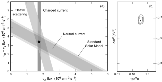
Figure 17: (a) Flux of solar neutrinos from ⁸B detected for various flavors by SNO. ahm02a The band widths represent one standard deviation. Note that the bands intersect at the point indicated by the star, which implies that about $\frac{2}{3}$ of the Sun’s ⁸B neutrinos have changed flavor between being produced in the core of the Sun and being detected on Earth. The Standard Solar Model band is the prediction for the ⁸B flux, irrespective of flavor changes. Note that it tracks the neutral current band, which represents detection of all flavors of neutrino coming from the Sun. (b) 2-flavor neutrino oscillation parameters determined by SNO ahm02b . The 99%, 95% and 90% confidence-level contours are shown, with the star at the most likely value. The best fit corresponds to the large-angle solution given in Eq. (50).

The SNO observations confirmed results from the pioneering solar neutrino experiments summarized in Table 1: a strong suppression of the electron neutrino flux is observed relative to that expected in the Standard Solar Model. ahm02a However, by analyzing the flavor-blind weak neutral current events, the total flux of all neutrinos was found to be almost exactly that expected from the Standard Solar Model. Table 17 summarizes: although the $\nu_{\mbox{\scriptsize e}}$ flux is only 35% of that expected without oscillations, the flux summed over all flavors is 100% of that predicted by the Standard Solar Model for electron neutrino emission, within the experimental uncertainty.

The SNO case was strengthened by analysis of neutrino–electron elastic scattering data combined with data from the charged-current reaction (49). This also allows an estimate of the total neutrino flux of all flavors: in elastic scattering from electrons, both charged and neutral currents contribute for electron neutrinos but only neutral currents do so for other flavors. Figure 17(a) illustrates the flux of neutrinos from the ⁸B reaction, based on SNO results. The best fit indicates that $\frac{2}{3}$ of the Sun’s electron neutrinos have changed flavor by the time they reach Earth.

V.2.3 SNO Flavor-Mixing Solution

Figure 17(b) shows the confidence-level contours for SNO data, which suggest that the solar neutrino problem is solved by $\nu_{\mbox{\scriptsize e}}$–$\nu_{\mu}$ flavor oscillations with

$$\Delta m^{2}=6.5_{-2.3}^{+4.4}\times 10^{-5}\mbox{\ eV}^{2}\qquad\theta=33.9^{+2.4\,^{\circ}}_{-2.2\,^{\circ}}.$$ (50)

This large-mixing-angle solution means that $\nu_{\mbox{\scriptsize e}}$ is almost an equal superposition of two mass eigenstates, separated by at most a few hundredths of an eV.

V.3 KamLAND Constraints on Mixing Angles

KamLAND used phototubes to monitor a large container of liquid scintillator, looking specifically for electron antineutrinos produced during nuclear power generation in a set of nearby Japanese and Korean reactors. Antineutrinos are detected from the inverse $\beta$-decay in the scintillator: $\bar{\nu}_{\mbox{\scriptsize e}}+p\rightarrow e^{+}+n.$ From the power levels in the reactors, the expected antineutrino flux at KamLAND could be modeled accurately. The experiment detected a shortfall of antineutrinos relative to the expected number and this could be accounted for assuming (anti)neutrino oscillations with a large-angle solution having egu03 ; kam2008

$$\Delta m^{2}=7.58^{+0.14}_{-0.13}\times 10^{-5}\mbox{\ eV}^{2}\qquad\tan^{2}\theta=0.56^{+0.10}_{-0.07}$$ (51)

(only statistical uncertainties are indicated), which corresponds to $\theta\sim 36.8^{\circ}$ for the vacuum mixing angle.

The oscillation properties of neutrinos and antineutrinos of the same generation are expected to be equivalent by CPT symmetry, where C is charge conjugation, P is parity, and T is time reversal. Thus the large-angle KamLAND solution for electron antineutrinos may be interpreted as corroboration of the large-angle solution found for solar neutrinos. Combining the solar neutrino and KamLAND results leads to a solution kam2008

$$\Delta m^{2}=7.59\pm 0.21\times 10^{-5}\mbox{\ eV}^{2}\quad\tan^{2}\theta=0.47^{+0.06}_{-0.05},$$ (52)

implying a vacuum mixing angle $\theta\sim 34.4^{\circ}$. The solar neutrino problem is resolved by neutrino oscillations for which the vacuum mixing angle is large (recall that $\theta$ is defined so that its maximum value is $45^{\circ}$).

V.4 Large Mixing Angles and the MSW Mechanism

The large mixing angle solutions found by SNO and KamLAND indicate that the vacuum oscillations of solar neutrinos are of secondary importance to the MSW matter oscillations in the body of the Sun itself in reducing the electron neutrino flux. The large-angle solutions imply vacuum oscillation lengths of a few hundred kilometers, so the classical average (12) applies and for $\theta\sim 34^{\circ}$ the reduction in $\nu_{\mbox{\scriptsize e}}$ flux from averaging over vacuum oscillations is by about $\sim 57\%$. Thus for vacuum oscillations the suppression of the electron neutrino flux detected on Earth would be by a factor of less than two, but the Davis chlorine experiment indicates a suppression by a factor of three. flavor conversion more severe than is possible from vacuum oscillations seems required, and this can be explained by the MSW resonance, as has been illustrated in Fig. 16. Indeed, Fig. 16(d) indicates that for 10 MeV neutrinos and parameters consistent with Eq. (50), the MSW resonance gives a $\nu_{\mbox{\scriptsize e}}$ suppression by a factor of three.

Furthermore, vacuum oscillation lengths for the large-angle solutions are much less than the Earth–Sun distance, which would largely wash out any energy dependence of the electron neutrino shortfall. Since the observations indicate that such an energy dependence exists (see Table 1), and the MSW effect implies such an energy dependence (see Fig. 2 and Table 2), the MSW resonance is implicated as the primary source of the neutrino flavor conversion responsible for the “solar neutrino problem”. That is, the MSW resonance converts from $\frac{1}{2}$ to $\frac{2}{3}$ (depending on the neutrino energy) of electron neutrinos into other flavors within the body of the Sun, and these populations are then only somewhat modified by the vacuum oscillations before the solar neutrinos reach detectors on Earth.

V.5 A Tale of Large and Small Mixing Angles

Initial theoretical prejudice favored a small vacuum mixing angle. The MSW effect attracted initial attention because it was hoped that it might explain how a small mixing angle could account for the solar neutrino deficit, since Fig. 16 indicates that the MSW resonance can generate almost complete flavor conversion even for small vacuum mixing angles. However, data now indicate that the MSW resonance is indeed the solution of the solar neutrino problem, but for a large mixing angle solution. Thus, in this tale an essentially correct physical idea, but with some initially incorrect specific assumptions, led eventually to a surprising resolution of a fundamental problem. As a philosophical aside, this story represents a beautiful example of the scientific method at work.

VI Additional Teaching Resources

The material discussed here is a self-contained introduction to learning and teaching the physics of vacuum and matter solar neutrino oscillations. However, additional resources are available for those who wish to go further. The present paper is a synopsis of a more extensive discussion that may be found in Chapters 10–13 of the book Stars and Stellar Processes (Mike Guidry, Cambridge University Press, 2019). Those chapters contain 25 problems relevant to the present material that go into more technical depth than there is room for here, with complete solutions available online to instructors, and a subset of solutions available online to students, Color lecture slides also are available to instructors from the publisher that are suitable for teaching the present material.

VII Summary

A concise introduction to neutrino vacuum and matter oscillations in a two-flavor model has been presented. Sample calculations with this formalism, in concert with observational data, demonstrate explicitly the resolution of the solar neutrino problem through neutrino flavor oscillations and the associated MSW matter resonance. The intent of this presentation has been to make available to instructors in classes such as astrophysics and quantum mechanics at the advanced undergraduate and beginning graduate level, and to motivated students through self-study, an introduction to the theory of solar neutrino oscillations that assumes only a basic knowledge of quantum mechanics, calculus, differential equations, and $2\times 2$ matrices, and assumes no special prior knowledge of elementary particle physics, quantum field theory, or solar astrophysics.

*

Appendix A Natural Units

The formalism described here uses natural units, chosen such that $\hbar=c=1$. Such units are particularly convenient for relativistic quantum field theories and are ubiquitous in the literature of neutrino oscillations. Conversion between natural units and more standard “engineering units” is basically a dimensional analysis problem. Let’s illustrate with an example. Consider the neutrino oscillation length $L$. Multiply the first expression in Eq. (11) (which is $L$ expressed in $\hbar=c=1$ units) by $c^{4}/c^{4}=1$ to give

$$L=\frac{4\pi Ec^{4}}{\Delta m^{2}c^{4}}=\frac{4\pi Ec^{4}}{\Delta E^{2}},$$

where $\Delta E^{2}\equiv\Delta m^{2}c^{4}$ has units of energy squared. Let $[x]$ denote the units of a variable $x$ and define our standard length unit as ${\cal L}$, our standard energy unit as ${\cal E}$, and our standard time unit as ${\cal T}$. Then dimensionally,

$$[L]=\frac{[E][c^{4}]}{[\Delta E^{2}]}=\frac{{\cal E}{\cal L}^{4}{\cal T}^{-4}}{{\cal E}^{2}}={\cal L}\frac{{\cal L}^{3}}{{\cal E}{\cal T}^{4}}.$$

The final expression should have units of length ${\cal L}$ in normal units, so the preceding result in natural units must be multiplied by a combination of $\hbar$ and $c$ having units of ${\cal E}{\cal T}^{4}/{\cal L}^{3}$ to convert to normal units. Since in normal units

$$[\hbar]={\cal E}{\cal T}\qquad[c]={\cal L}/{\cal T}$$

the required factor is $\hbar/c^{3}$ and

$$L =\frac{\hbar}{c^{3}}\times\frac{4\pi E}{\Delta m^{2}}=\frac{4\pi E\hbar c}{\Delta m^{2}c^{4}}$$

$$=2.48\times 10^{-3}\left(\frac{E}{\mbox{\ MeV}}\right)\left(\frac{\mbox{\ eV}^{2}}{\Delta E^{2}}\right)\mbox{\ km},$$

where the neutrino energy $E$ is in MeV and the energy squared difference $\Delta E^{2}$ corresponding to the mass squared difference $\Delta m^{2}$ is in eV². Transformation between natural units and everyday (engineering) units for other quantities may be carried out in a similar way.

- (1) C. Waltham, “Teaching Neutrino Oscillations,” Am. J. Phys. 72, 742–752 (2004).
- (2) W. C. Haxton and B. R. Holstein, “Neutrino physics,” Am. J. Phys. 68, 15–32 (2000).
- (3) W. C. Haxton and B. R. Holstein, “Neutrino physics: An update,” Am. J. Phys. 72, 18–24 (2004).
- (4) T. K. Kuo and J. Pantaleone, “Neutrino Oscillations in Matter,” Rev. Mod. Phys. 61, 937–979 (1989).
- (5) A. Y. Smirnov, “The msw effect and solar neutrinos,” arXiv: hep-ph/0305106 (2003).
- (6) M. Blennow and A. Y. Smirnov, "Neutrino Propagation in Matter," Advances in High Energy Physics 2013, http://www.hindawi.com/journals/ahep/2013/972485/ (2013).
- (7) J. N. Bahcall, Neutrino Astrophysics, (Cambridge University Press, Cambridge, 1989).
- (8) J. N. Bahcall, M. H. Pinsonneault, and S. Basu, “Solar Models: current epoch and time dependences, neutrinos, and helioseismological properties, ”Astrophys. J. 555, 990 (2001).
- (9) J. N. Bahcall and M. Pinsonneault, “Solar models with helium and heavy-element diffusion,” Rev. Mod. Phys. 67, 781 (1995).
- (10) L. Bonolis, “Bruno Pontecorvo: From slow neutrons to oscillating neutrinos,” Am. J. Phys. 73, 487–499 (2005).
- (11) Particle Data Group at http://pdg.lbl.gov/.
- (12) L. Wolfenstein, “Neutrino oscillations in matter,” Phys. Rev. D17, 2369–2374 (1978).
- (13) S. P. Mikheyev and A. Yu. Smirnov, “Resonant amplification of neutrino oscillations in matter and solar-neutrino spectroscopy,” Nuovo Cimento C9, 17 (1986).
- (14) H. Bethe, “Possible explanation of the solar-neutrino puzzle,” Phys. Rev. Lett. 56, 1305–1308 (1986).
- (15) P. D. B. Collins, A. D. Martin, and E. J. Squires, Particle Physics and Cosmology, (Wiley Interscience, New York, 1989).
- (16) T. Morii, C. S. Lim, and S. N. Mukherjee, The Physics of the Standard Model, (World Scientific, Singapore, 2004).
- (17) W. C. Haxton, “Adiabatic conversion of solar neutrinos,” Phys. Rev. Lett. 57, 1271–1274 (1986).
- (18) G. G. Raffelt, Neutrinos and stars, Proceedings ISAPP School, Varenna, Italy; arXiv: 1201.1637 (2011).
- (19) S. F. King and C. Luhn, “Neutrino Mass and Mixing with Discrete Symmetry”, Rep. Prog. Phys. 76, 056201 (2013).
- (20) Y. Fukuda et al, “Evidence for Oscillation of Atmospheric Neutrinos,” Phys. Rev. Lett. 81, 1562–1567 (1998).
- (21) Q. R. Ahmad et al, “Direct Evidence for Neutrino Flavor Transformation from Neutral-Current Interactions in the Sudbury Neutrino Observatory,” Phys. Rev. Lett. 89, 011301 (2002).
- (22) Q. R. Ahmad et al, “Measurement of Day and Night Neutrino Energy Spectra at SNO and Constraints on Neutrino Mixing Parameters,” Phys. Rev. Lett. 89, 011302 (2002).
- (23) K. Eguchi et al, “First Results from KamLAND: Evidence for Reactor Antineutrino Disappearance,” Phys. Rev. Lett. 90, 021802 (2003).
- (24) S. Abe et al, “Precision Measurement of Neutrino Oscillation Parameters with KamLAND,” Phys. Rev. Lett. 100, 221803 (2008).