Learning from a tiny dataset of manual annotations: a teacher/student approach for surgical phase recognition

Abstract

Purpose

Vision algorithms capable of interpreting scenes from a real-time video stream are necessary for computer-assisted surgery systems to achieve context-aware behavior. In laparoscopic procedures one particular algorithm needed for such systems is the identification of surgical phases, for which the current state of the art is a model based on a CNN-LSTM. A number of previous works using models of this kind have trained them in a fully supervised manner, requiring a fully annotated dataset. Instead, our work confronts the problem of learning surgical phase recognition in scenarios presenting scarce amounts of annotated data (under 25% of all available video recordings).

Methods

We propose a teacher/student type of approach, where a strong predictor called the teacher, trained beforehand on a small dataset of ground truth-annotated videos, generates synthetic annotations for a larger dataset, which another model - the student - learns from. In our case, the teacher features a novel CNN-biLSTM-CRF architecture, designed for offline inference only. The student, on the other hand, is a CNN-LSTM capable of making real-time predictions.

Results

Results for various amounts of manually annotated videos demonstrate the superiority of the new CNN-biLSTM-CRF predictor as well as improved performance from the CNN-LSTM trained using synthetic labels generated for unannotated videos.

Conclusion

For both offline and online surgical phase recognition with very few annotated recordings available, this new teacher/student strategy provides a valuable performance improvement by efficiently leveraging the unannotated data.

1 Introduction

Problem statement

Laparoscopic surgery is, by nature, an abundant source of video data, which deep learning algorithms can leverage for surgical workflow analysis. One particular application that has been examined is phase recognition in surgical procedures. This task is essential for enabling context-aware behavior in Computer-Assisted Surgery: a system capable of identifying surgical phases in real time could use this information to deliver adequate notifications or warnings to a surgeon in the middle of an intervention. Real-time operation is highly desirable in this context: offline predictors may be employed as post-processing tools dedicated to recordings, for educational or archival purposes; but online predictors can directly tap into a live video stream of the procedure and be incorporated into a computer-assisted surgery system. Producing annotations to train such predictors, however, is a potentially tedious process that often requires the presence of clinical experts. This issue creates a strong incentive for exploring semi-supervised methods, specifically tailored for situations in which manual annotations are only provided for a fraction of all available data.

Contribution

For the work presented in this paper, we direct our attention towards surgical phase recognition in scenarios of extreme manual annotation scarcity: 20 manually annotated recordings or fewer, which is 25% or less of the training set’s initial size in our dataset of cholecystectomy recordings. In order to perform phase recognition under these conditions, we propose a teacher/student approach, where the teacher - a model trained on a small set of manually annotated videos - generates synthetic annotations for a large number of videos, which, in turn, serve as training material for another model called the student. In the context of surgical phase recognition, this is, to the best of our knowledge, the first work in which synthetic labels are employed. The teacher model presents a novel architecture that combines a Convolutional Neural Network (CNN), a bidirectional Long-Short-Term-Memory Network (biLSTM) and a Linear-Chain Conditional Random Field (CRF); the student model is a CNN-LSTM. The two models are highly complementary, with on the one hand a teacher exhibiting stronger predictive power but no real-time inference capabilities, and on the other hand a weaker model capable of performing in real time.

Experiments are performed on cholec120, a dataset of 120 cholecystectomy videos rsdnet . Each video frame belongs to one of the 7 following phases: (P1) preparation, (P2) calot triangle dissection, (P3) clipping and cutting, (P4) gallbladder dissection, (P5) gallbladder packaging, (P6) cleaning and coagulation, (P7) gallbladder extraction. When only few ground truth annotated videos are available (e.g. 20), results show improvement for both the CNN-biLSTM-CRF model (75.8% F1 score) trained only on ground truth annotated videos and for the CNN-LSTM trained with synthetic labels (73.2% F1 score), as compared to the CNN-LSTM trained on ground truth annotated videos alone (70.2% F1 score); this brings the performance closer to the CNN-LSTM trained on all 80 manually annotated videos (78.2% F1 score).

Related work

Surgical phase recognition from video data has recently received much attention from the Computer-Assisted Interventions community, and the state-of-the-art approaches rely on deep learning. An example of early work relying on deep learning is Twinanda et. al endonet , which features a combination of CNN and HMM. A staple approach for surgical phase recognition in the fully supervised case combines a CNN, used as a visual feature extractor, with a unidirectional LSTM to model temporal dependencies in the video. This approach was presented in andrum2cai and the related PhD thesis andruphd . The author also experimented with a biLSTM, which showed increased performance but only functioned as an offline predictor. Jin et al. used the same type of model in jin , but aggregated features extracted by the CNN from three timesteps close to each other before feeding the LSTM. The same author later introduced an extension in svrcnet , using Prior Knowledge Inference to post-process the predictions. In our work, we rely on a CNN-LSTM architecture for the student model as well, and a CNN-biLSTM for a large part of the teacher model.

Conditional Random Fields (CRF) have been featured in several works on surgical phase recognition: quellec_crf and charriere_crf both used them for cataract surgery videos. Lea et al. relied on CRFs for analyzing surgical training tasks in lea_crf_1 and lea_crf_2 . None of these approaches, however, have combined them with CNN-extracted visual features or deep recurrent temporal models. The combination of bidirectional LSTM and CRF has been explored by lample_ner and huang_ner in the context of Named Entity Recognition - a problem involving no video data - where the objective is to identify the type of each word in a sentence - for instance object or location. We make use of a biLSTM-CRF combination in our work, in order to obtain well-structured sequences of predictions from the teacher.

data_distillation proposes a teacher/student approach on different target tasks , namely human pose estimation and object detection. These tasks exploit single frames, and do not involve any temporal data. The method relies on synthetic labels generated by ensembling predictions over geometric transforms of the same input image.

A few recent papers have approached surgical phase recognition from the semi-supervised angle, using the same type of CNN-LSTM architecture as in andruphd , but with different training strategies that exploit unannotated videos. The core idea is to pretrain the CNN on a proxy task for which no manual labels are required, in order to encourage it to learn temporally relevant features. bodenstedt used a CNN pretrained on frame sorting. funke trained the CNN to make predictions related to the temporal distance between multiple frames of a video. Experiments were performed on the cholec80 dataset with a full training set size of 60 and mini-training sets of 40 or fewer annotated videos. Similarly, endon2n used the prediction of Remaining Surgery Duration (RSD) as a proxy task, along with end-to-end training of the CNN-LSTM final model. This scheme can be challenging to implement due to the interplay between weight regularization and the range of the model’s output, in addition to the taxing computational requirements of end-to-end training. The corresponding experiments used the cholec120 dataset with a full training set size of 80 and mini-training sets of 64 or fewer annotated videos.

2 Methods

2.1 Overview

The approach presented in this paper relies on a teacher/student dynamic between the two temporal models depicted in Fig.1. The teacher model is trained on a small set of manually annotated videos and generates synthetic labels for every video for which ground truth annotations are unavailable. The pool of synthetically annotated videos and manually annotated videos is then employed to train another model, namely the student. The teacher, in our case, uses a new combination of CNN, biLSTM and CRF to achieve offline inference results superior to what a conventional CNN-LSTM would be capable of, thanks to its ability to take into account information from future timesteps (biLSTM), as well as knowledge on transitions between phases in surgical videos (CRF). The student is a traditional CNN-LSTM, which comes with the major benefit of online inference.

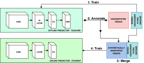
Figure 1: Teacher-student approach overview

2.2 Teacher model

We describe below each component of the CNN-biLSTM-CRF teacher model.

2.2.1 CNN

The chosen CNN architecture is Resnet-50 V2, as introduced by He et al.resnet . It serves as a visual feature extractor, mapping the $256\times 256\times 3$ input RGB images to vector representations of size $N_{f}=2048$. These feature vectors will then serve as input for the temporal model described next.

2.2.2 Bidirectional LSTM

Formally, a unidirectional LSTM maps a sequence of input vectors $(i_{0},...,i_{T})$ to a sequence of output vectors $(o_{0},...,o_{T})$ obeying

$$\forall t\in\llbracket 1,T\rrbracket,(o_{t},c_{t},h_{t})=q_{f}(i_{t},c_{t-1},h_{t-1}),$$ (1)

where $(c_{t}),(h_{t})$ are sequences of states, with $c_{0},h_{0}$ randomly initialized in our case. The function $q_{f}$ as detailed in hochreiter_lstm is the LSTM cell; upon training, $q_{f}$ learns to model temporal dependencies from past timesteps to the current one. graves_bilstm suggests incorporating another LSTM cell, in order to model for temporal dependencies from future samples to the current one. This means introducing another sequence of outputs $(\omega_{0},...,\omega_{T})$ and an LSTM cell $q_{b}$ such that

$$\forall t\in\llbracket 0,T-1\rrbracket,(\omega_{t},\gamma_{t},\eta_{t})=q_{b}(i_{t},\gamma_{t+1},\eta_{t+1}),$$ (2)

again with $(\gamma_{t}),(\eta_{t})$ as sequences of states, with initial values $(\gamma_{T}),(\eta_{T})$. The concatenated pair $(o_{t},\omega_{t})$ therefore contains temporal information from both past and future events. This type of model, while very potent for offline inference, is by nature unsuitable for real-time operation.

2.2.3 Linear-Chain Conditional Random Field (CRF)

A single fully connected layer turns the outputs of the biLSTM into logits of size $N_{c}=7$, one for each surgical phase in a cholecystectomy. In general classification problems, each vector of logits is processed independently from the others, by passing it through the softmax function and computing its cross-entropy against a one-hot encoded label vector during training, and by taking the argmax during inference.

A better approach for our application, where consecutive predictions should be consistent with one another, is to process the entire sequence of logits corresponding to a given video together using a linear-chain conditional random field model (CRF). This can be interpreted as a form of smoothing, done in a more principled manner than in ad-hoc postprocessing methods such as the one featured in jin .

Given a sequence of logits $S=(s_{0},...,s_{T})$, for any given timestep $t$ and class index $k$ we note the $k^{th}$ entry of $s_{t}$ as $s_{t}[k]$. Let $\Theta$ be an $N_{c}\times N_{c}$ real-valued matrix, with entries noted as $\Theta[i,j]$ for class indices $i,j$. The score of any sequence of tags (i.e. predicted classes) $Y=(y_{0},...,y_{T})$ can then be defined as:

$$C(S,Y,\Theta)=\sum_{t=0}^{T}s_{t}[y_{t}]+\sum_{t=0}^{T-1}\Theta[y_{t},y_{t+1}].$$ (3)

The trainable parameter of the model is $\Theta$, called the transition matrix. Using the definition of the score $C$, we are able to define the likelihood of a tag sequence as:

$$p(Y|S)=\frac{e^{C(S,Y,\Theta)}}{\sum\limits_{U\in\llbracket 1,N_{c}\rrbracket^{T+1}}e^{C(S,U,\Theta)}},$$ (4)

which is the entry corresponding to $Y$ in the softmax over all possible tag sequences $U$. We then employ $L=-log(p(Y_{true}|S))$ as our training loss, $Y_{true}$ being the ground truth tag sequence. During inference, the highest scoring tag sequence $Y_{opt}$ is obtained by Viterbi decoding.

2.3 Student model

The student model follows the architecture first established in endonet . It relies on the same Resnet-50 CNN as the teacher model for feature extraction, followed by a unidirectional LSTM. This model is adequate for real-time predictions, since at any given timestep the output only depends on the current input, the previous state and the previous output of the LSTM.

2.4 Training

The dataset we use for all of our experiments, cholec120, contains 120 recordings of laparoscopic cholecystectomy, with an average duration of 38 minutes rsdnet . We reserve 30 for testing and 10 for validation, leaving $N=80$ videos to choose from for training. In the following lines we will refer to:

$$E=\left\{(V_{0},\mathcal{A}(V_{0})),(V_{1},\mathcal{A}(V_{1})),...,(V_{N-1},\mathcal{A}(V_{N-1}))\right\},$$ (5)

as the 80 manually annotated videos to choose from, $V_{k}$ and $\mathcal{A}(V_{k})$ being a video and its ground truth annotations respectively.

Considering the voluntarily low number of annotated videos selected for training (from 20 down to 1), we sample 3 non-overlapping mini-training sets of every size in order to prevent biased results coming from the selection process, and ran our series of experiments independently for each mini-training set. In an effort to match the original training set in terms of featured video lengths, we divide the 80 videos into duration quartiles $Q1$ to $Q4$, then randomly sample videos from $Q1$, $Q2\bigcup Q3$, and $Q4$ with a 20/60/20 ratio respectively. For mini-training sets of only one video the single choice is limited to $Q2\bigcup Q3$ in order to avoid outliers. The mini-training sets are referred to as:

$$E_{i,j}=\left\{(V_{k},\mathcal{A}(V_{k})),...\right\},$$ (6)

where $i\in\{1,3,5,10,20\}$ indicates the size of the set of ground truth labeled videos employed, and $j\in\{0,1,2\}$ is the index for the first, second or third experiment for that particular size.

In all of the following experiments, the Resnet-50 CNN is initialized with ImageNet pretrained weights. Test accuracy on ImageNet for those weights reaches 75.6%. The teacher model’s CNN is first pretrained with only one fully connected layer on top, on $E_{i,j}$, directly for phase recognition. Weights from the first and second blocks of Resnet are frozen. Data augmentation is applied using $\pm 16^{\circ}$ rotations and 4 different translations. Visual feature vectors are then extracted from $E_{i,j}$ using the pretrained CNN.

The biLSTM - CRF is then trained end-to-end on the extracted features with untruncated backpropagation through time across the entire video, with the loss function defined in section 2.2.3 similarly to lample_ner and huang_ner .

Using the trained biLSTM - CRF, we generate new annotations for videos in $E\backslash E_{i,j}$. This leads to the set of videos with synthetic annotations:

$$F_{i,j}=\left\{(V_{k},\widehat{\mathcal{A}_{i,j}}(V_{k})),...\right\}.$$ (7)

We then define $G_{i,j}=E_{i,j}\bigcup F_{i,j}$, which contains all videos from the original training set, and combines a small set of manual annotations with a majority of synthetic labels. The student CNN-LSTM model is trained in the same two-step manner, this time on $G_{i,j}$.

Hyperparameters used for training are detailed in table 1. All experiments are performed using Tensorflow with the Adam optimizeradam , on servers fitted with Nvidia 1080Ti GPUs.

Table 1: Table detailing hyperparameters for the featured experiments

CNN pretraining
Learning rate	$5\cdot 10^{-5}$
# of epochs	27
Minibatch size	32
Weight decay	$5\cdot 10^{-4}$
LSTM
Learning rate	$5\cdot 10^{-5}$
# of epochs	350
State size	128
Dropout	0.3
Weight decay	$5\cdot 10^{-4}$

CRF
Learning rate	$5\cdot 10^{-5}$
# of epochs	350
Weight decay	$5\cdot 10^{-3}$
BiLSTM/BiLSTM-CRF
Learning rate (biLSTM)	$1\cdot 10^{-3}$
Learning rate (biLSTM-CRF)	$1\cdot 10^{-4}$
# of epochs	350
State size	$2\cdot 64$
Dropout	0.4
Weight decay	$5\cdot 10^{-4}$

2.5 Complementary studies

2.5.1 Ablation studies

In order to demonstrate the need for every component in the teacher model, we conduct a series of ablation studies by training and evaluating the following models: (M1) CNN (obtained from the pretraining step), (M2) CNN-CRF, (M3) CNN-unidirectional LSTM, (M4) CNN-biLSTM

Temporal models M2 to M4 are trained in the same two-step manner as the proposed CNN-biLSTM-CRF model, referred to as M5.

2.5.2 Full supervision

In order to provide comparison points with the fully supervised approach, the teacher model along with every model featured in the ablation studies are also trained on the original set of 80 manually annotated videos.

2.5.3 Self-learning of the teacher model

The only student model mentioned so far is the CNN-unidirectional LSTM, due to its real-time inference capabilities. Another interesting possibility is to also use a CNN-biLSTM-CRF as the student, in order to obtain a stronger offline predictor.

3 Results & discussion

To demonstrate the benefits of our approach, we have conducted a total number of 125 experiments, counting all mini-training set sizes and all the models featured in the complementary studies. To test our models, we reported their accuracy, precision, recall and F1 score during inference on the test set. Unless otherwise specified, precision, recall and F1 are averaged over the 7 classes. For every metric at a given mini-training set size, we provide the mean and standard deviation over the 3 repeats of the corresponding experiment.

3.1 Teacher model performance

Results for every mini-training set size, the proposed teacher model (M5) and models from the ablation study (M1 to M4) are shown in table 2. Directly applying the CRF after the CNN (M2) yields poor results, likely due to temporal noise affecting the logits emitted by the CNN. Temporal models trained on a single video are severely affected by overfitting, and therefore also exhibit subpar performance. With 3 or more manually annotated videos, however, the biLSTM and the CRF deliver significant performance improvements.

Table 2: Ablation study for the teacher model, accuracy and average F1

		1	3	5	10	20	80
M1	Acc	$40.8\pm 2.6$	$57.3\pm 1.5$	$62.2\pm 1.2$	$67.4\pm 1.5$	$71\pm 1.9$	$75.3$
	F1	$23\pm 4.3$	$39.9\pm 4.1$	$48.8\pm 2.6$	$56\pm 1.9$	$59.1\pm 1.6$	$63.8$
M2	Acc	$41\pm 3.5$	$58\pm 1.2$	$63\pm 0.6$	$65\pm 0.3$	$72.5\pm 1.9$	$80.5$
	F1	$22.1\pm 5.2$	$40.7\pm 4.6$	$48.5\pm 3.3$	$54.3\pm 1.3$	$59.9\pm 1.8$	$69.7$
M3	Acc	$40.1\pm 4.7$	$65.4\pm 5.7$	$72.3\pm 0.9$	$74.7\pm 2.6$	$80.5\pm 0.7$	$86.3$
	F1	$5\pm 2.9$	$47.4\pm 9.9$	$57.9\pm 1.8$	$62.7\pm 3$	$70.2\pm 1.3$	$78.2$
M4	Acc	$36.5\pm 4.7$	$66.3\pm 3.7$	$73.7\pm 1.6$	$76.6\pm 3$	$82.6\pm 0.6$	$88.4$
	F1	$2.9\pm 3$	$47.9\pm 8.5$	$60.1\pm 5$	$67\pm 3.8$	$74.5\pm 1.3$	$81.7$
M5	Acc	$40.1\pm 3.1$	$71.1\pm 4.6$	$76.2\pm 0.3$	$78.5\pm 2.6$	$84.1\pm 1$	$89.5$
	F1	$21.1\pm 11$	$55.3\pm 9$	$65.8\pm 1.2$	$69.7\pm 1.3$	$75.8\pm 1.5$	$82.5$

The CNN-biLSTM (M4) achieves stronger performance than the CNN-unidirectional LSTM (M2), although not as much as the full CNN-biLSTM-CRF model (M5), which is consistently the best performer (Fig. 2). This is observed on all mini-training set sizes except for single videos. As expected, increasing the number of videos improves all global metrics - accuracy, average F1, average precision, average recall - although per-phase precision and recall may fluctuate (table 3). This establishes the CNN-biLSTM-CRF model as the strongest predictor, and therefore the best suited for the role of teacher.

Figure 2: Ablation study models performance as a function of the number of manually annotated videos employed

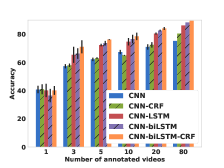
(a) Accuracy

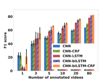
(b) F1 score

Table 3: Per-phase precision and recall, CNN-biLSTM-CRF model

		1	3	5	10	20	80
P1	Pre	$5.5\pm 8.4$	$59.6\pm 0.8$	$52\pm 14.3$	$56.9\pm 14.7$	$68.4\pm 8.3$	$86.6$
	Rec	$56.6\pm 26.7$	$77.4\pm 14.8$	$51.7\pm 4.8$	$54.4\pm 14.1$	$92.6\pm 4.5$	$96.4$
P2	Pre	$48.3\pm 42.3$	$48.1\pm 10.5$	$80.1\pm 3.7$	$77.1\pm 0.9$	$58.8\pm 10$	$68.9$
	Rec	$24.8\pm 23.7$	$83.5\pm 10.7$	$84.7\pm 3.1$	$90.6\pm 5$	$87.2\pm 2.2$	$83.4$
P3	Pre	$36.7\pm 25$	$76.9\pm 12.6$	$62.6\pm 17$	$80.4\pm 11.5$	$93.4\pm 3.9$	$96.5$
	Rec	$50.5\pm 44.9$	$64.3\pm 15.8$	$39.4\pm 26.1$	$31.6\pm 10.9$	$75.9\pm 2.9$	$79.9$
P4	Pre	$61.3\pm 10.4$	$75.4\pm 3.2$	$81.1\pm 5.2$	$86.3\pm 6.7$	$83.1\pm 3.3$	$89.4$
	Rec	$45.9\pm 45.2$	$50.1\pm 29$	$84.4\pm 4.8$	$80.4\pm 1.8$	$70.3\pm 8.8$	$72.7$
P5	Pre	$0\pm 0$	$10.9\pm 15.5$	$74.4\pm 3.1$	$77.7\pm 0.8$	$42.6\pm 5.1$	$53.5$
	Rec	$12.9\pm 11.6$	$71.8\pm 16.2$	$83.3\pm 1.7$	$84\pm 3.1$	$83.2\pm 1.4$	$88.2$
P6	Pre	$3.7\pm 6.4$	$38.7\pm 29.5$	$80.4\pm 2.1$	$76.2\pm 4.2$	$85.1\pm 2.8$	$91.5$
	Rec	$11.3\pm 16.6$	$71\pm 11.9$	$46.7\pm 7.6$	$61.5\pm 5.4$	$81.2\pm 3.6$	$91.5$
P7	Pre	$60.3\pm 44.7$	$82.1\pm 8.5$	$64.1\pm 7.9$	$70.8\pm 1.6$	$87.1\pm 3.6$	$94.1$
	Rec	$50.3\pm 38.9$	$64.6\pm 8.3$	$77.7\pm 10.1$	$77.8\pm 9.5$	$80\pm 4.1$	$77.3$
Avg	Pre	$26.4\pm 4.5$	$62\pm 6.1$	$70.4\pm 4.2$	$75.1\pm 1.6$	$75.8\pm 1.4$	$82.6$
	Rec	$40.5\pm 18.5$	$62.9\pm 7.5$	$66.8\pm 4.7$	$68.6\pm 0.5$	$79.8\pm 1.3$	$84.5$

To qualitatively appreciate improvements from the new model, the predictions on six videos from the test set are presented in Fig.3: the top three and bottom three of the CNN-biLSTM-CRF ranked by accuracy. The CNN-biLSTM-CRF makes the most sensible predictions with respect to the chronological order between the phases; it more specifically avoids inferring incorrect phases in short isolated bursts as the biLSTM sometimes does.

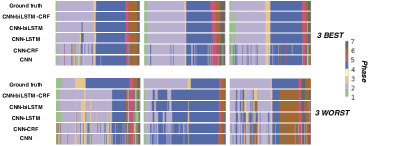
Figure 3: Top 3 best and top 3 worst examples of predictions by time on full videos, from models trained on 20 videos

Table 4: Teacher-completed annotation set metrics

		1	3	5	10	20
P1	Pre	$44.4\pm 33.4$	$63.5\pm 10.5$	$68.8\pm 10.3$	$78.2\pm 5.3$	$85.9\pm 5.5$
	Rec	$4.6\pm 5$	$55.2\pm 3.4$	$47.9\pm 2.8$	$52.4\pm 12.7$	$73.5\pm 4.3$
P2	Pre	$60.9\pm 4.7$	$81.1\pm 1.9$	$86\pm 2.5$	$83.1\pm 2.3$	$90.3\pm 1.6$
	Rec	$35.4\pm 17.2$	$77.4\pm 5.7$	$79.1\pm 6.6$	$88.9\pm 0.3$	$91.6\pm 3$
P3	Pre	$79.7\pm 28.8$	$67.9\pm 9.4$	$66.2\pm 18.7$	$76.3\pm 5.4$	$84.3\pm 2.5$
	Rec	$0.6\pm 0.2$	$19.5\pm 12.3$	$47\pm 23.2$	$40.9\pm 7$	$60\pm 5.8$
P4	Pre	$53.6\pm 18.6$	$72.7\pm 10.5$	$74.5\pm 4$	$83.2\pm 0.6$	$87.4\pm 3.6$
	Rec	$60.8\pm 36.9$	$84.6\pm 5.2$	$89.2\pm 2.9$	$86.4\pm 4.4$	$92.5\pm 1.5$
P5	Pre	$87.2\pm 11.4$	$66.6\pm 14.9$	$77.6\pm 1.9$	$82.8\pm 3.1$	$83.9\pm 2.9$
	Rec	$23.2\pm 16.5$	$78.6\pm 9.1$	$81.7\pm 1$	$81.1\pm 4.2$	$88.3\pm 2.1$
P6	Pre	$43.4\pm 39.5$	$70.1\pm 9.1$	$71.8\pm 7.5$	$76.9\pm 4.2$	$87.3\pm 1.2$
	Rec	$43.9\pm 38.9$	$52.2\pm 24.1$	$51.2\pm 10.1$	$71.2\pm 10.1$	$82\pm 4$
P7	Pre	$58.1\pm 31.3$	$62.4\pm 5$	$63.3\pm 9.2$	$71.8\pm 5.9$	$84.4\pm 4.3$
	Rec	$13.4\pm 14.8$	$72.3\pm 8.1$	$77.6\pm 7.9$	$81.2\pm 1.8$	$84.2\pm 2.6$
Avg	Pre	$61.3\pm 3.8$	$69.2\pm 2$	$72.6\pm 5.3$	$78.9\pm 0.8$	$86.2\pm 1.3$
	Rec	$26\pm 15.7$	$62.8\pm 5.3$	$67.7\pm 4.7$	$71.7\pm 2.3$	$81.7\pm 0.6$
Acc		39.2 $\pm$ 4.7	73.1 $\pm$ 3.1	76.6 $\pm$ 1.2	81.6 $\pm$ 1	88 $\pm$ 1.2
F1		23.5 $\pm$ 3.2	62 $\pm$ 4.7	67.6 $\pm$ 0.8	73.7 $\pm$ 2.1	83.5 $\pm$ 1.1

3.2 Quality of the teacher-completed annotation sets

In order to confirm the quality of the material the student model learns from, we ran our metrics on the annotations from $G_{i,j}$, which mix ground truth annotations and teacher-generated annotations. Results are shown in Table 4. As expected, teachers trained on more manually annotated videos produce better annotations. The presence of more manually annotated videos in the $G_{i,j}$ sets also contributes to greater overall label quality, e.g. 83.5 % F1 score for $G_{20,j}$ on average. Per-phase results indicate stronger performance on phases P2 (90.3% precision, 91.6 % recall for 20 manually annotated videos) and P4 (87.4% precision, 92.5 % recall), which are usually the most prevalent. Despite uneven results across phases, $G_{i,j}$ sets obtained from 3 or more manually annotated videos appear to be overall serviceable for training a student model.

3.3 Student model performance

To appreciate the benefits of using our synthetic labels, we compare in the first two groups of rows of Table 5 the CNN-LSTM only trained with few manually annotated videos against the CNN-LSTM trained with these same videos and annotations plus the videos annotated by the teacher. Results for a single ground truth-annotated video, as one can expect from the results of the corresponding teacher models, are quite poor. Even though the $G_{1,j}$ sets contain 80 times as many videos as the $E_{1,j}$ used for the teachers, the quality of the annotations, as shown in section 3.2, is extremely low. CNN-LSTM models trained on those all exhibit sub-50% performance on every global metric, despite showing some improvement compared to the CNN-LSTM trained on $E_{1,j}$. Decent results are observed starting from 3 videos, with a 2.9 to 8.8 point increase in accuracy when adding synthetic annotations, and similar increase in F1 score.

With 80 ground truth-annotated videos, accuracy and F1 reach 86.3% and 78.2% respectively (Table 5). Therefore, the use of synthetic annotations roughly reduces the performance gap between using 20 and 80 ground truth-annotated videos by half.

Table 5: Performance with and without teacher-generated annotations.

		1	3	5	10	20
CNN-LSTM, no teacher	Acc	$40.1\pm 4.7$	$65.4\pm 5.7$	$72.3\pm 0.9$	$74.7\pm 2.6$	$80.5\pm 0.7$
	Pre	$20.7\pm 1.9$	$51.7\pm 7.1$	$60.4\pm 2.9$	$64.1\pm 1.5$	$71.1\pm 0.7$
	Rec	$17.5\pm 7.5$	$58.6\pm 8.2$	$64\pm 5.5$	$68\pm 3.1$	$64.1\pm 2.7$
	F1	$5\pm 2.9$	$47.4\pm 9.9$	$57.9\pm 1.8$	$62.7\pm 3$	$70.2\pm 1.3$
CNN-LSTM, with teacher	Acc	$42.1\pm 6.3$	$74.6\pm 3.6$	$77.7\pm 0.8$	$79.1\pm 0.9$	$83.4\pm 0.3$
	Pre	$24.6\pm 5.6$	$63\pm 5$	$65.8\pm 5.1$	$66.6\pm 1.7$	$73.5\pm 1.2$
	Rec	$38.9\pm 19.4$	$65.1\pm 7.3$	$72.3\pm 5.2$	$74.7\pm 1.7$	$76.8\pm 0.7$
	F1	$14.5\pm 13.5$	$56.1\pm 8.6$	$64.5\pm 2.9$	$66.9\pm 3.1$	$73.2\pm 0.8$
CNN-biLSTM-CRF, no teacher	Acc	$40.1\pm 3.1$	$71.1\pm 4.6$	$76.2\pm 0.3$	$78.5\pm 2.6$	$84.1\pm 1$
	Pre	$26.4\pm 4.5$	$62\pm 6.1$	$70.4\pm 4.2$	$75.1\pm 1.6$	$75.8\pm 1.4$
	Rec	$40.5\pm 18.5$	$62.9\pm 7.5$	$66.8\pm 4.7$	$68.6\pm 0.5$	$79.8\pm 1.3$
	F1	$21.1\pm 11$	$55.3\pm 9$	$65.8\pm 1.2$	$69.7\pm 1.3$	$75.8\pm 1.5$
CNN-biLSTM-CRF, with teacher	Acc	$43.1\pm 7.5$	$74.9\pm 4.6$	$78.7\pm 1$	$80.8\pm 0.8$	$86.3\pm 1$
	Pre	$26.3\pm 4.1$	$64.2\pm 5.8$	$67.4\pm 5.9$	$70.2\pm 2.7$	$78\pm 1.4$
	Rec	$38.8\pm 16.5$	$65\pm 7.3$	$73.8\pm 5$	$76.9\pm 1.9$	$81.7\pm 0.5$
	F1	$18.2\pm 10.9$	$55.7\pm 9.7$	$66.8\pm 2.7$	$69.9\pm 4$	$78.1\pm 1$

3.4 Self-learning of the teacher model

By using the $G_{i,j}$ sets to train a new CNN-biLSTM-CRF model, the offline performance increases even further (Table 5, last 2 groups of rows) - except for the 1-video case, where performance actually degrades. Results with 20 ground truth-annotated videos are particularly notable, as they match those obtained with 80 ground truth-annotated videos from the CNN-LSTM model (86.3% accuracy, 78.2% F1).

4 Conclusion

The work presented in this paper shows the superior performance of the new CNN-biLSTM-CRF teacher architecture compared to the previous CNN-LSTM used for surgical phase recognition. Although this model is restricted to offline inference, we also propose a teacher/student strategy that leverages the new model for real-time prediction, by exploiting it as a source of synthetic annotations for a CNN-LSTM student model.

Experimental results, obtained using manual annotations for 25% or less of all available training data, show serious potential for scaling surgical phase recognition to a large number of videos while alleviating the burden of collecting manual annotations. The performance deficit between scenarios with 25% and 100% ground truth annotation availability is halved for a CNN-LSTM online prediction model when adding synthetic labels from the teacher. When swapping the student for a CNN-biLSTM-CRF offline prediction model, the gap is fully closed. Many other types of surgical procedures than cholecystectomy, for which large amounts of annotated data are not yet available, might be able to benefit from this method as well.

• Conflicts of interest The authors declare that they have no conflict of interest.
  Ethical approval This article does not contain any studies with human participants or animals performed by any of the authors.
  Informed consent Statement of informed consent was not applicable since the manuscript does not contain any patient data.

References

- (1) Bodenstedt, S., Wagner, M., Katic, D., Mietkowski, P., Mayer, B.F.B., Kenngott, H., Müller-Stich, B.P., Dillmann, R., Speidel, S.: Unsupervised temporal context learning using convolutional neural networks for laparoscopic workflow analysis (2017)
- (2) Charrière, K., Quellec, G., Lamard, M., Martiano, D., Cazuguel, G., Coatrieux, G., Cochener, B.: Real-time analysis of cataract surgery videos using statistical models. Multimedia Tools Appl. 76(21), 22473–22491 (2017)
- (3) Funke, I., Jenke, A., Mees, S.T., Weitz, J., Speidel, S., Bodenstedt, S.: Temporal coherence-based self-supervised learning for laparoscopic workflow analysis. In: OR 2.0 Context-Aware Operating Theaters, Computer Assisted Robotic Endoscopy, Clinical Image-Based Procedures, pp. 85–93 (2018)
- (4) Graves, A., Schmidhuber, J.: Framewise phoneme classification with bidirectional lstm and other neural network architectures 18, 602–10 (2005)
- (5) He, K., Zhang, X., Ren, S., Sun, J.: Identity mappings in deep residual networks. In: Computer Vision - ECCV - 14th European Conference Part IV, pp. 630–645 (2016)
- (6) Hochreiter, S., Schmidhuber, J.: Long short-term memory 9, 1735–80 (1997)
- (7) Huang, Z., Xu, W., Yu, K.: Bidirectional LSTM-CRF models for sequence tagging (2015)
- (8) Jin, Y., Dou, Q., Chen, H., Yu, L., Heng, P.A.: Endorcn: recurrent convolutional networks for recognition of surgical workflow in cholecystectomy procedure video. Tech. rep., The Chinese University of Hong Kong (2016)
- (9) Jin, Y., Dou, Q., Chen, H., Yu, L., Qin, J., Fu, C.W., Heng, P.A.: Sv-rcnet: Workflow recognition from surgical videos using recurrent convolutional network. IEEE transactions on medical imaging 37(5), 1114–1126 (2018)
- (10) Kingma, D.P., Ba, J.: Adam: A method for stochastic optimization (2014)
- (11) Lample, G., Ballesteros, M., Subramanian, S., Kawakami, K., Dyer, C.: Neural architectures for named entity recognition. In: Conference of the North American Chapter of the Association for Computational Linguistics: Human Language Technologies, pp. 260–270 (2016)
- (12) Lea, C., Hager, G.D., Vidal, R.: An improved model for segmentation and recognition of fine-grained activities with application to surgical training tasks. In: 2015 IEEE Winter Conference on Applications of Computer Vision, pp. 1123–1129 (2015)
- (13) Lea, C., Vidal, R., Hager, G.D.: Learning convolutional action primitives for fine-grained action recognition. 2016 IEEE International Conference on Robotics and Automation pp. 1642–1649 (2016)
- (14) Quellec, G., Lamard, M., Cochener, B., Cazuguel, G.: Real-time segmentation and recognition of surgical tasks in cataract surgery videos. IEEE transactions on medical imaging 33(12), 2352–2360 (2014)
- (15) Radosavovic, I., Dollár, P., Girshick, R., Gkioxari, G., He, K.: Data distillation: Towards omni-supervised learning. In: Proceedings of the IEEE Conference on Computer Vision and Pattern Recognition, pp. 4119–4128 (2018)
- (16) Twinanda, A.P.: Vision-based approaches for surgical activity recognition using laparoscopic and RBGD videos. Theses, Université de Strasbourg (2017)
- (17) Twinanda, A.P., Mutter, D., Marescaux, J., de Mathelin, M., Padoy, N.: Single- and multi-task architectures for tool presence detection challenge at M2CAI 2016 (2016)
- (18) Twinanda, A.P., Shehata, S., Mutter, D., Marescaux, J., De Mathelin, M., Padoy, N.: Endonet: A deep architecture for recognition tasks on laparoscopic videos. IEEE transactions on medical imaging 36(1), 86–97 (2017)
- (19) Twinanda, A.P., Yengera, G., Mutter, D., Marescaux, J., Padoy, N.: Rsdnet: Learning to predict remaining surgery duration from laparoscopic videos without manual annotations. IEEE Transactions on Medical Imaging (2018)
- (20) Yengera, G., Mutter, D., Marescaux, J., Padoy, N.: Less is more: Surgical phase recognition with less annotations through self-supervised pre-training of cnn-lstm networks. arXiv:1805.08569 (2018)