The JCMT Transient Survey: An Extraordinary Submillimetre Flare
in the T Tauri Binary System JW 566

Abstract

The binary T Tauri system JW 566 in the Orion Molecular Cloud underwent an energetic, short-lived flare observed at submillimetre wavelengths by the SCUBA-2 instrument on 26 November 2016 (UT). The emission faded by nearly 50% during the 31 minute integration. The simultaneous source fluxes averaged over the observation are $500\pm 107\mathrm{\>mJy\>beam}^{-1}$ at 450 $\mu$m and $466\pm 47\mathrm{\>mJy\>beam}^{-1}$ at 850 $\mu$m. The 850 $\mu\mathrm{m}$ flux corresponds to a radio luminosity of $L_{\nu}=8\times 10^{19}\mathrm{\>erg\>s^{-1}\>Hz^{-1}}$, approximately one order of magnitude brighter (in terms of $\nu L_{\nu}$) than that of a flare of the young star GMR-A, detected in Orion in 2003 at 3mm. The event may be the most luminous known flare associated with a young stellar object and is also the first coronal flare discovered at sub-mm wavelengths. The spectral index between 450 $\mu$m  and 850 $\mu$m  of $\alpha=0.11$ is broadly consistent with non-thermal emission. The brightness temperature was in excess of $6\times 10^{4}\mathrm{\>K}$. We interpret this event to be a magnetic reconnection that energised charged particles to emit gyrosynchrotron/synchrotron radiation.

1 Introduction

Young stellar objects (YSOs) host a range of high-energy phenomena, pointing toward magnetic activity (e.g., Feigelson & Montmerle 1999; Benz & Güdel 2010). Of the variability of YSOs across the electromagnetic spectrum, radio and X-ray variability are most closely related to magnetic activity, and indeed YSOs show strong, very short lived flares in these wavelength ranges. X-ray flares of this nature have been comparatively well-studied (e.g., Getman et al. 2008a, b) whereas observations of greater numbers of non-thermal radio flares on timescales of hours or less have only recently become possible with sensitivity improvements, and thus comparably few such sources are known at this time. So far, the majority of observations of radio variability have been made on timescales of $\sim$days to years.

The first example of a YSO radio flare was reported by Bower et al. (2003) toward the weak-line T Tauri star (class III YSO) GMR-A. The flux density at an observing frequency of 86 GHz rose by more than a factor of 5 within a few hours. X-ray monitoring of the source also revealed contemporaneous activity. Follow-up millimetre observations were performed by Furuya et al. (2003), who observed subsequent flare activity for $\sim$two weeks. Another strong flare at an observing frequency of 90 GHz was reported by Massi et al. (2006) toward the weak-line T Tauri star V773 Tau, which also happened to be the first case with evidence for inter- binary magnetic interaction. Salter et al. 2008 observed a 3mm flare associated with the DQ Tau and showed evidence that these events may be expected for similar binary systems. Even the earliest evolutionary stages of a forming star show activity: Forbrich et al. (2008) reported a strong flare at 22 GHz toward a very deeply embedded protostar in the Orion BN/KL region. In all these cases, the radio emission is interpreted as non-thermal radiation.

Giant flares from young stars are important both for understanding magnetic reconnection as well as for evaluating the impact of high energy photons on protoplanetary disks and atmospheric escape (e.g. Güdel et al., 2014). The X-ray emission from flares, produced by hotter gas than quiescent X-ray emission, emits energetic photons that penetrate deep into the disk (Glassgold et al., 2004), thereby affecting midplane ionization and chemistry (e.g. Rab et al., 2017; Fraschetti et al., 2018). Variability has been detected in H¹³CO⁺ emission and attributed to flares (Cleeves et al., 2017). Flash-heating from X-rays is a possible explanation for producing chondrites (Shu et al., 1997) and abundances of calcium-rich inclusions seen in meteorites (Sossi et al., 2017). Once planets form, the ultraviolet and X-ray emission and cosmic rays produced by magnetic reconnection affects the atmospheric chemistry and enhances their escape (e.g. Lammer et al., 2018).

The correlation between X-ray and radio variability in YSOs has remained unclear, however, even though there is undoubtedly an underlying connection (e.g., Güdel & Benz 1993). Recently, Forbrich et al. (2016, 2017a) analysed the incidence of order-of-magnitude flaring variability on short timescales in the Orion Nebula Cluster, using simultaneous radio (4.7 and 7.3 GHz) and X-ray observations. They found that there is a close connection only for a subset of this extreme radio and X-ray variability.

In this paper, we present the detection of a submillimeter-wavelength outburst from the YSO JW 566 in Orion, discovered in our the JCMT-Transient sub-mm monitoring program of nearby star-forming regions (Herczeg et al., 2017). This flare falls into the same category as the short-timescale, likely non-thermal radio flares described above. The short timescale for the decay of the flare rules out reprocessed accretion luminosity through thermal dust emission in the envelope (Johnstone et al., 2013) as the source of variability, which until this paper had been the type of variability uncovered within our survey (Yoo et al., 2017; Mairs et al., 2017a; Johnstone et al., 2018), even though this observation by itself does not necessarily imply entirely distinct emission mechanisms. This is the first such flare discovered at submillimeter wavelengths. In Section 2, we present details of our observations and data reduction methods. In Section 3, we introduce the methods used to detect the flare. In Section 4, we display the 450 $\mu$m  and 850 $\mu$m  images and construct a short timescale light curve of the flare. In Section 5 we discuss the results and compare the data presented in this paper to previous observations of JW 566 at other wavelengths. Finally, in Section 6, we summarise our findings.

2 Observations and Data Reduction

2.1 SCUBA-2 Observations

The JCMT Transient Survey (project code: M16AL001; Herczeg et al. 2017) has been monitoring sub-mm emission from the Orion Molecular Cloud (OMC) 2/3 region, centered at (R.A., Decl.) = (05:35:33,$-5$:00:32, J2000), and seven other nearby star- forming regions with a roughly monthly cadence since December 2015. Each region is observed with SCUBA-2 (Holland et al., 2013) at 450 $\mu$m  and 850 $\mu$m  simultaneously, with beam sizes of $9.8\arcsec$ and $14.6\arcsec$, respectively (Dempsey et al., 2013). The images are constructed using $2\arcsec$ pixels at 450 $\mu$m  and $3\arcsec$ pixels at 850 $\mu$m. The SCUBA-2 observing mode Pong1800 (Kackley et al., 2010) yields maps with a smooth sensitivity over a circular region with $30^{\prime}$ diameter. Our integration times are set to ensure a consistent background noise level of $\sim 10\mathrm{\>mJy\>beam}^{-1}$ at 850 $\mu$m  from epoch to epoch (Mairs et al., 2017b). At 450 $\mu$m, the submillimetre emission from the atmosphere has a much more significant effect on the the data, producing a range of noise levels that span more than an order of magnitude.

Table 1 provides a log for our observations of OMC 2/3. The flare is detected in our observations of 2016-11-26, beginning at MJD=57718.453 and ending at MJD=57718.474. We also include in our analysis of JW 566 engineering/commissioning observations (project code M16BEC30) obtained on 2016-11-20 (UT), 6 days before the flare, which were obtained to assess the health of SCUBA-2 after maintenance. This engineering observation is used only to determine the detectability of JW 566, and is excluded from our co-added images and global analysis.

Table 1: A summary of the OMC 2/3 observations performed by the JCMT Transient Survey to date. Bold text highlights the date of the flare event (see Section 5).

UT Date	Scan	$\tau_{\mathrm{225}}$	Airmass	850 $\mu$m$\,\sigma_{rms}$	450 $\mu$m$\,\sigma_{rms}$
(YYYY-MM-DD)				(mJy beam-1)	(mJy beam-1)
2015-12-26	36	0.11	1.13	9.9	411.2
2016-01-16	19	0.06	1.21	7.7	81.3
2016-02-06	12	0.04	1.36	9.7	73.4
2016-02-29	11	0.04	1.16	9.4	67.4
2016-03-25	15	0.06	1.27	8.7	101.8
2016-04-22	11	0.05	1.72	9.1	126.4
2016-08-26	20	0.11	1.26	12.1	398.6
2016-11-20	20	0.084	1.31	7.9	174.8
2016-11-26	52	0.06	1.11	7.7	85.2
2017-02-06	21	0.12	1.15	9.8	392.5
2017-03-18	12	0.10	1.10	9.1	255.6
2017-04-21	22	0.09	1.41	10.4	382.8
2017-07-08	73	0.05	1.24	9.4	72.1
2017-08-12	56	0.07	1.60	8.5	187.1
2017-09-12	54	0.10	1.32	9.0	280.3
2017-10-21	47	0.09	1.11	8.0	164.8
2017-11-18	46	0.06	1.10	9.5	77.6
2017-12-24	46	0.07	1.36	8.5	148.5
2018-02-08	18	0.09	1.20	8.0	184.6
2018-03-08	15	0.11	1.64	10.4	780.1

2.2 Data Reduction and Flux Uncertainties

The data reduction was carried out using the iterative map-making software, makemap (see Chapin et al., 2013, for details), which is part of starlink’s (Currie et al., 2014) Submillimetre User Reduction Facility (smurf) package (Jenness et al., 2013). The specific data reduction and image calibration techniques used by the JCMT Transient Survey are described in detail by Mairs et al. (2017b) (reduction R3 with no relative flux calibration applied). Briefly, to perform a Pong1800 observation, the telescope continually scans across the sky, observing each location at a variety of position angles. This technique allows for the modeling and subtraction of the large-scale, bright, variable atmosphere at submillimetre wavelengths. The continual scanning across the sky also provides a time-series, which is exploited in this paper to measure light curves during our observation.

To optimize the extraction of compact sources, we applied a stringent spatial filter during the data reduction to suppress signal on scales $>200\arcsec$. A mask was used to define significant astronomical emission in the image which provided additional constraints to makemap and aided in the background subtraction (see Chapin et al., 2013; Mairs et al., 2015). The OMC 2/3 region is particularly difficult to mask due to the large amount of extended emission, though all persistent point sources are well accounted for in the regular analysis pipeline. The source with a strong flare, JW 566, resides in a region of negative bowling, a section of the image with artificially low values just outside the boundaries of bright, extended emission, due to the application of the stringent spatial filter. The external mask was therefore adjusted to include the bright event associated with JW 566 and the data reduction was re-run for all epochs to ensure the flux of the source was well recovered.

In addition, all Transient Survey epochs, excluding 2016-11-26 (the date of the flare event), were then co-added and subtracted from the 2016-11-26 data to produce residual flux maps at 450 $\mu$m  and 850 $\mu$m. The fluxes of JW 566 quoted in Section 4 were measured in the residual maps to suppress any background structure present in the image. At 850 $\mu$m, the background level of the co-add at the location of JW 566 is $2\mathrm{\>mJy\>beam}^{-1}$, which is insignificant relative to the peak flux measurement of the source. We adopt the JCMT standard flux uncertainty value of $10\%$ for 850 $\mu$m  observations (Dempsey et al. 2013; Mairs et al, in prep.). At 450 $\mu$m, however, JW 566 is located within a negative bowl in the co-added image, with a background level of $-100\mathrm{\>mJy\>beam}^{-1}$. The standard deviation of the mean negative bowl depth within the region of JW 566 for observations with similar background noise (450 $\mu\mathrm{m}\>\sigma_{rms}<120\mathrm{\>mJy\>beam}^{-1}$) is $77\mathrm{\>mJy\>beam}^{-1}$ (see Table 1). We therefore combine the JCMT standard flux uncertainty value at 450 $\mu$m  of $15\%$ (Dempsey et al. 2013; Mairs et al, in prep.) with the uncertainty in the negative bowl depth for an uncertainty of 21% for JW 566.

The fluxes described in this paper ignore any emission from ¹²CO J=3–2, which is located within the 850 $\mu$m filter of SCUBA-2 (for a discussion on the effects of CO contamination, see Drabek et al., 2012; Coudé et al., 2016; Parsons et al., 2018). In the JCMT Gould Belt Survey image of ¹²CO emission obtained with the Heterodyne Array Receiver Programme (HARP) (Buckle et al., 2009), weak CO emission is dispersed across the location of JW 566 with no significant compact structure, and has a negligible effect on the continuum emission described in this paper.

2.3 Subdividing the Raw Data

Raw SCUBA-2 data are comprised of the power received at the focal plane over time, with separate integrations read out and saved in $\sim 36\mathrm{\>sec}$ intervals, some of which include observations of JW 566. In Section 4.3, we subdivide this data stream into nine shorter integrations based on when the telescope passed over JW566. These subdivisions are reconstructed into individual images using the same external mask and data reduction parameters as for the full integration.

3 Searching for Variability of Faint Sources

At the time of writing, the JCMT Transient Survey has obtained nearly 3 years of data across 8 star-forming regions. Johnstone et al. (2018) analyzed source variability in all 850 $\mu$m  images taken throughout the first 18 months of the survey (December 2015 through May 2017). The 1643 sources in that analysis were selected by identifying compact emission peaks with a brightness 5 times higher than the noise in the co-added maps of each region in our survey. Since that time, these same sources have been tracked with an automated pipeline that measures the flux soon after the data are obtained and compares it with past observations. The automated version of the Johnstone et al. (2018) analysis, however, relies on the initial detection of a source in the co-added image of a given target field. Therefore, the pipeline is only sensitive to short timescale burst events that are strong enough to be detected at a level of $5\sigma_{rms}$ in the co-add. We are now in the process of further evaluating transient variability by searching for any sources that might have appeared in only a single image (Lalchand et al. in prep). Following the methods of Johnstone et al. (2018), we use the JSA_CATALOGUE program (found in starlink’s picard package Gibb et al. 2013) to optimise and run the fellwalker (Berry, 2015) source detection algorithm to identify compact, peaked, continuum emission structures. While Johnstone et al. (2018) used this strategy to produce a source catalogue from the co-added image of a field, we repeat their procedure for each individual epoch in the OMC 2/3 region. In this way, we compare the catalogues generated for each epoch with the catalogue generated for the co-add and identify sources that appeared in individual observations, but not in the averaged image. We refer to these sources as candidate transients.

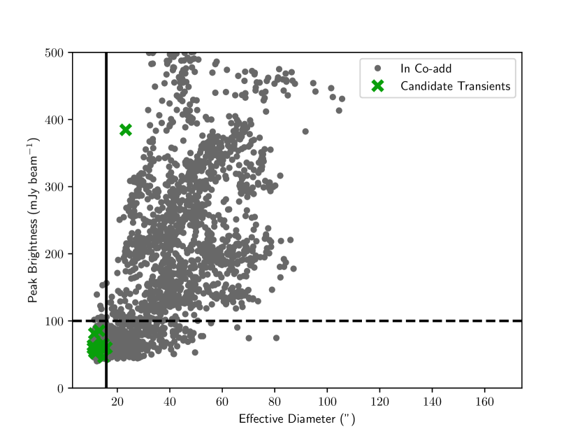
Figure 1: The 850 $\mu$m  peak brightness versus the effective diameter (assuming a circular projection) of all sources identified in all 19 OMC 2/3 epochs. Grey circles indicate sources identified in the co-add that are being analysed by the current pipeline. Green X’s indicate candidate transient sources which do not appear in the co-add (at the level of 5$\sigma_{rms}$) but do appear in at least one epoch. A horizontal (dashed) line has been drawn at $100\mathrm{\>mJy/beam}\sim 10\sigma_{\mathrm{rms}}$. The vertical (solid) line represents the effective 850 $\mu$m beam FWHM after Gaussian smoothing.

Figure 1 shows the 850 $\mu$m  source peak (the maximum pixel value in each source footprint) of all the sources detected in the OMC 2/3 co-add (grey) versus the effective diameter. The effective diameter of a source is calculated by measuring the total area in the identified clump footprint and assuming a projected circular symmetry. Since this method takes into account the full clump size (and not the brightness profile), unresolved sources will appear larger than the beam FWHM while false detections due to residual correlated noise in the final image will appear smaller than the beam FWHM. The circular symmetry assumption holds well for compact (approximately beam-sized) objects. Also included (green) are the sources detected only in individual epochs. Several faint, spurious sources that do not appear at the level of 5$\sigma_{rms}$ in the co-add and are smaller than the beam are detected in single epochs. A full, multi-region analysis of candidate transients like these will be presented by Lalchand et al. (in prep).

One unresolved source, however, is a clear outlier. This source is detected at (R.A., Decl.) = (5:35:17.94,$-5$:16:11) on 2016-11-26 (UT), with an initial 850 $\mu$m  source peak of $384\mathrm{\>mJy\>beam}^{-1}$ in an observation that had a background noise level of $\sigma_{\mathrm{rms}}=9.74\mathrm{\>mJy\>beam}^{-1}$ (SNR = 39). This flux, however, is underestimated as it was measured before the image was re-reduced with an appropriate mask (see Section 2.2). The 2016-11-26 epoch is the only image with a detection of this source. The source was not identified in our initial measurements of variability from the first 11 epochs of the survey (Johnstone et al., 2018) because negative bowling in the region of JW 566 led to an average source brightness of $\sim 0.8\mathrm{\>mJy\>beam}^{-1}$ at the peak pixel location.

The position of this candidate transient peak is within $2.4\arcsec$ of the position of JW 566 (Jones & Walker, 1988), a K7+M1.5 T Tauri binary system with a projected separation of $0\farcs 86$ (Daemgen et al., 2012). It has been classified as a “Disk” by Megeath et al. (2012) based on its mid-infrared colours.

4 A Sub-mm Flare of JW 566

4.1 Detecting the flare at 850 $\mu$m

Out of 20 epochs of SCUBA-2 imaging, only one (2016-11-26) shows bright, unresolved 850 $\mu$m  emission at the location of JW 566 (see Table 1 and Figure 2). Figure 2 presents a light curve derived from extracting the value of the pixel at the peak location of JW 566. The uncertainties are calculated by measuring the average pixel variance in a $20\times 20$ pixel box centered on the source. Figure 3 shows that emission is not detected at this position in the previous image obtained six days earlier, or in the subsequent image obtained three months later. After co-adding all 18 Transient Survey epochs without a detection, the source is still not detected, with a noise of $\sigma_{\mathrm{rms}}=3\mathrm{\>mJy\>beam}^{-1}$ in the co-added map (indicating an upper limit on the flux of $\sim 3\sigma_{\mathrm{rms}}=9\mathrm{\>mJy\>beam}^{-1}$). The source is also not detected in the co-add of the SCUBA-2 images obtained by the JCMT Gould Belt Survey (Ward-Thompson et al., 2007) in 2011, with a sensitivity of $\sim 4\mathrm{\>mJy\>beam}^{-1}$ (Data Release 3; Kirk et al. 2018).

The bright peak associated with JW 566 is detected in the map obtained during a 31-minute observation. The excess emission is consistent with an unresolved object at the (non-smoothed) 14.6$\arcsec$ resolution of the JCMT. The source is best detected in a residual map of the co-add [Figure 3(d)] subtracted from the flare epoch [Figure 3(b)] (after the images were re-reduced with the new mask; see Section 2.2]). The average brightness of the source during our observation is $466\pm 47\mathrm{\>mJy\>beam}^{-1}$ (SNR = 48), as measured by fitting a Gaussian profile to the source in the residual map.

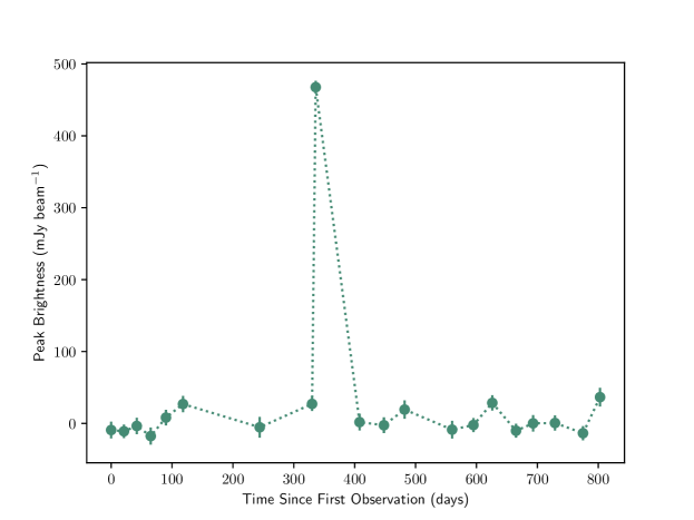
Figure 2: The 850 $\mu$m  light curve of JW 566 over all observed epochs (see Table 1).

Figure 3: 850 $\mu$m  observations of JW 566. Image (a) was observed as part of an engineering program carried out by JCMT staff on the night of 2016-11-20 (UT); the beam is shown in blue. Images (b) and (c) are two consecutive epochs taken as part of the JCMT Transient Survey; the flare occurred on 2016-11-26 [image (b)]. The green triangle represents the position of a known protostar while the magenta squares mark the positions of known Class II YSOs (Megeath et al., 2012). The white circle shows the location of JW 566. Image (d) is a co-add of all 850 $\mu$m  epochs not including 2016-11-26.

4.2 Detecting the flare at 450 $\mu$m

The brightness peak of JW 566 is also detected in the simultaneous 450 $\mu$m images obtained with SCUBA-2. The precipitable water vapor was low on the night of the flare, leading to a noise level of $\sigma_{\mathrm{rms}}=85\mathrm{\>mJy\>beam}^{-1}$. Figure 4 presents the co- added data in image (a), excluding the 2016-11-26 epoch, the 2016-11-26 (flare) epoch in image (b), and a subtraction of image (a) from image (b) in image (c).

Figure 4: 450 $\mu$m  observations of JW 566. The beam size is shown as a blue circle in image (a), the co-added data not including the 2016-11-26 epoch. Image (b) shows the 2016-11-26 epoch when the flare occurred. Image (c) shows the subtraction of image (a) from image (b). Compact structure is obvious in the residual.

As in the case of the 850 $\mu$m  observations, there is no indication of significant emission correlated with the position of JW 566 in any other SCUBA-2 image. A 2-dimensional Gaussian profile fit to the residual 450 $\mu$m  image yields a source peak of $500\pm 107\mathrm{\>mJy\>beam}^{-1}$ (the detection has a SNR=6; see Section 2.2 for more information about the uncertainty).

4.3 Minute to Minute Variability at 850 $\mu$m

Since JW 566 is not detected in the engineering data, 6 days prior to the flare, the source must vary on timescales shorter than one week. In this section, we analyze the light curve of the bright emission peak in nine separate intervals within the 31.12 minute integration of 2016-11-26. In each interval, the source is detected with a SNR between 5 and 25 and is fit with a 2-dimensional Gaussian profile to measure the source peak.

Figure 5: The 850 $\mu$m  peak brightness of JW 566 (top left) along with 5 typical sources in the brightness range displayed by JW 566 throughout the 31 minute integration. The sources were selected from different locations around the OMC 2/3 field. The light curve standard deviations are shown by the shaded regions in each plot. The average standard deviation of the non-varying sources (9.7%) is overlaid on JW 566’s light curve.

Figure 5 shows a dramatic decay in brightness during the 31 minute integration. The emission from JW 566 appears to already be in the dimming phase of the outburst, with an initial peak of $773\mathrm{\>mJy\>beam}^{-1}$ that drops to $400\mathrm{\>mJy\>beam}^{-1}$ by the end of the observation. The uncertainties for each measurement are calculated by measuring the square root average pixel variance in a $20\times 20$ pixel box centered on the source.

To confirm that this brightness decrease is significant, we also analyse the light curves of 5 non-varying unresolved sources with fluxes sampling the range of JW 566 in this epoch. Subdividing the raw time stream was performed in the same way individually for each source as it was for JW 566. Data points with abnormally high variances due to their proximity to the edge of the map or the uncertainty in surrounding, large-scale structure have been discarded. All of these sources are consistent with a constant flux during the 31-minute observation. The average standard deviation of the non-varying sources is 9.7%. The lightcurve of JW 566 is monotonically decreasing and has a standard deviation of 23.2%, more than twice the average value of the non-varying sources. At 450 $\mu$m, the noise is too high to perform a similar analysis.

5 Discussion

Young stars are known to undergo large, short-lived (timescales of hours to days) outbursts detectable at millimetre and centimetre wavelengths (Bower et al., 2003; Furuya et al., 2003; Massi et al., 2006; Salter et al., 2010; Forbrich et al., 2017b). Flare studies tend to focus on these frequencies, leaving the sub-mm frequency space of JCMT largely unexplored.

At a distance of 389 pc, the measured 850 $\mu$m  flux ($466\mathrm{\>mJy\>beam}^{-1}$) corresponds to a radio luminosity of $L_{\nu}=8\times 10^{19}\mathrm{\>erg\>s^{-1}\>Hz^{-1}}$. A natural comparison point for this result is with the 2003 outburst event of the T Tauri star GMR-A in the Orion Nebula (Bower et al. 2003; see also Furuya et al. 2003). GMR-A had a radio luminosity of $L_{\nu}=3\times 10^{19}\mathrm{\>erg\>s^{-1}\>Hz^{-1}}$ at 86 GHz (assuming the same distance of 389 pc), which makes the JW 566 flare an order of magnitude brighter in terms of $\nu L_{\nu}$. Salter et al. (2008) and Massi et al. (2006) observed flares associated with the DQ Tau binary system at 115 GHz and the V773 Tau quadruplet at 90 GHz, respectively, with radio luminosities of $\sim 6\times 10^{19}\mathrm{\>erg\>s^{-1}\>Hz^{-1}}$. If the flare associated with JW 566 follows the X-ray/radio luminosity correlation (see, for example, Güdel, 2002), then it is 10 orders of magnitude brighter than a typical solar flare. It is plausible that this is the most luminous flare ever recorded in a young star. In the future, coordinated observations are required at 450 $\mu$m, 850 $\mu$m, and other wavelengths to reveal the relationship between the fluxes at different energy regimes.

The OMC 2/3 field has been observed with SCUBA-2 for 10 hours since December 26, 2015, and this is the first significant flare event of its kind discovered in those data. In total, there are $\sim 600$ known (Spitzer identified; Megeath et al. 2012) Class II (disk) objects present in the field of view. Therefore, the current detection rate of flare events of this magnitude is $1/(600\mathrm{\>stars}\times 10\mathrm{\>hrs})\approx 1-2\mathrm{\>yr}^{-1}\mathrm{\>star}^{-1}$. It is likely that there is a luminosity function for submillimetre flares that scales as a power law, $N\propto L^{\beta}$, where $\beta<0$. More and deeper observations of this field, including 7 additional hours from our Transient survey by February 2020, will allow us to measure the flare rate over a wide range of luminosities. Additionally, we will be able to perform a more complete search by detecting fainter, longer timescale events by co-adding subsets of the data.

The detection of a coronal flare at sub-mm wavelengths adds another source of uncertainty in the measurement of disk masses (e.g. Pascucci et al., 2016). While sub-mm emission from most sources is produced by the thermal dust continuum emission within the protoplanetary disks, any unexpected emission from sources thought to be diskless should be tested to evaluate whether flaring may explain the emission. Indeed, unresolved 1.3mm continuum emission from Prox Cen was initially interpreted as an indication of a candidate disk (Anglada et al., 2017) but later traced to a stellar flare (MacGregor et al., 2018).

5.1 Previous Observations of JW 566

The JW 566 binary system ($0\farcs 86$ projected separation) has a disk around at least one of the components (Megeath et al., 2012). Daemgen et al. (2012) detected accretion around the K7 primary star but not the M1.5 secondary star. High-resolution optical spectra of JW 566 are not available, so it is unknown whether one or both stars are spectroscopic binaries. Interactions between the magnetospheres of close binaries are thought to excite coronal flares in DQ Tau (Salter et al., 2010) and perhaps other young stars.

Previous X-ray and radio observations demonstrate coronal flares from JW 566, as expected for young low-mass stars. Kounkel et al. (2014) classify the source as variable at both 4.5 and 7.5 GHz. In addition, JW 566 is a known X-ray source (Gagne et al., 1995; Garmire et al., 2000; Feigelson et al., 2002; Getman et al., 2005), with variability on timescales of hours. The JW 566 binary is one of the most luminous X-ray sources, with $L_{X}=10^{31}$ erg s¹, for its mass range in the COUP X-ray monitoring survey of the Orion Nebula (Getman et al., 2005). The extreme brightness is caused by a combination of saturated X-ray emission, with $\log L_{X}/L_{bol}=-3$, and large radii as measured by Daemgen et al. (2012). The X-ray emission is harder than average but not extreme among the COUP sample.

The source is detected in a 3 $\mathrm{\>mm}$ continuum image obtained by ALMA on 2015-12-26 (Hacar et al. 2018; see Figure 6). The 3 mm flux is measured to be $0.6\mathrm{\>mJy}$, yielding a SNR of 5.7. This presumably-quiescent flux is a factor of $8\times 10^{2}$ fainter than the 850 $\mu$m  continuum measurement of the flare, assuming a spectral index of 1. If the 3 mm flux is produced by the disk, a spectral index of $\sim 2.3$ (e.g. Ricci et al., 2010) would lead to an 850 $\mu$m flux of $\sim 10\mathrm{\>mJy\>beam}^{-1}$, very close to our current detection limit in the co-added image and within the flux range expected for disks in nearby star-forming regions (e.g. Ansdell et al., 2016; Pascucci et al., 2016).

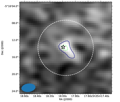
Figure 6: 3 mm continuum ALMA detection of JW 566 (star symbol). Contours are drawn at $3\sigma$ and $5\sigma$. The dashed circle indicates the size of the SCUBA-2 850 $\mu$m  beam FWHM. The beam is displayed in the lower left.

Significant variability has not been detected at wavelengths other than millimetres and the X-rays, including in the optical, $JHK_{S}$ (Tsujimoto et al., 2003; Skrutskie et al., 2006; Ali & Depoy, 1995), at 3.6 and 4.5 $\mu$m (Morales-Calderón et al., 2011), or in the far-IR (Billot et al., 2012). Unfortunately, we do not know of other available data at optical, infrared, or radio wavelengths at the time of this observation.

5.2 The Nature of JW 566’s Flare

Based on the measured source fluxes at 450 $\mu$m  (666 GHz, $f_{666}=500\pm 107\mathrm{\>mJy\>beam}^{-1}$) and 850 $\mu$m  (352 GHz, $f_{352}=466\pm 46.6\mathrm{\>mJy\>beam}^{-1}$) we calculate a spectral index

$$\alpha=\frac{\left(\mathrm{log}(f_{666})\pm\frac{\Delta f_{666}}{f_{666}\mathrm{ln}(10)}\right)-\left(\mathrm{log}(f_{352})\pm\frac{\Delta f_{352}}{f_{352}\mathrm{ln}(10)}\right)}{\mathrm{log}(666\mathrm{\>GHz})-\mathrm{log}(352\mathrm{\>GHz})},$$ (1)

where $\Delta f_{\nu}$ represents the uncertainty in the fluxes, of $\alpha=0.11\pm 0.49$ over these wavelengths. While this value is consistent with non-thermal emission, the spectral index itself is not sufficient to discriminate the emission mechanism.

The brightness temperature, $T_{b}$ can be approximated by

$$T_{b}\sim\left(\frac{1}{2k_{B}}\right)\times\lambda^{2}\Delta S\times\left(\frac{D}{c\Delta t}\right)^{2}$$ (2)

where $k_{B}$ is Boltzmann’s constant, $\Delta S$ is the change in flux over time $\Delta t$, $\lambda$ is the wavelength, $D$ is the distance to the source (389 pc), and $c$ is the speed of light. The change in 850 $\mu$m  flux ($\Delta S$) and its corresponding time frame ($\Delta t$) are derived from the light curve presented in Figure 5 with values of $373\mathrm{\>mJy}$ (mJy = mJy beam^-1, for point sources) and $1661\mathrm{\>sec}$, respectively. This results in a brightness temperature of $T_{b}\sim 6\times 10^{4}\mathrm{\>K}$ and a light crossing distance of 3.3 AU. Constraining the angular scale to a stellar radius of $R_{\star}=2.5\mathrm{\>R}_{\odot}$ (the average radius of the two components in the JW 566 binary system; Daemgen et al., 2012) rather than $c\Delta t$, results in an estimate of the upper range of the brightness temperature of $T_{b}\sim 5\times 10^{9}\mathrm{\>K}$, though the origin of the flare could indeed be generated by a region smaller in scale than $R_{\star}=2.5\mathrm{\>R}_{\odot}$. With a projected separation of 335 AU, it is very unlikely that an inter-binary interaction is occurring among the known components. These calculations strongly favour non-thermal emission. The most likely scenario is that the flare was caused by gyrosynchrotron/synchrotron radiation emitted by a reconnection event in the strong magnetic fields present in the corona of these young stars (see, e.g., Salter et al., 2010). This magnetic reconnection briefly energizes non-thermal particles which appears as a flare. The detection of such an event at 850 $\mu$m  suggests a very high energy acceleration of electrons. Polarimetry data is required to separately constrain the contributions of gyrosynchrotron and synchrotron emission; such data, however, are not available for this event.

6 Summary

In this paper, we presented 450 $\mu$m  and 850 $\mu$m  SCUBA-2 observations of a bright flare associated with the T Tauri binary system JW 566 (R.A., Decl. = 5:35:17.94,$-5$:16:11, J2000) obtained by the JCMT Transient Survey on 2016-11-26 (UT). The flare is measured to have a flux of $466\pm 47\mathrm{\>mJy\>beam}^{-1}$ at 850 $\mu$m  and $500\pm 107\mathrm{\>mJy\>beam}^{-1}$ at 450 $\mu$m , averaged over the observation (see Sections 4.1 and 4.2). We subdivided the 31 minute integration into nine intervals based on when the telescope scanned over the source and found a monotonic decrease of $337\mathrm{\>mJy\>beam}^{-1}$ over $1661\mathrm{\>sec}$ (see Section 4.3). Constraining the size scale of the flare origin to the light crossing time of our observation and to the stellar radius of one of the binary components results in a range of brightness temperatures between $T_{b}\sim 6\times 10^{4}\mathrm{\>K}$ and $T_{b}\sim 5\times 10^{9}\mathrm{\>K}$ (see Section 5.2). The flat spectral index, the short variability timescale, and a large $T_{b}$ strongly indicate the flare is a result of gyrosynchrotron/synchrotron emission, likely caused by a magnetic reconnection event.

The true timescale of the flare remains unknown, as there are no data available at other wavelengths during the time of our observation. The JCMT Transient Survey will continue through January 2020, increasing the number of observations of the OMC 2/3 field by a factor of $\sim 1.7$. Therefore, it is plausible another burst of a similar magnitude will be detected. With new variable source detection methods Lalchand et al. (in prep.), we will be able to identify future events within $\sim 24\mathrm{\>hours}$ of the data being taken by the telescope in order to perform follow-up observations.

References

- Ali & Depoy (1995) Ali, B., & Depoy, D. L. 1995, AJ, 109, 709
- Anglada et al. (2017) Anglada, G., Amado, P. J., Ortiz, J. L., et al. 2017, ApJ, 850, L6
- Ansdell et al. (2016) Ansdell, M., Williams, J. P., van der Marel, N., et al. 2016, ApJ, 828, 46
- Astropy Collaboration et al. (2013) Astropy Collaboration, Robitaille, T. P., Tollerud, E. J., et al. 2013, A&A, 558, A33
- Benz & Güdel (2010) Benz, A. O., & Güdel, M. 2010, ARA&A, 48, 241
- Berry (2015) Berry, D. S. 2015, Astronomy and Computing, 10, 22
- Billot et al. (2012) Billot, N., Morales-Calderón, M., Stauffer, J. R., Megeath, S. T., & Whitney, B. 2012, ApJ, 753, L35
- Bower et al. (2003) Bower, G. C., Plambeck, R. L., Bolatto, A., et al. 2003, ApJ, 598, 1140
- Buckle et al. (2009) Buckle, J. V., Hills, R. E., Smith, H., et al. 2009, MNRAS, 399, 1026
- Chapin et al. (2013) Chapin, E. L., Berry, D. S., Gibb, A. G., et al. 2013, MNRAS, 430, 2545
- Cleeves et al. (2017) Cleeves, L. I., Bergin, E. A., Öberg, K. I., et al. 2017, ApJ, 843, L3
- Coudé et al. (2016) Coudé, S., Bastien, P., Kirk, H., et al. 2016, MNRAS, 457, 2139
- Currie et al. (2014) Currie, M. J., Berry, D. S., Jenness, T., et al. 2014, in Astronomical Society of the Pacific Conference Series, Vol. 485, Astronomical Data Analysis Software and Systems XXIII, ed. N. Manset & P. Forshay, 391
- Daemgen et al. (2012) Daemgen, S., Correia, S., & Petr-Gotzens, M. G. 2012, A&A, 540, A46
- Dempsey et al. (2013) Dempsey, J. T., Friberg, P., Jenness, T., et al. 2013, MNRAS, 430, 2534
- Drabek et al. (2012) Drabek, E., Hatchell, J., Friberg, P., et al. 2012, MNRAS, 426, 23
- Feigelson et al. (2002) Feigelson, E. D., Garmire, G. P., & Pravdo, S. H. 2002, ApJ, 572, 335
- Feigelson & Montmerle (1999) Feigelson, E. D., & Montmerle, T. 1999, ARA&A, 37, 363
- Forbrich et al. (2008) Forbrich, J., Menten, K. M., & Reid, M. J. 2008, A&A, 477, 267
- Forbrich et al. (2017a) Forbrich, J., Reid, M. J., Menten, K. M., et al. 2017a, ApJ, 844, 109
- Forbrich et al. (2017b) —. 2017b, ApJ, 844, 109
- Forbrich et al. (2016) Forbrich, J., Rivilla, V. M., Menten, K. M., et al. 2016, ApJ, 822, 93
- Fraschetti et al. (2018) Fraschetti, F., Drake, J. J., Cohen, O., & Garraffo, C. 2018, ApJ, 853, 112
- Furuya et al. (2003) Furuya, R. S., Shinnaga, H., Nakanishi, K., Momose, M., & Saito, M. 2003, PASJ, 55, L83
- Gagne et al. (1995) Gagne, M., Caillault, J.-P., & Stauffer, J. R. 1995, ApJ, 445, 280
- Gaia Collaboration et al. (2018) Gaia Collaboration, Brown, A. G. A., Vallenari, A., et al. 2018, ArXiv e-prints, arXiv:1804.09365
- Garmire et al. (2000) Garmire, G., Feigelson, E. D., Broos, P., et al. 2000, AJ, 120, 1426
- Getman et al. (2008a) Getman, K. V., Feigelson, E. D., Broos, P. S., Micela, G., & Garmire, G. P. 2008a, ApJ, 688, 418
- Getman et al. (2005) Getman, K. V., Feigelson, E. D., Grosso, N., et al. 2005, ApJS, 160, 353
- Getman et al. (2008b) Getman, K. V., Feigelson, E. D., Micela, G., et al. 2008b, ApJ, 688, 437
- Gibb et al. (2013) Gibb, A. G., Jenness, T., & Economou, F. 2013, PICARD - A PIpeline for Combining and Analyzing Reduced Data, Starlink User Note 265, Joint Astronomy Centre, Hilo, HI., ,
- Glassgold et al. (2004) Glassgold, A. E., Najita, J., & Igea, J. 2004, ApJ, 615, 972
- Güdel (2002) Güdel, M. 2002, ARA&A, 40, 217
- Güdel & Benz (1993) Güdel, M., & Benz, A. O. 1993, ApJ, 405, L63
- Güdel et al. (2014) Güdel, M., Dvorak, R., Erkaev, N., et al. 2014, Protostars and Planets VI, 883
- Hacar et al. (2018) Hacar, A., Tafalla, M., Forbrich, J., et al. 2018, A&A, 610, A77
- Herczeg et al. (2017) Herczeg, G. J., Johnstone, D., Mairs, S., et al. 2017, ApJ, 849, 43
- Holland et al. (2013) Holland, W. S., Bintley, D., Chapin, E. L., et al. 2013, MNRAS, 430, 2513
- Hunter (2007) Hunter, J. D. 2007, Computing In Science & Engineering, 9, 90
- Jenness et al. (2013) Jenness, T., Chapin, E. L., Berry, D. S., et al. 2013, SMURF: SubMillimeter User Reduction Facility, Astrophysics Source Code Library., , , ascl:1310.007:
- Johnstone et al. (2013) Johnstone, D., Hendricks, B., Herczeg, G. J., & Bruderer, S. 2013, ApJ, 765, 133
- Johnstone et al. (2018) Johnstone, D., Herczeg, G. J., Mairs, S., et al. 2018, ApJ, 854, 31
- Jones & Walker (1988) Jones, B. F., & Walker, M. F. 1988, AJ, 95, 1755
- Kackley et al. (2010) Kackley, R., Scott, D., Chapin, E., & Friberg, P. 2010, in Proc. SPIE, ed. T. G. Phillips & J. Zmuidzinas, Vol. 7740, 1. SPIE, Bellingham, WA
- Kirk et al. (2018) Kirk, H., Hatchell, J., Johnstone, D., et al. 2018, ArXiv e-prints, arXiv:1808.07952
- Kounkel et al. (2014) Kounkel, M., Hartmann, L., Loinard, L., et al. 2014, ApJ, 790, 49
- Kounkel et al. (2017) —. 2017, ApJ, 834, 142
- Kounkel et al. (2018) Kounkel, M., Covey, K., Suárez, G., et al. 2018, AJ, 156, 84
- Lammer et al. (2018) Lammer, H., Zerkle, A. L., Gebauer, S., et al. 2018, A&A Rev., 26, 2
- MacGregor et al. (2018) MacGregor, M. A., Weinberger, A. J., Wilner, D. J., Kowalski, A. F., & Cranmer, S. R. 2018, ApJ, 855, L2
- Mairs et al. (2015) Mairs, S., Johnstone, D., Kirk, H., et al. 2015, MNRAS, 454, 2557
- Mairs et al. (2017a) —. 2017a, ApJ, 849, 107
- Mairs et al. (2017b) Mairs, S., Lane, J., Johnstone, D., et al. 2017b, ApJ, 843, 55
- Massi et al. (2006) Massi, M., Forbrich, J., Menten, K. M., et al. 2006, A&A, 453, 959
- Megeath et al. (2012) Megeath, S. T., Gutermuth, R., Muzerolle, J., et al. 2012, AJ, 144, 192
- Morales-Calderón et al. (2011) Morales-Calderón, M., Stauffer, J. R., Hillenbrand, L. A., et al. 2011, ApJ, 733, 50
- Parsons et al. (2018) Parsons, H., Dempsey, J. T., Thomas, H. S., et al. 2018, ApJS, 234, 22
- Pascucci et al. (2016) Pascucci, I., Testi, L., Herczeg, G. J., et al. 2016, ApJ, 831, 125
- Rab et al. (2017) Rab, C., Güdel, M., Padovani, M., et al. 2017, A&A, 603, A96
- Ricci et al. (2010) Ricci, L., Testi, L., Natta, A., et al. 2010, A&A, 512, A15
- Robitaille & Bressert (2012) Robitaille, T., & Bressert, E. 2012, APLpy: Astronomical Plotting Library in Python, Astrophysics Source Code Library, , , ascl:1208.017
- Salter et al. (2008) Salter, D. M., Hogerheijde, M. R., & Blake, G. A. 2008, A&A, 492, L21
- Salter et al. (2010) Salter, D. M., Kóspál, Á., Getman, K. V., et al. 2010, A&A, 521, A32
- Shu et al. (1997) Shu, F. H., Shang, H., Glassgold, A. E., & Lee, T. 1997, Science, 277, 1475
- Skrutskie et al. (2006) Skrutskie, M. F., Cutri, R. M., Stiening, R., et al. 2006, AJ, 131, 1163
- Sossi et al. (2017) Sossi, P. A., Moynier, F., Chaussidon, M., et al. 2017, Nature Astronomy, 1, 0055
- Tsujimoto et al. (2003) Tsujimoto, M., Koyama, K., Kobayashi, N., et al. 2003, AJ, 125, 1537
- Ward-Thompson et al. (2007) Ward-Thompson, D., Di Francesco, J., Hatchell, J., et al. 2007, PASP, 119, 855
- Wenger et al. (2000) Wenger, M., Ochsenbein, F., Egret, D., et al. 2000, A&AS, 143, 9
- Yoo et al. (2017) Yoo, H., Lee, J.-E., Mairs, S., et al. 2017, ApJ, 849, 69