Resistive evolution of toroidal field distributions
and their relation to magnetic clouds

Abstract

We study the resistive evolution of a localized self-organizing magnetohydrodynamic equilibrium. In this configuration the magnetic forces are balanced by a pressure force caused by a toroidal depression in the pressure. Equilibrium is attained when this low pressure region prevents further expansion into the higher-pressure external plasma. We find that, for the parameters investigated, the resistive evolution of the structures follows a universal pattern when rescaled to resistive time. The finite resistivity causes both a decrease in the magnetic field strength and a finite slip of the plasma fluid against the static equilibrium. This slip is caused by a Pfirsch-Schlüter type diffusion, similar to what is seen in tokamak equilibria. The net effect is that the configuration remains in Magnetostatic equilibrium whilst it slowly grows in size. The rotational transform of the structure becomes nearly constant throughout the entire structure, and decreases according to a power law. In simulations this equilibrium is observed when highly tangled field lines relax in a high-pressure (relative to the magnetic field strength) environment, a situation that occurs when the twisted field of a coronal loop is ejected into the interplanetary solar wind. In this paper we relate this localized MHD equilibrium to magnetic clouds in the solar wind.

1 Introduction

Spontaneous self-organization of magnetized plasma lies at the basis of many fascinating phenomena in both fusion reactor operation and astrophysical plasma observations. In such situations, magnetic helicity in the plasma is of crucial importance in determining the evolution of the system. Magnetic helicity is an integral quantity calculated by $H_{\rm m}=\int\bm{A}\cdot\bm{B}\mathrm{d}^{3}x$ where $\bm{A}$ is the vector potential and $\bm{B}=\nabla\times\bm{A}$ is the magnetic field. Helicity was given its name by Moffatt (1969) who recognized its topological interpretation; a measure of the self- and interlinking of magnetic field lines. This notion was extended to non-closing and ergodic field lines by Arnol’d (1986). In a perfectly conducting plasma, the magnetic field can be seen as being ‘frozen in’ and is advected with the fluid motion(Alfvén, 1943; Batchelor, 1950). Since the fluid motions can then only distort and reshape the magnetic field lines, but cannot break or cause unlinking, the conservation of helicity is easily understood from a topological perspective.

In perfectly conducting plasma helicity is exactly conserved (Berger & Field, 1984), whilst in resistive plasma the rate of energy decay is strongly constrained by its presence (Del Sordo et al., 2010). The most famous example where helicity determines a self-organizing process is the Taylor conjecture (Taylor, 1974, 1986) which states that the magnetic field in a toroidally bounded plasma relaxes to a linear-force free state (shown by Woltjer (1958) to be the lowest-energy state) with exactly the same helicity as it started with.

But what state is achieved when a helical plasma relaxes in an environment without a boundary? If the plasma’s fluid pressure is high compared to the magnetic pressure (high plasma $\beta=\frac{p}{B^{2}/2}$), the linking in the initial field gives rise to a self-organized MHD equilibrium where field lines lie on nested toroidal magnetic surfaces (Smiet et al., 2015). The approximately axisymmetric field is in a Grad-Shafranov equilibrium (Shafranov, 1966), and the Lorentz force is balanced by a gradient in pressure. The pressure is lowest on the magnetic axis, which is the field line lying at the center of the nested toroidal magnetic surfaces. In this structure the rotational transform is nearly constant from surface to surface. As a consequence the magnetic field line structure is topologically similar to the mathematical structure of the Hopf fibration (Hopf, 1931) or its generalization to torus knots (Arrayás & Trueba, 2014; Smiet et al., 2015). It should be noted that the Hopf structure has previously also been used in a beautiful paper by Finkelstein and Weil (Finkelstein & Weil, 1978) to generate linked and knotted magnetic fields for astrophysics. The relaxation of the Hopf field to the Grad-Shafranov equilibrium has been shown using topology conserving relaxation in our recent paper (Smiet et al., 2016). It is remarkable that this structure is obtained for a wide class of initially helical fields; it emerges from trefoils (Smiet et al., 2015), twisted rings, and even Borromean linked flux tubes (Candelaresi & Brandenburg, 2011).

The robust generation of this ordered magnetic structure makes it natural to assume that a similar process emerges after the twisted magnetic field of a coronal loop is ejected into the high-beta interplanetary plasma of the solar wind. The pressure in the solar wind at 1 A.U. is of the order of $p=1.4\times 10^{-11}Nm^{-2}$ and the field strength $B=6\times 10^{-9}T$ such that the plasma $\beta=2\mu_{0}p/B^{2}\simeq 1$ (Goedbloed & Poedts, 2004). Such events are called Coronal Mass Ejections (CME’s), and CME’s are correlated with the observation of magnetic clouds (Burlaga, 1991). A magnetic cloud is a localized magnetic structure in the interplanetary plasma with increased magnetic field strength, and where the direction of the field varies by a large angle (Burlaga, 1991). These magnetic signatures are observed by interplanetary sattelites with increasingly accurate magnetic instruments (Raghav & Kule, 2018). Unfortunately due to the low density of probes in the interplanetary medium, high-resolution measurement of the complete magnetic structure in these clouds is challenging.

There are several models for the magnetic structure of these clouds published in literature (Burlaga, 1991). Some models assume the field in the cloud is still magnetically connected to the surface of the sun, but there are several models that assume a localized magnetic field which is created by internal currents and balanced by the external plasma pressure (Vandas et al., 1992; Kumar & Rust, 1996; Burlaga, 1991; Ivanov & Harshiladze, 1985; Garren & Chen, 1994). In this paper we posit the self-organized state identified in (Smiet et al., 2015) as a new model. This model gives different predictions for the structure from the models above.

In this paper, we study the evolution of the self-organizing equilibrium starting from a twisted flux tube. We vary both the resistivity of the simulation as well as the amount of twist in the initial flux tube. The evolution of the structure is governed by two processes. First, the lowering of the magnetic field strength changes the equilibrium condition, such that the depression in pressure becomes smaller. Second, finite resistance breaks the frozen-in condition, allowing the plasma fluid to slip perpendicular to the magnetic field lines of the configuration. The net effect of this is a fluid flow directed towards the region of lowest pressure. The combined effect of these two processes is a structure that grows on a resistive timescale. The magnetic topology, characterized by the rotational transform of the magnetic surfaces, quickly reaches a nearly flat profile with a slight positive curvature. The rotational transform decays according to a power law, the characteristic exponent of which depends on the aspect ratio of the structure.

2 Initial field

Figure 1: Coordinate system used for the construction of the initial magnetic field. The surfaces through which the toroidal flux $\psi_{t}$ and poloidal flux $\psi_{p}$ are defined are shown by the blue and green circles respectively. $\phi$ is the coordinate pointing in the poloidal direction of the torus, and $\theta$ is the coordinate pointing in the toroidal direction. The magnetic axis is given by the red circle located at $R^{*}=1$.

In our previous paper (Smiet et al., 2015), we showed how a self-organizing equilibrium is generated through the chaotic reconnection of linked magnetic flux rings. The violent reconnection and high spatial gradients generated when the flux tubes meet, necessitated a high value of resistivity and low magnetic field strength to numerically resolve.

In this paper we use an initial condition which re-organizes in a much more ordered fashion. The initial field consists of a twisted flux tube with field lines lying on nested toroidal flux surfaces with varying rotational transform. We use cylindrical coordinates $R,z,\theta$ and flux functions $\psi_{p}(R,z)$ and $I(\psi_{p})$. The coordinate system is described in figure 1. Physically $\psi_{p}(R,z)$ represents the poloidal magnetic flux, passing through a circular surface of radius $R$ around the $z$-axis (green circle). $I$ physically represents the total poloidal current, the current through the green, shaded circle. The magnetic field is calculated from the flux functions by the standard methods for axisymmetric fields (Goedbloed et al., 2010):

$$B_{R}=-\frac{1}{R}\frac{\partial\psi_{p}}{\partial z},\quad B_{z}=\frac{1}{R}\frac{\partial\psi_{p}}{\partial R},\quad B_{\theta}=\frac{1}{R}I.$$ (1)

Using this construction guarantees that the magnetic field is divergence free, and that field lines lie on magnetic surfaces of constant $\psi_{p}$.

We choose the following flux function,

$$\psi_{p}=\begin{cases}B_{0}\cos^{4}\left(\frac{\pi}{2}\frac{a}{a_{0}}\right),&a\leq a_{0}\\ 0,&a>a_{0}\end{cases}$$ (2)

where $0<a_{0}<1$ and with $B_{0}$ a scaling parameter that sets the magnetic field strength and

$$a=\sqrt{(1-R)^{2}+z^{2}},$$ (3)

denoting the distance from the unit circle (the circle $R=1,z=0$, indicated in red in figure 1), which is the magnetic axis of this initial condition.

With this choice we can see that $\psi_{p}$ is constant and zero for $a\geq a_{0}$ such that, according to equation (1), the poloidal field vanishes. The magnetic surfaces in the region where $a<a_{0}$ form concentric tori with circular cross section that enclose the magnetic axis.

We can choose any function of $\psi_{p}$ for the toroidal current function $I$, which here we define as:

$$I=\frac{\psi_{p}\pi^{2}}{\imath_{0}^{*}a_{0}^{2}},$$ (4)

where a scaling parameter $\imath_{0}^{*}$ is introduced, named such because it sets the rotational transform on axis, as we will show in Section 2.1. With this choice for $I$ the toroidal magnetic field also vanishes for $a\geq a_{0}$, and thus the field describes an axisymmetric flux tube with major radius $1$ and minor radius $a_{0}$ with $\bm{B}=0$ outside of the tube. Note: We use the convention that a subscript zero denotes a value at time $t=0$, and a superscript asterisk denotes that the quantity is measured on the magnetic axis.

2.1 Rotational transform profile

The winding of field lines in a toroidal magnetic structure is quantified by the rotational transform $\imath$ or its inverse, the safety factor $q$. The rotational transform geometrically represents the ratio of the number of times a field line wraps around the poloidal direction of a torus to the number of times it winds around the toroidal direction. The safety factor can be calculated using the well-known formula (Wesson & Campbell, 2011):

$$q=\frac{1}{2\pi}\oint\frac{1}{R}\frac{B_{\theta}}{B_{p}}{\rm d}{}l,$$ (5)

where $B_{p}$ is the magnitude of the poloidal magnetic field $B_{R}\hat{R}+B_{z}\hat{z}$, and the integration is carried out over a constant $\theta$ cross section of a magnetic surface $(\psi_{p}=\text{ const.})$. This integration path is indicated by the blue circle in figure 1.

The poloidal magnetic flux enclosed between concentric magnetic surfaces of radii $a$ and $a$ + $\mathrm{d}a$ is $\mathrm{d}a2\pi RB_{p}.$ Hence conservation of poloidal flux implies that $RB_{p}$ is constant on each surface. Evaluating the poloidal field at $z=0,R\geq 1$, where $\frac{\partial\psi_{p}}{\partial z}=0$ and $\frac{\partial\psi_{p}}{\partial R}=\frac{\partial\psi_{p}}{\partial a}$ its value in the direction of the poloidal vector $\phi$ is equal to

$$RB_{p}=\frac{\partial\psi_{p}}{\partial a}=B_{0}\frac{2\pi}{a_{0}}\cos^{3}\left(\frac{a\pi}{2a_{0}}\right)\sin\left(\frac{a\pi}{2a_{0}}\right).$$ (6)

The toroidal magnetic field is:

$$B_{\theta}=B_{0}\frac{\pi^{2}\cos^{4}\left(\frac{\pi a}{2a_{0}}\right)}{R\imath_{0}^{*}a_{0}^{2}}.$$ (7)

On the magnetic surfaces the parameter $a$ is a constant, so filling this in equation (5) becomes:

$$q(a)=\frac{\cos\left(\frac{a\pi}{2a_{0}}\right)}{4\imath_{0}^{*}a_{0}\sin\left(\frac{a\pi}{2a_{0}}\right)}\ \ \oint\frac{1}{R}{\rm d}{}l.$$ (8)

Using $\phi$ to parametrize the integral over the surface at $a$, and the identities $R=1+a\cos(\phi)$ and ${\rm d}{}l=a{\rm d}{}\phi$, we get:

$$\oint\frac{1}{R}{\rm d}{}l=\int_{0}^{2\pi}\frac{a}{1+a\cos(\phi)}{\rm d}{}\phi=\frac{2\pi a}{\sqrt{1-a^{2}}}.$$ (9)

This gives us the safety factor

$$q(a)=\frac{\frac{a\pi}{2a_{0}}\cot\left(\frac{a\pi}{2a_{0}}\right)}{\imath_{0}^{*}\sqrt{1-a^{2}}},$$ (10)

and hence a rotational transform of:

$$\imath(a)=\imath_{0}^{*}\sqrt{1-a^{2}}\frac{\tan\left(\frac{a\pi}{2a_{0}}\right)}{\frac{a\pi}{2a_{0}}}.$$ (11)

The rotational transform profile is flat near the magnetic axis, and increases to infinity when $a\rightarrow a_{0}$. At the magnetic axis the rotational transform is given by

$$\lim_{a\rightarrow 0}\imath(a)=\imath_{0}^{*}.$$ (12)

The initial condition is thus an axisymmetric, twisted magnetic flux tube lying in the $R,\!\theta$-plane. We can change the twist of the magnetic field lines in the initial condition by tuning the parameter $\imath_{0}^{*}$, and the toroidal magnetic field strength with the parameter $B_{0}$.

3 Time evolution

Figure 2: Resistive evolution of the magnetic structure. Parameters are: $\imath_{0}^{*}=3$, $B_{0}=0.05$ and $\eta=2\times 10^{-4}$. Top row: Cross sections in the $R,\!z$-plane at different times. The color indicates the rotational transform of a field line starting at that position. The configuration is seen to first contract onto the $z$-axis and then slowly expand. The horizontal lines indicates the location where the rotational transform, shown in the bottom panel, is taken. The cross sections shown are at times which correspond with the top six colored lines in the bottom panel and are exponentially spaced. Bottom panel: Evolution of the rotational transform profile and the location of the magnetic axis. The black line along the center is the location of the magnetic axis. The colored part around the black line indicates the time at which the magnetic axis was at that location. The top six colored lines correspond to the six cross sections shown in the top row, and their color again indicates the time at which that rotational transform profile was calculated. The red dashed line is the analytical result of equation (11). We can see that the configuration quickly reaches a nearly flat rotational transform profile and subsequently evolves self-similarly.

We simulate the time evolution of the helical magnetic fields numerically using the resistive, viscous, compressible isothermal MHD equations. The equations are solved using the PENCIL-CODE (http://pencil-code.nordita.org/). This is a highly used solver of the MHD equations on a fixed Eulerian grid often used for astrophysical applications (Brandenburg & Dobler, 2002; Haugen et al., 2004; Johansen et al., 2007).

The PENCIL-CODE solves the MHD equations in terms of the vector potential $\bm{A}$, ensuring that the magnetic field remains divergence free. The equation of motion solved is:

$$\frac{D\mbox{\boldmath$v$}{}}{Dt}=-c_{\rm s}^{2}\nabla\ln\rho+\mbox{\boldmath$j$}{}\times\bm{B}/\rho+\mathbf{F}_{\rm visc}/\rho$$ (13)

where $\bm{B}$ is calculated through $\bm{B}=\nabla\times\bm{A}$ and the current $\mbox{\boldmath$j$}{}=\nabla\times\bm{B}$. The fluid velocity is $v$ and the convective derivative is denoted by $\tfrac{D}{Dt}\equiv\tfrac{\partial}{\partial t}+\mbox{\boldmath$v$}{}\cdot\nabla$. The simulation is isothermal, so the pressure is related to the density by $p=\rho c_{s}^{2}$ where $c_{s}^{2}$ is the sound speed (set to unity). The viscous force $\mathbf{F}_{\rm visc}$ is calculated using the rate of strain tensor $\mathsfbi{S}$ whose indices are given by $S_{ij}=\tfrac{1}{2}(\frac{\partial u_{i}}{\partial x_{j}}+\frac{\partial u_{j}}{\partial x_{i}})-\tfrac{1}{3}\delta_{ij}\nabla\cdot\mbox{\boldmath$v$}{}.$ through the equation:

$$\mathbf{F}_{\rm visc}=\nabla\cdot 2\nu\rho\mathsfbi{S},$$ (14)

The continuity equation is implemented in terms of the logarithm of the density $\rho$ as follows

$$\frac{D\ln\rho}{Dt}=-\nabla\cdot\mbox{\boldmath$v$}{}.$$ (15)

Since the plasma is modeled as isothermal the equation of state does not need to be solved, so the final equation is the induction equation, which in terms of the vector potential becomes

$$\frac{\partial\mathbf{A}}{\partial t}=\mbox{\boldmath$v$}{}\times\mathbf{B}+\eta\nabla^{2}\mathbf{A}$$ (16)

where we have chosen the Weyl gauge for $\bm{A}$ to simplify the equation and $\eta$ is the resistivity.

These equations are solved on an Eulerian grid of $256^{3}$ grid points in a simulation box of size 5. This puts the boundary at $R=2.5$. The simulation is run using perpendicular-field boundary conditions, by imposing a vanishing parallel component of the magnetic field on the boundary. This boundary condition allows magnetic field to escape from the simulation volume. The full field information is saved every 5 simulation time steps. The simulation is initialized with a constant pressure $p=1$ throughout the volume and the velocity field is zero. The Alfvén speed $v_{A}$ in the initial field is ranges from 0.28 to 1.1 (on axis) $B_{0}$ is varied between 0.05 and 0.2 and this makes it the same order of magnitude as the sound speed $c_{s}^{2}=1$. We scale the time to a resistive timescale using $t_{\eta}=R^{2}_{\rm char}/\eta$. For the characteristic length scale $R_{\rm char}$ we choose the distance of the magnetic axis from the origin in the initial field, $R^{*}(0)=1$. The viscosity parameter $\nu$ is set to $2\times 10^{-4}$ whereas the resistivity $\eta$ is varied from $2\times 10^{-4}$ to almost an order of magnitude lower. This makes the magnetic Prandtl number equal to unity or larger

In our analysis of the simulation results we wish to extract the topological properties of the magnetic field structures. We do this by means of a Runge-Kutta field line integration. From the resultant field line traces we can find the magnetic axis and the rotational transform of the field line if it lies on a toroidal surface. One implementation of this field line tracing is described in the supplemental material of (Smiet et al., 2015). This method was used in Section 4-5.

Furthermore we have developed an alternative implementation in CUDA to run on graphics hardware. The hardware accelerated trilinear interpolation and massive parallelization allow for a high speedup compared to CPU-based field line tracing. In the $(R,\!0,\!z)$-plane field lines are traced from a $1024\times 1024$ grid and for every field line the rotational transform is calculated.

The evolution of the rotational transform profile can be seen in supplemental video 1. This video shows the color-coded rotational transform, similar to the top row in figure 2, for all times sequentially. Additionally, this video gives a good indication of how the magnetic structure evolves in time.

The results of this analysis are shown in figure 2, top row, for the field with $\imath_{0}^{*}$=3, $B_{0}=0.05$ and $\eta=2\times 10^{-4}$. Every single pixel in these images is the result of calculating the rotational transform of a field line trace. In this run the magnetic field remains axisymmetric and the magnetic axis remains in the plane defined by $z=0$. This is the case for all runs presented in this paper, even though these symmetries are in no way enforced by the computational procedure. With higher values of $\imath_{0}^{*}$ the structure can become susceptible to a nonaxisymmetric kink instability, which will be the subject of a future publication.

Figure 2 (bottom) shows the rotational transform profile at different times during the evolution of the configuration. The rotational transform profile quickly shifts from positively curved to nearly flat with a slight negative curvature. After this initial phase the rotational transform profile remains nearly constant in space but decreases in time. In the next sections we will study this decay.

In the rest of the paper we will analyze the change in rotational transform and the location of the magnetic axis in time. We will look at the effect of changing the resistivity $\eta$ and the initial rotational transform $\imath_{0}^{*}$.

4 Resistive growth and decay of rotational transform

In figure 2 it is seen that the magnetic axis first shifts inwards and then slowly moves back out. We follow this dynamic of the magnetic structure by extracting $R^{*}$, the distance from the origin to the magnetic axis as a function of resistive time. This is done for three different values of $\imath_{0}^{*}$ at constant $\eta=4\times 10^{-4}$. The results are shown in figure 3. The structure relaxes to a radius which depends on $\imath_{0}^{*}$, and then slowly increases in size.

As the structure grows, it has reached its equilibrium: the magnetic pressure pushes outwards, but the expansion is halted by the strong external pressure. A lowering of the pressure is observed in a toroidal region as we show here in figure 6, and is described in more detail in (Smiet et al., 2015, 2016).

Figure 3: Position of the magnetic axis in time for different values of $\imath_{0}^{*}$. The magnetic axis performs a damped oscillatory motion towards an equilibrium position which depends on the initial rotational transform, and then slowly grows. The parameters $B_{0}=0.05$ and $\eta=2\times 10^{-4}$ are fixed with $\imath_{0}^{*}$ varied as shown.

We can understand this initial relaxation qualitatively from the interplay between magnetic tension and magnetic pressure. Since the initial pressure is constant and the velocity is zero the initial motion of the fluid is purely due to the Lorentz force $\mbox{\boldmath$j$}{}\times\bm{B}$. A high value of $\imath_{0}^{*}$ results in a high poloidal field, and magnetic tension along the field lines squeezes the configuration into an expanding ring. The case of a low rotational transform will result in stronger toroidal field, and the magnetic tension will cause the structure to contract. In figure 3 we see that higher $\imath_{0}^{*}$ leads to an initial expansion, and an equilibrium with a value of $R^{*}$ larger than $1$, whereas low values of $\imath_{0}^{*}$ lead to an initial contraction. $R^{*}$ performs a damped Alfvénic oscillation to the equilibrium position, and then slowly grows.

The later evolution of the structure proceeds on a purely resistive time scale. This is tested by simulating the evolution of the field with the parameters $\imath_{0}^{*}=3$, $B_{0}=0.05$ and varying resistivity $\eta=2\times 10^{-4},1\times 10^{-4}$, and $5\times 10^{-5}$. When rescaled to resistive time the growth of the structure and the change in rotational transform all collapse to a single curve indicating a universal growth mechanism, as shown in figure 4.

Figure 4: $\imath^{*}(t)$ and $R^{*}(t)$ as a function of resistive time for several different values of resistivity $\eta$. The initial rotational transform is set to $\imath_{0}^{*}=3$, and magnetic field strength $B_{0}=0.05$. The change of the rotational transform and the radius of the structure all behave identically on a resistive time scale.

The magnetic field strength $B_{0}$ does not affect the equilibrium reached or the rate of growth and change in rotational transform exhibited by these configurations. This is shown in figure 5, where the field with $B_{0}=0.05$ and $B_{0}=0.2$ are compared for $\imath_{0}^{*}=3$, $\eta=2\times 10^{-4}$. Despite a factor $4$ difference in the magnetic field strength the structures behave identically except for the initial reconfiguration towards the equilibrium. As this reconfiguration is mediated by magnetic forces, it proceeds on an Alfvénic timescale linear in the magnetic field, $\tau_{A}=\frac{B}{\sqrt{\rho}}$. It is therefore not surprising that the oscillation to the equilibrium $R^{*}$ lasts about 4 times longer for the field where the magnetic amplitude is a quarter of the strength.

Figure 5: Magnetic decay of topologically identical structures with different initial magnetic field strength $B_{0}$. Despite the difference in magnetic field strength the change in rotational transform proceeds at exactly the same rate with identical equilibrium. Note that the initial oscillations towards the equilibrium radius occur on the Alfvénic timescale: the oscillations to the equilibrium configuration proceed at a four times faster rate when $B_{0}=0.2$ then when $B_{0}=0.05$. In these runs $\imath_{0}^{*}=3$ and $\eta=2\times 10^{-4}$

5 Pfirsch-Schlüter diffusion

We can understand the structure growth and change in rotational transform through the effect of finite resistivity on the plasma and the lowering of magnetic field strength through resistivity. In a perfectly conducting plasma a magnetic field is effectively ‘frozen-in’ and moves with the fluid motion (Alfvén, 1943; Batchelor, 1950; Priest & Forbes, 2000), thus there can be no net flow of fluid perpendicular to the field lines if the magnetic configuration is static. When resistivity is included this restriction is lifted and the fluid can slip against the static magnetic field lines. Field line slip is observed in many different scenarios and is one of the driving mechanisms behind $2D$ reconnection (Kulsrud, 2011). In the toroidal geometry of an operating tokamak, field line slip gives rise to slow diffusion out of the toroidal flux surfaces. This process is called Pfirsch-Schlüter diffusion (Wesson & Campbell, 2011). This Pfirsch-Schlüter flow is directed outwards, in the direction of the pressure gradient.

In the self-organized structures considered here a similar magnetic slip causes a diffusion of plasma fluid into the magnetic structure. This is shown in figure 6, where the flow field is plotted along the $x$-axis together with the pressure profile. The magnetic axis is located at the minimum of the pressure, and it is clearly seen how there is net fluid flow directed towards the magnetic axis. We suggest that the slight discrepancy between the location of the magnetic axis and the zero of the velocity is due to the axis itself being in motion.

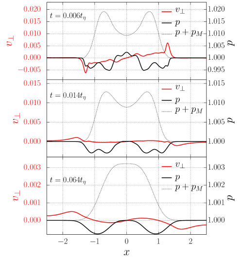
Figure 6: Fluid velocity $v_{\perp}$ (red) pressure $p$ (black), and total pressure $p+p_{M}$ along the $x$-axis at three different times corresponding to the second, third, and fifth top panel in figure 2. The resistivity of this run was $\eta=2\times 10^{-4}$ and $\imath_{0}^{*}=3$. During the initial reconfiguration, the pressure profile is irregular, but the total pressure is smooth. In the last panel the equilibrium has reached the state where the magnetic axis is located at the minimum in pressure. The flow profile shows a net flow towards the magnetic axis which is similar to Pfirsch-Schlüter diffusion.

Whilst the fluid flow slowly penetrates the magnetic structure, the magnetic energy in the structure is decreasing. The decrease of total magnetic energy for the simulations with $\imath_{0}^{*}=3$ and $B_{0}=0.05$ is shown in figure 7.

One important result to note is that the magnetic field strength decays fast compared to the resistive decay time $t_{\eta}$, whereas in general the magnetic field strength is expected to evolve as $\langle|\bm{B}|\rangle\sim\langle B_{0}\rangle e^{-t/t_{\eta}}$. Here the magnetic energy has already decreased an order of magnitude in only $0.1t_{\eta}$. This is because the resistive losses are not the only mechanism through which the magnetic field is lowered: During the evolution the entire configuration also expands. Even with zero resistivity such an expansion leads to a lowering of the magnetic field strength. This can be seen as follows: since it is the flux through a co-moving surface that is conserved, and if that surface expands, the magnetic field strength lowers. This effect can also be seen in the zero resistance simulations presented in (Smiet et al., 2016).

figure 7 also shows the evolution of magnetic helicity, which decreases at a slower rate than the magnetic energy. The slower decay of helicity can be seen as the result of the expansion, as the structure evolves with a self-similar shape. The magnetic energy is the integral of $(\nabla\times\bm{A})\cdot(\nabla\times\bm{A})$, whereas the integrand of the helicity integral, $\bm{A}\cdot(\nabla\times\bm{A})$, involves one less spatial derivation. For a similar structure of a larger size, the magnetic helicity is thus larger. Note that we evolve these structures on a timescale larger than the timescales on which the helicity can be considered conserved, and that our initial condition is intentionally very regular. Therefore the localized reconnections which transform helicty between linking, writhe, and twist, which reconfigure the magnetic topology whilst leaving helicity mostly unchanged in turbulent Woltjer-Taylor type relaxation are absent in these runs. See (Smiet et al., 2015) for simulations where this equilibrium is achieved through this more chaotic reconnection.

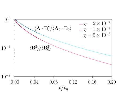
Figure 7: Decay of magnetic energy and decay of total helicity versus time for the runs with $\imath_{0}^{*}=3$ and $B_{0}=0.05$ for different values of resistivity $\eta$.

Finally we look at the change of rotational transform in time, and how it depends on the initial value for the rotational transform. The results are shown in figure 8. From the asymptotic behaviour in the log-log plot we can see that the rotational transform decays according to a power law instead of exponentially. The characteristic exponent of this decay is different for runs with different $\imath_{0}^{*}$. The rotational transform between $t_{\eta}=0.05$ and $t_{\eta}=0.1$ is fitted with a power law $\imath^{*}(t)=a{t_{\eta}}^{-b}$ and a characteristic exponent of $b=0.664$ is found for the run with $\imath_{0}^{*}=10$ and $b=0.48$ for the run with $\imath_{0}^{*}=3$. Guides are drawn in figure 8 showing $t_{\eta}^{-2/3}$ and $t_{\eta}^{-1/2}$ decay.

The lowering rotational transform is caused by the poloidal field decreasing faster than the toroidal field. This is another indication that the lowering of field strength is primarily caused by the expansion of the structure caused by field line slip and not necessarily by resistive decay. With resistive decay we indicate the exponential decay with characteristic decay time $t_{\eta}$ caused by resistivity on a static field configuration, solutions of equation (16) with $\mbox{\boldmath$v$}{}=0$. Decay brought on by field line slip is caused by the non-zero Pfirsch-Schlüter flow, or conversely the motion of the field lines against the plasma. This causes the term $v$ to be non-zero and the term $\nabla^{2}\bm{A}$ to decrease (through expansion the gradients get smaller) in equation (16), and thus the change in magnetic field strength can be fast compared to the resistive decay time.

As the structure expands the poloidal field strength is lowered by expansion in the horizontal plane, as it is the poloidal flux passing through the circle defined by the magnetic axis which is conserved. The increase in area through which this flux passes is proportional to $(R^{*})^{2}$. The lowering of the toroidal field meanwhile is governed by the change in area of the poloidal cross-section of the flux tube. Expansion in this plane is constrained to the positive $R$-direction and as such the area should go approximately linear in $R^{*}$. This constrained expansion is attested by the D-shaped magnetic surfaces seen in the top row of figure 2. Even though this explanation is quite qualitative and does not take into account the shape of the surfaces and the distribution of magnetic flux, it does explain why the rotational transform lowers according to a power law. Furthermore, the difference between poloidal and toroidal expansion correctly predicts a characteristic exponent of around $-1/2$.

It should be noted that the decay in rotational transform is fast compared to the increase of the major radius of the structure; the rotational transform changes by a factor of three in the time $R^{*}$ only changes a few percent. This is important when considering this equilibrium as a model for magnetic clouds.

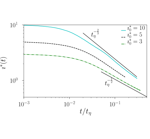
Figure 8: Time dependence of the rotational transform for different values of $\imath_{0}^{*}$. After the initial period where the magnetic structure re-organizes on an Alfvénic timescale, the rotational transform decays following a power law with characteristic exponent between $-2/3$ and $-1/2$.

6 Relation to magnetic clouds

The presented simulations of axisymmetric equilibria are more idealized than the situation encountered in the solar wind. As noted in the introduction, the plasma $\beta$ in the solar wind is around 1, and a signature of a magnetic cloud is that the $\beta$ drops below 1 (Zurbuchen & Richardson, 2006). In these simulations, the initial $\beta$ (taking the magnetic field strength and pressure on the axis) is around 25 when $B_{0}=0.05$ and 1.65 when $B_{0}=0.2$. However, as can be seen from figure 5, when rescaled to resistive time the evolution of the fields is near identical. Simulations (not presented in this paper) have been performed at $\beta$ down to 0.7 which show the same evolution, but this is not a lower limit. The simulations show the set-up of a toroidal equilibrium against a background plasma with lower field strength, similar to the situation encountered in the solar wind.

In the solar wind the Alfvén speed and the sound speed are the same order of magnitude with $v_{s}=37$ km $\rm{s}^{-1}$ and $v_{A}=47$km $\rm{s}^{-1}$ (Goedbloed & Poedts, 2004). Assuming a magnetic cloud size of approximately $10^{6}$ km (1 day passage for a probe travelling at 15 km $\rm{s}^{-1}$), the Alfvénic transit time is around 7 hours, so one dozen to several dozen Alfvén transit times pass between coronal mass ejection and observation, a similar regime as is probed in the simulation. The magnetic Prandtl number (ratio of kinematic viscosity to magnetic diffusivity) for a hot thin plasma such as the interplanetary solar wind is much higher than unity; $\sim 10^{14}$ (see Brandenburg & Subramanian (2005)). The plasma in the solar wind is thus in a regime here the viscous forces act faster than the resistivity to allow for a similar self-organizing process as observed in the simulations. One major difference is that $t_{\eta}$ for a magnetic cloud is about $10^{9}$ years, much longer than the months for which a cloud can be observed before it leaves the solar system. When the cloud is just ejected, $R_{\rm char}$ is smaller and reconnection can occur (it must to trigger the ejection). Furthermore the more chaotic solar wind allows for small-scale reconnection events which increase the effective reconnection rate. Nevertheless, the extent to which the rotational transform changes must be much smaller than the full evolution presented in this paper.

There are several models for magnetic clouds discussed in literature, see for example  (Burlaga, 1991) for an overview. One of the more common approaches is to model a magnetic cloud as a long flux rope extending from, and still magnetically connected, to the surface of the sun. Nevertheless there are several models that consider magnetic clouds as localized magnetic excitations within the solar wind, with their magnetic field generated by internal currents.

Kumar and Rust describe a model for a magnetic cloud as an isolated, net current carrying toroidal flux ring (Kumar & Rust, 1996). The magnetic field inside the ring is based on the force free Lundquist solution valid for an infinite cylinder (Lundquist, 1950). As they themselves note, this cannot be an exact description, as the toroidal geometry necessitates the existence of a hoop force such as described in (Garren & Chen, 1994). In this model the plasma current is zero outside of the toroid, but the net current through the toroid is non-zero such that it generates a force-free field in the surrounding plasma.

There are several differences between Kumar and Rust’s model and a magnetic cloud as a self-organized structure we describe. Firstly the magnetic field in their model is force free. Such a field is not possible, as they note themselves because a current ring will always experience a hoop force. The rotational transform profile in their model is also very different. In Lundquist solutions the axial and tangential fields (which, when the cylinder is translated to a torus, correspond to the toroidal and poloidal directions respectively) are given by Bessel functions. As such the rotational transform profile changes significantly from the magnetic axis to the edge (Bellan, 2000). The magnetic field outside the ring is purely toroidal, which implies that the rotational transform goes to infinity. Even though their model resembles the configuration we describe superficially, the rotational transform profile is drastically different. Our simulations show that the profile quickly flattens.

Another magnetic cloud model which resembles the configurations we observe is the flare-generated spheromak model by Ivanov and Harshiladze (Ivanov & Harshiladze, 1985) and further explored by Vandas et al. (Vandas et al., 1992). They describe the clouds using the spherical force free solution of Chandrasekhar and Kendall (Chandrasekhar & Kendall, 1957). The magnetic topology in this solution also consists of field lines lying on nested toroidal surfaces. In this model the rotational transform profile of these force free solutions is also non-constant.

The resistive decay time for a structure with the characteristic length scale that is reasonable for magnetic clouds, $R_{\rm char}=10^{6}{\rm km}$, is about $1.7\times 10^{9}$ years (Goedbloed & Poedts, 2004), so change in the rotational transform due to resistive processes is expected to be small. The process leading to the formation of the self-organized localized equilibrium however takes place on a much faster timescale. Note that not just the Alfvénic oscillation towards equilibrium is fast; as seen in figure 2 much of the change in rotational transform towards equilibrium has already occurred at $0.006t_{\eta}$. This change, though fast, scales with resistivity. If the resistivity is many orders of magnitude lower, as in the solar wind, this change in rotational transform can be expected to be much less rapid, and the cloud will still carry much of the topology it organized into when it was ejected. The evolution of the magnetic structure, after it is generated, can therefore be considered to be approximately ideal, as is also assumed in the model by Ivanov and Harshiladze and the model by Kumar and Rust.

Because the structure we describe does not rely on the assumption of force free fields, an assumption that is not warranted in the $\beta\sim 1$ solar wind plasma, we speculate that the magnetic structures described in this paper are a more realistic model for localized magnetic clouds than the two others described above.

7 Conclusions

In this paper we have shown how a self-organizing equilibrium evolves on a resistive time scale. In agreement with our previous studies we find that the initially twisted flux tube reconfigures on an Alfvénic timescale into an axisymmetric Grad-Shafranov equilibrium characterized by a lowered pressure on the magnetic axis.

In this paper we have described how the configuration evolves subsequently; the major radius $R^{*}$ grows, and the rotational transform on the magnetic axis $\imath^{*}(t)$ lowers. The rotational transform profile, which initially had a high positive curvature, quickly evolves to a almost flat and slightly negatively curved profile.

With the exception of the initial reconfiguration which proceeds on an Alfvénic timescale, the evolution is rather independent on the resistivity when scaled to a resistive timescale. The growth of the structure can be understood as a Pfirsch-Schlüter-type slip of the field lines against the plasma fluid background, or conversely the fluid slip against the field.

It is because of this growth of the structure that the magnetic field strength decays faster than the resistive timescale. It is also this growth which allows the poloidal field to decay faster than the toroidal field. We have also given a simple geometrical argument that explains why the decay of the rotational transform behaves as a power law with characteristic exponent of the order of $1/2$.

In this study we have limited ourselves to isothermal (constant resistivity) MHD evolution. The inclusion of temperature would result in a spatial variation of the Spitzer resistivity, which would quantitatively change the exact evolution, but the general aspects of the equilibrium and its evolution are underlied by geometrical principles and would remain unchanged. It is an interesting question whether the generation of a flat rotational transform profile would remain robust under these conditions

These results could help make predictions for the evolution of self-organized magnetic equilibria in nature. In this paper we relate this structure to magnetic clouds. Other applications for this model include AGN ejecta (Braithwaite, 2010), and one could possibly devise a scheme for pulsed nuclear fusion power generation in which the plasma is confined in such a magnetic structure, embedded in an extremely high fluid pressure environment. When devising such a scheme it should be important to note that the decay time of the magnetic field strength proceeds on a timescale much faster than the resistive decay time, and as such that the ‘confinement’ is a very transient phenomenon.

8 Acknowledgements

We wish to thank the anonymous referees for their careful review of our article.

This work is part of the Rubicon programme with project number 680-50-1532, which is (partly) financed by the Netherlands Organization for Scientific Research (NWO).

DIFFER is part of the Netherlands Organisation for Scientific Research (NWO).

Notice: This manuscript is based upon work supported by the U.S. Department of Energy, Office of Science, Office of Fusion Energy Sciences, and has been authored by Princeton University under Contract Number DE-AC02-09CH11466 with the U.S. Department of Energy. The publisher, by accepting the article for publication acknowledges, that the United States Government retains a non-exclusive, paid-up, irrevocable, world-wide license to publish or reproduce the published form of this manuscript, or allow others to do so, for United States Government purposes.

References

- Alfvén (1943) Alfvén, H. 1943 On the existence of electromagnetic-hydrodynamic waves. Arkiv for Astronomi 29, 1–7.
- Arnol’d (1986) Arnol’d, V. I. 1986 The asymptotic hopf invariant and its applications. Sel. Math. Sov 5 (4), 327.
- Arrayás & Trueba (2014) Arrayás, M. & Trueba, J. L. 2014 A class of non-null toroidal electromagnetic fields and its relation to the model of electromagnetic knots. Journal of Physics A: Mathematical and Theoretical 48 (2), 025203.
- Batchelor (1950) Batchelor, G. K. 1950 On the Spontaneous Magnetic Field in a Conducting Liquid in Turbulent Motion. Royal Society of London Proceedings Series A 201 (1066), 405–416.
- Bellan (2000) Bellan, P. M. 2000 Spheromaks: a practical application of magnetohydrodynamic dynamos and plasma self-organization. World Scientific.
- Berger & Field (1984) Berger, M. A. & Field, G. B. 1984 The topological properties of magnetic helicity. Journal of Fluid Mechanics 147, 133–148.
- Braithwaite (2010) Braithwaite, J. 2010 Magnetohydrodynamic relaxation of agn ejecta: radio bubbles in the intracluster medium. Monthly Notices of the Royal Astronomical Society 406 (2), 705–719.
- Brandenburg & Dobler (2002) Brandenburg, A. & Dobler, W. 2002 Hydromagnetic turbulence in computer simulations. Computer Physics Communications 147 (1-2), 471–475.
- Brandenburg & Subramanian (2005) Brandenburg, A. & Subramanian, K. 2005 Astrophysical magnetic fields and nonlinear dynamo theory. Physics Reports 417 (1-4), 1–209.
- Burlaga (1991) Burlaga, L. F. 1991 Magnetic clouds. In Physics of the Inner Heliosphere II, pp. 1–22. Springer.
- Candelaresi & Brandenburg (2011) Candelaresi, S. & Brandenburg, A. 2011 Decay of helical and nonhelical magnetic knots. Physical Review E 84 (1), 016406.
- Chandrasekhar & Kendall (1957) Chandrasekhar, S. & Kendall, P. 1957 On force-free magnetic fields. The Astrophysical Journal 126, 457.
- Del Sordo et al. (2010) Del Sordo, F., Candelaresi, S. & Brandenburg, A. 2010 Magnetic-field decay of three interlocked flux rings with zero linking number. Physical Review E 81 (3), 036401.
- Finkelstein & Weil (1978) Finkelstein, D. & Weil, D. 1978 Magnetohydrodynamic kinks in astrophysics. International Journal of Theoretical Physics 17 (3), 201–217.
- Garren & Chen (1994) Garren, D. A. & Chen, J. 1994 Lorentz self-forces on curved current loops. Physics of plasmas 1 (10), 3425–3436.
- Goedbloed et al. (2010) Goedbloed, J. P., Keppens, R. & Poedts, S. 2010 Advanced magnetohydrodynamics: with applications to laboratory and astrophysical plasmas. Cambridge University Press.
- Goedbloed & Poedts (2004) Goedbloed, J. P. & Poedts, S. 2004 Principles of magnetohydrodynamics: with applications to laboratory and astrophysical plasmas. Cambridge university press.
- Haugen et al. (2004) Haugen, N. E. L., Brandenburg, A. & Dobler, W. 2004 Simulations of nonhelical hydromagnetic turbulence. Physical Review E 70 (1), 016308.
- Hopf (1931) Hopf, H. 1931 Über die Abbildungen der dreidimensionalen Sphäre auf die Kugelfläche. Math. Ann. 104 (1), 637–665.
- Ivanov & Harshiladze (1985) Ivanov, K. & Harshiladze, A. 1985 Interplanetary hydromagnetic clouds as flare-generated spheromaks. Solar physics 98 (2), 379–386.
- Johansen et al. (2007) Johansen, A., Oishi, J. S., Mac Low, M.-M., Klahr, H., Henning, T. & Youdin, A. 2007 Rapid planetesimal formation in turbulent circumstellar disks. Nature 448 (7157), 1022.
- Kulsrud (2011) Kulsrud, R. M. 2011 Intuitive approach to magnetic reconnection. Physics of Plasmas (1994-present) 18 (11), 111201.
- Kumar & Rust (1996) Kumar, A. & Rust, D. 1996 Interplanetary magnetic clouds, helicity conservation, and current-core flux-ropes. Journal of Geophysical Research: Space Physics 101 (A7), 15667–15684.
- Lundquist (1950) Lundquist, S. 1950 Magneto-hydrostatic fields. Arkiv for fysik 2 (4), 361–365.
- Moffatt (1969) Moffatt, H. K. 1969 The degree of knottedness of tangled vortex lines. Journal of Fluid Mechanics 35 (1), 117–129.
- Priest & Forbes (2000) Priest, E. R. & Forbes, T. G. 2000 Magnetic reconnection: MHD theory and applications. Cambridge University Press.
- Raghav & Kule (2018) Raghav, A. N. & Kule, A. 2018 The first in situ observation of torsional alfvén waves during the interaction of large-scale magnetic clouds. Monthly Notices of the Royal Astronomical Society: Letters 476 (1), L6–L9.
- Shafranov (1966) Shafranov, V. 1966 Plasma equilibrium in a magnetic field. Reviews of Plasma Physics 2, 103.
- Smiet et al. (2015) Smiet, C., Candelaresi, S., Thompson, A., Swearngin, J., Dalhuisen, J. & Bouwmeester, D. 2015 Self-organizing knotted magnetic structures in plasma. Physical review letters 115 (9), 095001.
- Smiet et al. (2016) Smiet, C. B., Candelaresi, S. & Bouwmeester, D. 2016 Ideal relaxation of the hopf fibration. arXiv preprint arXiv:1610.04719 .
- Taylor (1974) Taylor, J. 1974 Relaxation of toroidal plasma and generation of reverse magnetic fields. Phys. Rev. Lett. 33 (19), 1139–1141.
- Taylor (1986) Taylor, J. 1986 Relaxation and magnetic reconnection in plasmas. Reviews of Modern Physics 58 (3), 741.
- Vandas et al. (1992) Vandas, M., Fischer, S., Pelant, P. & Geranios, A. 1992 Magnetic clouds-comparison between spacecraft measurements and theoretical magnetic force-free solutions. In Solar Wind Seven Colloquium, , vol. 1, pp. 671–674.
- Wesson & Campbell (2011) Wesson, J. & Campbell, D. J. 2011 Tokamaks, , vol. 149. Oxford University Press.
- Woltjer (1958) Woltjer, L. 1958 A theorem on force-free magnetic fields. Proceedings of the National Academy of Sciences 44 (6), 489–491.
- Zurbuchen & Richardson (2006) Zurbuchen, T. H. & Richardson, I. G. 2006 In-situ solar wind and magnetic field signatures of interplanetary coronal mass ejections. In Coronal Mass Ejections, pp. 31–43. Springer.