Computational Bounds For Photonic Design

Abstract

Physical design problems, such as photonic inverse design, are typically solved using local optimization methods. These methods often produce what appear to be good or very good designs when compared to classical design methods, but it is not known how far from optimal such designs really are. We address this issue by developing methods for computing a bound on the true optimal value of a physical design problem; physical designs with objective smaller than our bound are impossible to achieve. Our bound is based on Lagrange duality and exploits the special mathematical structure of these physical design problems. For a multi-mode 2D Helmholtz resonator, numerical examples show that the bounds we compute are often close to the objective values obtained using local optimization methods, which reveals that the designs are not only good, but in fact nearly optimal. Our computational bounding method also produces, as a by-product, a reasonable starting point for local optimization methods.

1 Introduction

Computer-aided design of physical systems is growing rapidly in several fields, including photonics [MLP⁺18] (where it is known as inverse design), horn design [NUS⁺10], and mechanical design (aerospace, structures) [HG12]. These design methods formulate the physical design problem as a constrained nonconvex optimization problem, and then use local optimization to attempt to solve the problem. Commonly used methods include gradient descent, with adjoint-based evaluations of the gradient [LKBMY13], methods that alternate optimizing over the structure and over the response [LV10], and the alternating directions method of multipliers (ADMM) [LV13], among others. These methods can be very effective, in the sense of producing what appear to be very good physical designs, for example when compared to classical design approaches.

Because they are local optimization methods, they do not guarantee that a globally optimal design is found, nor do we know how far from optimal the resulting design is. This paper addresses the question of how far a physical design is from globally optimal by computing a lower bound on the optimal objective value of the optimization problem. A lower bound on the objective value can be interpreted as an impossibility result since it asserts that no physical design can have a lower objective than a number we compute.

Our bound is similar in spirit to analytical lower bounds, which give lower bounds as simple formulas in terms of gross quantities like temperature and wavelength, based on very simplified models and objectives, e.g., the Reynolds number [Pur77], the Carnot efficiency limit [Fer36, §3.8], or the optical diffraction limit [BW13, §8.6]. There has been some additional work in bounding some other quantities and figures of merit for optical systems, including the local density of states [MPR⁺16, SFJM18] for different types of materials, via fundamental physical principles. In contrast, our method computes a (numerical) lower bound for the optimization objective for each design problem.

In this paper, we derive a parametrized family of lower bounds on the optimal objective for a class of physical design problems, using Lagrange duality. We can optimize over the parameter, to obtain the best (largest) lower bound, by solving the Lagrange dual problem—which is convex even though the original design problem is not. We illustrate our lower bound on a two-dimensional multi-mode resonator. Our lower bound is close to the objective obtained by a design using ADMM, which shows that the design, and indeed our lower bound, are both very close to the global optimum.

2 Physical design

2.1 Physical design problem

In physical design, we design a structure so that the field, under a given excitation, is close to some desired or target field. We parametrize the structure using a vector $\theta$, and we denote the field by the vector $z$. In photonic design, for example, we choose the index of refraction at each rectangle on a grid, within limits, to achieve or get close to a desired electromagnetic field.

We can express this as the following optimization problem:

$$\begin{array}[]{ll}\mbox{minimize}&\frac{1}{2}\left\|{W(z-\hat{z})}\right\|_{2}^{2}\\ \mbox{subject to}&(A+\mathop{\bf diag}(\theta))z=b\\ &0\leq\theta\leq\theta^{\mathrm{max}},\end{array}$$ (1)

with variables $z\in{\mbox{\bf R}}^{n}$ (the field) and $\theta\in{\mbox{\bf R}}^{n}$, which describes the physical design. The data are the weight matrix $W\in{\mbox{\bf R}}^{n\times n}$, which is diagonal with positive diagonal entries, the desired or target field $\hat{z}\in{\mbox{\bf R}}^{n}$, the matrix $A\in{\mbox{\bf R}}^{n\times n}$, the excitation vector $b\in{\mbox{\bf R}}^{n}$, and the vector $\theta^{\mathrm{max}}$ of limits on the physical design parameter $\theta$. The constraint equation $(A+\mathop{\bf diag}(\theta))z=b$ encodes the physics of the problem. We let $p^{\star}$ denote the optimal value of (1).

We can handle the case when the lower limit on the physical parameter is nonzero, for example, $\theta^{\mathrm{min}}\leq\theta\leq\theta^{\mathrm{max}}$. We do this by replacing the lower limit by $0$, the upper limit by $\theta^{\mathrm{max}}-\theta^{\mathrm{min}}$, and replacing $A$ with $A+\mathop{\bf diag}(\theta^{\mathrm{min}})$. Additionally, the construction extends easily to the case where the field $z$, the matrix $A$, and the excitation $b$ have complex entries.

When the coefficient matrix in the physics equation $(A+\mathop{\bf diag}(\theta))z=b$ is nonsingular, there is a unique field, $z=(A+\mathop{\bf diag}(\theta))^{-1}b$. In some applications, however, the coefficient matrix is singular, and there is either no field that satisfies the equations, or many. In the former case, we take the objective to be $+\infty$. In the latter case, the set of solutions is an affine set and simple least squares can be used to find the field that satisfies the physics equation and minimizes the objective.

An important special case occurs when we seek a mode (eigenvector) of a system that is close to $\hat{z}$. To do this we take $b=0$ and subtract $\lambda I$ from the coefficient matrix, where $\lambda$ is the required eigenvalue. We can handle the case of unspecified eigenvalues by a simple extension described later in problem (14), where $\lambda$ also becomes a design variable, subject to a lower and upper bound.

In the problem (1), the physical design parameters enter in a very specific way: as the diagonal entries of the coefficient matrix of the physics equation. Many physics equations have this form for a suitable definition of the field $z$ and parameter $\theta$, including the time-independent Schödinger equation, Helmholtz’s equation, the heat equation, and Maxwell’s equations in one dimension. (Maxwell’s equations in two and three dimensions are included in this formalism via the simple extension given in problem (13).)

Boolean physical design problem.

A variation on the problem (1) replaces the physical parameter constraint $0\leq\theta_{j}\leq\theta^{\mathrm{max}}_{j}$ with the constraint $\theta_{j}\in\{0,\theta^{\mathrm{max}}_{j}\}$, which limits each physical parameter value to only two possible values. (This occurs when we are choosing between two materials, such as silicon or air, in each of the patches in the structure we are designing.) We refer to this modified problem as the Boolean physical design problem, as opposed to the continuous physical design problem (1). It is clear that the optimal value of the Boolean physical design is no smaller than $p^{\star}$, the optimal value of the continuous physical design problem.

2.2 Approximate solutions

The problem (1) is not convex and generally hard to solve exactly [BV04]. It is, however, bi-convex, since it is convex in $z$ when $\theta$ is fixed, and convex in $\theta$ when $z$ is fixed. Using variations on this observation, researchers have developed a number of methods for approximately solving (1) via heuristic means, such as alternating optimization over $z$ and $\theta$ on the augmented Lagrangian of this problem [LV13]. Other heuristics can be used to find approximate solutions of the Boolean physical design problem. These methods produce what appear to be very good physical designs when compared to previous hand-crafted designs or classical designs.

2.3 Performance bounds

Since the approximate solution methods used are local and therefore heuristic, the question arises: how far are these approximate designs from an optimal design? In other words, how far is the objective found by these methods from $p^{\star}$? Suppose, for example, that a heuristic method finds a design with objective value 13.1. We do not know what the optimal objective $p^{\star}$ is, other than $p^{\star}\leq 13.1$. Does there exist a design with objective value 10? Or 5? Or are these values of the objective impossible, i.e., smaller than $p^{\star}$?

The method described in this paper aims to answer this question. Specifically, we will compute a provable lower bound $L$ on the optimal objective value $p^{\star}$ of (1). In our example above, our method might compute the lower bound value $L=12.5$. This means that no design can ever achieve an objective value smaller than 12.5. It also means that a design with an objective value of 13.1 is not too far from optimal, since we would know that $L=12.5\leq p^{\star}\leq 13.1$.

A lower bound $L$ on $p^{\star}$ can be interpreted as an impossibility result, since it tells us that it is impossible for a physical design to achieve an objective value less than $L$. We can also interpret $L$ as a performance bound. The lower bound $L$ does not tell us what $p^{\star}$ is; it just gives a lower limit on what it can be. (An upper limit $U$ can be found by using any heuristic method, as the final objective value attained.)

We note that the lower bound $L$ we find on $p^{\star}$ also serves as a lower bound on the optimal value of the Boolean physical design problem, since its optimal value is larger than or equal to $p^{\star}$.

3 Performance bounds via Lagrange duality

In this section, we explain our lower bound method.

3.1 Lagrangian duality

We first rewrite (1) as

$$\begin{array}[]{ll}\mbox{minimize}&\frac{1}{2}\left\|{W(z-\hat{z})}\right\|_{2}^{2}+I(\theta)\\ \mbox{subject to}&(A+\mathop{\bf diag}(\theta))z=b,\end{array}$$ (2)

where $I$ is an indicator function, i.e., $I(\theta)=0$ when $0\leq\theta\leq\theta^{\mathrm{max}}$ and $+\infty$ otherwise. The Lagrangian of this problem is

$$\mathcal{L}(z,\theta,\nu)=\frac{1}{2}\left\|{W(z-\hat{z})}\right\|_{2}^{2}+I(\theta)+\nu^{T}((A+\mathop{\bf diag}(\theta))z-b),$$ (3)

where $\nu\in{\mbox{\bf R}}^{n}$ is a dual variable. The Lagrange dual function is

$$g(\nu)=\inf_{\theta,z}\mathcal{L}(z,\theta,\nu).$$

(See [BV04, Chapter 5].) It is a basic and easily proved fact that for any $\nu$, we have $g(\nu)\leq p^{\star}$ (see [BV04, §5.1.3]). In other words, $g(\nu)$ is a lower bound on $p^{\star}$. While $g(\nu)$ always gives a lower bound on $p^{\star}$, the challenge for nonconvex problems such as (1) is to evaluate $g(\nu)$. We will see now that this can be done for our problem (1).

3.2 Evaluating the dual function

To evaluate $g(\nu)$ we must minimize $\mathcal{L}(z,\theta,\nu)$ over $z$ and $\theta$. Since for each $\theta$, $\mathcal{L}(z,\theta,\nu)$ is convex quadratic in $z$, we can analytically carry out the minimization over $z$. We have

$$g(\nu) =\inf_{\theta}\inf_{z}\mathcal{L}(z,\theta,\nu)$$

$$=\inf_{\theta}\left(-\frac{1}{2}\left\|{W^{-1}((A+\mathop{\bf diag}(\theta))^{T}\nu-W^{2}\hat{z})}\right\|_{2}^{2}-\nu^{T}b+\frac{1}{2}\left\|{W\hat{z}}\right\|_{2}^{2}+I(\theta)\right)$$

$$=\inf_{0\leq\theta\leq\theta^{\mathrm{max}}}-\frac{1}{2}\left\|{W^{-1}((A+\mathop{\bf diag}(\theta))^{T}\nu-W^{2}\hat{z})}\right\|_{2}^{2}-\nu^{T}b+\frac{1}{2}\left\|{W\hat{z}}\right\|_{2}^{2}.$$ (4)

We can see that this is true since the minimizer of the only terms depending on $z$,

$$\mathop{\rm argmin}_{z}\left(\frac{1}{2}\left\|{W(z-\hat{z})}\right\|_{2}^{2}+\nu^{T}(A+\mathop{\bf diag}(\theta))z\right),$$

can be found by taking the gradient and setting it to zero (which is necessary and sufficient by convexity and differentiability). This gives that the minimizing $z$ is

$$z=\hat{z}-W^{-2}(A+\mathop{\bf diag}(\theta))\nu,$$ (5)

which yields (4) when plugged in.

The expression in (4) is separable over each $\theta_{i}$; it can be rewritten as

$$g(\nu) =\inf_{0\leq\theta\leq\theta^{\mathrm{max}}}-\frac{1}{2}\sum_{j=1}^{n}W_{jj}^{-2}\left((A^{T}\nu)_{j}+\nu_{j}\theta_{j}-W^{2}_{jj}\hat{z}_{j}\right)^{2}-\nu^{T}b+\frac{1}{2}\left\|{W\hat{z}}\right\|_{2}^{2}$$

$$=\sum_{j=1}^{n}\left(\inf_{0\leq\theta_{j}\leq\theta^{\mathrm{max}}_{j}}-\frac{1}{2}W_{jj}^{-2}\left((A^{T}\nu)_{j}+\nu_{j}\theta_{j}-W^{2}_{jj}\hat{z}_{j}\right)^{2}\right)-\nu^{T}b+\frac{1}{2}\left\|{W\hat{z}}\right\|_{2}^{2}$$

$$=-\frac{1}{2}\sum_{j=1}^{n}W_{jj}^{-2}\max\left\{\left(a^{T}_{j}\nu-W^{2}_{jj}\hat{z}_{j}\right)^{2},\left(a^{T}_{j}\nu+\nu_{j}\theta^{\mathrm{max}}_{j}-W^{2}_{jj}\hat{z}_{j}\right)^{2}\right\}-\nu^{T}b+\frac{1}{2}\left\|{W\hat{z}}\right\|_{2}^{2},$$ (6)

where $a_{j}$ is the $j$th column of $A$. In the last line, we use the basic fact that a scalar convex quadratic function achieves its maximum over an interval at the interval’s boundary.

With this simple expression for the dual function, we can now generate lower bounds on $p^{\star}$, by simply evaluating it for any $\nu$. We note that $g$ is also the dual function of the Boolean physical design problem.

3.3 Dual optimization problem

It is natural to seek the best or largest lower bound on $p^{\star}$, by choosing $\nu$ that maximizes our lower bound. This leads to the dual problem (see [BV04, §5.2]),

$$\begin{array}[]{ll}\mbox{maximize}&g(\nu),\end{array}$$

with variable $\nu$. We denote the optimal value as $d^{\star}$, which is the best lower bound on $p^{\star}$ that can be found from the Lagrange dual function. The dual problem is always a convex optimization problem (see [BV04, §5.1.2]); to effectively use it, we need a way to tractably maximize $g$, which we have in our case, since the dual problem can be expressed as the convex quadratically-constrained quadratic program (QCQP)

$$\begin{array}[]{ll}\mbox{maximize}&-(1/2)\mathbf{1}^{T}t-\nu^{T}b+(1/2)\left\|{W\hat{z}}\right\|_{2}^{2}\\ \mbox{subject to}&t_{j}\geq W_{jj}^{-2}\left(a_{j}^{T}\nu-W_{jj}^{2}\hat{z}_{j}\right)^{2},~{}~{}j=1,\dots,n\\ &t_{j}\geq W_{jj}^{-2}\left(a_{j}^{T}\nu+\nu_{j}\theta^{\mathrm{max}}_{j}-W_{jj}^{2}\hat{z}_{j}\right)^{2},~{}~{}j=1,\dots,n,\end{array}$$ (7)

with variables $t$ and $\nu$. This problem is easily solved and its optimal value, $d^{\star}$, is a lower bound on $p^{\star}$.

The dual optimization problem (7) can be solved several ways, including via ADMM (which can exploit the fact that all subproblems are quadratic; see [BPC⁺11a]), interior point methods (see [BV04, §11.1]), or by rewriting it as a second-order cone program (SOCP) (see [LVBL98]; this can also be done automatically by modeling languages such as CVXPY [AVDB18]) and then using one of the many available SOCP solvers, such as SCS [OCPB16a, OCPB16b], ECOS [DCB13], or Gurobi [GO18]. We also note that the dual problem does not have to be perfectly solved; we get a lower bound for any value of the dual variable $\nu$.

In this paper, we used the Gurobi solver to solve a (sparse) program with $n=63001$, which took approximately 8 minutes to solve on a two-core Intel Core i5 machine with 8GB of RAM. By further exploiting the structure of the problem, giving good initializations, or by using less accurate methods when small tolerances are not required, it is likely that these problems could be solved even more quickly, for larger systems.

3.4 Initializations via Lagrange dual

The solution of the Lagrange dual problem can be used to suggest starting points in a heuristic or local method for approximately solving (1).

Initial structure.

Let $\nu^{\star}$ be a solution of the dual problem (7). We can take as initial structure $\theta^{0}$ which minimizes (4), i.e.,

$$\theta^{0}_{j}\in\mathop{\rm argmax}_{\theta_{j}\in\{0,\,\theta^{\mathrm{max}}_{j}\}}\left(a_{j}^{T}\nu^{\star}+\nu_{j}^{\star}\theta_{j}-W_{jj}^{2}\hat{z}_{j}\right)^{2}.$$

This choice of initial structure is feasible for (1) and, in fact, is feasible for the Boolean physical design problem as well.

Initial field.

One way to obtain an initial field is to simply solve the physics equation for $\theta^{0}$, when the physics coefficient matrix is nonsingular. When it is singular, but the physics equation is solvable, we compute $z$ as the field that minimizes the objective, subject to the physics equation. This gives a feasible field, but in some cases the resulting point is not very useful. For example when $b=0$, and the coefficient matrix is nonsingular, we obtain $z^{0}=0$.

Another possibility is to find the minimizer of the Lagrangian with the given structure and an optimal dual variable value, i.e.,

$$z^{0}=\mathop{\rm argmin}_{z}\mathcal{L}(\theta^{0},z,\nu^{\star}).$$

The value is already given in (5):

$$z^{0}=\hat{z}-W^{-2}\left(A+\mathop{\bf diag}(\theta^{0})\right)^{T}\nu^{\star}.$$

This initial field is not feasible, i.e., it does not satisfy the physics equation, but it seems to be a very good initial choice for heuristic algorithms.

4 Multi-scenario design

In this section we mention an extension of our basic problem (1), in which we wish to design one physical structure that gives reasonable performance in $N$ different scenarios. The scenarios can represent different operating temperatures, different frequencies, or different modes of excitation.

We will index the scenarios by the superscript $i$, with $i=1,\ldots,N$. Each scenario can have a different weight matrix $W^{i}$, a different target field $\hat{z}^{i}$, a different physics matrix $A^{i}$, and a different excitation $b^{i}$. We have only one physical design variable $\theta$, and $N$ different field responses, $z^{i}$, $i=1,\ldots,N$. We take as our overall objective the sum (or average) of the objectives under the scenarios. This leads to the problem

$$\begin{array}[]{ll}\mbox{minimize}&\frac{1}{2}\sum_{i=1}^{N}\left\|{W^{i}(z^{i}-\hat{z}^{i})}\right\|_{2}^{2}\\ \mbox{subject to}&(A^{i}+\mathop{\bf diag}(\theta))z^{i}=b^{i},~{}~{}i=1,\dots,N\\ &0\leq\theta\leq\theta^{\mathrm{max}},\end{array}$$ (8)

with variables $\theta$ (the structure) and $z^{i}$ (the fields under the $N$ different scenarios).

Our bounding method easily generalizes to this multi-scenario physical design problem.

Dual optimization problem.

As before, define $a^{i}_{j}$ to be the $j$th column of $A^{i}$ and allow $\nu^{i}$ to be the Lagrange multiplier for the $i$th constraint, then the new dual problem is,

$$\begin{array}[]{ll}\mbox{maximize}&-(1/2)\mathbf{1}^{T}t-\sum_{i=1}^{N}(\nu^{i})^{T}(b^{i})+(1/2)\sum_{i=1}^{N}\left\|{W^{i}\hat{z}^{i}}\right\|_{2}^{2}\\ \mbox{subject to}&t_{j}\geq\sum_{i=1}^{N}(W_{jj}^{i})^{-2}\left((a_{j}^{i})^{T}\nu^{i}-(W_{jj}^{i})^{2}\hat{z}_{j}^{i}\right)^{2},~{}~{}j=1,\dots,n\\ &t_{j}\geq\sum_{i=1}^{N}(W_{jj}^{i})^{-2}\left((a_{j}^{i})^{T}\nu^{i}+\nu_{j}^{i}\theta^{\mathrm{max}}_{j}-(W_{jj}^{i})^{2}\hat{z}_{j}^{i}\right)^{2},~{}~{}j=1,\dots,n,\\ \end{array}$$ (9)

which is also a convex QCQP. This new dual optimization problem can be derived in a similar way to the construction of §3.

Initial structure and fields.

Similar initializations hold for (8) as do for (1). We can find an initial $\theta^{0}$ given by

$$\theta^{0}_{j}\in\mathop{\rm argmax}_{\theta_{j}\in\{0,\,\theta^{\mathrm{max}}_{j}\}}\left(\sum_{i}(W_{jj}^{i})^{-2}\left((a_{j}^{i})^{T}(\nu^{i})^{\star}+(\nu^{i})^{\star}_{j}\theta_{j}-(W_{jj}^{i})^{2}\hat{z}_{j}^{i}\right)^{2}\right),$$ (10)

while we can find feasible initial fields by solving the physics equations for each scenario, or as the minimizer of the Lagrangian,

$$(z^{i})^{0}=\hat{z}^{i}-(W^{i})^{-2}\left(A^{i}+\mathop{\bf diag}(\theta^{0})\right)^{T}(\nu^{i})^{\star},$$ (11)

for $i=1,\dots,N$, which gives infeasible fields (often, however, these fields are good initializations).

5 Numerical example

5.1 Physics and discretization

We begin with Helmholtz’s equation in two dimensions,

$$\nabla^{2}f(x,y)+\left(\frac{\omega}{c(x,y)}\right)^{2}f(x,y)=0,$$ (12)

where $f:{\mbox{\bf R}}^{2}\to{\mbox{\bf R}}$ is a function representing the wave’s amplitude, $\nabla^{2}=\partial_{x}^{2}+\partial_{y}^{2}$ is the Laplacian in two dimensions, $\omega\in{\mbox{\bf R}}_{+}$ is the angular frequency of the wave, and $c:{\mbox{\bf R}}^{2}\to{\mbox{\bf R}}_{+}$ is the speed of the wave in the material at position $(x,y)$, which we can change by an appropriate choice of material. For this problem, we will allow the choice of any material that has a propagation speed between $0<c^{\mathrm{min}}(x,y)\leq c(x,y)\leq c^{\mathrm{max}}(x,y)$, such that $f$ is close to $\hat{f}$, some desired field.

Throughout, we will also assume Dirichlet boundary conditions for convenience (that is, $f(x,y)=0$, whenever $(x,y)$ is on the boundary of the domain), though any other boundary conditions could be similarly used with this method.

We discretize each of $c$, $f$, and $\nabla^{2}$ in equation (12) using a simple finite-difference approximation over an equally-spaced rectilinear grid. (More sophisticated discretization methods would also work with our method.) Specifically, let ${(x_{i},y_{i})}$ for $i=1,\dots,n$ be the discretized points of the grid, with separation distance $h$ (e.g., $y_{i+1}-y_{i}=x_{i+1}-x_{i}=h$). We then let $z$ and $\hat{z}$, both in ${\mbox{\bf R}}^{n}$, be the discretization of $f$ and $\hat{f}$, respectively, over the grid,

$$z_{i}=f(x_{i},y_{i}),~{}~{}\hat{z}_{i}=\hat{f}(x_{i},y_{i}).$$

Using this discretization, we can approximate the second derivative of $f$ at the grid points as,

$$\partial_{x}^{2}f(x_{i},y_{i})\approx\frac{f(x_{i}+h,y_{i})-2f(x_{i},y_{i})+f(x_{i}-h,y_{i})}{h^{2}}=\Delta_{x}z,$$

for some matrix $\Delta_{x}$, and similarly for $\partial_{y}^{2}$, whose finite approximation we will call $\Delta_{y}$. We can then define a complete approximate Laplacian as the sum of the two matrices,

$$\Delta=\Delta_{x}+\Delta_{y}.$$

We also similarly discretize $c(x,y)$ as

$$\theta_{i}=\frac{1}{c(x_{i},y_{i})^{2}},$$

where $\theta\in{\mbox{\bf R}}^{n}$. The constraints on $c(x,y)$ become

$$\theta^{\mathrm{min}}=\frac{1}{c^{\mathrm{max}}(x_{i},y_{i})^{2}}\leq\theta_{i}\leq\frac{1}{c^{\mathrm{min}}(x_{i},y_{i})^{2}}=\theta^{\mathrm{max}}.\vspace{.5em}$$

We can now write the fully-discretized form of Helmholtz’s equation as

$$(\Delta+\omega^{2}\mathop{\bf diag}(\theta))z=0$$

or, equivalently,

$$\left(\frac{1}{\omega^{2}}\Delta+\mathop{\bf diag}(\theta)\right)z=0.$$

So the final problem is, after replacing $\theta$ with $\theta-\theta^{\mathrm{min}}$,

$$\begin{array}[]{ll}\mbox{minimize}&\frac{1}{2}\left\|{W(z-\hat{z})}\right\|_{2}^{2}\\ \mbox{subject to}&\left((1/\omega^{2})\Delta+\mathop{\bf diag}(\theta^{\mathrm{min}})+\mathop{\bf diag}(\theta)\right)z=0\\ &0\leq\theta\leq\theta^{\mathrm{max}}-\theta^{\mathrm{min}}.\end{array}$$

This has the form of problem (1), with

$$A=\frac{1}{\omega^{2}}\Delta+\mathop{\bf diag}(\theta^{\mathrm{min}}),\quad b=0.$$

Note that the design we are looking for—one that supports non-vanishing modes at each frequency—will, in general, have a singular (or indeterminate) physics equation. More specifically, the final design’s physics equations will each have a linear set of solutions, from which we pick the one that minimizes the least squares residual in the objective.

5.2 Problem data

In this example, we will design a 2D resonator with modes that are localized in the boxes found in figure 1, at each of three specified frequencies. More specifically, let $S^{i}$ be the indices at frequency $i$ corresponding to the boxes shown in figure 1. We define the target field for frequency $i$ as

$$\hat{z}^{i}_{j}=\begin{cases}1,&j\in S^{i}\\ 0,&j\not\in S^{i}.\end{cases}$$

We set the weights within the box containing the mode to be one and set those outside the box to be larger:

$$W^{i}_{jj}=\begin{cases}1,&j\in S^{i}\\ 5,&j\not\in S^{i}.\end{cases}$$

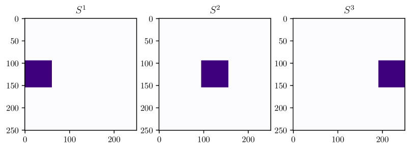
Figure 1: The three target resonator regions.

We specify three frequencies (i.e., $N=3$),

$$\omega=(30\pi,40\pi,50\pi),$$

at which to generate the specified modes by picking the propagation speed of the wave at each discretization point of the domain. We constrain the allowed propagation speed by picking

$$\theta^{\mathrm{min}}_{j}=1,\quad\theta^{\mathrm{max}}_{j}=2,\quad j=1,\dots,n.$$

Our discretization uses a $251\times 251$ grid, so $n=251^{2}=63001$, with $h=1/n$.

5.3 Physical design

We use ADMM to approximately solve the physical design problem, as in [LV13], using penalty parameter $\rho=100$. We initialized the method using the feasible structure and fields from §5.4, though similar designs are achieved with simple initializations like $\theta=\theta^{\mathrm{min}}$ and $z^{i}=0$, for $i=1,2,3$. We stop the algorithm when the physics constraint residual norm drops below a fixed tolerance of $10^{-2}$. The resulting locally optimized design is shown in figure 2 and the associated fields are shown in figure 3. In particular, after local optimization, we receive some $\theta$ and $z$ with

$$\theta^{\mathrm{min}}\leq\theta\leq\theta^{\mathrm{max}},~{}~{}\left\|(A+\mathop{\bf diag}(\theta))z-b\right\|_{2}\leq 10^{-2},$$

and then evaluate

$$p=\frac{1}{2}\sum_{i=1}^{3}\left\|{W^{i}(z^{i}-\hat{z}^{i})}\right\|_{2}^{2},$$

which gives $p=5145$.

Our non-optimized implementation required around 1.5 seconds per iteration and took 332 iterations to converge to the specified tolerance, so the total physical design time is a bit under 9 minutes on a 2015 2.9GHz dual core MacBook Pro. Our implementation used a sparse-direct solver; an iterative CG solver with warm-start would have been much faster.

5.4 Dual problem

We solved problem (9) using the Gurobi [GO18] SOCP solver and the JuMP [DHL17] mathematical modeling language for Julia [BEKS17]. Gurobi required under ten minutes to solve the dual problem, about the same time required by the physical design. This time, too, could be very much shortened; for example, we do not need to solve the dual problem to the high accuracy that Gurobi delivers.

The optimal dual value found is $d^{\star}=4733$, with the initial design and fields suggested by the optimal dual solution shown in figure 2 and figure 3, respectively.

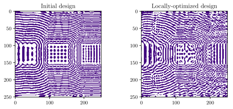
Figure 2: Left. Initial design suggested by the dual solution. Right. Optimized physical design.

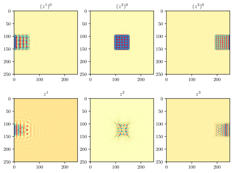
Figure 3: Top row. Fields suggested by solution to the dual problem. Bottom row. Fields in ADMM physical design. Columns show the three frequencies.

This tells us that

$$4733=d^{\star}\leq p^{\star}\leq p=5145,$$

which implies that our physical design objective value is no more than $(5145-4733)/4733\approx 8.7\%$ suboptimal. (We strongly suspect that $p^{\star}$ is closer to our design’s value, 5145, than the lower bound, 4733.)

6 Further extensions

There are several straightforward extensions of the above problem, which may yield useful results in specific circumstances. All of these problems have analytic forms for their Lagrange dual functions, and all forms generalize easily to their multi-frequency counterparts. Additionally, we explicitly derive the dual functions for some extensions which require a little more care.

Equality-constrained parameters.

Sometimes, it might be the case that a single design parameter might control several points in the domain of $z$—for example, in the case of Maxwell’s equations in two and three dimensions (see the appendix for more details), or when the domain’s grid size is much smaller than the smallest features that can be constructed.

Let $S_{k}\subseteq\{1,\dots,n\}$ for $k=1,\dots,m$ be a partition of indices, $\{1,\dots,n\}$. In other words, we want $S_{k}$ for $k=1,\dots,m$ to satisfy,

$$\bigcup_{k=1}^{m}S_{k}=\{1,\dots,n\}$$

and $S_{k}\cap S_{l}=\emptyset$ whenever $k\neq l$. These sets $S_{k}$ will indicate the sets of indices which are constrained to be equal—conversely, indices that are not constrained to be equal to any other indices are represented by singleton sets.

We can then write the new optimization problem as

$$\begin{array}[]{ll}\mbox{minimize}&\frac{1}{2}\left\|{W(z-\hat{z})}\right\|_{2}^{2}\\ \mbox{subject to}&(A+\mathop{\bf diag}(\theta))z=b\\ &\theta_{i}=\theta_{j},~{}\text{for all}~{}~{}i,j\in S_{k},~{}~{}k=1,\dots,m\\ &0\leq\theta\leq\theta^{\mathrm{max}}.\end{array}$$ (13)

To compute the Lagrange dual, let $I^{\prime}$ be an indicator function with $I^{\prime}(\theta)=0$ whenever $0\leq\theta\leq\theta^{\mathrm{max}}$ and $\theta_{i}=\theta_{j}$ for all $i,j\in S_{k}$ for $k=1,\dots,m$. Otherwise, $I^{\prime}(\theta)=+\infty$. We can write the new problem as problem (2) with the same Lagrangian as the one given in (3), replacing $I$ with $I^{\prime}$ in both expressions.

Minimization over $z$ is identical to (4) and minimization over $\theta$ is similar minus the fact that for each $k$, the indices found in $S_{k}$ are all constrained to be equal. Since the sum of convex quadratics is still a convex quadratic and, as before, since convex quadratics achieve minima at the boundary of an interval, we have

$$g(\nu)=-\frac{1}{2}\sum_{k=1}^{m}\max\Bigg{\{}\sum_{j\in S_{k}}W_{jj}^{-2}\left(a^{T}_{j}\nu-W^{2}_{jj}\hat{z}_{j}\right)^{2},\sum_{j\in S_{k}}W_{jj}^{-2}\big{(}a^{T}_{j}\nu+\nu_{j}\theta^{\mathrm{max}}_{j}- W^{2}_{jj}\hat{z}_{j}\big{)}^{2}\Bigg{\}}$$

$$-\nu^{T}b+\frac{1}{2}\left\|{W\hat{z}}\right\|_{2}^{2},$$

as the final Lagrange dual function. The corresponding dual problem can be written as a convex QCQP.

Field constraints.

In the case where (1) has field constraints, i.e.,

$$\begin{array}[]{ll}\mbox{minimize}&\frac{1}{2}\left\|{W(z-\hat{z})}\right\|_{2}^{2}\\ \mbox{subject to}&(A+\mathop{\bf diag}(\theta))z=b\\ &(z_{j}-h_{j})^{2}\leq(z^{\mathrm{max}}_{j})^{2},~{}~{}j=1,\dots,n\\ &0\leq\theta\leq\theta^{\mathrm{max}},\end{array}$$

for some $h\in{\mbox{\bf R}}^{n}$, the construction also parallels the one given in §3. The resulting dual optimization problem, in comparison to problem (7), cannot be written as a QCQP—it is, instead, a more general SOCP.

Regularizers.

It is also possible to add a separable regularization term for $\theta$, the parametrization of the device; for example, in the case where we would want to bias specific $\theta_{j}$ towards either $0$ or $\theta^{\mathrm{max}}_{j}$.

If we have a family of concave functions, $r_{j}:{\mbox{\bf R}}\to{\mbox{\bf R}}$ such that our regularizer can be written as a function of the form

$$\theta\mapsto\sum_{j=1}^{n}r_{j}(\theta_{j}),$$

(one such example is a linear function of $\theta$), then the problem becomes

$$\begin{array}[]{ll}\mbox{minimize}&\frac{1}{2}\left\|{W(z-\hat{z})}\right\|_{2}^{2}+\sum_{j=1}^{n}r_{j}(\theta_{j})\\ \mbox{subject to}&(A+\mathop{\bf diag}(\theta))z=b\\ &0\leq\theta\leq\theta^{\mathrm{max}}.\end{array}$$

By using the fact that $r_{j}$ is concave and therefore achieves a minimum over an interval at the boundary of the interval, it is possible to derive a bound that parallels (6).

Parameter perturbations.

In some cases (e.g., when considering temperature perturbations), it might be very natural to have a physical constraint of the form

$$(A+D\mathop{\bf diag}(\theta))z=b,$$

where $D\in{\mbox{\bf R}}^{n\times n}$ is a diagonal matrix that is not necessarily invertible. In other words, our new problem is

$$\begin{array}[]{ll}\mbox{minimize}&\frac{1}{2}\left\|{W(z-\hat{z})}\right\|_{2}^{2}\\ \mbox{subject to}&(A+D\mathop{\bf diag}(\theta))z=b\\ &0\leq\theta\leq\theta^{\mathrm{max}}.\end{array}$$

Directly applying the method from §3 yields a similar explicit form for $g$ as given in (6).

Indeterminate eigenvalue.

In the case where we want $z$ to be a mode of the device with some unspecified eigenvalue $\lambda$ with upper and lower limits $\lambda^{\mathrm{min}}\leq\lambda\leq\lambda^{\mathrm{max}}$, we can write the problem as

$$\begin{array}[]{ll}\mbox{minimize}&\frac{1}{2}\left\|{W(z-\hat{z})}\right\|_{2}^{2}\\ \mbox{subject to}&(A+\lambda I+\mathop{\bf diag}(\theta))z=b\\ &\lambda^{\mathrm{min}}\leq\lambda\leq\lambda^{\mathrm{max}}\\ &0\leq\theta\leq\theta^{\mathrm{max}}.\end{array}$$ (14)

To construct the dual, note that the Lagrangian of this problem is similar to the Lagrangian of problem (1),

$$\mathcal{L}(z,\theta,\lambda,\nu)=\frac{1}{2}\left\|{W(z-\hat{z})}\right\|_{2}^{2}+I(\theta)+\nu^{T}((A+\lambda I+\mathop{\bf diag}(\theta))z-b).$$

We will define the partial Lagrangian, $\mathcal{L}^{p}$ to be the infimum of $\mathcal{L}$ with respect to $z$ and $\theta$, leaving $\lambda$ and $\nu$ as free variables. The solution to the partial minimization of $\mathcal{L}$ is given in (6),

$$\mathcal{L}^{p}(\lambda,\nu) =\inf_{z,\theta}\mathcal{L}(z,\theta,\lambda,\nu)$$

$$=-\frac{1}{2}\sum_{j=1}^{n}W_{jj}^{-2}\max_{\theta_{j}\in\{0,\theta^{\mathrm{max}}_{j}\}}\left(a^{T}_{j}\nu+(\lambda+\theta_{j})\nu_{j}-W^{2}_{jj}\hat{z}_{j}\right)^{2}-\nu^{T}b+\frac{1}{2}\left\|{W\hat{z}}\right\|_{2}^{2}.$$

As $\mathcal{L}^{p}(\lambda,\nu)$ is a concave in $\lambda$, it achieves its minimum at the boundaries of the domain of $\lambda$. So, since

$$g(\nu)=\inf_{\lambda^{\mathrm{min}}\leq\lambda\leq\lambda^{\mathrm{max}}}\mathcal{L}^{p}(\lambda,\nu),$$

we can write,

$$g(\nu)=\min_{\lambda\in\{\lambda^{\mathrm{min}},\,\lambda^{\mathrm{max}}\}}\mathcal{L}^{p}(\lambda,\nu)$$

which is the minimum over a (finite) number of concave functions. The corresponding dual problem can then be expressed as a convex QCQP.

7 Conclusion

This paper has derived a set of lower bounds for a general class of physical design problems, making it possible to give (a) an easily-computable certificate that certain objectives cannot be physically achieved and (b) a bound on how suboptimal (relative to the global optimum) a given design could be. Additionally, as a side-effect of computing this lower bound, we also receive an initialization for any heuristic approach we might take for approximately solving (1) or its multi-frequency version (8).

Additionally, it seems feasible to obtain asymptotic bounds with respect to physical parameters (e.g., with respect to the size of the device) via this approach, since the optimization problem in (7) can easily be written in an unconstrained form. In other words, picking any $\nu\in{\mbox{\bf R}}^{n}$ will yield some lower bound, and an appropriate choice might yield scaling laws that could be useful as general rules-of-thumb in inverse design.

8 Appendix

8.1 Optimization using ADMM

We can approximately minimize (1) via the alternating direction method of multipliers, as in [LV13]. The method proceeds by forming the augmented Lagrangian of (1) and minimizing over each available variable, before updating a dual variable after each iteration.

ADMM iteration.

We form the augmented lagrangian of problem (1) as in [BPC⁺11b].

$$\mathcal{L}^{\mathrm{aug}}(z,\theta;\nu)=\frac{1}{2}\left\|{W(z-\hat{z})}\right\|_{2}^{2}+\frac{\rho}{2}\left\|{(A+\mathop{\bf diag}(\theta))z-b+\nu}\right\|_{2}^{2},$$

where $\rho>0$ is a penalty parameter we set. Minimizing over each of $z$ and $\theta$ (with the constraint $0\leq\theta\leq\theta^{\mathrm{max}}$) yields the following update rules

$$z^{(k+1)} =(W^{2}+\rho A(\theta^{(k)})^{T}A(\theta^{(k)}))^{-1}(W^{2}\hat{z}+\rho A(\theta^{(k)})^{T}(b-\nu^{(k)}))$$

$$\theta^{(k+1)}_{i} =S((b_{i}-a_{i}^{T}z^{(k+1)}-\nu_{i}^{(k)})/z^{(k+1)}_{i},\theta^{\mathrm{max}}_{i}),~{}~{}i=1,\dots,n$$

$$\nu^{(k+1)} =\nu^{(k)}+A(\theta^{(k+1)})z^{(k+1)}-b,$$

where we have defined $A(\theta)=A+\mathop{\bf diag}(\theta)$ and $S(x,u)=\min\{\max\{x,0\},u\}$ is the clamp function with upper limit, $u$, and we arbitrarily define $S(x/0,u)=0$ for any $x$, though any value in $[0,u]$ would similarly suffice.

It can be shown that, if a feasible field exists for some $\theta$, then, as $k\to\infty$, the iterates converge to a locally-optimal design $\theta$ and feasible field $z$, for an appropriately large choice of penalty parameter $\rho$ [GGC18]. In practice, we find that ADMM is fairly robust and converges for a large range of values of $\rho$, though some choices appear to increase convergence speed.

8.2 Formulations of physical problems

Here, we describe ways of mapping the photonic inverse design problem into extensions of problem (1).

Maxwell’s equations in three dimensions.

Ampere’s law and Faraday’s law in Maxwell’s equations, for a specific frequency $\omega$, can be written as

$$\nabla\times H =-\mathbf{i}\omega\varepsilon E+J$$ (15)

$$\nabla\times E =\mathbf{i}\omega\mu H,$$ (16)

over some compact region of space $\Omega\subset{\mbox{\bf R}}^{3}$, with appropriate boundary conditions for $H$ and $E$. Here, $E,H,J:\Omega\to\mathbf{C}^{3}$ are the electric field, magnetic field, and the current density, respectively, $\varepsilon,\mu:\Omega\to{\mbox{\bf R}}_{+}$ are the permittivity and permeability of the space (which we can often control by an appropriate choice of material), respectively. The bold $\mathbf{i}$—to avoid confusion with the index $i$—is the imaginary unit with $\mathbf{i}^{2}=-1$. We will also assume that we can choose any permittivity and permeability that satisfy $\varepsilon^{\mathrm{min}}(x)\leq\varepsilon(x)\leq\varepsilon^{\mathrm{max}}(x)$ and $\mu^{\mathrm{min}}(x)\leq\mu(x)\leq\mu^{\mathrm{max}}(x)$ at each point of the region $x\in\Omega$.

8.2.1 Constant permeability

In many physical design problems, $\mu$ is also a constant that is independent of our material choice (e.g., in the case where we are choosing between silicon or air, under small magnetic field) and constant through space (i.e., $\mu(x)=\mu_{c}$ for $x\in\Omega$). Assuming this is true, we can write

$$\nabla\times\nabla\times E=\mathbf{i}\omega\mu_{c}\nabla\times H=\omega^{2}\mu\varepsilon E+\mathbf{i}\omega\mu_{c}J,$$

by taking the curl of (16) and plugging in (15). Rearranging gives,

$$-\nabla\times\nabla\times E+\omega^{2}\mu_{c}\varepsilon E=-\mathbf{i}\omega\mu_{c}J.$$ (17)

All we require is a discretization of $E$, $\varepsilon$, $J$, and the linear operator $-(\nabla\times\nabla\times\cdot)$. There are several standard ways of doing this (e.g., the Yee lattice, see [Che95, §4.6.4]), though any method which discretizes the linear operator in the space will suffice. Let $z\in\mathbf{C}^{3n}$ be the optimization variable corresponding to the discretized field with $z^{i}\in\mathbf{C}^{n}$ being the field along each of the three axes, $i=1,2,3$. Then, we can rewrite and discretize (17) as

$$\big{(}\underbrace{-\nabla\times\nabla\times}_{A}+\omega^{2}\mu_{c}\varepsilon\big{)}\underbrace{E}_{z}=\underbrace{-\mathbf{i}\omega\mu_{c}J}_{b}.$$

Here, each of $A\in\mathbf{C}^{3n\times 3n}$ and $b\in\mathbf{C}^{3n}$ are the corresponding discretizations of the variables they are below.

The next question is: how can we deal with the scalar permittivity term? One simple way is to allow $\theta\in\mathbf{C}^{3n}$—which roughly corresponds to the discretized version of $\omega^{2}\mu_{c}\varepsilon$—to have a component along each axis, which we will call $\theta^{i}$ for $i=1,2,3$, and to then constrain all axes to be equal—i.e., $\theta^{1}=\theta^{2}=\theta^{3}$. Using this idea, we can then write $\mathop{\bf diag}(\theta)z$, as a discretization of $\omega^{2}\mu_{c}\varepsilon E$. Note that, without the equality constraint, $\theta$ would be allowed to vary arbitrarily along each axis.

Finally, we set $\theta^{\mathrm{max}}$ to be the largest possible value of $\omega^{2}\mu_{c}\varepsilon$ at each point in the discretization (with a similar case for $\theta^{\mathrm{min}}$), which lets us write the final program as a special case of (13),

$$\begin{array}[]{ll}\mbox{minimize}&\frac{1}{2}\left\|{W(z-\hat{z})}\right\|_{2}^{2}\\ \mbox{subject to}&(A+\mathop{\bf diag}(\theta))z=b\\ &\theta^{1}=\theta^{2}=\theta^{3},\\ &\theta^{\mathrm{min}}\leq\theta^{i}\leq\theta^{\mathrm{max}},~{}~{}i=1,2,3.\end{array}$$

8.2.2 Arbitrary permeability

In the case where we are also allowed to vary the permeability throughout the space, we can discretize the equations in a similar way. The resulting system will have roughly double the size, but is still—usually, depending on the choice of discretization—relatively sparse.

First, we can write equations (15) and (16) in the suggestive form

$$\begin{bmatrix}\nabla\times&0\\ 0&\nabla\times\end{bmatrix}\begin{bmatrix}E\\ H\end{bmatrix}+\mathbf{i}\omega\begin{bmatrix}\varepsilon I&0\\ 0&-\mu I\end{bmatrix}\begin{bmatrix}E\\ H\end{bmatrix}=\begin{bmatrix}J\\ 0\end{bmatrix},$$ (18)

where $I\in{\mbox{\bf R}}^{3\times 3}$ is the identity matrix. From here, we can perform a similar trick as in §8.2.1, by rewriting and discretizing (18) in the following way:

$$\Bigg{(}-\mathbf{i}\omega^{-1}\underbrace{\begin{bmatrix}\nabla\times&0\\ 0&\nabla\times\end{bmatrix}}_{A}+\begin{bmatrix}\varepsilon I&0\\ 0&-\mu I\end{bmatrix}\Bigg{)}\underbrace{\begin{bmatrix}E\\ H\end{bmatrix}}_{z}=\underbrace{-\mathbf{i}\omega^{-1}\begin{bmatrix}J\\ 0\end{bmatrix}}_{b},$$

where $A\in\mathbf{C}^{6n\times 6n}$, $z\in\mathbf{C}^{6n}$, and $b\in\mathbf{C}^{6n}$ are the discretized versions of the expressions above each. We will write $z_{E}^{i}$ for $i=1,2,3$ to be the $i$th component of the discretization of the $E$-field, with a similar definition for $z_{H}^{i}$.

As before, let $\theta_{E}^{i}\in{\mbox{\bf R}}^{n}$ and $\theta_{H}^{i}\in{\mbox{\bf R}}^{n}$ be the discretization of the permittivity and permeability, respectively, along each axis $i=1,2,3$, with $\theta$ being the concatenation of each component and field over all points in the discretization. To ensure that the permittivity and permeability all remain scalar quantities, we simply constrain each entry of $\theta$ to be equal along all axes at each discretization point, which yields a problem which is a special case of (13):

$$\begin{array}[]{ll}\mbox{minimize}&\frac{1}{2}\left\|{W(z-\hat{z})}\right\|_{2}^{2}\\ \mbox{subject to}&(A+\mathop{\bf diag}(\theta))z=b\\ &\theta^{1}_{E}=\theta^{2}_{E}=\theta^{3}_{E},\\ &\theta^{1}_{H}=\theta^{2}_{H}=\theta^{3}_{H},\\ &\theta^{\mathrm{min}}_{E}\leq\theta^{i}_{E}\leq\theta^{\mathrm{max}}_{E},~{}~{}i=1,2,3,\\ &\theta^{\mathrm{min}}_{H}\leq\theta^{i}_{H}\leq\theta^{\mathrm{max}}_{H},~{}~{}i=1,2,3,\end{array}$$

where $\theta^{\mathrm{min}}_{E}$ is defined to be the minimum value of $\varepsilon$ at each discretization point with a similar definition for $\theta^{\mathrm{max}}_{E}$, $\theta^{\mathrm{max}}_{H}$, $\theta^{\mathrm{min}}_{H}$.

References

- [AVDB18] Akshay Agrawal, Robin Verschueren, Steven Diamond, and Stephen Boyd. A rewriting system for convex optimization problems. Journal of Control and Decision, 5(1):42–60, 2018.
- [BEKS17] Jeff Bezanson, Alan Edelman, Stefan Karpinski, and Viral B. Shah. Julia: A fresh approach to numerical computing. SIAM review, 59(1):65–98, 2017.
- [BPC+11a] Stephen Boyd, Neal Parikh, Eric Chu, Borja Peleato, Jonathan Eckstein, et al. Distributed optimization and statistical learning via the alternating direction method of multipliers. Foundations and Trends in Machine learning, 3(1):1–122, 2011.
- [BPC+11b] Stephen Boyd, Neal Parikh, Eric Chu, Borja Peleato, Jonathan Eckstein, et al. Distributed optimization and statistical learning via the alternating direction method of multipliers. Foundations and Trends® in Machine learning, 3(1):1–122, 2011.
- [BV04] Stephen Boyd and Lieven Vandenberghe. Convex optimization. Cambridge university press, 2004.
- [BW13] Max Born and Emil Wolf. Principles of optics: electromagnetic theory of propagation, interference and diffraction of light. Elsevier, 2013.
- [Che95] Weng C. Chew. Waves and fields in inhomogeneous media. IEEE press, 1995.
- [DCB13] Alexander Domahidi, Eric Chu, and Stephen Boyd. ECOS: An SOCP solver for embedded systems. In Control Conference (ECC), 2013 European, pages 3071–3076. IEEE, 2013.
- [DHL17] Iain Dunning, Joey Huchette, and Miles Lubin. JuMP: A modeling language for mathematical optimization. SIAM Review, 59(2):295–320, 2017.
- [Fer36] Enrico Fermi. Thermodynamics. Snowball Publishing, 1936.
- [GGC18] Wenbo Gao, Donald Goldfarb, and Frank E. Curtis. ADMM for multiaffine constrained optimization. arXiv preprint arXiv:1802.09592, 2018.
- [GO18] LLC Gurobi Optimization. Gurobi optimizer reference manual, 2018.
- [HG12] Raphael T. Haftka and Zafer Gürdal. Elements of structural optimization, volume 11. Springer Science & Business Media, 2012.
- [LKBMY13] Christopher M. Lalau-Keraly, Samarth Bhargava, Owen D. Miller, and Eli Yablonovitch. Adjoint shape optimization applied to electromagnetic design. Optics express, 21(18):21693–21701, 2013.
- [LV10] Jesse Lu and Jelena Vučković. Inverse design of nanophotonic structures using complementary convex optimization. Optics express, 18(4):3793–3804, 2010.
- [LV13] Jesse Lu and Jelena Vučković. Nanophotonic computational design. Optics express, 21(11):13351–13367, 2013.
- [LVBL98] Miguel S. Lobo, Lieven Vandenberghe, Stephen Boyd, and Hervé Lebret. Applications of second-order cone programming. Linear algebra and its applications, 284(1-3):193–228, 1998.
- [MLP+18] Sean Molesky, Zin Lin, Alexander Y. Piggott, Weiliang Jin, Jelena Vučković, and Alejandro W. Rodriguez. Inverse design in nanophotonics. Nature Photonics, 12(11):659, 2018.
- [MPR+16] Owen D. Miller, Athanasios G. Polimeridis, M.T. Homer Reid, Chia Wei Hsu, Brendan G. DeLacy, John D. Joannopoulos, Marin Soljačić, and Steven G. Johnson. Fundamental limits to optical response in absorptive systems. Optics express, 24(4):3329–3364, 2016.
- [NUS+10] Daniel Noreland, Rajitha Udawalpola, Pablo Seoane, Eddie Wadbro, and Martin Berggren. An efficient loudspeaker horn designed by numerical optimization: an experimental study. Report UMINF, 10, 2010.
- [OCPB16a] Brendan O’Donoghue, Eric Chu, Neal Parikh, and Stephen Boyd. Conic optimization via operator splitting and homogeneous self-dual embedding. Journal of Optimization Theory and Applications, 169(3):1042–1068, 2016.
- [OCPB16b] Brendan O’Donoghue, Eric Chu, Neal Parikh, and Stephen Boyd. SCS: Splitting conic solver, version 1.2. 6, 2016.
- [Pur77] Edward M. Purcell. Life at low Reynolds number. American journal of physics, 45(1):3–11, 1977.
- [SFJM18] Hyungki Shim, Lingling Fan, Steven G. Johnson, and Owen D. Miller. Fundamental limits to near-field optical response, over any bandwidth. arXiv preprint arXiv:1805.02140, 2018.