Equation of state in (2+1) flavor QCD at high temperatures

Abstract:

We calculate the Equation of State at high temperatures in (2+1) flavor QCD using the highly improved staggered quark (HISQ) action. We study the lattice spacing dependence of the pressure at high temperatures using lattices with temporal extent $N_{\tau}=6,~{}8,~{}10$ and $12$ and perform continuum extrapolations. We also give a continuum estimate for the Equation of State up to temperatures $T=2$ GeV, which are then compared with results of the weak-coupling calculations. We find reasonable agreement with the HTL calculation at the highest temperatures and a tension with the EQCD calculation of a few percent, with the lattice results in the middle between both.

1 Introduction

Ab initio calculations of the QCD Equation of State (EoS) at vanishing baryon density have been in the focus of research for more than a decade, see [1, 2, 3, 4, 5, 6, 7] and references therein. These calculations were performed with different varieties of improved staggered fermions, nearly physical quark masses and 2+1 or 2+1+1 flavors of sea quarks. As a result, the EoS in the continuum limit has been determined for 2+1 flavors using two different staggered discretizations (HISQ [8] and stout) up to temperatures of about $T=400\,{\rm MeV}$ [4, 5] and for 2+1+1 flavors using only the stout formulation up to temperatures of about $T=1\,{\rm GeV}$ [6].

Overall the different 2+1 flavor calculations are in good agreement, although there is a slight tension at the highest temperatures. By comparing the 2+1 and 2+1+1 flavor calculations using the stout formulation it was concluded that the contribution from the charm sea is already significant at $T\approx 400\,{\rm MeV}$. However, as the presence of the charm quark in the sea may lead to a suppression of the other contributions to the EoS, the overall effect may be subject to subtle compensations. Moreover, the 2+1 and 2+1+1 flavor results are compared in the region where the tension between both formulations has been found. From this discussion it is clear that dynamical charm quarks should be included in the lattice determination of the EoS at higher temperatures for use in phenomenology and that an independent calculation is desirable. Efforts in this direction with the HISQ formulation are still on-going [9]. In particular, the large discretization errors associated with the charm quark mass strongly suggest that such a calculation should be performed with the HISQ action. Yet the 2+1 flavor EoS is needed with higher precision for a robust, quantitative determination of the correct charm contribution to the pressure including all of the subtle effects.

For a comparison to weak-coupling calculations a lattice determination without the charm quark may actually be advantageous. This is evident from the absence of massive quark degrees of freedom in the weak-coupling calculations [10, 11] at the highest available order, NNNLO. At temperatures in the range between $T\approx 400\,{\rm MeV}$ and some multiple of the charm quark mass, $m_{c}\equiv m_{c}(m_{c})=1.277(10)\,{\rm GeV}$ [12], corrections due to the finite charm quark mass are almost certainly relevant and large. Unless the applicability of weak coupling is firmly established for the respective observables at these temperatures, there is a risk of conflating the uncertainties associated with the temperature scale with those of the charm mass corrections. Precise results with 2+1 flavors at high temperatures from the lattice alleviate the concerns regarding applicability of weak coupling considerably and establish a robust baseline for determining the actual charm quark contribution.

For these reasons we extend the previous calculations of the 2+1 flavor EoS using the HISQ formulation to higher temperatures. We use lattices with larger light sea quark mass, $m_{l}=m_{s}/5$ (compared to $m_{l}=m_{s}/20$ in [5]), and discuss the light quark mass dependence of the trace anomaly. We discuss the cutoff dependence of the trace anomaly and the pressure in detail and determine the continuum limit or continuum estimates using different strategies. The rest of this paper is organized as follows. In Sec. 2, we discuss the details of the lattice calculations. In Sec. 3, we discuss the trace anomaly and its cutoff effects. In Sec. 4, we obtain results for the pressure and scrutinize its cutoff effects. We compare to weak-coupling results in Sec. 5 and conclude in Sec. 6.

2 Details of the lattice calculations

The objective of our research is extending the calculation of the 2+1 flavor QCD Equation of State in [5] to higher temperatures and compare the EoS to results obtained in the weak-coupling limit. Following [5] we use the tree-level improved Symanzik gauge action and the Highly Improved Staggered Quark (HISQ) action for quarks. We use gauge ensembles at finite temperature with $N_{\tau}=12,\ 10,\ 8,\ 6$ and $4$, which have been generated for studies of the pseudocritical temperature [13] and the EoS [5] by the HotQCD collaboration, and for studies of the entropy shift due to a heavy quark in the thermal medium [14] and color screening [15] by the TUMQCD collaboration.

In order to cancel the UV divergences in the trace anomaly at $T>0$, we subtract the trace anomaly at $T=0$ using the same bare parameters. We use gauge ensembles at $T=0$ from the HotQCD collaboration [5, 13] with a pion mass of $m_{\pi}=160\,{\rm MeV}$ in the continuum limit. Since the corresponding lattice spacings are insufficient for reaching higher temperatures with small discretization errors, i.e. large $N_{\tau}$, we generated new ensembles with finer lattice spacing but larger pion mass, $m_{\pi}=320\,{\rm MeV}$ [7]. We use the rational hybrid Monte Carlo at five values of the coupling, $\beta=10/g^{2}$, see Tab. 1 for the parameters.

$\beta$	$m_{s}$	vol	a [fm]	# traj.
7.030	0.03560	$48^{4}$	0.08253	1890
7.825	0.01542	$64^{4}$	0.04036	1265
8.000	0.01299	$64^{4}$	0.03469	3927
8.200	0.01071	$64^{4}$	0.02924	3927
8.400	0.00887	$64^{4}$	0.02467	3927

Table 1: The parameters of the zero temperature gauge ensembles.

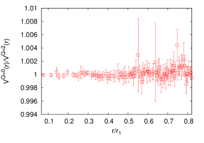
For the three finest ensembles, $\beta\geq 8$, topological tunneling only takes place during pre-thermalized molecular dynamics evolution, but is too suppressed after thermalization. We have generated multiple streams of MD trajectories with the same lattice parameters that randomly stall in different topological sectors, $Q\in\{0,1,2\}$. We find among the observables contributing to the EoS only for the light quark condensate $\braket{\bar{\psi}\psi}_{l}$ a statistically significant dependence on the topological charge $Q$. The respective changes of the light quark contribution to the trace anomaly are smaller than the statistical error of the much larger contribution from the gauge action. We show in the left panel of Fig. 1 that the static energy is consistent for different values of $Q$ in the finest ensemble $\beta=8.4$. For the other ensembles the picture is similar. We conclude that systematic errors due to frozen topology are numerically irrelevant for our study.

Figure 1: The static energy for different topological charges $Q=0$ or $2$ with $\beta=8.4$ (left) or light quark masses $m_{s}/5$ or $m_{s}/20$ with $\beta=7.825$ (right) is consistent at 0.1% level for $r\leq 0.8r_{1}$. We see a consistent trend towards larger values of the static energy for the larger mass, but no trend for variation of $Q$.

We fix the lattice scale with the static energy, i.e. we calculate $r_{1}$ and $r_{2}$ defined via

$$r^{2}\left.\frac{dV(r)}{dr}\right|_{r=r_{1}}=1, r^{2}\left.\frac{dV}{dr}\right|_{r=r_{2}}=\frac{1}{2},$$ (1)

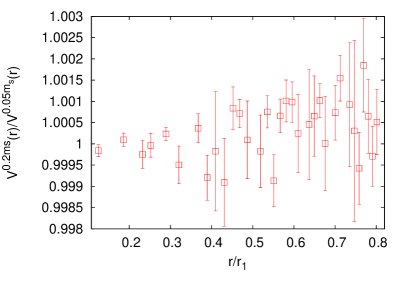
where $r_{1}=0.3106\,{\rm fm}$ and $r_{2}=0.1413\,{\rm fm}$. For the two ensembles corresponding to coarser lattices we can directly compare to previous calculations by HotQCD with a smaller pion mass. This permits us to determine quark mass effects in the lattice scale as well as in the thermodynamic observables. The static energy changes slightly for the larger quark mass, see Fig. 1, and thus, the lattice scale $r_{1}$ is 0.7% or 1.6% lower $\beta=7.03$ or $7.825$, respectively. Since the scale $r_{2}$ is only 0.3% lower for $\beta=7.825$ we use $r_{2}$ to set the scale for the finer ensembles, which is consistent with the non-perturbative beta function of [5]. The observed variation of the static energy due to the frozen topology charge is smaller than the quark mass dependence and safely covered within the statistical errors. Cominbing the new and old results for the lattice scale we obtain a consistent beta function with smaller uncertainty [7], which we parameterize with an Allton-type Ansatz

$$\frac{r_{1}}{a}=\frac{c_{0}f(\beta)+c_{2}(10/\beta)f^{3}(\beta)}{1+d_{2}(10/\beta)f^{2}(\beta)}, f((\beta)=\left(\frac{10b_{0}}{\beta}\right)^{-\frac{b_{1}}{2b_{0}^{2}}}e^{-\frac{\beta}{20b_{0}}},$$ (2)

where $b_{0}=9/(16\pi^{2})$ and $b_{1}=1/(4\pi^{4})$. The other coefficients $c_{0}=43.12(18)$, $c_{2}=347008(32131)$ and $d_{2}=5584(599)$ are determined with a fit, see [7]. In our analysis we combine ensembles with different quark masses, using the ensembles with larger pion mass for the UV subtraction only at high temperatures, $T\gtrsim 470\,{\rm MeV}$, where numerical effects of $m_{l}$ are known to be small for $m_{l}<0.4m_{s}$ [3]. Due to $T=1/(aN_{\tau})$ these ensembles provide access up to $T=2\,{\rm GeV}$ with $N_{\tau}=4$.

3 Trace anomaly

In order to obtain the 2+1 flavor QCD Equation of State we first calculate the trace anomaly, i.e. the trace of the energy-momentum tensor, $\Theta^{\mu\mu}=\epsilon-3p$ on the lattice. $\Theta^{\mu\mu}$ can be expressed in terms of the expectation values of the gauge action and the scalar condensates of the quark flavors in the sea, i.e. light and strange. Since these densities diverge linearly in the continuum limit, we consider differences between the results at zero temperature and at finite temperature. Finally, we account for multiplicative renormalization bu rescaling these differences with the non-perturbative beta function $R_{\beta}$ and mass renormalization function $R_{m}$. For the HISQ action we may write

$$\Theta^{\mu\mu}(T) =\Theta^{\mu\mu}_{G}(T)+\Theta^{\mu\mu}_{F}(T),$$ (3)

$$\frac{\Theta^{\mu\mu}_{G}(T)}{T^{4}}, =R_{\beta}\left\{\braket{S_{G}}_{T=0}-\braket{S_{G}}_{T>0}\right\}N_{\tau}^{4},$$ (4)

$$\frac{\Theta^{\mu\mu}_{F}(T)}{T^{4}} =-R_{\beta}R_{m}\left\{2m_{l}\left(\braket{\bar{\psi}\psi}_{l,T=0}-\braket{\bar{\psi}\psi}_{l,T>0}\right)+m_{s}\left(\braket{\bar{\psi}\psi}_{s,T=0}-\braket{\bar{\psi}\psi}_{s,T>0}\right)\right\}N_{\tau}^{4}$$ (5)

using the same notation as in [5]. $R_{\beta}$ and $R_{m}$ are defined via

$$R_{\beta}(\beta)=\frac{r_{1}}{a}\left(\frac{d(r_{1}/a)}{d\beta}\right)^{-1}, R_{m}(\beta)=\frac{1}{m_{s}(\beta)}\left(\frac{dm_{s}(\beta)}{d\beta}\right),$$ (6)

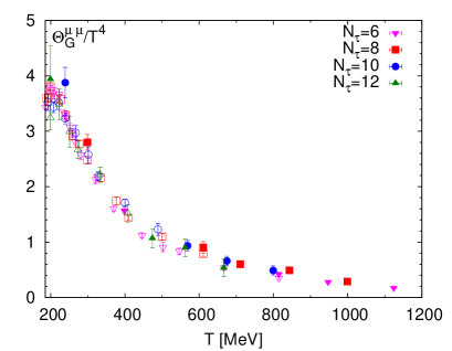
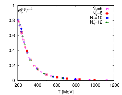
$\Theta^{\mu\mu}_{G}$ is much larger than $\Theta^{\mu\mu}_{F}$. We show the two contributions to the trace anaomaly in Fig. 2. The gauge field contribution, which we show in the left panel, is systematically larger for the ensembles with larger sea quark mass. Although we cannot correct for this implicit quark mass dependence, the difference is covered by the statistical errors for temperatures above $T\gtrsim 400\,{\rm MeV}$, i.e. in the range where we use these data. For $N_{\tau}\geq 8$ discretization errors are quite visible, but mostly covered by the rather large statistical errors in this temperature window. The fermion contribution, which we show in the right panel, has an explicit dependence on the sea quark mass. As we use a value $m_{l}=m_{s}/20$ instead of $m_{l}=m_{s}/5$ in (5) to account for this, we cannot resolve a residual quark mass dependence in $\Theta^{\mu\mu}_{F}$ anymore for $T\gtrsim 400\,{\rm MeV}$. Moreover, statistical errors and cutoff effects are very small.

Figure 2: The gauge part (left) and the fermion part (right) of the trace anomaly obtained with HISQ action. The open symbols correspond to HotQCD results with $m_{l}/m_{s}=1/20$ [5], while the filled symbols correspond to $m_{l}/m_{s}=1/5$.

We separately discuss the trace anomaly for low and high temperatures.

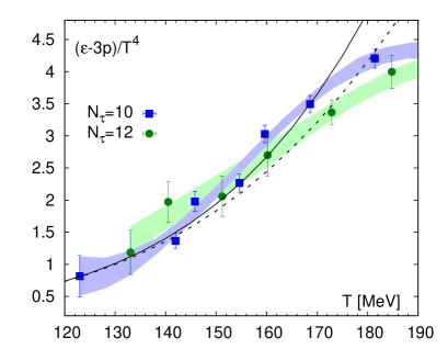
We revisit the low temperature results for the trace anomaly since we require higher precision at low temperatures in order to take the continuum limit in terms of the pressure. In this study we use gauge ensembles at low temperatures with high statistics that have been generated for a study of the Polyakov loop in the crossover region by the TUMQCD collaboration [14]. These ensembles provide access to $T=123\,{\rm MeV}$ with $N_{\tau}=10$ and to $T=133\,{\rm MeV}$ as well as $T=140\,{\rm MeV}$ with $N_{\tau}=12$. We show our low temperature results for the trace anomaly with $N_{\tau}=12$ and $10$ in the left panel of Fig. 3 together with bands obtained from interpolating splines whose errors have been estimated from the bootstrap method. The difference between both in the window $160\,{\rm MeV}<T<180\,{\rm MeV}$ is indicative of rather large cutoff effects. We compare our results directly to predictions of hadron resonance gas (HRG) models. Namely, we consider a model with only the states listed by the PDG – labeled HRG-PDG – and a model including also missing states, i.e. states predicted by the quark model that have not been confirmed experimentally – labeled HRG-QM. We find good agreement of both HRG models with the data up to $T<140\,{\rm MeV}$. For higher temperatures the difference between both models is significantly and they cannot describe the data well.

Figure 3: Left: The trace anomaly calculated in the low temperature region. The bands correspond to interpolations. The dashed line corresponds to HRG-PDG, while the solid line corresponds to HRG-QM. Right: The numerical results for the trace anomaly in the high temperature region at two different quark masses. The bursts correspond to calculations with p4 action and $m_{l}=m_{s}/10$ [1].

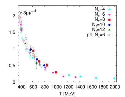
At high temperatures $T>400\,{\rm MeV}$, discretization errors and quark mass dependendence are very much suppressed. We show the HISQ results together with older results obtained with the p4 action and a quark mass of $m_{l}=m_{s}/10$. Whereas the results with $N_{\tau}=4$ and $N_{\tau}=6$ are systematically lower, the results for $N_{\tau}\geq 8$ do not depend on $N_{\tau}$ or the light quark mass within their uncertainties. The smallness of the cutoff effects can be understood from the weak-coupling picture, where the trace anomaly has discretization errors starting at three-loop order, i.e. $\mathcal{O}(\alpha_{\mathit{s}}^{2})$. Since the running of $\alpha_{\mathit{s}}$ is controlled by the temperature, discretization errors are strongly suppressed at high temperatures and their respective temperature dependence is mild, i.e. logarithmic.

4 Pressure

Eventually we obtain the Equation of State and the pressure from $\Theta^{\mu\mu}$ via the integral method,

$$\frac{p}{T^{4}}-\frac{p_{0}}{T_{0}^{4}}=\int\limits_{T_{0}}^{T}dT^{\prime}\frac{\Theta^{\mu\mu}}{T^{\prime\,5}}.$$ (7)

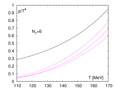
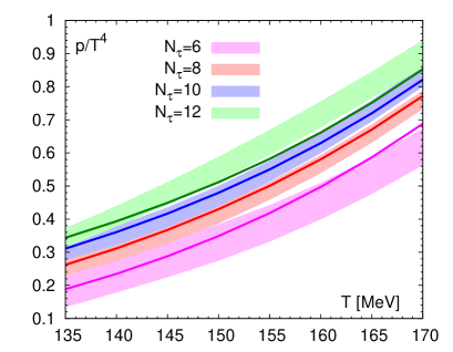
Here, we assume that we know the pressure $p(T_{0})$ at the reference temperature $T_{0}$. If $T_{0}$ is sufficiently small, the pressure may be set to zero or taken from a calculation using an HRG model. For the temperature range in our simulations, we have to adhere to the latter case. Moreover, we have to account in the HRG for the cutoff effects due to distortion of the hadron spectrum with the HISQ formulation. In short, for each species of hadrons there are multiple tastes of the same hadron with masses that are enlarged by discretization errors to varying degree. This distortion is most severe in the sector of pseudo-Goldstone bosons. Hadrons with larger masses contribute less to the pressure. The effect of this distortion is suppressed in the trace anomaly since hadrons with larger masses contribute more strongly to the trace anomaly and partly compensate for the distortion. We use the HRG-QM where only the pseudo-Goldstone bosons are modified, and estimate a systematic uncertainty from the difference to the HRG-QM where all ground states or all ground and excited states are modified, see [7] for a more detailed discussion. In the left panel of Fig. 4 we show the lattice result for the pressure at low temperatures together with a prediction of the HRG with a distorted spectrum. In the right panel, we show the lattice QCD results obtained via the integral method together with the HRG prediction.

Figure 4: Left: The pressure with $N_{\tau}=6$ for HRG with different distortions of the hadron spectrum. Right: The lines correspond to HRG with distorted hadron spectrum (see text).

We summarize the reference temperatures and pressures for different $N_{\tau}$ in Tab. 2.

$N_{\tau}$	$T_{0}$ [MeV]	$p(T_{0},N_{\tau})$
6	135	0.189(54)
8	120	0.145(22)
10	125	0.226(23)
12	135	0.344(29)

Table 2: The values of $T_{0}$ and $p(T_{0})$ used to calculate the pressure for different $N_{\tau}$ (see text).

Clearly the dominant cutoff effects in the pressure at low temperatures are due to the taste-symmetry violation in the sector of pseudo-Goldstone bosons, i.e. they are of the form $\mathcal{O}(\alpha_{\mathit{s}}a^{2})$ for the HISQ action. At fixed temperature $T=1/(aN_{\tau})$, we may neglect the running of $\alpha_{\mathit{s}}$ with $T$ and parameterize cutoff effects by powers of $1/N_{\tau}^{2}$.

For high temperatures the picture is rather different and considerations assuming weak coupling apply. For the HISQ or p4 actions the pressure and the quark number susceptibilities (QNS),

$$\chi_{2n}^{q}(T)=\left.\frac{\partial^{2n}p(T,\mu_{q})}{\partial\mu_{q}^{2}}\right|_{\mu_{q}=0}, n=1,2,\quad q=l,s,$$ (8)

are quite close to the result for the ideal gas limit. The dominant discretization errors in the ideal gas limit are starting with a one-loop contribution, i.e. $\mathcal{O}(\alpha_{\mathit{s}}^{0})$, and can be parameterized as starting with the power $1/N_{\tau}^{4}=(aT)^{4}$ at fixed temperature. Inspection of the lattice results for the pressure and second order QNS shown in Fig. 5 indicates that the lattice results for both are about 15% below the ideal gas limit for $T\gtrsim 400\,{\rm MeV}$ and follow the same pattern of cutoff effects.

Figure 5: Left: The pressure in the entire temperature range. The horizontal lines correspond to the free theory result. Also shown are the results for the pressure obtained with p4 action and $N_{\tau}=6$ or $8$ [1, 2]. Right: The discretization errors of the second order QNS follow the same pattern. [16].

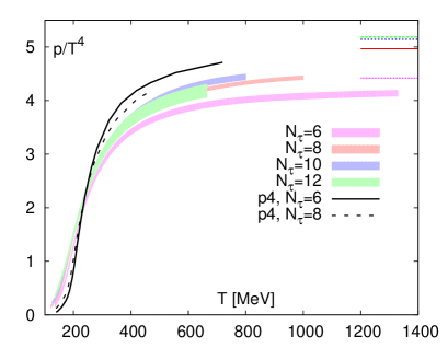
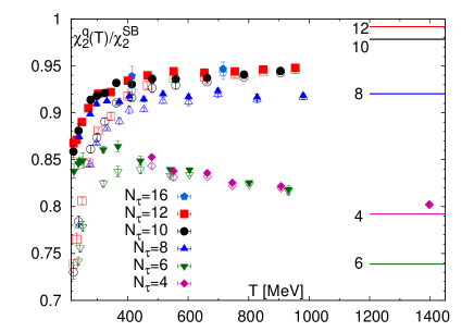
These considerations open up four different approaches to obtain a continuum result for the pressure. First, we may follow [5] and obtain the continuum limit of the trace anomaly and then obtain the continuum pressure via the integral method. Second, we may use the integral method at finite $N_{\tau}$ to obtain the pressure and extrapolate the pressure at fixed temperature to the continuum limit using the appropriate parameterizations of the cutoff effects as discussed in the preceding paragraphs. For an intermediate temperature window, $200\,{\rm MeV}<T<400\,{\rm MeV}$, the picture is less clear and cutoff effects can be described by $1/N_{\tau}^{2}$, $1/N_{\tau}^{4}$ or combinations thereof. Continuum results for either parameterization are consistent within errors in this window, although the continuum limit for $1/N_{\tau}^{2}$ form is slightly higher and the continuum limit for the fits with combined form has large uncertainties due to having only one degree of freedom. We consider the differences as a measure of the systematic uncertainty and use the continuum result for $1/N_{\tau}^{4}$ form as our central value. We double the corresponding statistical error in this window, since this is numerically even more conservative than adding the systematic error in quadrature. For temperatures above $T>670\,{\rm MeV}$ only data with $N_{\tau}\leq 10$ is available and we may consistently extrapolate with controlled uncertainties using the same form. Above $T>800\,{\rm MeV}$ we have only $N_{\tau}\leq 8$ and cannot control the uncertainty of an extrapolation, but provide only a continuum estimate. For $T\approx 800\,{\rm MeV}$ a tentative extrapolation using only $N_{\tau}\leq 8$ yields within errors the same coefficients as an extrapolation using $N_{\tau}\leq 10$. Thus, the continuum estimate seems to be on rather solid ground. This is not completely surprising, since we expect that the coefficients have only a mild temperature dependence due to the logarithmic running of the coupling. In the same spirit, we use the coefficient of $1/N_{\tau}^{4}$ at $T=1\,{\rm GeV}$ to estimate the correction for the pressure with $N_{\tau}=6$ at higher temperatures, up to $T=1.33\,{\rm GeV}$. Third, we may use our knowledge of the cutoff dependence of the QNS to correct for the discretization errors in the pressure. In the weak-coupling picture, the pressure can be written as a sum of quark and gluon pressures $p^{q}$ and $p^{g}$, where the latter has only negligible cutoff effects for an improved gauge action. Then we may assume that the cutoff dependence is completely carried by $p^{q}$, which is dominated by the light quarks, and that it ought to be similar to the cutoff dependence of the second order light QNS $\chi^{l}_{2}$. Finally, we may assume that the continuum limit of $p^{q}$ at high temperatures can be estimated using the rescaled ideal quark gas pressure $p^{q}_{\rm id}$. On the grounds of these considerations, we may develop a scheme for removing the discretization errors of the pressure by using the known results for QNS,

$$p(T)=p(T,N_{\tau})+p^{q}(T)\left(1-\frac{p^{q}(T,N_{\tau})}{p^{q}(T)}\right), \frac{p^{q}(T,N_{\tau})}{p^{q}(T)}\simeq\frac{\chi^{l}_{2}(T,N_{\tau})}{\chi^{l}_{2}(T)},\quad p^{q}(T)\approx 0.85p^{q}_{\rm id}(T).$$ (9)

The advantage of determining corrections from using QNS is that these calculations do not rely on the availability of ensembles at zero temperature with the same parameters. As such, it is considerably cheaper to determine the discretization errors of $\chi^{q}_{2n}$ than for the pressure.

We use the second and third approaches to determine the continuum limit and results that are corrected for cutoff effects up to $T=1.33\,{\rm GeV}$. In Fig. 6 we show these results together with results obtained with p4 action [1] that have been subjected to the same correction approach using corresponding QNS results with p4 action [17]. We interpret this as a validation of the correction procedure that the corrected results with different actions approach the same continuum limit from opposite sides, cf. Fig. 5, and are consistent for $T\gtrsim 400\,{\rm MeV}$ with $N_{\tau}\geq 8$. We note that our continuum result for $T=500\,{\rm MeV}$ is one and a half standard errors larger than the 2+1 flavor result for stout action [4] and agrees well with the previous result for HISQ action [5], although our result has significantly smaller errors.

Figure 6: Left: The pressure calculated with HISQ action for different $N_{\tau}$ and corrected for cutoff effects. The filled squares are the continuum limit of the pressure. For comparison we also plot corrected results with p4 action. Right: The high temperature continuum estimate (open circles) is consistent with the continuum limit and the corrected pressure even without the conservatively enlarged errors.

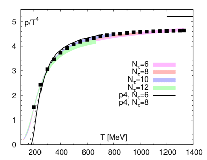
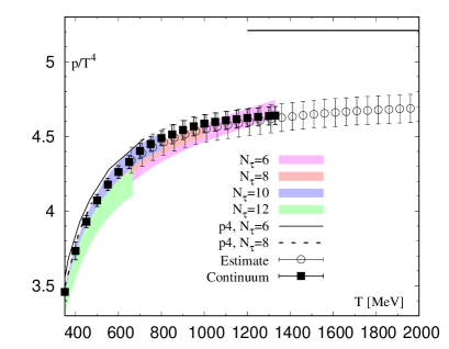
Eventually this is still not sufficient for reaching the highest temperatures $T\approx 2\,{\rm GeV}$ and we need a fourth approach. Hence, we use the first approach to obtain a continuum estimate for $T>1.33\,{\rm GeV}$. Recalling that discretization errors in the trace anomaly with $N_{\tau}\geq 8$ are small for $T>300\,{\rm MeV}$, we obtain a continuum estimate for $\Theta^{\mu\mu}$ by performing a spline interpolation of these data for $T\geq 300\,{\rm MeV}$. Comparison of this continuum estimate and the data with $N_{\tau}=6$ or $N_{\tau}=4$ reveals that these are in the temperature window $800\,{\rm MeV}<T<1\,{\rm GeV}$ smaller by a factor $1.4$ or $1.2$ respectively. Assuming a mild temperature dependence for the trace anomaly at high temperatures as suggested by the weak-coupling limit, we use the same rescaling factors $1.4$ or $1.2$ respectively to estimate corrected results for the trace anomaly from the data with $N_{\tau}=6$ or $N_{\tau}=4$. We then perform a combined spline interpolation of the trace anomaly with $N_{\tau}\geq 8$ for $T\geq 400\,{\rm MeV}$ and the corrected data with $N_{\tau}=6$ or $N_{\tau}=4$ for $T>1\,{\rm GeV}$, where we assign a 40% or 20% systematic error to these corrected data to be conservative. Finally we apply the integral method to this continuum estimate and fix the reference point through the continuum limit of the pressure at $T=660\,{\rm MeV}$. In order to be sufficiently conservative we double the errors of this continuum estimate for the pressure and show it in the right panel of Fig. 6. We stress that none of these error enlargements are necessary in order to obtain full consistency with the continuum limit or the QNS corrected lattice data over the whole common temperature range.

5 Comparison to weak coupling

Armed with the continuum result developed throughout the last section we embark on a comparison to the weak-coupling calculations.

Figure 7: The comparison of the lattice data for the trace anomaly with HTL perturbation theory (red) and EQCD (green) each shown with a line ($\mu=2\pi T$) and a band ($\pi T$ to $4\pi T$). Data with $N_{\tau}=6$ and $4$ for $T>1\,{\rm GeV}$ have been rescaled by $1.4$ and $1.2$, respectively.

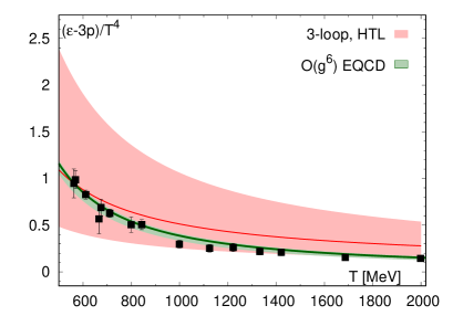
In Fig. 7 we show the lattice data for the trace anomaly, where data with $N_{\tau}=6$ or $4$ have been corrected, see the discussion in Sec. 4. We show the data together with analytic results obtained using hard thermal loop (HTL) perturbation theory at three loop [11] and dimensionally reduced effective field theory, namely the electrostatic QCD (EQCD) at order $\mathcal{O}(g^{6})$ [10]. The uncertainty band of the weak-coupling results are due to variation of the resummation scale $\mu$. We see fair agreement between the different calculations. In Fig. 8, we compare the lattice result for the pressure and entropy density $s=\partial p/\partial T$ to the weak-coupling calculations.

Figure 8: The pressure (left) and the entropy density (right) at high temperatures compared to weak-coupling results. The filled or open symbols are the continuum limit (second approach in Sec. 4), or the continuum estimate (fourth approach in Sec. 4). We show the HTL [11] (red) and EQCD [10] (green) results each with a line ($\mu=2\pi T$) and a band ($\pi T$ to $4\pi T$). For the entropy density the blue band corresponds to the resummed calculation in next-to-leading log approximation (NLA) [18].

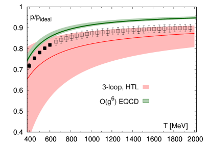
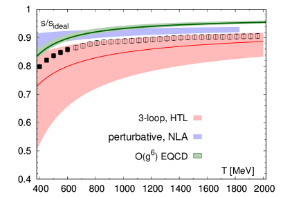
Our result is higher than the central value of the HTL result by about one sigma, but still covered by its scale uncertainty, and a few percent lower than the EQCD prediction. We also compare the entropy to the resummed calculation in next-to-leading log approximation (NLA) [18], which is higher than our result, but consistent within uncertainties for $T>1.3\,{\rm GeV}$. From our comparison it is evident that the presented lattice data are sufficiently precise in order to determine through a comparison with weak-coupling results, whether the thermodynamics of the quark-gluon plasma can be understood in terms of the weak-coupling picture in the given temperature range.

6 Conclusions

We have extended the calculation of the 2+1 flavor QCD Equation of State with the HISQ action to higher temperatures. In order to extend the previous result to higher temperatures we have used gauge ensembles with a light sea quark mass $m_{l}=m_{s}/5$ and demonstrated that the quark mass dependence of the trace anomaly is covered by the statistical uncertainty for $T>400\,{\rm MeV}$. We have determined the pressure from the trace anomaly using the integral method. At low temperatures, we have used a hadron resonance gas with distorted spectrum as reference and have demonstrated that it can describe the trace anomaly for $T<140\,{\rm MeV}$. We have studied the cutoff dependence of the pressure at low and high temperatures and extrapolated the pressure to the continuum limit. Moreover, we have developed a correction scheme for the cutoff effects in the pressure based on the known cutoff dependence of the quark number susceptibilities and the known weak-coupling limit at high temperatures. We demonstrated the validity of this correction scheme by applying it to results with the HISQ and p4 actions at finite $N_{\tau}$, which become numerically consistent with the continuum limit after correction. Finally, we have developed another correction scheme for the trace anomaly with $N_{\tau}<8$ at high temperatures, have demonstrated that it agrees with the other results and have extracted a continuum estimate up to $T\approx 2\,{\rm GeV}$. We have compared this estimate including conservative errors to weak-coupling predictions for the trace anomaly, the pressure and the entropy density and find fair agreement at high temperatures. The lattice results for pressure and entropy density are in the middle between the predictions of different weak-coupling calculations.

References

- [1] M. Cheng et al., Phys. Rev. D 77, 014511 (2008) [arXiv:0710.0354 [hep-lat]].
- [2] A. Bazavov et al., Phys. Rev. D 80, 014504 (2009) [arXiv:0903.4379 [hep-lat]].
- [3] S. Borsanyi, G. Endrodi, Z. Fodor, A. Jakovac, S. D. Katz, S. Krieg, C. Ratti and K. K. Szabo, JHEP 1011, 077 (2010) [arXiv:1007.2580 [hep-lat]].
- [4] S. Borsanyi, Z. Fodor, C. Hoelbling, S. D. Katz, S. Krieg and K. K. Szabo, Phys. Lett. B 730, 99 (2014) [arXiv:1309.5258 [hep-lat]].
- [5] A. Bazavov et al. [HotQCD Collaboration], Phys. Rev. D 90, 094503 (2014) [arXiv:1407.6387 [hep-lat]].
- [6] S. Borsanyi et al., Nature 539, no. 7627, 69 (2016) [arXiv:1606.07494 [hep-lat]].
- [7] A. Bazavov, P. Petreczky and J. H. Weber, Phys. Rev. D 97, no. 1, 014510 (2018) [arXiv:1710.05024 [hep-lat]].
- [8] E. Follana et al. [HPQCD and UKQCD Collaborations], Phys. Rev. D 75, 054502 (2007) [hep-lat/0610092].
- [9] A. Bazavov et al. [MILC Collaboration], PoS LATTICE 2013, 154 (2014) [arXiv:1312.5011 [hep-lat]].
- [10] M. Laine and Y. Schroder, Phys. Rev. D 73, 085009 (2006) [hep-ph/0603048].
- [11] N. Haque, A. Bandyopadhyay, J. O. Andersen, M. G. Mustafa, M. Strickland and N. Su, JHEP 1405, 027 (2014) [arXiv:1402.6907 [hep-ph]].
- [12] P. Petreczky and J. H. Weber,
- [13] A. Bazavov et al., Phys. Rev. D 85, 054503 (2012) [arXiv:1111.1710 [hep-lat]].
- [14] A. Bazavov, N. Brambilla, H.-T. Ding, P. Petreczky, H.-P. Schadler, A. Vairo and J. H. Weber, Phys. Rev. D 93, no. 11, 114502 (2016) [arXiv:1603.06637 [hep-lat]].
- [15] A. Bazavov et al. [TUMQCD Collaboration], Phys. Rev. D 98, no. 5, 054511 (2018) [arXiv:1804.10600 [hep-lat]].
- [16] A. Bazavov et al., Phys. Rev. D 88, no. 9, 094021 (2013) [arXiv:1309.2317 [hep-lat]].
- [17] M. Cheng et al., Phys. Rev. D 79, 074505 (2009) [arXiv:0811.1006 [hep-lat]].
- [18] A. Rebhan, hep-ph/0301130.
- [19] MILC collaboration, MILC code, http://www.physics.utah.edu/$∼$detar/milc/.
- [20] R Core Team, R: A Language and Environment for Statistical Computing, https://www.R-project.org.