Dynamics of Potential Vorticity Staircase Evolution and Step Mergers in a Reduced Model of Beta-Plane Turbulence

Abstract

A two-field model of potential vorticity (PV) staircase structure and dynamics relevant to both beta-plane and drift-wave plasma turbulence is studied numerically and analytically. The model evolves averaged PV whose flux is both driven by, and regulates, a potential enstrophy field, $\varepsilon$. The model employs a closure using a mixing length model. Its link to bistability, vital to staircase generation, is analysed and verified by integrating the equations numerically. Long-time staircase evolution consistently manifests a pattern of meta-stable quasi-periodic configurations, lasting for hundreds of time units, yet interspersed with abrupt ($\Delta t\ll 1$) mergers of adjacent steps in the staircase. The mergers occur at the staircase lattice defects where the pattern has not completely relaxed to a strictly periodic solution that can be obtained analytically. Another types of stationary solutions are solitons and kinks in the PV gradient and $\varepsilon$ - profiles. The waiting time between mergers increases strongly as the number of steps in the staircase decreases. This is because of an exponential decrease in inter-step coupling strength with growing spacing. The long-time staircase dynamics is shown numerically be determined by local interaction with adjacent steps. Mergers reveal themselves through the explosive growth of the turbulent PV-flux which, however, abruptly drops to its global constant value once the merger is completed.

I Introduction

Pattern and scale selection are omnipresent problems in the dynamics of fluids and related nonlinear continuum systems. In geophysical fluids, as described by the beta-plane (Prandtl:2270401, ) or quasi-geostrophic equations (pedlosky2013geophysical, ) - the mechanisms of formation and scale selection for arrays of jets or zonal flows (rhines1982homogenization, ) is of particular interest. The jets scale constitutes and emergent scale which often defines the extent of mixing, transport and other important physical phenomena. Beta-plane and quasi-geostrophic systems evolve by the Lagrangian conservation of potential vorticity (PV). The latter is an effective phase space-density which consists of the sum of planetary and fluid pieces. The question of scale selection then is inexorably wrapped up in the evolution of mixing of potential vorticity. Homogeneous mixing - predicted by the Prandtl-Batchelor theorem (Prandtl:2270401, ; pedlosky2013geophysical, ; rhines1982homogenization, ), leads to a uniform PV profile throughout the system with a sharp PV gradient at the boundary. Inhomogeneous mixing – linked to bistability of mixing, multi-scale PV patterns. One of these – a corrugated structure called the potential vorticity staircase – is of particular interest, as it is a long-lived, quasi-stationary pattern of jets. The struggle between homogenization and (homogeneous mixing) and corrugation (inhomogeneous mixing) of PV is central to the dynamics of staircase formation and evolution, which are the foci of this paper.

The turbulent transport and structure formation phenomenon now commonly known as a ’staircase’, was first understood and described by Philips (Phillips72, ). He considered a density profile in the ocean that, being stably stratified overall, occasionally reorganizes itself into layers separated by thin interfaces. The density gradient flattens in the layers and steepens in the interfaces (sheets). Thus, an initially linear density profile becomes ragged, hence the name ’staircase’. An interesting aspect of the Phillips paradigm – by which it can be distinguished from other pattern formation scenarios in (nonlinear) unstable media – is the pre-existing turbulent transport mechanism that is both supported by, and regulates, the gradient. Even if both the gradient and flux are initially homogeneous, a small local steepening (flattening) of the gradient compared with its mean value results in a local turbulence response that further steepens (flattens) the gradient. The profile thus undergoes a kind of corrugation instability. Positive feedback provided by the instability is equivalent to a ’negative diffusivity’ that enhances the profile corrugation instead of smoothing, in contrast to conventional diffusion. The negative diffusion is often interpreted as the descending branch on an “S-curve” in the flux - gradient relation, i.e. a range of $\nabla n$ for which $\delta\Gamma/\delta\left(-\nabla n\right)<0$ (Hinton91, ). The feedback loop operating macroscopically, drives the transport supporting turbulence out of the regions with steep profiles into adjacent regions with flat ones, so as to maintain the constant net flux across the whole structure, which thus settles at a bistable equilibrium.

Apparently, Philips (Phillips72, ) did not seek to present his mechanism as ubiquitous and universally applicable. However, the general principles behind it suggest looking for its applications to other media, where similar positive feedback may occur. For example, instead of negative diffusion, negative viscosity, also resulting from bistability, may generate strong flow shears. Furthermore, mixing of other quantities, such as temperature, potential vorticity or salinity may also be considered. Dritschel and McIntyre (DritMcInt08, ) review and discuss the relation between the following three effects: mixing of potential vorticity, anti-friction effects in horizontal stress, and spontaneous jet formation (Rhines1994, ). Balmforth et al. (Balmforth98, ) elaborate on a mathematical model for staircase dynamics by evolving buoyancy and turbulent energy via two nonlinear diffusion equations, using a $k-\epsilon$ phenomenology while exploiting an amplitude and scale dependent mixing length. In a number of respects, our approach here is along the lines of (Balmforth98, ) but as the model is different, so are the results. More about the relation of the present model to that developed by (Balmforth98, ) can be found in companion papers (Ashourvan2017, ; HahmDiamondTurbTransp2018, ).

Apart from fluid mechanics, a promising area for applications of the staircase concept is plasma transport in magnetic fusion devices, such as tokamaks. The idea of spontaneously formed transport barriers (N.B. A staircase may be regarded as a chain of such barriers.) has attracted significant interest in the fusion community. A transport bifurcation in the fusion context was first observed in the ASDEX Tokamak (Wagner82, ). This L$\to$H transition occurred with the formation of a transport barrier at the tokamak edge, following a (local) transport bifurcation (116_Burrell97, ; ConnorWilsonLH_REV00, ; DiamRev05, ; Garbet08, ; SchmitzPRL2012, ; Tynan2013, ; Gurcan2015, ). Although most of the research on tokamak transport barriers concerned with such edge phenomena, interest in internal transport barriers is also significant (Dif-Pradalier2015PhRv, ; Kosuga2012, ; Dif-Prad2010, ). Without much risk of oversimplification, a staircase may be thought of as a quasiperiodic array of coupled internal transport barriers.

Despite substantial differences in the mechanisms of transport bifurcation and transport barriers in fluids and plasmas, the apparent commonality of the phenomena suggests certain general principles behind transport barrier formation, their subsequent organization into staircases and the prediction of their possible long-time evolution. We pursue these goals by using a simple generic staircase model, recently suggested. In the present paper, we report new results on the following aspects of the staircase phenomenon. These include

1. identification of conditions and the parameter space for staircase formation,

2. the demonstration of staircase persistence by direct numerical integration of the model equations.

3. finding exact analytic steady state solutions, and exploiting these for code verification.

4. the elucidation of staircase dynamics, long time evolution, merger events and the role of domain boundaries. Special attention is focused upon the physics of mergers.

Taken together, these studies elucidate the basic characteristics of $\mathbf{E}\times\mathbf{B}$/quasi-geostrophic staircases.

The plan of the remainder of the paper is as follows. In Sec. II we give a summary of the staircase model developed previously for geostrophic fluids and magnetized plasmas. Sec.III deals with the bistability conditions, boundary conditions and parameter regimes required for the staircase formation. Sec.IV demonstrates staircase formation by direct numerical integration using a collocation method. In Sec. V we present analytic steady state solutions and use them to verify the numerical method. In Sec.VI the step coalescence (merger), long-time dynamics, quasi-equilibrium staircase configuration and accommodation of boundary conditions are discussed. Sec.VII presents discussion and conclusions.

II Staircase model

The staircase model introduced previously, e.g. (Ashourvan2017, ), and applied here to studies of formation and dynamics is relevant to both geostrophic fluids and magnetized plasmas. These two media are known to be similar. The present model is one dimensional. This may appear as a strong limitation, but due to the symmetry of certain flows (e.g., zonal flows in tokamaks) the 1D approximation is in fact suitable for the purposes outlined in the Introduction. Note that useful insights into transport bifurcation observed in tokamaks have been generated by simple 0D models (KimDiamPRL03, ; MDhyst09, ). The gain for numerical calculations from such simplifications outweighs the limitations as it allows much longer integration with sufficient accuracy. As we will see, staircases typically exhibit disparate spatial scales, and evolve very rapidly before they reach an asymptotic quasistationary regime. Moreover, after a long rest such a seemingly steady state staircase may change abruptly by the merger of two adjacent steps into one in a matter of a tiny fraction of the rest time. These aspects of the staircase phenomenon make its studies computationally challenging, so adaptive mesh refinement is clearly the method of choice here (MuirBacoli2004, ). Three-dimensional numerical studies would be prohibitively expensive for an accurate determination of the time asymptotic evolution.

Because of the disparate spatial and time scales discussed above, code verification is particularly important. A comprehensive code verification is possible in 1D in time asymptotic regimes by comparison with exact analytic solutions. Such solutions will be presented below. Finally, the staircase can be a one-dimensional structure by nature, so much can be learned about it in 1D.

The model that we use in this paper is described in detail previously, so we give only a short review. The model is formulated in terms of potential vorticity (PV) of a geostrophic fluid , such as the one on the surface of a rapidly rotating planet, i.e. atmosphere or ocean. This (PV) quantity, $q$, consists of the planetary vorticity (which we take in the $\beta$-plane approximation) and fluid vorticity:

$$q=\beta y+\Delta\psi$$

where $\psi$ is the stream function, and $y$ is a latitudinal coordinate. By taking the curl of the Euler equation and adding a forcing term to its r.h.s. (which we specify later), one can derive the following equation for $q$

$$\frac{\partial q}{\partial t}-\nabla\psi\times\nabla q=\nu\Delta\psi+f$$ (1)

The vector product component perpendicular to the $\beta$-plane is implied here. Next, we decompose $q$ and $\psi$ into a mean and fluctuating parts

$$q=\mbox{$\left\langle q\left(y,t\right)\right\rangle$+$\tilde{q}\left(x,y,t\right)$}$$

with $\tilde{q}=\Delta\tilde{\psi}$ and substitute this decomposition into eq.(1). After separating the $x$-averaged component $Q\equiv\left\langle q\right\rangle$ from its fluctuating counterpart squared (enstrophy) $\varepsilon=\left\langle\tilde{q}^{2}\right\rangle/2$, a familiar closure problem of how to express $\left\langle\nabla\tilde{\psi}\times\nabla\Delta\tilde{\psi}\right\rangle$ through the averaged quantities $\varepsilon$ and $Q$ arises. For fluctuations which are statistically homogeneous in the $x$-direction it is straightforward to obtain the following (Taylor) identity for the $x$-averaged PV flux $\Gamma_{q}$:

$$-\frac{\partial\Gamma_{q}}{\partial y}\equiv\left\langle\nabla\tilde{\psi}\times\nabla\Delta\tilde{\psi}\right\rangle=\frac{\partial^{2}}{\partial y^{2}}\left\langle\frac{\partial\tilde{\psi}}{\partial x}\frac{\partial\tilde{\psi}}{\partial y}\right\rangle.$$

The Taylor identity relates the PV flux to the Reynolds stress. Here, we find it easier to work with PV than with momentum, as PV is locally conserved. By following the closure prescriptions discussed in previous papers, we apply a Fickian Ansatz for the PV flux: $\Gamma_{q}=-D_{e}\partial Q/\partial y$, where $D_{e}\left(\varepsilon,Q_{y}\right)$ is the PV diffusivity. This is assumed to follow a mixing-length hypothesis, $D_{e}\sim l\left|\nabla\tilde{\psi}\right|$, where $l\left(\varepsilon,Q_{y}\right)$ is the mixing length, introduced phenomenologically as:

$$\frac{1}{l^{2}}=\frac{1}{l_{0}^{2}}+\frac{1}{l_{R}^{2}}.$$ (2)

Here, $l_{0}$ is a fixed contribution to the mixing length $l$ that characterizes the turbulence, e.g., the stirring scale, while $l_{R}$ is the Rhines scale (Rhines1975, ) at which dissipation of $\varepsilon$ balances its production, so $l_{R}=l_{R}\left(\varepsilon,Q_{y}\right)$. In turbulent cascades where wave form of energy coexists with turbulent eddies the Rhines scale is where these two intersect, i.e., where $k\tilde{v}\sim\omega_{k}$ (Rhines1975, ). When the turbulent energy inverse cascade reaches this scale, it is intercepted and transported further by waves both in wave-number and configuration space. A macroscopic consequence of this includes structure formation. A somewhat related phenomenon is encountered in the context of “Alfvenization” of MHD cascades (goldr97, ; BeresnLaz2010, ) in the solar wind and interstellar medium, where the “outer scale” energy is ultimately converted by waves into thermal and nonthermal plasma energy.

Returning to eq.(2), there is still considerable freedom in choosing the functional dependence of $l_{R}$ on its arguments. The only dimensionless combination one may form using the variables entering eq.(2) is $l_{0}^{2}Q_{y}^{2}/\varepsilon\equiv l_{0}^{2}/l_{R}^{2}$. So, we may slightly generalize the relation in eq.(2) and write $l_{0}/l=\left(1+l_{0}^{2}Q_{y}^{2}/\varepsilon\right)^{\kappa}$. We choose $\kappa=2$ and will comment on this choice in Sec.III. Replacing the eddy velocity in the Fick’s law by $l_{0}\sqrt{\varepsilon}$ and measuring $y$ in units of $l_{0},$ we can write the averaged Eq.(1) as follows

$$Q_{t}=\partial_{y}\frac{\varepsilon^{1/2}}{\left(1+Q_{y}^{2}/\varepsilon\right)^{2}}Q_{y}+DQ_{yy}$$ (3)

Here we added to the eddy diffusivity (the first term on the rhs), a conventional collisional diffusivity $D$ that may be associated with the molecular viscosity $\nu$ in eq.(1). We prefer to consider it as a modest additive regularization of the turbulent diffusivity, $D$. Applying similar argument to the turbulent part of PV and adding the terms responsible for its production, damping and unstable growth (see (Ashourvan2017, ; HahmDiamondTurbTransp2018, ) for further details), we write an evolution equation for the potential enstrophy $\varepsilon$ as follows:

$$\varepsilon_{t}=\partial_{y}\frac{\varepsilon^{1/2}}{\left(1+Q_{y}^{2}/\varepsilon\right)^{2}}\varepsilon_{y}+D\varepsilon_{yy}+\frac{\varepsilon^{1/2}}{\left(1+Q_{y}^{2}/\varepsilon\right)^{2}}Q_{y}^{2}-\frac{\varepsilon^{3/2}}{\varepsilon_{0}}+\gamma\sqrt{\varepsilon}$$ (4)

For the purposes of regularization, we use the same background diffusivity $D$ as in eq.(3) (see also below), $\gamma$ is the strength of the forcing, while $\varepsilon_{0}$ quantifies the nonlinear damping of the enstrophy. Apart from these three parameters, the problem depends on the domain size in $y$- direction. Let us measure it in the units of $l_{0}$ and denote by $L.$ Altogether, the system thus depends on four parameters ($D,\varepsilon_{0},\gamma$ and $L$), of which one can be removed by re-scaling the variables. This reduction is, in fact, crucial to the search for staircase solutions, as they occupy a small domain in parameter space. So, by replacing

$$\varepsilon\to\gamma\varepsilon,\;\;\;Q\to\sqrt{\gamma}LQ,\;\;\;y\to Ly,\;\;\;t\to\gamma^{-1/2}L^{2}t$$ (5)

eqs.(3) and (4) transform to the following system

$$Q_{t}=\partial_{y}\frac{\varepsilon^{1/2}}{\left(1+Q_{y}^{2}/\varepsilon\right)^{2}}Q_{y}+DQ_{yy}$$ (6)

$$\varepsilon_{t}=\partial_{y}\frac{\varepsilon^{1/2}}{\left(1+Q_{y}^{2}/\varepsilon\right)^{2}}\varepsilon_{y}+D\varepsilon_{yy}+L^{2}\left\{\frac{Q_{y}^{2}}{\left(1+Q_{y}^{2}/\varepsilon\right)^{2}}-\frac{\varepsilon}{\varepsilon_{0}}+1\right\}\varepsilon^{1/2}$$ (7)

and the integration domain is now $y\in\left[0,1\right]$. These are strongly nonlinear driven/damped parabolic equations possessing numerous stationary and time-dependent solutions. In the next section, we discuss the strategy of our search for the solutions with required staircase properties. To conclude this section, we consider the total enstrophy budget by introducing this quantity as

$$\mathcal{E}\equiv\intop_{0}^{1}\left(Q^{2}/2+\varepsilon/L^{2}\right)dy.$$

From eqs.(6) and (7), we obtain

$$\frac{d}{dt}\mathcal{E}=\intop_{0}^{1}\sqrt{\varepsilon}\left(1-\frac{\varepsilon}{\varepsilon_{0}}\right)dy+\left.\frac{\sqrt{\varepsilon}\left(\varepsilon_{y}/L^{2}+QQ_{y}\right)}{\left(1+Q_{y}^{2}/\varepsilon\right)^{2}}\right|_{0}^{1}-D\left(\intop_{0}^{1}Q_{y}^{2}dy+\left.QQ_{y}\right|_{0}^{1}\right)$$

It is seen that the volumetric enstrophy production due to the instability (first term under the first integral) can be balanced by the nonlinear damping (second term under the integral). The possible enstrophy leak through the boundaries (second term) and small diffusive dissipation can also be compensated by adjusting the nonlinear dissipation rate, $\propto\varepsilon_{0}^{-1}$.

III Staircase Prerequisites

A numerical integration of eqs.(6-7), if not thoroughly planned, shows that staircases (SC) are not ubiquitous solutions that arise from almost any randomly chosen set of parameters and initial conditions. On the contrary, one needs to search for them carefully in a multidimensional parameter space. However, as we will see from the sequel, once the appropriate corner in the parameter space is located, the SC solutions arise as remarkably robust asymptotic attractors of the system given by eqs.(6-7). Apart from the three parameters directly entering these equations ($D,L,\varepsilon_{0}$), two or three additional parameters enter from the boundary conditions for $Q$ and $\varepsilon$, depending on assumptions, discussed briefly below.

First, throughout this paper we impose Dirichlet boundary conditions but fix a PV contrast across the domain, thus maintaining a constant average flux. Specifically, we assume a SC structure to form in a limited $y$-domain (in our variables $y\in\left[0,1\right]$). On each side of this domain a stationary level of $\varepsilon$ is maintained, which in most of the cases considered in this paper is the same: $\varepsilon\left(0,1\right)=\varepsilon_{{\rm B}}$. This reduces the total number of parameters by one. Next, the PV, $Q$, is determined up to an arbitrary constant, so we fix its value on one end, $Q\left(0\right)=0$. Then we set $Q\left(1\right)=Q_{{\rm B}}$, so the enstrophy inside the SC is driven by the gradient $Q_{y}$ (the first term in braces in eq.[7], with $\left\langle Q_{y}\right\rangle=Q_{{\rm B}}$), in addition to the constant drive given by the very last term in the braces. At a minimum, we thus have a 5D parameters space to search in for a SC solution. Clearly, we need directions for our search.

In rough terms, a SC structure described in Sec.I may result from the loss of stability of a ground state solution of eqs.(6-7) characterized by the constant values $\varepsilon=\varepsilon_{B}$ and $Q_{y}=Q_{B}$ that annihilate the term in braces in eq.(7). Then, nonlinear saturation of the instability may possibly lead to a (quasi)stationary SC solution. A generic paradigm here is bistability, where apart from the unstable ground state, there exist two stable steady states. The system jumps to one of these when the ground state becomes unstable. To explain the conditions for this scenario, let us denote the enstrophy production-dissipation term in braces on the r.h.s. of eq.(7) as

$$R\equiv\frac{Q_{y}^{2}}{\left(1+Q_{y}^{2}/\varepsilon\right)^{2}}-\frac{\varepsilon}{\varepsilon_{0}}+1$$ (8)

A SC, particularly the one with a large number of steps, evidently requires $L\gg 1$. Otherwise, the diffusive terms in eqs.(6-7) will dominate, thus driving the $\varepsilon$ and $Q_{y}$ profiles to constants. Therefore, assuming $\partial_{t}Q\approx 0$ and $L\to\infty$, it follows that $R\to 0$. Thus, with some reservations discussed below, eq.(7) can be written for $L\gg 1$ as

$$\varepsilon_{t}=L^{2}\sqrt{\varepsilon}R\left(\varepsilon,Q_{y}\right)$$ (9)

It should be noted here that (as $L\gg 1$) the first two terms on the r.h.s. of eq.(7) are small terms, with higher derivative discarded in eq.(9). Boundary layers are expected between the states with high and low values of $\varepsilon$ associated with two stable fixed points in eq.(9). Also note that $Q_{y}$ may (and will) jump between these fixed points along with $\varepsilon$, but the jump description requires treating the neglected higher derivative terms that will be taken into account in Sec.V. We will call the thin regions over which $\varepsilon$ and $Q_{y}$ jump, the ’corners’, as they appear as such in the $Q\left(y\right)$ profile (see Fig.3). A region of flat $Q$ (large $\varepsilon$) attached to the corner on one side we call a ’step’. A contrasting region, where $Q$ is steep (small $\varepsilon),$ we call a ’shear layer’ or ’jump’. In essence, such structure corresponds well to the SC phenomenon, since the corners between the shear layers and steps, as envisioned by Phillips (Phillips72, ), are simply the internal boundary layers.

Figure 1: Enstrophy production-dissipation term $R$ in eqs.(7,8) as a function of enstrophy $\varepsilon$, shown for a fixed mean vorticity gradient $Q_{y}=35$ and $\varepsilon_{0}=3.55$.

The conditions for generating the SC structures described above can be approached assuming constant local enstrophy and vorticity gradient $\varepsilon,$$Q_{y}\equiv const$. Here, we constrain the parameters in the driving term $R$ to have a bistable form shown in Fig.1. In this case, the alternating layers correspond to jumps between two stable equilibria (fixed points), over an unstable one. Of course, one can directly solve the cubic relation $R=0$ for, e.g., $\varepsilon$ as a function of $Q_{y}$ and $\varepsilon_{0}$, thus determining conditions for the three roots to exist. However, this approach is algebraically tedious, so we take a different route. First, denote $\xi\equiv\varepsilon/Q_{y}^{2}=l_{R}^{2}$ and rewrite the equation $R=0$ after dividing it by $Q_{y}^{2}$

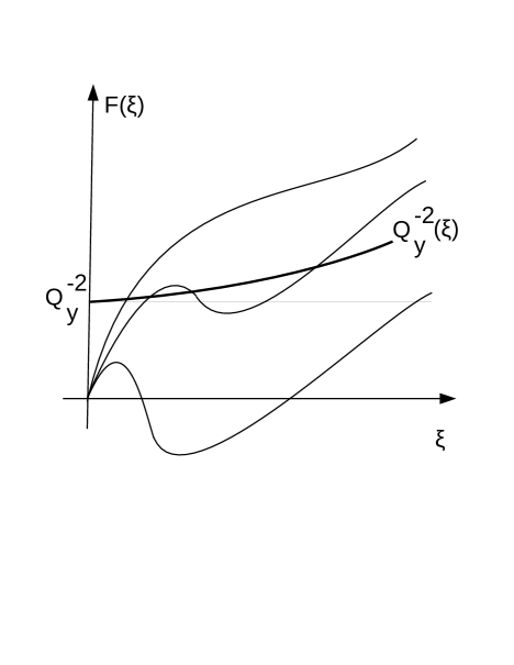
Figure 2: Left-hand side of eq.(10), $F\left(\xi\right),$ schematically drawn for three different values of parameter $\varepsilon_{0}$.

$$F\left(\xi\right)\equiv\frac{\xi}{\varepsilon_{0}}-\frac{\xi^{2}}{\left(1+\xi\right)^{2}}=\frac{1}{Q_{y}^{2}}$$ (10)

In this form, the variables $\xi$ and $Q_{y}$ are separated while $\varepsilon_{0}$ is considered as a constant parameter. For this equation to have three real roots (the scenario of bistability), the value $1/Q_{y}^{2}$ must fall between the local extrema of $F\left(\xi\right)$, provided that they exist, i.e.:

Figure 3: Generation of a one-step profile out of an unstable ground state superposed by small perturbations (short-dash lines). Perturbations are low-amplitude, so short scales are not seen clearly in the initial profile but they do not affect the profile evolution significantly. The Dirichlet boundary conditions are applied for $Q$ and $\varepsilon$ at both boundaries. The other parameters are $\varepsilon_{0}$=3.8, $L^{2}=2.3\cdot 10^{3}$, $D=1.5$, the boundary conditions can be read from the plots.

$$F_{{\rm min}}<Q_{y}^{-2}<F_{{\rm max}}.$$

(see Fig.2). Denoting the points of extrema by $\xi_{0,1}$, this constraint can be written, using eq.(10) as follows

$$\xi_{1}\left(1-\xi_{1}\right)<\frac{2\varepsilon_{0}}{Q_{y}^{2}}<\xi_{0}\left(1-\xi_{0}\right)$$ (11)

Note that the left term of this inequality becomes negative for sufficiently large $\varepsilon_{0}$ (lower curve in Fig.2). The two extremal points of $F\left(\xi\right),$ $\xi_{0}<\xi_{1}$ , where $F^{\prime}\left(\xi_{0,1}\right)=0,$ are also to be found from a cubic equation, but this equation is much simpler than the original one, given by eq.(10). The requirement for the two isolated roots $\xi_{0,1}$ to exist is $\varepsilon_{0}$>27/8 (Appendix A). This condition proved very useful in the search for a SC regime. However, the latter is not precise in that $Q_{y}$ and $\xi$ also change during the transition from one stable state to the other. In fact, one can easily determine $Q_{y}\left(\xi\right)$ variation by assuming that it changes in space but remains stationary. This assumption relates $Q_{y}$ to $\xi$ by the constant diffusive flux in eq.(6). Denoting the flux of $Q$ by $b$ (see Appendix A and eq.[13] below) we obtain the following relation for $Q_{y}$ to be used in the constraint (11) for connecting the two stable roots of eq.(10)

$$\frac{1}{Q_{y}}=\frac{D}{2b}+\sqrt{\frac{D^{2}}{4b^{2}}+\frac{\xi^{5/2}}{b\left(1+\xi\right)^{2}}}$$ (12)

By substituting the last relation into the rhs of eq.(10), one can solve it for $\xi$ in terms of the three parameters $\varepsilon_{0},D,$ and $b$. For certain values of these parameters, three isolated roots are possible, of which the largest and the smallest correspond to neighboring layers in a staircase solution, or to the two stable roots of the truncated equation (9). The intermediate root is unstable. For practical reasons, instead of locating all three roots, we constrain the parameter space by the simple analytic formulae (11) and ( 20). They provide a range of $Q_{y}$ for possible staircase solutions in terms of $\varepsilon_{0}$. The region in the $\varepsilon_{0},Q_{y}$ plane, where to look for the staircase numerically, is shown in Fig.4.

Figure 4: Part of parameter space in variables $\varepsilon_{0},Q_{y}$ where the SC solutions are possible.

It follows that a stationary staircase structure is a quasi-periodic sequence of regions with alternating upper and lower stable $\varepsilon$ values in Fig.1. As we will see in the sequel, time-asymptotically this solution can be calculated analytically. The exact analytic solution provides both a guidance in exploring the time-dependent regimes and an excellent code verification tool.

In addition to the above guidance, the following consideration has proven useful in search for staircase solutions. As they result from an unstable stationary solution with initially constant $\varepsilon$ and $Q_{y}$, a stability analysis of the full system can be performed. This replaces the local analysis above, based on the zeroes of the function $R\left(\varepsilon\right)$ and signs of its derivatives $R^{\prime}\left(\varepsilon\right)$. This extended analysis, even if it probes only simple perturbations of the type $\propto\exp\left(iky-i\omega t\right)$, is rather tedious. It is also more restrictive, as it does not capture the bistable state described earlier. So, we do not reproduce the linear analysis here. However, a broader insight into the parameter choice for obtaining the staircase solution has been gained from this analysis. As mentioned earlier, the mixing length scaling in eq.(2) can be written more generally as $l_{0}^{2}/l^{2}=\left(1+l_{0}^{2}/l_{R}^{2}\right)^{\kappa}$ and the stability analysis can be performed for this, more general form of the mixing length. Our particular choice $\kappa=2$ in the model equations (6-7) was precisely dictated by the instability condition for a steady state solution with constant $\varepsilon$ and $Q_{y}$. At the same time, even without performing such a stability analysis of the full system, an alternative choice $\kappa=1$ instead of $\kappa=2$ may be shown to be inconsistent with SC solutions. Namely, the denominator of the first term in $R$ from eq.(8) is simply $1+Q_{y}^{2}/\varepsilon$ in this case. Therefore, the function $R\left(\varepsilon\right)$ has only one positive stable root at which $R^{\prime}\left(\varepsilon\right)<0$. Hence, no bistability occurs, so no staircase forms!

Another important aspect of the stability analysis regards the possible number of steps in the structure. Indeed, by contrast to the above discussed local bistability based on eq.(9) (in essence, a $k\to 0$ limit), the standard linear analysis assumes perturbations of the form $\propto\exp\left(-i\omega t+iky\right)$. The small scales are damped, as $\Im\omega\simeq-k^{2}$, but the growth rate turns positive for small $k$ and sufficiently large $L$. Thus, there must be a maximum unstable $k$, and possibly even maximum $\Im\omega\left(k\right)$, depending on the boundary conditions. This $k$ sets the number of steps in the staircase! However, as numerical integration shows, this initial number (being also somewhat sensitive to the initial conditions) quickly relaxes to a smaller number of steps, as the staircase grows to a nonlinear level. This quasi-equilibrium staircase configuration and its time evolution are the main focus of our study below.

IV Staircase formation

It follows from the above considerations that the number of steps in a staircase must grow with the parameter $L$. It is thus natural to assume that at some moderate value of $L$, this number can be as small as one. Shown in Fig.3 is a one-step profile generated from an unstable ground state with small scale weak perturbations (short-dash lines) superposed. The initially small scales are quickly damped, and the system evolves to a one-step profile, shown by heavy lines. In Sec.V we will demonstrate that this profile coincides with an exact stationary solution of the system. As it appears to be stable, it must persist indefinitely, thus constituting a single step attractor. The $\varepsilon$ and $Q_{y}$ profiles are symmetric with respect to the mid-plane, as the boundary conditions also are, $\varepsilon\left(0\right)=\varepsilon\left(1\right)$ .

An example of asymmetric profile is shown in Fig.5. In this case, the boundary conditions are different at the left and right boundary, $\varepsilon\left(0\right)\neq\varepsilon\left(1\right)$. Although the system also evolves into a staircase with only one step, this time the step attaches itself to one of the boundaries. The steep part of the $Q$-profile attaches itself to the opposite boundary. A point of special interest associated with this simple configuration is its similarity to the temperature and density distributions in H-mode (high confinement regime) of operation of magnetic fusion confinement devices. The region at the left boundary with a steep gradient of the transported (by turbulence) quantity ($Q$ in this case) is characterized by transport reduction associated with the low turbulence level, ($\varepsilon$ here).

Now that we have demonstrated that a stationary staircase is indeed a strong attractor for the time-dependent system given by eqs.(6-7), it is worthwhile to investigate all possible steady-state solutions analytically. This investigation will be useful in numerical studies of staircase dynamics, presented later in Sec.VI.

Figure 5: The same plots as in Fig.3 but for $L^{2}=900$. Other parameters are the same, except the turbulence level is kept at different levels on right and left boundary. As the mid-plane symmetry is broken, the initially formed profiles propagate to the right boundary. After $t\lesssim 1$, the $Q$-profile relaxes to one step at the right boundary and a shear layer at the left. This configuration persists in time, as the boundary conditions are consistent with a part of periodic stationary solution, Sec.V, that fits into the integration domain.

V Analytic solution for time-asymptotic staircase

Analytical time-asymptotic staircase solutions can be obtained easily. These solutions are also relevant to the staircase dynamics since – as we will see from the numerical studies – a typical multi-step staircase does not change in time, apart from quick merger events. One may refer to it as “meta-stationary”. Between such merger events, the staircase is perfectly described by analytic solutions that we obtain below and compare against numerical solutions in Sec.V.1.

Assuming a steady state, from eq.(6) we deduce

$$\left[\frac{\varepsilon^{1/2}}{\left(1+Q_{y}^{2}/\varepsilon\right)^{2}}+D\right]Q_{y}\equiv b=const$$ (13)

Instead of $Q$ and $y$, it is convenient to use the following two variables as dependent and independent, respectively

$$\psi=\frac{Q_{y}}{\sqrt{\varepsilon}},\;\;\;\eta=\sqrt{2}Ly,$$ (14)

We keep $\varepsilon$ as the second dependent variable. Assuming also $\partial\varepsilon/\partial t=0$, multiplying eq.(7) by a factor $2\varepsilon_{y}/bQ_{y}$ and integrating once in $y$, we arrive at the following first integral of this equation

$$\frac{\varepsilon_{\psi}^{2}}{\psi^{2}\varepsilon}\left(\frac{d\psi}{d\eta}\right)^{2}+W\left(\psi\right)=E=const$$ (15)

where

$$W\left(\psi\right) = \varepsilon-\frac{2D}{3b}\psi\varepsilon^{3/2}+\frac{\varepsilon}{b\psi}\left(1-\frac{\varepsilon}{2\varepsilon_{0}}\right)$$ (16)

$$+ \frac{2D}{3b}\int\varepsilon d\psi+\frac{1}{b}\int\frac{\varepsilon}{\psi^{2}}\left(1-\frac{\varepsilon}{2\varepsilon_{0}}\right)d\psi,$$

$\varepsilon_{\psi}=\partial\varepsilon/\partial\psi$ and $\varepsilon\left(\psi\right)$ can now be written in the following explicit form

$$\varepsilon=\left(1+\psi^{2}\right)^{2}\left[\sqrt{\frac{b}{\psi}+\frac{1}{4}D^{2}\left(1+\psi^{2}\right)^{2}}-\frac{1}{2}D\left(1+\psi^{2}\right)^{2}\right]^{2}$$ (17)

It follows that the first integral in eq.(15) provides the steady state solution of eq.(7) in the form of $\psi\left(\eta\right)$ which can be obtained by inverting the function $\eta\left(\psi\right)$. This in turn, can be derived from eq.(15) by quadrature. Furthermore, using eqs.(14) and (17), one can obtain the steady state solution in original variables, $Q\left(y\right)$ and $\varepsilon\left(y\right)$.

For the purpose of comparison of the solution given by eq.(15) with the asymptotic regime obtained from the numerical integration of eqs.(6-7), we return to the original coordinate $y$ and write the solution in the form of $y=y\left(\psi\right):$

$$y=\frac{1}{\sqrt{2}L}\int\frac{\partial\varepsilon}{\partial\psi}\frac{d\psi}{\psi\sqrt{\varepsilon\left[E-W\left(\psi\right)\right]}}$$ (18)

Apart from an arbitrary constant $y_{0}$, that can always be added to the rhs to adjust the position of the staircase in $y$, the solution $\psi\left(y\right)$ in eq.(18) depends on two further constants, $E$ and $b$. The latter is the flux of $Q$ that enters $W$ in the last expression by virtue of eq.(16). Although $b$ is related to the boundary conditions because of eq.(13), under the Dirichlet boundary conditions employed here $Q_{y}$ is not fixed at the boundaries. Therefore, $b$ becomes constant only when the system reaches a steady (or meta-stationary, as discussed earlier) state. Before such state, presented in eq.(18), is reached $b$ changes in time.

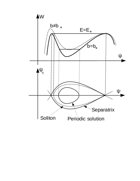
Figure 6: ’Oscillator’s’ pseudo-potential and its phase plane. The top panel shows the function $W\left(\psi,b\right)$ from eq.(15) for the case when two maxima that correspond to two zeros of function $R\left(\varepsilon\right)$ in eq.(8) are at the same value of $W=E_{{\rm max}}.$ The maxima are the same for a specific value of the constant flux $b$ in eq.6. For $E<E_{\max}$ solutions are periodic.

The role of the constants $E$ and $b$ can be elucidated by returning to the first integral in eq.(15) and interpreting it as a constant total energy of a pendulum with a variable mass (coefficient in front of $\psi_{\eta}^{2}$) moving in a potential well $W\left(\psi\right)$. The variable $\psi$ plays the role of a coordinate here while $\eta$ is ’time’. One form of $W\left(\psi\right)$, shown in Fig.6, corresponds to a specific value of $b=b_{*}$ for which the two maxima of $W\left(\psi\right)$ are equal. This is an important case since it admits heteroclinic orbits connecting two hyperbolic points of the ’pendulum’ at a specific value of $E=E_{*}$. The orbits correspond to the two branches of a separatrix shown on the phase plane in Fig.6. These particular values of $b=b_{*}$ and $E=E_{*}$ correspond to an isolated transition from low to high values of $\psi$, when $y$ runs from $-\infty$ to $+\infty$. The original variables $\varepsilon$ and $Q_{y}$ can always be restored unambiguously from $\psi\left(y\right)$ using eqs.(17) and (14). The mirror branch of this orbit corresponds to the reverse transition and fixed points correspond to the two stable roots of the function $R\left(\varepsilon\right)$ introduced in Sec.III and depicted in Fig.1. Clearly, for a heteroclinic orbit to exist the two areas cut by the abscissa from $R\left(\varepsilon\right)$ curve between the stable and two unstable roots must satisfy a certain relation. This is that measured (integrated) in the variable $y$ instead of $\varepsilon$, these areas must be equal, as it follows from the derivation of eq.(15). Using the pendulum analogy again, the heteroclinic orbit connects two unstable equilibria (the two humps on the potential energy profile). Therefore, the accelerating phase of the trajectory must be exactly annihilated by the decelerating phase. This is equivalent to the familiar Maxwell’s construction, illustrated in Fig.7. The Maxwell rule is common for other transition phenomena, both flux and source driven (LebDiam97, ; murray2001mathematical, ; MDtranspBif08, ).

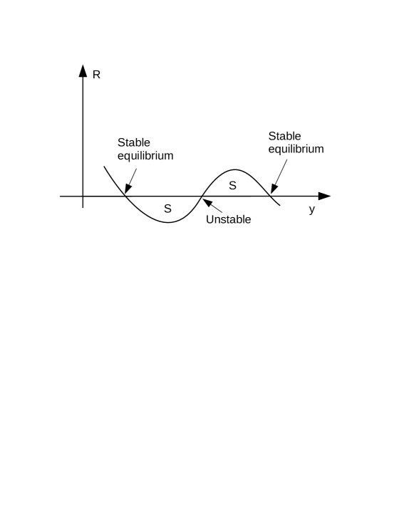
Figure 7: Illustration of a Maxwell transition rule, in a form of the production-dissipation function, $R\left(y\right)$. In order to connect the two stable equilibria, shown in Fig.1, with one heteroclinic orbit, shown in Fig.6, the areas above and below the abscissa must be equal.

For values of parameters $E$ and $b$ other than discussed above, the solutions given by eq.(18) fall in two further categories: (i) strictly periodic solutions corresponding to $E<E_{*}$, while $b$ may or may not remain equal to $b_{*}$, Fig.6, and (ii) soliton type solutions when the orbit is homoclinic, starting and ending at one of the two hyperbolic points. Here $b\neq b_{*}$, $E=E_{*}$, so we have only one hyperbolic fixed point on the orbit. Just as the heteroclinic solution described earlier, this solution also becomes periodic for $E<E_{*}$. The periods of solutions with $E<E_{*}$ can be calculated using eq.(18) as

$$\mathcal{L}\left(E,b\right)=\frac{\sqrt{2}}{L}\int_{\psi_{1}}^{\psi_{2}}\frac{\partial\varepsilon}{\partial\psi}\frac{d\psi}{\psi\sqrt{\varepsilon\left[E-W\left(\psi\right)\right]}}$$ (19)

Here the integral runs between the two turning points obtained from the relation $W\left(\psi\right)=E$. By contrast with compact solutions, i.e. isolated transitions or solitons (which do not ’fit’ into a finite domain), the periodic solutions can be fully described on a $\left[0,1\right]$ segment, provided that $\mathcal{L}<1$. In general, however, and especially when $n\mathcal{L}\neq 1$ with $n=1,2,\dots$, the boundary conditions need to be consistent with parameters $b$ and $E$. We will touch upon this aspect of the solution later.

V.1 Comparison of time-asymptotic numerical solutions with the analysis

A comparison of the analytic solutions given above with those obtained numerically serves several purposes. Firstly, it verifies the code’s accuracy and convergence, while establishing its limitations. The latter is particularly important in view of the time- and space-scale disparities inherent in this problem. Secondly, it verifies that the analytic solutions are indeed the attractors for the time-dependent solutions. In addition, the numerical integration delineates the basins of attraction of these analytic solutions. Finally, such comparison gives insight about a possible evolution of the system beyond the accessible integration time.

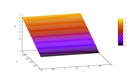
Figure 8: Merger of steps shown as a surface plot of the mean vorticity $Q\left(t,x\right)$ with the Dirichlet boundary conditions, $\Delta Q=6.2,$ between the right and left boundary, $\varepsilon_{0}=10.38$, $L^{2}=1.5\cdot 10^{5},$ $D=1.7$. Initially, as many as 12 steps are formed but very rapidly ($t\lesssim 0.1)$ they merge to 7. The 7-step configuration lasts with no numerically significant changes up to the moment $t\approx 2$ when two shear layers near the walls disappear and the edge steps merge into respective walls. The remaining staircase structure persists up to $t\simeq 100$ when the two edge steps merge with their neighbors.

The latter aspect is crucial in that the time dependent solutions typically show a long rest - transition burst alternation. Fig.8 shows an example of such behavior. After quick ($t\lesssim 0.1$) mergers of the ten out of the twelve initially formed steps ($10\to 5$), the systems sits at the state of seven remaining steps for a long time, $t\approx 2$. Moreover, at this time the staircase merely accommodates the boundary conditions by attaching each of the two edge steps to the respective boundary, Fig.8. In the next section, a case of much longer rest will be presented. We will also take a closer look at a typical merger event. Without analytic predictions, it is difficult, if not impossible, to tell whether the long rests are genuine attractors of the system or the next merger is to be expected. Also, if yes, then what determines the waiting time? Conversely, if a merger occurs after a long rest period– during which the profile agrees with one of the stationary analytic solutions– one may consider such a merger as a spurious effect of accumulated round-off errors.

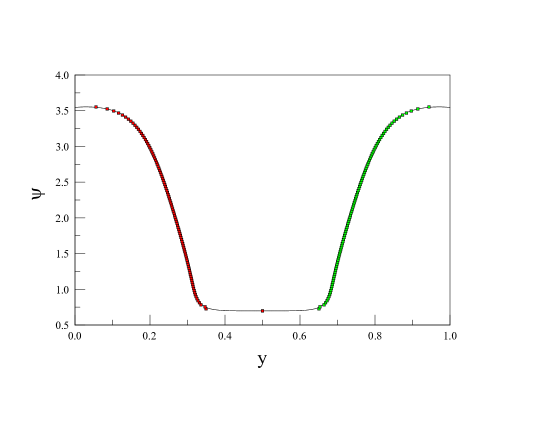
Figure 9: Numerical solution of eqs.(6-7) in long-time asymptotic regime, shown with the solid line. The parameters are the same as in Fig.3. Exact analytic solution represented by the two branches of $y\left(\psi\right)$ in eq.(18), shown with red and green squares.

For the purpose of comparison with numerical solutions, the constants $b$ and $E$ – which an analytic solution depends upon – should be calculated using boundary conditions imposed on the numerical solutions. More practically and equivalently, we extract them directly from the numerical solution already shown in Fig.3. An exact analytic solution, plotted using eq.(18), is compared to this numerical solution in Fig.9. Given the parameters $b$ and $E$, the analytic solution is obtained by a simple tabulation of the integral in eq.(18), even without regularization of the integrand singularities at $W=E$. This explains a non-uniform, coarse sampling, as well as a minor deviation of one point next to the minimum of $\psi\left(y\right)$ from the numerical curve. The extrema of $\psi\left(y\right)$ obviously correspond to the algebraic ($E<E_{*}$) or logarithmic ($E=E_{*})$ singularities of $y\left(\psi\right)$ .

The parameters and boundary conditions for the run in Fig.9 are such that the entire profile spans slightly more than one period of the respective analytic solution, $\mathcal{L}\lesssim 1$. Furthermore, in the asymptotic state shown in the figure, the flux $b$ is constant throughout the integration domain to within the code accuracy, so the solution is indeed steady. Note that we varied the code error tolerance between $10^{-8}-10^{-6}$ (see (MuirBacoli2004, ) for the algorithm’s description and further references) without sizable effects on convergence, up to $t\sim 100$. Further details on the comparison of analytical and numerical solutions are given in Appendix 2.

These results – and particularly the perfect agreement between the overall analytic and numerical solutions along with the code convergence (insensitivity to the error tolerance) – increase our confidence that the code accurately describes the evolution of the staircase system in time.

VI Staircase merger events

The purpose of this section is to connect staircase mergers with the analytic properties discussed in the previous section. Within the range of parameters outlined in Sec.III, the numerical integration of eqs.(6-7) consistently demonstrates the following evolution: long meta-stationary periods interspersed by quick staircase mergers. During these periods, the staircase configuration does not change in any noticeable way, and is accurately described by analytic solutions obtained in the preceding section. Natural questions then are: what causes the next merger, and does it become final – beyond which the staircase configuration will stay unchanged. Here the word ’unchanged’ should be taken with caution, as our simulations clearly show that nearly perfectly stationary staircase configurations lasting for $t\gtrsim 100$ do merge eventually, and over times $t\lesssim 0.1$. Recall that time here is given in units of $L^{2}/\sqrt{\gamma}$, eqs.(4) and (5). Despite these remarkably disparate time scales, the answer that we find below is at least consistent with the analytic solutions.

Figure 10: Typical profile of $\nabla Q$ (or $Q_{y}$) where FWHM (full width at half maximum) characterizes the width of shear layers (humps) and steps (troughs) on the plot. Here $D=1.5,\;\;L^{2}=10^{5},\;\quad\varepsilon_{0}=3.7915,\;\;Q\left(1\right)=6.2,\;\;\varepsilon\left(0,1\right)=10.38$

Typically, a quasi-stationary staircase forms very quickly ($t\ll 1)$ with $n$ steps separated by shear layers exhibiting a significantly steeper gradient of the mean vorticity $Q_{y}$ also with suppressed enstrophy level, $\varepsilon$. The number $n$ is determined by the maximum growth rate (similarly to the results of (Balmforth98, ), see also Sec.III) and partly by the initial conditions. Then, over a somewhat longer time (but still $t<0.1$), most – except the boundary-attached – steps merge with their neighbors. So, the total number of steps becomes $\approx n/2$. This phase of the staircase evolution is typically similar to that shown in Fig.11 (which shows a time history behind the $Q_{y}$ -profile shown in Fig.10). After this initial phase the staircase persists for a much longer time. It is clear from the surface plot of the $Q$-flux that it grows rapidly, and deviates strongly from its globally constant value precisely at the merger locations.

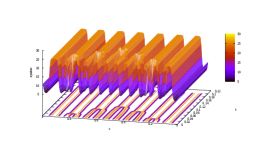
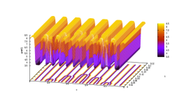
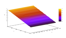
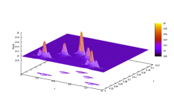
Figure 11: Time history and details of the staircase merger sequence that led to the profile shown in Fig.10. The top two panels show the enstrophy $\varepsilon$ and $Q_{y}$ , while the bottom panels show the mean potential vorticity $Q$ and its flux given by eq.(13). The early relaxation phase $t\lesssim 0.01$ is removed from the plots to emphasize the flux strong variation during the later staircase mergers.

The further fate of a quasi-stationary staircase depends on the following factors. One factor is the proximity of the staircase to the periodic solution described in Sec.V. The portions of the staircase profile that are periodic do not merge, consistent with the analytic solutions. As we have seen, all stationary solutions are exhausted by either periodic or compact (solitary or kink type) solutions . Therefore, the periodic segments of the staircase tend to be steady. An example of such a staircase is shown in Fig.8. After quick initial mergers, this staircase remains periodic in its interior and only the edge regions deviate from spatial periodicity. Here, the second factor that influences the evolution of a staircase enters. This is the boundary effect. Indeed, as we discussed in Sec.V.1, at $t\approx 2$ the edge shear layers disappear and the edge steps attach themselves to the boundaries. An inspection of the $Q$-flux shows that it remains constant in the interior where the staircase is periodic, and it progressively deviates from the constant values near the boundaries. This ultimately results in the boundary accommodation event at $t\approx 2$, after which the flux returns to its global average. After this event, however, the staircase becomes non-periodic at the edges (edge steps are broader than the central ones). As expected, the edge steps merge with their neighbors, but only at $t\approx 100.$

A different example of a staircase, that is noticeably non-periodic, is shown in Fig.10. Such configurations tend to merge over significantly shorter time, particularly at those locations where the steps or shear layers are close to each other. So, the spacing between the neighboring corners is important for the mergers. These corners separate steps from shear layers. As we know, a single corner with a step and a shear layer on each side makes a stationary structure in an infinite space and is described by a heteroclinic orbit. It approaches exponentially constant values at $\pm\infty$ that characterize the step and the shear layer, respectively. Two neighboring corners, for example, form either an isolated step or isolated shear layer, e.g. Fig.3. Based on Sec.V, this construction does not belong to any type of stationary solution in infinite space. However, if its corners are well separated by a broad step or shear layer, their interaction term is$\sim\exp\left(-L\Delta y\right)\ll 1$, where $\Delta y$ is the distance between the corners and $L\gg 1$ (see SecV and Fig.3). So, broad, well separated steps and layers in a staircase must also persist in time. Typically, when the system relaxes to 4-5, not perfectly periodic steps, the next merger occurs after several hundreds of time units. Integration beyond this time would require a significantly lower error tolerance. Under these circumstances, analytic predictions become much more reliable than numerical ones.

Figure 12: $Q-$ flux as a function of time immediately before and during the merger event near $t\approx 0.09$ at the middle of integration domain at $y=0.5$ shown in Fig.11. For the clarity of representation and a functional fit, shown in Fig.13, the flux is adjusted by subtracting a reference value $F_{B}\approx 13.96088$ which is close to a globally averaged flux.

Staircase steps merge in a rather interesting way. Fig.11 shows a sequence of such mergers of 12 initial steps (see the $Q$-panel). The mergers proceed symmetrically from the boundaries towards the center of the integration domain. This process continues until the mergers converge at the center and the central two steps merge into a bigger step. Here, we concentrate on this last merger by zooming into it in time. The best variable for characterization of the merger is the $Q-$ flux, which is shown in Fig.12 at the point $y=0.5$ as a function of time. The flux remains constant when no mergers occur (constant $b$ in stationary solutions of Sec.V), so we subtract this constant value for clarity and for the purpose of functional fitting below. As seen from the plot, the flux builds up in two distinct phases before it drops abruptly to its averaged value after the merger. The first phase is an initial growth that lasts to about $t\approx 0.065$. The flux increase remains relatively small, $\lesssim 0.01$. The second phase is clearly explosive and can be accurately fit by the following function, Fig.13

$$F=F_{0}+B/\left(t_{0}-t\right)^{\alpha}$$

with $t_{0}\approx 0.0863$, $B\approx 0.000806$, $\alpha\approx 0.879$, and a residual flux $F_{0}\approx-0.0171$ . Note that apart from this last constant, the background value $F_{B}\approx 13.9609$ has been subtracted from the total flux. By contrast with the initial phase, the local flux excess grows to a value $\gtrsim 1$ before the merger occurs, and the total flux then drops abruptly to its background value.

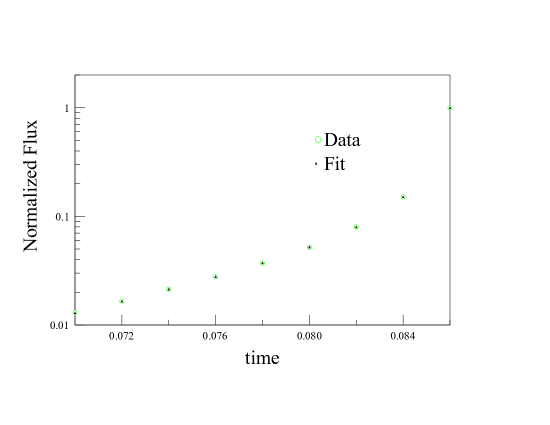
Figure 13: Fit of the flux in its self-similar phase of evolution for $0.070<t<0.086$. The fit is given by $F=F_{0}+B/\left(t_{0}-t\right)^{\alpha}$ with $t_{0}\approx 0.0863$, $B\approx 0.000806$, $\alpha\approx 0.879$, subtracted background $F_{B}\approx 13.96088$, a residual flux constant $F_{0}\approx-0.0171$.

VII conclusion

The Phillips’s staircase (Phillips72, ) has long since outgrown its original context. Indeed, it is of general interest as an outcome of the nonlinear scale and pattern selection processes in systems with an homogeneously mixed conserved density. The present paper is devoted to numerical studies and analysis of a limiting case of new staircase model recently introduced in (Ashourvan2017, ), in the context of geostrophic fluids and magnetized plasmas. It evolves the potential vorticity (PV) and potential enstrophy with a versatile model of mixing set by the Rhine-scale. The model controls enstrophy production by the PV gradient, additional independent pumping, and nonlinear damping. These system properties render it bistable, which is the key to staircase formation.

The main results of the current investigation of this model can be summarized as follows:

1. parameter regimes and mixing length scalings in which the staircases occur are analytically constrained to satisfy: $l_{0}^{2}/l^{2}=\left(1+l_{0}^{2}/l_{R}^{2}\right)^{\kappa}$, $\kappa>1$, $l_{R}$ is the Rhines scale $l_{R}^{2}=\varepsilon/Q_{y}^{2}$

2. staircase formation, their properties and stability were studied numerically, for differing parameters and boundary conditions

3. analytic solutions for steady state staircase configurations are obtained and categorized into periodic and isolated (compact) type solutions

4. the time of persistence of a quasistationary staircase configuration is demonstrated to depend entirely on its proximity to the closest stationary solution

5. staircase mergers are studied and the likelihood of the next merger event is elucidated, again, from the perspective of the configuration’s proximity to the closest periodic solution

6. merger dynamics is identified as explosive in time, and localized in space to a pair of staircase neighboring elements (steps or jumps)

7. step mergers produce localized bursts of PV mixing and transport

8. analytic solutions provide insight into the meta-stationary staircase structures beyond the capability of numerical integration

While meta-stationary staircase configurations, which persist practically unchanged between the merger events, can be fully understood using analytic solutions, merger dynamics requires further quantitative studies. In this paper, we give only a phenomenological account of staircase merging. We note that recovering mergers and understanding merger dynamics are somewhat problematic. Mergers are observed in numerical solutions of the basic hydrodynamic equations (srinivasan2012zonostrophic, ) and in models (Ashourvan2016PhRvE, ; Ashourvan2017, ) but not in gyrokinetic simulations (Dif-Prad2010, ).

This paper has elucidated in depth the basic physics of the “Hasegawa-Mima” (HasegawaM1978, ; SagdeevConvC1978, ) staircases, in which fluctuations are produced by external stirring, and which makes no distinction between density and potential (i.e. $\tilde{n}/n_{0}=\left|e\right|\hat{\phi}/T_{e}$ for $m\neq 0$ fluctuations). A more interesting case is the “Hasegawa-Wakatani” (HasegawaW1987, ) staircase, for which:

1. density and potential evolve separately, but are coupled.

2. drift wave instability processes allow access to free energy and promote the growth of vorticity flux at the expense of particle flux.

3. consistent with ii.), vorticity and particle fluxes are dynamically coupled

4. spontaneous transport barrier formation is possible.

Staircase formation in the Hasegawa-Wakatani system are discussed in Refs.(Ashourvan2017, ; HahmDiamondTurbTransp2018, ). These studies are primarily computational. Further analysis will be coming in a future publication.

Appendix A Staircase Parameters

An extremum condition for eq.(10), $F^{\prime}\left(\xi\right)=0$, contains only one parameter, $\varepsilon_{0}$, and can be written as

$$\left(\xi+1\right)^{3}-2\varepsilon_{0}\xi=0$$

It is convenient to write the solution of this cubic equation in a trigonometric form. The two positive roots $\xi_{0,1}$ are given by

$$\xi_{n}=2\sqrt{\frac{2\varepsilon_{0}}{3}}\sin\left[\frac{1}{3}\sin^{-1}\left(\frac{3}{2}\sqrt{\frac{3}{2\varepsilon_{0}}}\right)+\frac{2}{3}\pi n\right]-1,\;\;\;n=0,1$$ (20)

From this expression, we obtain a condition for the existence of the two isolated roots $\xi_{0,1}$, namely $\varepsilon_{0}>27/8$ (the third roots is irrelevant here). Another requirement for the bistability is imposed on $Q_{y}$ by the two relations in eq.(11). However, this constraint is not precise in that $Q_{y}$ also changes in the transition from one stable state to the other, along with $\xi$. At the same time, one can easily determine $Q_{y}\left(\xi\right)$ variation by assuming that it changes in space but remains stationary. This assumption relates $Q_{y}$ to $\xi$ by the constant diffusive flux in eq.(6). It is totally justified for quasi-stationary phases of the SC evolution, Sec.V.

Appendix B Comparison between analytical and numerical solutions

Periodic analytic solutions with small conventional diffusivity and a moderate number of total steps are characterized by the values $E$ and $b$ that are very close to their separatrix values $E_{*}$ and $b_{*}$, eqs.(15) and (16). This results in extended flat parts of the $\psi\left(y\right)$ profile in Fig.9 and those of $\varepsilon$ and $Q_{y}$, shown earlier in Fig. 3. That $E\approx E_{*}$, is also obvious from the expression for the staircase period in eq.(19). On writing it as $\mathcal{L}=I\left(E\right)/L$ and noting that $L\gg 1$ and $\mathcal{L}\sim 1$, we find that $I\gg 1$ which implies $E\approx E_{*}$ (recall that $\max W\left(\psi\right)=E_{*}$). Moreover, since $I\sim\ln\left(E_{*}-E\right)^{-1}$ and $L\approx 48$ in this particular run, $E$ may, in principle, become close to $E_{*}$ to the machine accuracy, because $E_{*}-E\sim\exp\left(-L\right)$. By examining the numbers we find that the difference between the numerical and analytical values of $\min\psi\left(y\right)$, shown in Fig.9 is $\sim 10^{-4}$. This result implies that $E_{*}-E\sim 10^{-8}$ which is not inconsistent with the above estimate of the logarithm of this quantity.

References

- (1) L. Prandtl, Essentials of fluid dynamics: with applications to hydraulics, aeronautics, meteorology and other subjets (Blackie & Son, London, 1953).
- (2) J. Pedlosky, Geophysical fluid dynamics (Springer Science & Business Media, New York, 2013).
- (3) P. B. Rhines and W. R. Young, Journal of Fluid Mechanics 122, 347 (1982).
- (4) O. M. Phillips, Deep Sea Research and Oceanographic Abstracts 19, 79 (1972).
- (5) F. L. Hinton, Physics of Fluids B 3, 696 (1991).
- (6) D. G. Dritschel and M. E. McIntyre, Journal of Atmospheric Sciences 65, 855 (2008).
- (7) P. B. Rhines, Chaos 4, 313 (1994).
- (8) N. J. Balmforth, S. G. L. Smith, and W. R. Young, Journal of Fluid Mechanics 355, 329 (1998).
- (9) A. Ashourvan and P. H. Diamond, Physics of Plasmas 24, 012305 (2017).
- (10) T. S. Hahm and P. H. Diamond, Journal of Korean Physical Society 73, 747 (2018).
- (11) F. Wagner et al., Physical Review Letters 49, 1408 (1982).
- (12) K. H. Burrell, Physics of Plasmas 4, 1499 (1997).
- (13) J. W. Connor and H. R. Wilson, Plasma Physics and Controlled Fusion 42, 1 (2000).
- (14) P. H. Diamond, S.-I. Itoh, K. Itoh, and T. S. Hahm, Plasma Physics and Controlled Fusion 47, 35 (2005).
- (15) X. Garbet, FUSION SCIENCE AND TECHNOLOGY 53, 348 (2008).
- (16) L. Schmitz et al., Phys. Rev. Lett. 108, 155002 (2012).
- (17) G. Tynan et al., Nucl. Fusion 53, 073053 (2013).
- (18) K. Ghantous and O. D. Gurcan, Phys. Rev. E 92, 033107 (2015).
- (19) G. Dif-Pradalier et al., Physical Review Letters 114, 085004 (2015).
- (20) Y. Kosuga and P. H. Diamond, Physics of Plasmas 19, 072307 (2012).
- (21) G. Dif-Pradalier et al., Phys. Rev. E 82, 025401 (2010).
- (22) E.-J. Kim and P. H. Diamond, Physical Review Letters 90, 185006 (2003).
- (23) M. A. Malkov and P. H. Diamond, Physics of Plasmas 16, 012504 (2009).
- (24) R. Wang, P. Keast, and P. Muir, Journal of Computational and Applied Mathematics 169, 127 (2004).
- (25) Discussion of the drift-wave applications of this model in magnetically confined plasmas is also given in Refs.(Ashourvan2017, ; HahmDiamondTurbTransp2018, ).
- (26) P. B. Rhines, Journal of Fluid Mechanics 69, 417 (1975).
- (27) P. Goldreich and S. Sridhar, Astrophys. J. 485, 680 (1997).
- (28) A. Beresnyak and A. Lazarian, Astrophys. J. Lett. 722, L110 (2010).
- (29) V. B. Lebedev and P. H. Diamond, Physics of Plasmas 4, 1087 (1997).
- (30) J. D. Murray, Mathematical biology. II Spatial models and biomedical applications Interdisciplinary Applied Mathematics V. 18 (Springer-Verlag New York Incorporated, New York, 2001).
- (31) M. A. Malkov and P. H. Diamond, Physics of Plasmas 15, 122301 (2008).
- (32) The compact solutions technically require an infinite integration domain, but can be reproduced in a finite domain with exponential accuracy (see also below).
- (33) K. Srinivasan and W. Young, Journal of the atmospheric sciences 69, 1633 (2012).
- (34) A. Ashourvan and P. H. Diamond, Phys. Rev. E 94, 051202 (2016).
- (35) A. Hasegawa and K. Mima, Physics of Fluids 21, 87 (1978).
- (36) R. Z. Sagdeev, V. D. Shapiro, and V. I. Shevchenko, Soviet Journal of Plasma Physics 4, 551 (1978).
- (37) A. Hasegawa and M. Wakatani, Physical Review Letters 59, 1581 (1987).