On vortex strength and beam propagation factor of fractional vortex beams

Abstract

Fractional vortex beams (FVBs) with non-integer topological charges attract much attention due to unique features of propagations, but there still exist different viewpoints on the change of their total vortex strength. Here we have experimentally demonstrated the distribution and number of vortices contained in FVBs at Fraunhofer diffraction region. We have verified that the jumps of total vortex strength for FVBs happens only when non-integer topological charge is before and after (but very close to) any even integer number, which originates from two different mechanisms for generation and movement of vortices on focal plane. Meanwhile, we have also measured the beam propagation factor (BPF) of such FVBs, and have found that their BPF values almost increase linearly in one component and oscillate increasingly in another component. Our experimental results are in good agreement with numerical results.

I Introduction

Vortex beams carrying phase singularities have attracted great research interests. Usually, a phase singularity defines orbital angular momentum (OAM) when its topological charge is integer Allen1992 . Vortex beams with non-integer topological charges, called as fractional vortex beams (FVBs), and sometimes also called as non-integer vortex beams, have interesting and unique properties, such as alternating charge vortices Berry2004 , birth and annihilation of vortices Leach2004 , topologically structured darkness Alperin2017 , or ”perfect” FVBs Georgiy2017 . FVBs have been used to trap particles Tao2005 and their behaviors of phase singularities are also adopted to demonstrate the Hilbert hotel paradox Gbur2016 . The research of the FVBs has extended to acoustic wave Hong2015 ; Jia2018 and the electron beams with fractional OAM states Bandyopadhyay2017 . The fractional spiral phase also plays a crucial role in quantum information, for example, fractional OAM momentum entanglement of two photons Oemrawsingh2004 ; Oemrawsingh2005 and quantum digital spiral imaging Chen2014 .

In fact, non-integer vortex beams are initially known as beams with mixed screw-edge dislocations, which were discussed and generated experimentally by computer-synthesized binary gratings in 1995 Basistiy1995 . Then in 2004, a new generation of FVBs was developed based on the production of sub-harmonic diffraction by Basistiy et al Basistiy2004 . Moveover, ones found that the charge-1/2 vortex beam can be decomposed into a series symmetric beams with different topological charges Basistiy2004 . Later, Alperin et al. used a stationary cylindrical lens to quantitatively measure the OAM of FVBs, which is decomposed into intrinsic and extrinsic “modes” Alperin2016 ; Alperin2017 . However, due to complex propagation properties of FVBs, the issue about the birth of vortices and the variation of total vortex strength for FVBs has been extensively investigated but not been solved yet.

Theoretical work by Berry predicts the birth of new vortex for FVBs propagating in free space when topological charge is slightly greater than half-integer Berry2004 , at which the vortex strength increases by unit. This result was claimed to be confirmed by some experiments Leach2004 ; Lee2004 . Recently, using large-angle holographic lithography in photoresist with high resolution, Fang et al. have visualized the vortex birth and splitting of light fields induced by various non-integer topological charges, and their result is consistent with Berry’s prediction Fang2017 . However, Jesus-Silva et al. found that the birth of vortices for FVBs at Fraunhofer zone happens at a small fraction which is much smaller than half-integer topological charge. The vortex strength increases by unit only at a number slightly larger than an integer. The result was also confirmed in their experiment by using a triangular aperture to exam each vortex at Fraunhfer zone Jesus2012 . However, the small fraction in their results was hard to be determined, depending on beam parameters Jesus2012 . Thus it is very necessary to further understand the dynamics of vortices and the vortex strength of FVBs at far-field zone.

On the other hand, the beam width of FVBs increases as topological charge increases at far-field zone, and their complex evolutions need a quantitative description. As we know, the beam propagation factor (BPF) is a parameter of great importance to characterize the global propagation feature of a light beam. The BPF value proposed by Siegman is well defined by the second order moment of intensity, which has intimate connection with far-field beam divergent angle Siegman1990 . The BPF has been studied for many beams, for example, Bessel-Gauss beams Borghi1997 , and elegant Laguerre-Gaussian beams Porras2001 . Interestingly, theoretical works have shown that the BPF value for integer Laguerre-Gaussian beams increases linearly as topological charge increases Saghafi1998 ; Vega2007 . The vortices can degrade beam quality, which has also been found by Ramee Ramee2000 . Little attention has been paid to the BPF value of FVBs. Naturally, it raises a question whether it still linearly increases as topological charge increases for FVBs.

In this work, we have studied the vortex strength and BPF for FVBs. We have reviewed and derived general expression for this kind of beams passing through linear ABCD optical systems under paraxial approximation. More importantly, we theoretically analyze and experimentally verify the vortex strength of FVBs at Fraunhofer diffraction region. It shows the vortex strength increases only when topological charge approaches an even number. This result is confirmed by identifying all vortices in FVBs, using two methods: triangle aperture and straight blade, and it is very different from previous understanding. To the best of our knowledge, we have also demonstrated the first direct measurement of the BPF value of FVBs with both x- and y- directions, and have explained why there are different behaviors of the BPF values on these components.

II Theory

First let us briefly review some main results about propagations of FVBs, which are generated from light passing through non-integer spiral phase plates Berry2004 ; Jesus2012 ; Gbur2016 . When a monochromatic plane-wave light field initially propagates through an integer or non-integer phase plate at $z=0$, then the initial electric field after this phase plate is simply given by

$$E_{\text{i}}(u,v,0)=\exp(i\alpha\phi),$$ (1)

where $\alpha$ can be a positive, negative integer, or an arbitrary non-integer number, and it is called as a topological charge number, $\phi=\arctan(v/u)$ is the azimuthal angle, and $u,v$ are the transverse rectangular coordinates at $z=0$. By neglecting the contribution of evanescent waves and limiting to paraxial approximation, for the simplicity of the later discussion, the propagations of the output light fields in linear ABCD optical systems are described in terms of rectangular coordinates by the Collins formula Collins1970 ; Zhao2000

$$E_{\text{o}}(x,y,z) \!=\!\frac{\exp(ikL)}{i\lambda B}\!\int\!\int\!E_{\text{i}}(u,v,0)\exp\{\frac{ik}{2B}[A(u^{2}+v^{2})$$

$$-2(xu+yv)+D(x^{2}+y^{2})]\}dudv,$$ (2)

where $A$, $B$, and $D$ are the elements of a $2\times 2$ ray transfer matrix $\left(\begin{smallmatrix}A&B\\ C&D\end{smallmatrix}\right)$ describing a linear optical system, $L$ is the eikonal along the propagation axis, and $k$ is the wave number of light. The above equation can also be readily transferred into the cylindrical coordinate system, and the result of the output field for $\alpha=n$ being an integer is expressed by

$$E_{\text{o,}n}(\rho,\varphi,z) =(-i)^{\frac{|n|}{2}}A^{-3/2}(\frac{\pi k\rho^{2}}{8B})^{1/2}\exp\left[i(kL+n\varphi)\right]$$

$$\times\exp\left[\frac{ik\rho^{2}}{2B}\left(D-\frac{1}{2A}\right)\right]$$

$$\times\left[J_{\frac{|n|-1}{2}}\left(\frac{k\rho^{2}}{4AB}\right)-iJ_{\frac{|n|+1}{2}}\left(\frac{k\rho^{2}}{4AB}\right)\right],$$ (3)

where $\rho=(x^{2}+y^{2})^{1/2}$ is the radial coordinate, $\varphi=\arctan(y/x)$ is the azimuthal angle, and $J_{n}(\cdot)$ is Bessel function of first kind. This equation is the same with Eq. (6) in Ref. Berry2004 when $A=1$, $B=z$, and $D=1$ for light propagation in free space.

In many practical situations including our experiment, the incident light source is a fundamental Gaussian beam and then the initial field in Eq. (1) reads

$$E_{\text{i}}(u,v,0)=\exp(-\frac{u^{2}+v^{2}}{w_{0}^{2}})\exp(i\alpha\phi),$$ (4)

where $w_{0}$ is the initial beam width. Thus Eq. (3) becomes

$$E_{\text{o,}n}(\rho,\varphi,z) \!=\!\frac{(-i)^{|n|\!+\!1}z_{R}^{2}}{(B\!-\!iAz_{R})^{3/2}}(\frac{\pi\rho^{2}}{4Bw_{0}^{2}})^{1/2}\exp\left[i(kL\!+\!n\varphi)\right]$$

$$\!\times\!\exp\left[\frac{ik\rho^{2}}{2B}\left(D\!+\!\frac{iz_{R}}{2(B\!-\!iAz_{R})}\right)\right]$$

$$\times\left[I_{\frac{|n|\!-\!1}{2}}\left(\frac{z_{R}^{2}\rho^{2}/w_{0}^{2}}{2B(B\!-\!iAz_{R})}\right)-I_{\frac{|n|\!+\!1}{2}}\left(\frac{z_{R}^{2}\rho^{2}/w_{0}^{2}}{2B(B-iAz_{R})}\right)\right],$$ (5)

where $z_{R}=kw_{0}^{2}/2$ is the Rayleigh distance of a Gaussian beam and $I_{n}(\cdot)$ is modified Bessel function of first kind. When $w_{0}\rightarrow\infty$ (i.e., $z_{R}\rightarrow\infty$), it is clear that Eq. (5) can reduce into Eq. (3).

For $\alpha$ being a non-integer, following the method presented by Berry Berry2004 , the non-integer phase distribution at the initial place can be expanded into the Fourier series

$$\exp(i\alpha\phi)=\frac{\exp(i\pi\alpha)\sin(\pi\alpha)}{\pi}\sum\limits_{n=-\infty}^{\infty}\frac{\exp(in\phi)}{\alpha-n}.$$ (6)

Therefore the output fields for non-integer phase structures are given by

$$E_{\text{o,}\alpha}(\rho,\varphi,z)=\frac{\exp(i\pi\alpha)\sin(\pi\alpha)}{\pi}\sum\limits_{n=-\infty}^{\infty}\frac{E_{\text{o,}n}(\rho,\varphi,z)}{\alpha-n}.$$ (7)

Clearly, the results for the non-integer cases are involved with the interference of all integer-vortex light fields. In Eq. (7), the function $E_{\text{o,}n}(\rho,\varphi,z)$ is to use Eq. (3) for a plane-wave light source while it is to use Eq. (5) for a finite Gaussian beam. Once the parameters of optical systems are known from the ray transfer matrix $\left(\begin{smallmatrix}A&B\\ C&D\end{smallmatrix}\right)$, the evolution of such integer and non-integer vortex light fields can be analytically obtained. Meanwhile, one can also directly obtain the propagation properties of FVBs from the numerical integration by substituting Eq. (4) into Eq. (2). However, we emphasize that the calculation accuracy by numerical integration or using Eq. (7) are very important for obtaining the correct results, since it needs the sufficient summations in Eq. (7).

For light propagation in free space, the ray transfer matrix is simply given by $\left(\begin{smallmatrix}A&B\\ C&D\end{smallmatrix}\right)=\left(\begin{smallmatrix}1&z\\ 0&1\end{smallmatrix}\right)$, then Eq.(2) becomes $E_{\text{o}}(x,y,z)=\frac{\exp(ikz)}{i\lambda z}\iint E_{\text{i}}(u,v,0)\exp\{\frac{ik}{2z}[(u^{2}+v^{2})-2(xu+yv)+(x^{2}+y^{2})]\}dudv$. In Refs. Berry2004 ; Leach2004 ; Lee2004 ; Gbur2016 , it seems that the propagation phenomena of FVBs are very complex in free space. In order to evaluate the propagation behavior of such beams, one method is to measure their BPF (also called as beam quality), which establishes the relation between the near-field beam size and the far-field beam spread. Although Eqs. (3) and (5) are expressed in cylindrical coordinate systems, the field distributions have no cylindrical symmetry in both the near-field and far-field regions. Thus it is more convenient to discuss the BPF within rectangular coordinates. The BPF values in both the $x$ and $y$ directions are defined as Siegman1990 ,

$$M_{x}^{2}=4\pi w_{x}\Delta\theta_{x},$$ (8a)

$$M_{y}^{2}=4\pi w_{y}\Delta\theta_{y},$$ (8b)

where $$w_{x} w_{y} \Delta\theta_{x} \Delta\theta_{y} x y w_{q} q=x,y$$ and  ( and ) are the square roots of the minimum spatial variances (the spatial-frequency variances) in and directions, respectively, in terms of the second-order moments associated with the intensities at initial plane (far-field zone). Here () at the initial plane is calculated by

$$w_{q}^{2}=\frac{\iint(q-\bar{q})^{2}|E_{\text{i}}(u,v,0)|^{2}dudv}{\iint|E_{\text{i}}(u,v,0)|^{2}dudv}.$$ (9)

where $\bar{q}$ is the center of beam profile along this $q$ direction. In our experiment, we should record the intensity distributions at $z=0$ (i.e., at the plane of spatial light modulator, SLM), then $w_{q}$ can be obtained from its intensity distribution. Theoretically, we have $w_{x}=w_{y}=w_{0}/2$ by substituting Eq. (4) into Eq. (9).

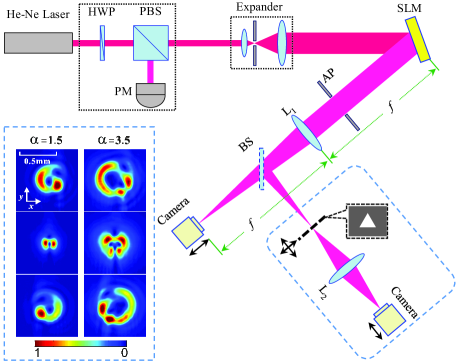
Figure 1: (Color) Experimental setup for measuring intensity distributions of FVBs near the focal plane of a 2-$f$ lens system. When a beam splitter (BS) is inserted after the lens L₁, the reflected light is used for verifying their topological charges by using a triangle aperture placed on a two-axis translation stage. Left insert figure is experimental intensity measurement of FVBs with $\alpha=1.5$ and 3.5, respectively, locating at 40 mm before (top), at (middle), and at 40 mm after (bottom) the focal plane. The lens L₁ has a focal length $f=300$ mm. Other notations are: HWP, half-wave plate; PBS, polarized beam splitter; PM, power meter; SLM, spatial light modulator; AP, Aperture.

Meanwhile, in order to obtain the spatial-frequency variances $(\Delta\theta_{q})^{2}$ at far-field zone, here a 2-$f$ focusing system with a focal length $f$ (as shown in Fig. 1) is employed and enables us to measure the far-field intensity distribution at its focal plane. The ray transfer matrix of such a 2-$f$ focusing system is given by $\left(\begin{smallmatrix}A&B\\ C&D\end{smallmatrix}\right)=\left(\begin{smallmatrix}0&f\\ -1/f&0\end{smallmatrix}\right)$ at the focal plane, therefore the output field at the focal plane is expressed by $E_{\text{o}}(x,y,f)=\frac{\exp(2ikf)}{i\lambda f}\iint E_{\text{i}}(u,v,0)\exp\left[-\frac{ik}{f}(xu+yv)\right]dudv$. This expression is very similar to the Fraunhofer diffraction equation of the far field. According to the definition of spatial-frequency variables, $\theta_{q}=q/(\lambda f)$, the field profile at focal plane changes into: $E_{\text{o}}(\theta_{x},\theta_{y},f)=\frac{\exp(2ikf)}{i\lambda f}\iint E_{\text{i}}(u,v,0)\exp\left[-i2\pi(\theta_{x}u+\theta_{y}v)\right]dudv$. Once one obtains the distribution $\left|E_{\text{o}}(\theta_{x},\theta_{y},f)\right|^{2}$ from the camera which is located at the focal plane (see Fig. 1), $(\Delta\theta_{q})^{2}$ can be evaluated through the following second-order moment Siegman1990

$$\left(\Delta\theta_{q}\right)^{2}=\frac{\iint(\theta_{q}-\bar{\theta}_{q})^{2}\left|E_{\text{o}}(\theta_{x},\theta_{y},f)\right|^{2}d\theta_{x}d\theta_{y}}{\iint\left|E_{\text{o}}(\theta_{x},\theta_{y},f)\right|^{2}d\theta_{x}d\theta_{y}}\text{,}$$ (10)

where $\bar{\theta}_{q}=\frac{\iint\theta_{q}\left|E_{\text{o}}(\theta_{x},\theta_{y},f)\right|^{2}d\theta_{x}d\theta_{y}}{\iint\left|E_{\text{o}}(\theta_{x},\theta_{y},f)\right|^{2}d\theta_{x}d\theta_{y}}$ are the average values of transverse spatial frequencies. In principle the values $(\Delta\theta_{q})^{2}$ are not related with the focal length $f$. However, in order to obtain the good quality of intensity distribution on the camera, we use a lens with a long focal length ($f=1000$ mm and $300$ mm) in the experiment.

Another quantity to describe vortex beams is the vortex strength, which is a unique quantity describing the phase structures associated with orbital angular momentum of FVBs. Since the evolution of FVBs in free space is very complex and there are infinite pairs of positive and negative vortices Berry2004 ; Leach2004 ; Lee2004 , we also consider the vortex strength at the focal plane of a 2-$f$ focusing system. The total vortex strength in cylindrical coordinates is written as Berry2004 ; Jesus2012

$$S_{\alpha} =\underset{\rho\rightarrow\infty}{\lim}\frac{1}{2\pi}\int_{0}^{2\pi}d\varphi\arg E_{\text{o,}\alpha}(\rho,\varphi,f)$$

$$=\underset{\rho\rightarrow\infty}{\lim}\frac{1}{2\pi}\int_{0}^{2\pi}d\varphi\text{Re}[iE_{\text{o,}\alpha}^{-1}(\rho,\varphi,f)\partial E_{\text{o,}\alpha}(\rho,\varphi,f)/\partial\varphi].$$ (11)

Here we emphasize that, at the focal plane of a 2-$f$ focusing system, such FVBs have a finite number of vortices, thus it is more convenient to investigate the vortex strength of beams at this plane. In order to verify the vortex strength, we use two experimental methods to identify all vortices contained in FVBs at the focal plane.

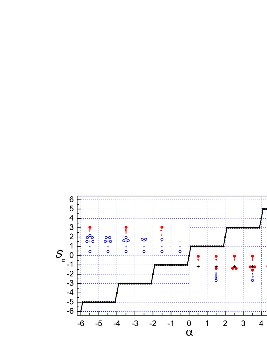
Figure 2: (Color) Numerical results of the vortex strength of FVBs at focal plane as a function of topological charge $\alpha$ with steps of 0.1. The inset figures are the schematic diagrams of vortex dynamics for FVBs at focal plane as $\alpha$ increases within each interval between any two integers, where red-solid and blue-open circles, respectively, denote the vortices with +1 and -1 charge. The arrows indicate the movement directions of new vortices, and the cross symbol is the geometric center on the focal plane.

III Experimental Results and Discussions

Our main experimental setup is shown in Fig. 1. A SLM (Holoeye PLUTO-2-VIS-056) is used for reconstruct a FVB, and it is illuminated by a He-Ne linear-polarized fundamental-mode laser beam with wavelength 632.8 nm. Here the SLM is applied by grayscale sinusoidal-like holograms, which are generated first by interfering the wanted first order diffracting beam hosting the fractional phase azimuthal variation with a plane wave mathematically, thus the first-order diffraction field in the output field from the SLM is a FVB. Of course, this SLM can also directly load the patterns of fractional spiral phase structures, and the output field directly becomes a FVB. The half-wave plate (HWP) and the beam polarized splitter (PBS) are assembly used to control the intensity of the incident beam. The output beam from the PBS is horizontal polarization (along $x$ direction). The expander consists of a pair of lenses and an aperture, which roughly expands the beam waist to $w_{0}\approx 1$ mm. The SLM is placed within the collimated distance of the beam after the expander. After modulating by the SLM, the light fields become the wanted vortex beams with various topological charges, which via a 2-$f$ lens system are carefully recorded by a camera. In our experiment, in order to reduce the measure error, we chose two different lenses (L₁) with $f=300$ mm and $f=1000$ mm to repeatedly measure the intensity distributions near or at their focal planes, and meanwhile the 2-$f$ lens system should be precisely adjusted by keeping both the distances from the SLM to L₁ and from L₁ to the camera equal to $f$. The camera sensor (Sony IMX183(M)) has a $13.06$ mm $\times 8.76$ mm exposure area with each pixel size of $2.4$ $\mu$m $\times 2.4$ $\mu$m and real-time 12-bit data depth.

In the inset of Fig. 1, it shows the intensity distributions of FVBs with $\alpha=1.5$ and $3.5$, respectively, locating before, at, and after the L₁’s focal plane. When the position of the camera is at the focal plane, the intensity profile is exactly symmetric about $y$ axis and all vortices (or called as singularities) in light fields are aligned (or symmetric) with $y$ axis; while when it is away from the focal plane, the intensity profile is not symmetric any more and noncentral vortices rotate around the geometric center of $x$-$y$ plane. This property enables us to accurately measure the intensity distributions at focal plane of such a 2-$f$ lens system. According to the formula in the previous section, we can acquire the information of both $|E_{\text{o}}(x,y,f)|^{2}$ and $|E_{\text{o}}(\theta_{x},\theta_{y},f)|^{2}$. Note that we should consider both the size of the pixels on the camera and the value of $f$ to get $|E_{\text{o}}(\theta_{x},\theta_{y},f)|^{2}$. Meanwhile, we also record the input intensity distributions $|E_{\text{i}}(u,v,0)|^{2}$ at the position of the SLM, and these input intensities are also repeatedly measured for better determining practical values of $w_{x}$ and $w_{y}$. From $|E_{\text{o}}(\theta_{x},\theta_{y},f)|^{2}$, one can know the values of $(\Delta\theta_{q})^{2}$.

Before we discuss our experimental results, in Fig. 2, let us first see the numerical result on total vortex strength $S_{\alpha}$ of such FVBs as a function of topological charge $\alpha$. Different from the previous results Berry2004 ; Jesus2012 , here we observe the jumps in $S_{\alpha}$ only when $\alpha$ is around any even number (i.e., $\alpha=0,\pm 2,\pm 4,\pm 6,\cdots$). Actually there are two continuous jumps around each even integer number: the first jump is that $S_{\alpha}$ increases 1 when $\alpha$ approaches to any even integer, and $S_{\alpha}$ exactly equals to that even integer when $\alpha$ is an even integer, and the second jump is that $S_{\alpha}$ continues to increase 1 when $\alpha$ is slightly larger than any even number. However, in Ref. Berry2004 , the jumps in $S_{\alpha}$ happen at every half-integer value of $\alpha$, and $S_{\alpha}$ only increases 1 at each jump for indicating a birth of a vortex; and in Ref. Jesus2012 , each jump leads to a unit change in $S_{\alpha}$ only at $\alpha=n+\varepsilon$, where $n$ is an integer and $\varepsilon$ is a small fraction. From Fig. 2, it can be concluded that

$$S_{\alpha}=\left\{\begin{array}[c]{c}m,\text{ \ \ \ \ \ \ \ \ \ for }\alpha=m\text{\ \ }\\ 2m-1,\text{ for }2(m-1)<\alpha<2m\end{array}\right.$$ (12)

where $$m S_{\alpha}$$ is integer. Here we would like to point out that the jumps in here do not completely indicate the birth of a vortex. These features will be explained next by phase structures and the dynamics of vortices at focal plane.

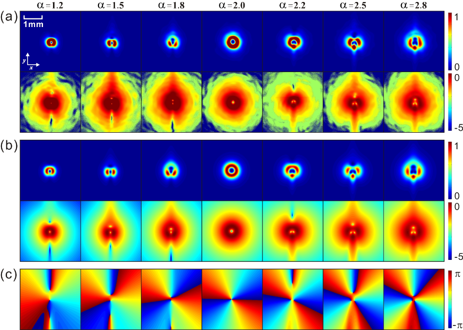
Figure 3: (Color) (a) Experimental and (b) numerical results of typical intensity distributions for FVBs with different values $\alpha$ from 1.2 (left) to 2.8 (right). The corresponding numerical phase structures are plotted in (c). In (a) and (b), the first and second rows are, respectively, in normal and logarithmic scales. Here we use the lens L₁ with $f=1000$ mm.

Figure 3 (a) experimentally shows typical intensity distributions of FVBs with different values $\alpha$ at focal plane. In order to prominently display the singularities in low-intensity regions of light fields, the camera measuring intensities works at overexposed mode for the second row of Fig. 3(a). It is seen that there are three deep-dark regions for $\alpha=1.2$, $1.5$, and $1.8$. The position of the near-center dark region (this vortex with $+1$ charge) only suffers little change due to the movement of a pair of top and bottom vortices. From $\alpha=1.2$ to $1.5$ in Fig. 3(a), it is observed that both the top and bottom vortices, with $+1$ and $-1$ charges, respectively, approach to the center vortex, but the top vortex with $+1$ charge moves faster than the bottom one; while from $\alpha=1.5$ to $1.8$, the top vortex continues to close the near-center vortex but the bottom vortex quickly leaves away from the near-center vortex, also see the schematic dynamics of vortices in the inset of Fig. 2. When $\alpha=2$, the top vortex completely merges with the center vortex, and the bottom vortex moves to infinity (or say, it disappears). Thus there is a jump in $S_{\alpha}$ in Fig. 2 when $\alpha$ closes to 2, because a vortex with $-1$ charge disappears.

For $\alpha=2.2$ to $2.8$ in Fig. 3, one can observe that there are still three-dark regions (singularities): two vortices locate near the center and move very slightly, and other top vortex moves quickly from the outside to center. In fact, all these three vortices have the same $+1$ charge (experimentally verified below). Therefore, when $\alpha$ is slightly larger than 2, in principle a new vortex is born from outside infinity and it moves to the center as $\alpha$ closes to 3, also see the schematic dynamics in inset of Fig. 2. Experimental results in Fig. 3(a) are in good agreement with the corresponding numerical results in Fig. 3(b). For further demonstration on evolutions of these singularities (or vortices), the individual phase structures are also plotted in Fig. 3(c). Clearly, there occur a pair of positive and negative charge vortices for $\alpha\in(1,2)$, which leads $S_{\alpha}$ unchanged. Meanwhile a new +1 vortex is generated for $\alpha\in(2,3)$. From Fig. 2 and Fig. 3, it is concluded that, when $2(m-1)<\alpha<2m-1$, $S_{\alpha}=2m-1$ and there is a new vortex moving from outside to center; when $2m-1<\alpha<2m$, $S_{\alpha}\$still equals to $2m-1$ but a pair of +1 and -1 charge vortices are generated. The layouts of all vortices for different FVBs at focal plane are also schematically plotted in Fig. 2. This explains the appearance of the two continuous jumps in $S_{\alpha}$ around each even number of $\alpha$.

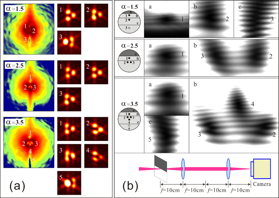
Figure 4: (Color) Experimental verification on the topological charge of each vortex in FVBs at the focal plane of a 2-$f$ lens system. (a) The vortex distributions in different FVBs (left), and the corresponding interference patterns (right) of individual vortices by the diffraction method of a tiny triangle aperture. (b) The interference patterns diffracted by the straight blade via a 4-$f$ lens system. Here the blade edge is moved from up to down, and is located at different positions a, b, or c [see the left sketch of each case in (b)], for detecting the fork-like interference patterns. The measurement system by the straight blade is also plotted in the bottom of (b). Each vortex and its interference patten in (a) and (b) are correspondingly marked with a number, and here the topological charge $\alpha=1.5,2.5,3.5.$

Then we ask ourselves that, are all these vortices in FVBs measurable? In order to solidly confirm our observations, we use two methods to confirm our findings in Fig. 2 and Fig. 3. In Fig. 4(a), it demonstrates the experimental verification of these vortices in FVBs by using a tiny equilateral triangle aperture (confirmed under an microscope). This kind of method for testing the vortex was proposed by Hickmann2010 and has been widely used to detect vortex due to its high efficiency and accuracy Jesus2012 ; Mourka2011 ; Anderson2012 . Here the triangle aperture is placed on a two-dimensional movable stage, locating at the L₁’s focal plane via the reflection of the BS. This measurement optical system is shown in Fig. 1, and another 2-$f$ system of the lens L₂ is used to collect interference pattern at its focal plane. From Fig. 4(a), for $\alpha=1.5$, three vortices in intensity are detected and verified. It is seen that the 1st and 2nd interference patterns for both the top and near-center vortices are the same and indicate the vortices with +1 charge, but the 3rd pattern for the bottom vortex is rotated by $\pi$ and it indicates this vortex with $-1$ charge. For $\alpha=2.5$, it is not difficult to observe each interference pattern for each vortex and all these patterns indicate the vortices having the same sign with +1 charge. For $\alpha=3.5$, there are similar patterns for the top and three near-center vortices with labels 1 to 4, indicating the same sign with +1 charge, but the last pattern for the bottom vortex with label 5 is also rotated by $\pi$ and it tells us that it is a negative vortex with -1 charge. It should be noted that one has to increase the input power of laser in order to measure the bottom vortices in cases of $\alpha=1.5$ and $3.5$ because their intensities are usually very weak.

Another verification measurement system is shown in the bottom of Fig. 4(b). It consists of two lenses forming a 4-$f$ optical system, which can inversely image the pattern located at its input plane. However, due to the diffraction from the edge of the straight blade, when the blade edge approaches a vortex contained in light fields, one can observe a fork-like interference pattern at the image plane. Via zooming in interference patterns, it is seen that there are fork-like interference fringes, which are formed from the interference between an optical vortex contained in light fields and an edge diffraction wave by the blade edge. The open direction of the fork indicates the sign of a vortex. For example, when $\alpha=1.5$, one can see that the 1st and 2nd fork interference fringes are similar and indicate the vortices with +1 charge at the fork centers, and the 3rd fork fringes have opposite directions, which denote a vortex with -1 charge existing at its fork center. Similarly, one can use this method to determine all vortices for the cases of $\alpha=2.5$ and $3.5$ by moving the blade edge. In a word, this method again confirms that a pair of positive and negative vortices exist for $\alpha=1.5$ and $3.5$, and all vortices have the same sign for $\alpha=2.5$. By this method, one can verify other situations for different $\alpha$. Therefore we conclude that total $S_{\alpha}$ for FVBs follows Fig. 2, which is different from Refs. Berry2004 ; Jesus2012 .

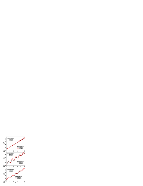
Figure 5: (Color) Experimental results (black and red dots), and matched numerical results (black and red dashed lines) of the BPF values in (a) $x$-direction, (b) $y$-direction, and (c) total BPF values of FVBs as functions of $\alpha$ with steps of 0.1. The error bars are obtained from multiple measurements and the focal length of the lens L₁ is chosen to be $f=300$ mm and $f=1000$ mm for two groups of multiple measurements.

As we presented in the section II, the distributions of light fields at focal plane represent the behavior of light at far-field regions. In Refs. Leach2004 , one already knew that there are rotation processes of vortex during the propagations of FVBs in free space, and both birth and annihilation phenomena of vortices may happen as $\alpha$ increases. From above discussions, when $\alpha$ increases, the vortices in FVBs show different traces moving on focal plane. Hence, it is very meaningful to evaluate the BPF of such FVBs, which is never investigated before. Figure 5 shows the measured results of BPF values as a function of topological charge $\alpha$. It is observed in Fig. 5(a) and 5(b) that as $\alpha$ increases, the BPF $M_{x}^{2}$ in $x$-direction almost increases linearly, while $M_{y}^{2}$ in $y$-direction increases with oscillations. Different behaviors of $M_{x}^{2}$ and $M_{y}^{2}$ can be understood by intensity distributions at focal plane from Fig. 3. The intensity distributions for such beams are always symmetric in $x$ direction at focal plane or at far-field region of free space, and the effective diverging angle (also corresponding to the effective spread of spatial frequency) almost increases linearly too as $\alpha$ increases. However, in $y$ direction, a vortex or a pair of vortices at focal plane can be born periodically with the increase of $\alpha$, and their movements (see the sketch in Fig. 2) along $y$ direction lead to the oscillations in $M_{y}^{2}$. The numerical curves are obtained by substituting Eq. (7) into Eq. (10) and using Eqs. (8a) and (8b), and the numerical integration range in Eq. (10) should be matched with experimental data, because the numerator integration of Eq.(10) depends on its integrating range, and in practical sense, there are also the physical limitation of camera camera, which cannot record the intensity values lower than its threshold. It is seen that, when the numerical ranges are matched with the experimental data, the measured BPF values are in good agreement with the matched numerical results. When we average both $M_{x}^{2}$ and $M_{y}^{2}$ to define the total BPF $M_{T}^{2}=\frac{1}{2}(M_{x}^{2}+M_{y}^{2})$, then there are step-like jumps in $M_{T}^{2}$ as $\alpha$ increases, see Fig. 5(c). This curve has certain similarity to the practical changes of the effective OAM of such beams Alperin2016 ; Alperin2017 . For only integer values of $\alpha$, $M_{T}^{2}$ has similar property of linear increase, like those Laguerre-Gaussian beams as a function of integer azimuthal index $n$ Saghafi1998 ; Vega2007 .

IV Summary

In conclusion, we have studied the vortex strength and BPF of FVBs. Under paraxial approximation, we have derived the output filed for such FVBs passing through arbitrary linear ABCD optical system. From light fields at focal plane of a 2-$f$ lens system (similar to the far-field distribution), our results have demonstrated the vortex strength increases by unit continuously when topological charge is very close before and after an even number. Triangle aperture and straight blade, respectively, were employed to experimentally detect the vortices of FVBs at focal plane and to confirm each vortex charge, and thus the change of vortex strength for FVBs is confirmed. The experimental results, demonstrating the movement of all vortices at focal plane, are in good agreement with the numerical results, and the dynamics of all vortices at focal plane are different in two intervals of topological charges. The BPF value has been used to describe the characteristics of propagation behavior of FVBs. Experimental results show that as the topological charge increases, the value of BPF increases linearly in $x$-component while the obvious oscillations exist in the BPF value in $y$-component. Moreover, there are step-like jumps in the total BPF values as the topological charge increases, which have a similar behavior to the OAM of FVBs as the topological charge increases. Our findings will bring distinct perspectives to the research of vortex strength at focal plane and the BPF value for both FVBs and other complex structured light fields.

- (1) L. Allen, M. W. Beijersbergen, R. J. C. Spreeuw, and J. P. Woerdman, Orbital angular momentum of light and the transformation of Laguerre-Gaussian laser modes, Phy. Rev. A 45, 8185 (1992).
- (2) M. V. Berry, Optical vortices evolving from helicoidal integer and fractional phase steps, J. Opt. A: Pure Appl. 6, 259 (2004).
- (3) J. Leach, E. Yao, and M. J. Padgett, Observation of the vortex structure of a non-integer vortex beam, New J. Phys. 6, 71 (2004).
- (4) S. N. Alperin, and M. E. Siemens, Angular momentum of topologically structured darkness, Phy. Rev. Lett. 119, 203902 (2017).
- (5) G. Tkachenko, M. Z. Chen, K. Dholakia, and M. Mazilu, Is it possible to create a perfect fractional vortex beam?, Optica 4, 330 (2017).
- (6) S. H. Tao, X. C. Yuan, J. Lin, X. Peng, and H. B. Niu, Fractional optical vortex beam induced rotation of particles, Opt. Express 13, 7726 (2005).
- (7) G. Gbur, Fractional vortex Hilbert’s hotel, Optica 3, 222 (2016).
- (8) Z. Y. Hong, J. Zhang, and B. W. Drinkwater, On the radiation force fields of fractional-order acoustic vortices, EPL 110, 14002 (2015).
- (9) Y. R. Jia, Q. Wei, D. J. Wu, Z. Xu, and X. J. Liu, Generation of fractional acoustic vortex with a discrete Archimedean spiral structure plate, Appl. Phys. Lett. 112, 173501 (2018).
- (10) P. Bandyopadhyay, B. Basu, and D. Chowdhury, Geometric phase and fractional orbital-angular-momentum states in electron vortex beams, Phy. Rev. A 95, 013821 (2017).
- (11) S. S. R. Oemrawsingh, A. Aiello, E. R. Eliel, G. Nienhuis, and J. P. Woerdman, How to observe high-dimensional two-photon entanglement with only two detectors, Phy. Rev. Lett. 92, 217901 (2004).
- (12) S. S. R. Oemrawsingh, X. Ma, D. Voigt, A. Aiello, E. R. Eliel, G. W. ’t Hooft, and J. P. Woerdman, Experimental demonstration of fractional orbital angular momentum entanglement of two photons, Phy. Rev. Lett. 95, 240501 (2005).
- (13) L. X. Chen, J. J. Lei, and J. Romero, Quantum digital spiral imaging, Light: Sci. Appl. 3, e153 (2014).
- (14) I. V. Basistiy, M. S. Soskin, and M. V. Vasnetsov, Optical wavefront dislocations and their properties, Opt. Commun. 119, 604 (1995).
- (15) I. V. Basistiy, V. A. Pas’ko, V. V. Slyusar, M. S. Soskin, and M. V. Vasnetsov, Synthesis and analysis of optical vortices with fractional topological charges, J. Opt. 6, S166 (2004).
- (16) S. N. Alperin, R. D. Niederriter, J. T. Gopinath, and M. E. Siemens, Quantitative measurement of the orbital angular momentum of light with a single, stationary lens, Opt. Lett. 41, 5019 (2016).
- (17) W. M. Lee, X. C. Yuan, and K. Dholakia, Experimental observation of optical vortex evolution in a Gaussian beam with an embedded fractional phase step, Opt. Commun. 239, 129 (2004).
- (18) Y. Q. Fang, Q. H. Lu, X. L. Wang, W. H. Zhang, and L. X. Chen, Fractional-topological-charge-induced vortex birth and splitting of light fields on the submicron scale, Phy. Rev. A 95, 023821 (2017).
- (19) A. J. Jesus-Silva, E. J. S. Fonseca, and J. M. Hickmann, Study of the birth of a vortex at Fraunhofer zone, Opt. Lett. 37, 4552 (2012).
- (20) A. E. Siegman, New developments in laser resonators, Proc. SPIE 1224, 2 (1990).
- (21) R. Borghi and M. Santarsiero, factor of Bessel-Gauss beams, Opt. Lett. 22, 262 (1997).
- (22) M. A. Porras, R. Borghi, and M. Santarsiero, Relationship between elegant Laguerre-Gauss and Bessel-Gauss beams, J. Opt. Soc. Am. A 18, 177 (2001).
- (23) S. Saghafi, and C. J. R. Sheppard, The beam propagation factor for higher order Gaussian beams, Opt. commun. 153, 207 (1998).
- (24) J. C. Gutiérrez-Vega, Fractionalization of optical beams: II. Elegant Laguerre-Gaussian modes, Opt. Express 15, 6300 (2007).
- (25) S. Ramee and R. Simon, Effect of holes and vortices on beam quality, J. Opt. Soc. Am. A 17, 84 (2000).
- (26) S. A. Collins, Lens-system diffraction integral written in terms of matrix optics, J. Opt. Soc. Am. 60, 1168 (1970).
- (27) S. Wang, and D. Zhao, Matrix Optics, (Springer, Berlin, 2000).
- (28) J. M. Hickmann, E. J. S. Fonseca, W. C. Soares, and S. Chávez-Cerda, Unveiling a truncated optical lattice associated with a triangular aperture using light’s orbital angular momentum, Phys. Rev. Lett. 105, 053904 (2010).
- (29) A. Mourka, J. Baumgartl, C. Shanor, K. Dholakia, and E. M. Wright, Visualization of the birth of an optical vortex using diffraction from a triangular aperture, Opt. Express 19, 5760 (2011).
- (30) M. E. Anderson, H. Bigman, L. E. E. de Araujo, and J. L. Chaloupka, Measuring the topological charge of ultrabroadband, optical-vortex beams with a triangular aperture, J. Opt. Soc. Am. B 29, 1968 (2012).