Quantum spins and random loops
on the complete graph

Abstract.

We present a systematic analysis of quantum Heisenberg-, xy- and interchange models on the complete graph. These models exhibit phase transitions accompanied by spontaneous symmetry breaking, which we study by calculating the generating function of expectations of powers of the averaged spin density. Various critical exponents are determined. Certain objects of the associated loop models are shown to have properties of Poisson–Dirichlet distributions.

1. Introduction

We study phase transitions accompanied by spontaneous symmetry breaking in quantum spin systems with two-body interactions on the complete graph. Among models analyzed in this paper are the quantum Heisenberg ferromagnet, the quantum xy-model, and the “quantum interchange model” where interactions are expressed in terms of the “transposition operator”. For these models, we investigate the structure of the space, $\Psi_{\beta}$, of extremal Gibbs states at inverse temperature $\beta=(kT)^{-1}$, for different values of $\beta$. Following a suggestion of Thomas Spencer, we analyze the generating function, $\Phi_{\beta}(h)$, of correlations of the averaged spin density in the symmetric Gibbs state at inverse temperature $\beta$, which depends on a symmetry-breaking external magnetic field, $h$. The function $\Phi_{\beta}(h)$ can be viewed as a Laplace transform of the measure d$\mu$ on $\Psi_{\beta}$ whose barycenter is the symmetric Gibbs state at inverse temperature $\beta$. Its usefulness lies in the fact that it sheds light on the structure of the space of extremal Gibbs states. We calculate $\Phi_{\beta}(h)$ explicitly for a class of (mean-field) spin models defined on the complete graph, for all values of $\beta>0$. It is expected that the dependence of $\Phi_{\beta}(h)$ on the external magnetic field $h$ is universal, in the sense that it is equal to the one calculated for the corresponding models defined on the lattice ${\mathbb{Z}}^{d}$, provided the dimension $d$ satisfies $d\geq 3$. Moreover, the structure of $\Psi_{\beta}$ is expected to be independent of $d$, for $d\geq 3$, and identical to the one in the models on the complete graph. Rigorous proofs, however, still elude us.

The quantum spin systems studied in this paper happen to admit random loop representations, and the functions $\Phi_{\beta}(h)$ correspond to characteristic functions of the lengths of random loops. It turns out that these characteristic functions are equal to those of the Poisson–Dirichlet distribution of random partitions. This is a strong indication that the joint distribution of the lengths of the random loops is indeed the Poisson–Dirichlet distribution.

Next, we briefly review the general theory of extremal-states decompositions. (For more complete information we refer the reader to the 1970 Les Houches lectures of the late O. E. Lanford III [19], and the books of R. B. Israel [15] and B. Simon [27].) The set, $\mathcal{G}_{\beta}$, of infinite-volume Gibbs states at inverse temperature $\beta$ forms a Choquet simplex, i.e., a compact convex subset of a normed space with the property that every point can be expressed uniquely as a convex combination of extreme points, (i.e., as the barycenter of a probability measure supported on extreme points). As above, let $\Psi_{\beta}\subset\mathcal{G}_{\beta}$ denote the space of extremal Gibbs states at inverse temperature $\beta$. Henceforth we denote an extremal Gibbs state by $\langle\cdot\rangle_{\psi}$, with $\psi\in\Psi_{\beta}$. Since $\mathcal{G}_{\beta}$ is a Choquet simplex, an arbitrary state $\langle\cdot\rangle\in{\mathcal{G}}_{\beta}$ determines a unique probability measure d$\mu$ on $\Psi_{\beta}$ such that

$$\langle\cdot\rangle=\int_{\Psi_{\beta}}\langle\cdot\rangle_{\psi}\,{\rm d}\mu(\psi).$$ (1.1)

At small values of $\beta$, i.e., high temperatures, the set ${\mathcal{G}}_{\beta}$ of Gibbs states at inverse temperature $\beta$ contains a single element, and the above decomposition is trivial. The situation tends to be more interesting at low temperatures: the set ${\mathcal{G}}_{\beta}$ may then contain many states, in which case one would like to characterise the set $\Psi_{\beta}$ of extreme points of ${\mathcal{G}}_{\beta}$.

In the models studied in this paper, the Hamiltonian is invariant under a continuous group, $G$, of symmetries, and the set ${\mathcal{G}}_{\beta}$ of Gibbs states at inverse temperature $\beta$ carries an action of the group $G$. At low temperatures, this action tends to be non-trivial; i.e., there are plenty of Gibbs states that are not invariant under the action of $G$ on $\mathcal{G}_{\beta}$. This phenomenon is referred to as “spontaneous symmetry breaking”. For the models studied in this paper, the space $\Psi_{\beta}$ of extremal Gibbs states is expected to consist of a single orbit of an extremal state $\langle\cdot\rangle_{\psi_{0}},\psi_{0}\in\Psi_{\beta},$ under the action of $G$ (this is clearly a special case of the general situation). Then $\Psi_{\beta}\simeq G/H$, where $H$ is the largest subgroup of $G$ leaving $\langle\cdot\rangle_{\psi_{0}}$ invariant, and the symmetric (i.e., $G$-invariant) state in ${\mathcal{G}}_{\beta}$ can be obtained by averaging over the orbit of the state $\langle\cdot\rangle_{\psi_{0}}$ under the action of the group $G$ using the (uniform) Haar measure on $G$.

As announced above, we will follow a suggestion of T. Spencer and attempt to characterise the set $\Psi_{\beta}$ by considering a Laplace transform $\Phi_{\beta}(h)$ of the measure on $\Psi_{\beta}$ whose barycenter is the symmetric state. We describe the general ideas of our analysis for models of quantum spin systems defined on a lattice $\mathbb{Z}^{d},d\geq 3$; afterwards we will rigorously study similar models defined on the complete graph. At each site $i\in\mathbb{Z}^{d}$, there are $N$ operators $\vec{S}_{i}=(S^{(1)},\dots,S^{(N)})$ describing a “quantum spin” located at the site $i$. We assume that the symmetry group $G$ is represented on the algebra of spin observables generated by the operators $\{\vec{S}_{i}\mid i\in\mathbb{Z}^{d}\}$ by ^∗-automorphisms, $\alpha_{g},g\in G$, with the property that there exist $N\times N$- matrices $R(g),g\in G,$ acting transitively on the unit sphere $S^{N-1}\subset\mathbb{R}^{N}$ such that

$$\alpha_{g}(\vec{S}\cdot\vec{n})=\vec{S}\cdot R(g)\vec{n},\quad\forall\vec{n}\in\mathbb{R}^{N}.$$ (1.2)

We assume that the states $\langle\cdot\rangle_{\psi},\,\psi\in\Psi_{\beta},$ are invariant under lattice translations. Denoting by $\langle\cdot\rangle_{\Lambda,\beta}$ the symmetric Gibbs state in a finite domain $\Lambda\subset{\mathbb{Z}}^{d}$, and by $\Lambda\Uparrow{\mathbb{Z}}^{d}$ the standard infinite-volume limit (in the sense of van Hove), we consider the generating function

$$\begin{split}\lim_{\Lambda\Uparrow{\mathbb{Z}}^{d}}\big{\langle}\,{\rm e}^{\frac{h}{|\Lambda|}\sum_{i\in\Lambda}S_{i}^{(1)}}\,\big{\rangle}_{\Lambda,\beta}&\overset{(?)}{=}\lim_{\Lambda\Uparrow{\mathbb{Z}}^{d}}\lim_{\Lambda^{\prime}\Uparrow{\mathbb{Z}}^{d}}\big{\langle}\,{\rm e}^{\frac{h}{|\Lambda|}\sum_{i\in\Lambda}S_{i}^{(1)}}\,\big{\rangle}_{\Lambda^{\prime},\beta}\\ &=\lim_{\Lambda\Uparrow{\mathbb{Z}}^{d}}\int_{\Psi_{\beta}}\big{\langle}\,{\rm e}^{\frac{h}{|\Lambda|}\sum_{i\in\Lambda}S_{i}^{(1)}}\,\big{\rangle}_{\psi}\,{\rm d}\mu(\psi)\\ &=\int_{\Psi_{\beta}}\,{\rm e}^{h\langle S_{0}^{(1)}\rangle_{\psi}}\,{\rm d}\mu(\psi).\end{split}$$ (1.3)

Here, $S_{0}^{(1)}$ is the spin operator $S^{(1)}$ acting at the site $0$. The first identity is expected to hold true in great generality; but it appears to be difficult to prove it in concrete models. The second identity holds under very general assumptions, but the exact structure of the space $\Psi_{\beta}$ and the properties of the measure d$\mu$ are only known for a restricted class of models, such as the Ising- and the classical xy-model. The third identity usually follows from cluster properties of connected correlations in extremal states.

Assuming that all equalities in (1.3) hold true, we define the (“spin-density”) Laplace transform of the measure d$\mu$ corresponding to the symmetric state by

$$\Phi_{\beta}(h)=\lim_{\Lambda\Uparrow{\mathbb{Z}}^{d}}\big{\langle}\,{\rm e}^{\frac{h}{|\Lambda|}\sum_{i\in\Lambda}S_{i}^{(1)}}\,\big{\rangle}_{\Lambda,\beta}=\int_{\Psi_{\beta}}\,{\rm e}^{h\langle S_{0}^{(1)}\rangle_{\psi}}\,{\rm d}\mu(\psi).$$ (1.4)

The action of $G$ on the space $\mathcal{G}_{\beta}$ of Gibbs states is given by

$$\langle\cdot\rangle\mapsto\langle\cdot\rangle^{g},\,\text{ where }\,\langle A\rangle^{g}:=\langle\alpha_{g^{-1}}(A)\rangle,$$

for an arbitrary spin observable $A$. As mentioned above, we will consider models for which it is expected that $\Psi_{\beta}$ is the orbit of a single extremal state, $\langle\cdot\rangle_{\psi_{0}}$; i.e., given $\psi\in\Psi_{\beta}$, there exists an element $g(\psi)\in G$ such that

$$\langle\cdot\rangle_{\psi}=\langle\cdot\rangle_{\psi_{0}}^{g(\psi)},$$ (1.5)

where $g(\psi)$ is unique modulo the stabilizer subgroup $H$ of $\langle\cdot\rangle_{\psi_{0}}$. Then we have that

$$\big{\langle}\vec{S}_{0}\big{\rangle}_{\psi}\cdot\vec{e}=\big{\langle}\alpha_{g(\psi)^{-1}}(\vec{S}_{0}\cdot\vec{e})\big{\rangle}_{\psi_{0}}=\big{\langle}\vec{S}_{0}\big{\rangle}_{\psi_{0}}\cdot R(g(\psi)^{-1})\vec{e}.$$ (1.6)

Defining the magnetisation as $\vec{m}_{d}(\beta)=\langle\vec{S}_{0}\rangle_{\psi_{0}}$, we find that the spin-density Laplace transform (1.4) is given by

$$\Phi_{\beta}(h)=\int_{\Psi_{\beta}}e^{h\,\vec{m}_{d}(\beta)\cdot R(g(\psi)^{-1})\vec{e}_{1}}\,{\rm d}\mu(\psi),$$ (1.7)

where $\vec{e}_{1}$ is the unit vector in the $1$-direction in $\mathbb{R}^{N}$; (actually, $\vec{e}_{1}$ can be replaced by an arbitrary unit vector in $\mathbb{R}^{N}$).

In this paper we study a variety of quantum spin systems for which we will calculate the function $\Phi_{\beta}(h)$ in two different ways:

1. For an explicit class of models defined on the complete graph, we are able to calculate the function $\Phi_{\beta}(h)$ explicitly and rigorously.

2. On the basis of some assumptions on the structure of the set $\Psi_{\beta}$ of extremal Gibbs states and on the matrices $R(g),\,g\in G,$ that we will not justify rigorously, we are able to determine $\Phi_{\beta}(h)$ using (1.3).

We then observe that the two calculations yield identical results, representing support for the assumptions underlying calculation (2).

Organization of the paper

In Section 2 we provide precise statements of our results and verify that they are consistent with the heuristics captured in Eq. (1.3). In Section 3 we describe (known) representations of the spin systems considered in this paper in terms of random loops; we then discuss probabilistic interpretations of our results and relate them to the Poisson–Dirichlet distribution. In Sections 4 through 7, we present proofs of our results. Some auxiliary calculations and arguments are collected in four appendices.

2. Setting and results

In this section we describe the precise setting underlying the analysis presented in this paper. Rigorous calculations will be limited to quantum models on the complete graph.

Let $n\in{\mathbb{N}}$ be the number of sites, and let $S\in\frac{1}{2}{\mathbb{N}}$ be the spin quantum number. The state space of a model of quantum spins of spin $S$ located at the sites $\{1,\dots,n\}$ is the Hilbert space ${\mathcal{H}}_{n}=({\mathbb{C}}^{2S+1})^{\otimes n}$. The usual spin operators acting on $\mathcal{H}_{n}$ are denoted by $\vec{S}_{j}=(S_{j}^{(1)},S_{j}^{(2)},S_{j}^{(3)})$, with $1\leq j\leq n$. They obey the commutation relations

$$[S_{j}^{(1)},S_{k}^{(2)}]={\rm i}\,\delta_{jk}S_{j}^{(3)},$$ (2.1)

with further commutation relations obtained by cyclic permutations of 1,2,3; furthermore,

$$(S_{j}^{(1)})^{2}+(S_{j}^{(2)})^{2}+(S_{j}^{(3)})^{2}=S(S+1){\bf{1}}.$$ (2.2)

The Hamiltonian, $H_{n,\Delta}^{\rm Heis}$, of the quantum Heisenberg model is given by

$$H_{n,\Delta}^{\rm Heis}=-\frac{2}{n}\sum_{1\leq i<j\leq n}\bigl{(}S_{i}^{(1)}S_{j}^{(1)}+S_{i}^{(2)}S_{j}^{(2)}+\Delta S_{i}^{(3)}S_{j}^{(3)}\bigr{)}\,,\qquad\Delta\in[-1,1].$$ (2.3)

The value $\Delta=0$ corresponds to the xy-model, and $\Delta=1$ corresponds to the usual Heisenberg ferromagnet. By $\langle\cdot\rangle^{\rm Heis}_{n,\beta,\Delta}$ we denote the corresponding Gibbs state

$$\langle\cdot\rangle^{\rm Heis}_{n,\beta,\Delta}=\frac{1}{{\operatorname{Tr\,}}[\,{\rm e}^{-\beta H_{n,\Delta}^{\rm Heis}}\,]}{\operatorname{Tr\,}}[\cdot\,{\rm e}^{-\beta H_{n,\Delta}^{\rm Heis}}\,].$$ (2.4)

The Hamiltonian of the quantum interchange model is chosen to be

$$H_{n}^{\rm int}=-\frac{1}{n}\sum_{1\leq i<j\leq n}T_{i,j}\,,$$ (2.5)

where the operators $T_{i,j}$ are the transposition operators defined by

$$T_{i,j}\,|\varphi_{1}\rangle\dots\otimes|\varphi_{i}\rangle\dots\otimes|\varphi_{j}\rangle\dots\otimes|\varphi_{n}\rangle=|\varphi_{1}\rangle\dots\otimes|\varphi_{j}\rangle\dots\otimes|\varphi_{i}\rangle\dots\otimes|\varphi_{n}\rangle\,,$$ (2.6)

where the vectors $|\varphi_{i}\rangle$ belong to the space $\mathbb{C}^{2S+1}$, for all $i=1,2,\dots,n$. The transposition operators are invariant under unitary transformations of $\mathbb{C}^{2S+1}$ and can be expressed using spin operators; see [22] or [9, Appendix A] for more details. Recall that the eigenvalues of $(\vec{S}_{i}+\vec{S}_{j})^{2}$ are given by $\lambda(\lambda+1)$, with $\lambda=0,1,\dots,2S$; hence the eigenvalues of $2\vec{S}_{i}\cdot\vec{S}_{j}$ are given by $\lambda(\lambda+1)-2S(S+1)$. Denoting by $P_{\lambda}$ the corresponding spectral projections we find that

$$T_{i,j}=\sum_{\lambda=0}^{2S}(-1)^{\lambda+1}P_{\lambda}=\sum_{\lambda=0}^{2S}(-1)^{2S-\lambda}\prod_{\lambda^{\prime}\neq\lambda}\frac{2\vec{S}_{i}\cdot\vec{S}_{j}-\lambda^{\prime}(\lambda^{\prime}+1)+2S(S+1)}{\lambda(\lambda+1)-\lambda^{\prime}(\lambda^{\prime}+1)}.$$ (2.7)

It is apparent that $T_{i,j}$ is a linear combination of $(\vec{S}_{i}\cdot\vec{S}_{j})^{k}$, with $k=0,1,\dots,2S$. One checks that

$$T_{i,j}=\begin{cases}2\vec{S}_{i}\cdot\vec{S}_{j}+\tfrac{1}{2}{\bf 1}&\text{if }S=\tfrac{1}{2},\\ (\vec{S}_{i}\cdot\vec{S}_{j})^{2}+\vec{S}_{i}\cdot\vec{S}_{j}-{\bf 1}&\text{if }S=1.\end{cases}$$ (2.8)

If $S=\frac{1}{2}$ the quantum interchange model is equivalent to the Heisenberg ferromagnet, but this is not the case for other values of the spin quantum number $S$. (The expressions for $T_{i,j}$, with $S\geq\frac{3}{2}$, look unappealing.) The Gibbs state of the quantum interchange model is given by

$$\langle\cdot\rangle^{\rm int}_{n,\beta}=\frac{1}{{\operatorname{Tr\,}}[\,{\rm e}^{-\beta H_{n}^{\rm int}}\,]}{\operatorname{Tr\,}}[\cdot\,{\rm e}^{-\beta H_{n}^{\rm int}}\,]\,.$$ (2.9)

2.1. Heisenberg and xy-models

First we consider the Heisenberg model with $\Delta=1$ and arbitrary spin $S\in\frac{1}{2}{\mathbb{N}}$. In order to define the spontaneous magnetisation, we introduce a function $\eta:{\mathbb{R}}\to{\mathbb{R}}$ by setting

$$\eta(x)=\log\Big{(}\frac{\sinh(\frac{2S+1}{2}x)}{\sinh(\frac{1}{2}x)}\Big{)}.$$ (2.10)

(At $x=0$ we define $\eta(0)=\log(2S+1)$.) Its first and second derivatives are

$$\begin{split}&\eta^{\prime}(x)=\tfrac{2S+1}{2}\coth(\tfrac{2S+1}{2}x)-\tfrac{1}{2}\coth(\tfrac{1}{2}x),\\ &\eta^{\prime\prime}(x)=\tfrac{1}{4}\frac{\sinh^{2}(\frac{2S+1}{2}x)-(2S+1)^{2}\sinh^{2}(\frac{1}{2}x)}{\sinh^{2}(\frac{2S+1}{2}x)\,\sinh^{2}(\frac{1}{2}x)}.\end{split}$$ (2.11)

Note that this function is smooth at $x=0$, where $\eta^{\prime}(0)=0$. The second derivative is positive, and $\eta^{\prime}(\pm\infty)=\pm S$, so that the equation

$$\eta^{\prime}(x)=m,$$ (2.12)

has a unique solution for all $m\in(-S,S)$. We denote this solution by $x^{\star}(m)$. Lengthy calculations yield

$$x^{\star}(0)=0\,;\qquad\frac{{\rm d}x^{\star}}{{\rm d}m}(0)=\frac{3}{S^{2}+S}\,;\qquad\frac{{\rm d}^{2}x^{\star}}{{\rm d}m^{2}}(0)=0\,.$$ (2.13)

Next, we define a function $g_{\beta}$ by

$$g_{\beta}(m):=\eta\bigl{(}x^{\star}(m)\bigr{)}-mx^{\star}(m)+\beta m^{2},\qquad m\in[0,S).$$ (2.14)

One finds that

$$g_{\beta}(0)=\log(2S+1);\qquad g_{\beta}^{\prime}(0)=0;\quad\text{ and }\quad g_{\beta}^{\prime\prime}(0)=2\beta-\frac{3}{S^{2}+S}.$$ (2.15)

Let $m^{\star}(\beta)\in[0,S)$ be the maximiser of $g_{\beta}$. From (2.15) we infer that $m^{\star}(\beta)>0$ if and only if $\beta$ is greater than the critical inverse temperature $\beta_{c}$ given by

$$\beta_{\rm c}=\frac{3/2}{S^{2}+S}.$$ (2.16)

It may be useful to note that, for $S=\frac{1}{2}$, the above definitions simplify considerably:

$$g_{\beta}(m)=\beta m^{2}-(\tfrac{1}{2}-m)\log(\tfrac{1}{2}-m)-(\tfrac{1}{2}+m)\log(\tfrac{1}{2}+m).$$ (2.17)

One easily checks that $g_{\beta}^{\prime}(0)=0$, $g_{\beta}^{\prime\prime\prime}(m)<0$ for all $m\in(0,\frac{1}{2})$, and that $g_{\beta}^{\prime\prime}(0)=2\beta-4$ is positive if and only if $\beta>2$. It follows that the unique maximiser $m^{\star}(\beta)$ is positive if and only if $\beta>2$; see Fig. 1. For the symmetric spin-$\tfrac{1}{2}$ Heisenberg model ($S=\tfrac{1}{2}$ and $\Delta=1$), the magnetisation $m^{\star}(\beta)$ was first identified by Tóth [30] and Penrose [24]. (See also the recent paper [4] by Alon and Kozma.)

      

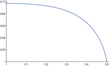
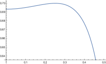
Figure 1. For $S=\tfrac{1}{2}$, the function $g_{\beta}(m)$ with $\beta=1.8$ (left) and $\beta=2.2$ (right). The maximiser $m^{\star}(\beta)$ is positive when $\beta>2$.

Theorem 2.1 (Isotropic Heisenberg model).

For $\Delta=1$ and arbitrary $S\in\tfrac{1}{2}{\mathbb{N}}$, we have

$$\lim_{n\to\infty}\Bigl{\langle}\exp\Bigl{\{}\frac{h}{n}\sum_{i=1}^{n}S_{i}^{(1)}\Bigr{\}}\Bigr{\rangle}_{n,\beta,\Delta=1}^{\rm Heis}=\frac{\sinh(hm^{\star}(\beta))}{hm^{\star}(\beta)},\quad\forall\;h\in{\mathbb{C}}.$$

The proof of this theorem can be found in Section 4.

Concerning symmetry breaking, we expect that the extremal states are labeled by $\vec{a}\in{\mathbb{S}}^{2}$. (The 2-sphere is the orbit of any point on $\Psi_{\beta}$ under the action of the symmetry group $SO(3)$, and $H=SO(2)$). For $\vec{a}\in{\mathbb{S}}^{2}$ we introduce the following Gibbs states:

$$\begin{split}\langle\cdot\rangle_{\vec{a},h}&=\lim_{n\to\infty}\frac{{\operatorname{Tr\,}}[\cdot\,{\rm e}^{-\beta H_{n,\Delta}^{\rm Heis}+h\sum_{i=1}^{n}\vec{a}\cdot\vec{S}_{i}}\,]}{{\operatorname{Tr\,}}[\,{\rm e}^{-\beta H_{n,\Delta}^{\rm Heis}+h\sum_{i=1}^{n}\vec{a}\cdot\vec{S}_{i}}\,]},\\ \langle\cdot\rangle_{\vec{a}}&=\lim_{h\downarrow 0}\langle\cdot\rangle_{\vec{a},h}.\end{split}$$ (2.18)

For $h\neq 0$ the states $\langle\cdot\rangle_{\vec{a},h}$ are extremal by an extension of the Lee-Yang theorem [5, 29]; it is reasonable to expect that the limiting states $\langle\cdot\rangle_{\vec{a}}$ are also extremal, although this has not been proved. (A non-trivial technical issue is whether the limits in (2.18) exist; but we do not worry about it in this discussion.) Defining $m^{\star}(\beta)=\langle S_{i}^{(1)}\rangle_{\vec{e}_{1}}$, we have that

$$\langle S_{i}^{(1)}\rangle_{\vec{a}}=\langle\vec{a}\cdot\vec{S}_{i}\rangle_{\vec{e}_{1}}=a_{1}\langle S_{i}^{(1)}\rangle_{\vec{e}_{1}}=a_{1}m^{\star}(\beta)\,,$$ (2.19)

where $\vec{e}_{1}=(1,0,0)^{T}$ is the unit vector in the $1$-direction. Assuming that (1.3) is correct, we expect that

$$\lim_{n\to\infty}\Big{\langle}\,{\rm e}^{\frac{h}{n}\sum_{i=1}^{n}S_{i}^{(1)}}\,\Big{\rangle}_{n,\beta,\Delta=1}^{\rm Heis}=\frac{1}{4\pi}\int_{{\mathbb{S}}^{2}}\,{\rm e}^{hm^{\star}(\beta)a_{1}}\,{\rm d}\vec{a}\equiv\frac{\sinh(hm^{\star}(\beta))}{hm^{\star}(\beta)}.$$ (2.20)

The right side of (2.20) coincides with the expression in Theorem 2.1; so (1.3) is expected to be correct for this model.

Our next result concerns the Heisenberg Hamiltonians with $\Delta\in[-1,1)$. Models with these Hamiltonians behave just like the xy-model, ($\Delta=0$). For models on the complete graph, this remains true also for $\Delta=-1$. (However, on a bipartite graph (lattice), the model with $\Delta=-1$ is unitarily equivalent to the quantum Heisenberg antiferromagnet whose properties are different from those of the xy-model.) We let $m^{\star}(\beta)$ be the maximiser of the function $g_{\beta}$ in (2.14), as before. Let $I_{0}(x)=\sum_{k\geq 0}\frac{1}{(k!)^{2}}(\frac{x}{2})^{2k}$ be the modified Bessel function.

Theorem 2.2 (Anisotropic Heisenberg model).

For $\Delta\in[-1,1)$ and $S\geq\tfrac{1}{2}$, we have that

$$\lim_{n\to\infty}\Big{\langle}\exp\Bigl{\{}\frac{h}{n}\sum_{i=1}^{n}S_{i}^{(1)}\Bigr{\}}\Big{\rangle}^{\rm Heis}_{n,\beta,\Delta}=I_{0}\bigl{(}hm^{\star}(\beta)\bigr{)}\,,\quad\forall h\in{\mathbb{C}}\,.$$

The proof of this theorem can be found in Section 5. This theorem confirms that the phase transition signals the onset of spontaneous magnetisation in the 1–2 plane. We now introduce

$$\langle\cdot\rangle_{\vec{a}}=\lim_{h\downarrow 0}\lim_{n\to\infty}\frac{{\operatorname{Tr\,}}[\cdot\,{\rm e}^{-\beta H_{n,\Delta}^{\rm Heis}+h\sum_{i=1}^{n}\vec{a}\cdot\vec{S}_{i}}\,]}{{\operatorname{Tr\,}}[\,{\rm e}^{-\beta H_{n,\Delta}^{\rm Heis}+h\sum_{i=1}^{n}\vec{a}\cdot\vec{S}_{i}}\,]}\,,\quad\text{for }\,\vec{a}\perp\vec{e}_{3},\,\,|\vec{a}|=1\,.$$ (2.21)

As in (2.18), these states are limits of extremal states by the Lee-Yang theory, so they should also be extremal. With $m^{\star}(\beta)=\langle S_{i}^{(1)}\rangle_{\vec{e}_{1}}$ as before, according to the heuristics in (1.3), one expects that

$$\lim_{n\to\infty}\Big{\langle}\,{\rm e}^{\frac{h}{n}\sum_{i=1}^{n}S_{i}^{(1)}}\,\Big{\rangle}_{n,\beta,\Delta}^{\rm Heis}=\frac{1}{2\pi}\int_{{\mathbb{S}}^{1}}\,{\rm e}^{hm^{\star}(\beta)a_{1}}\,{\rm d}\vec{a}\equiv I_{0}\bigr{(}hm^{\star}(\beta)\bigl{)}.$$ (2.22)

Since we get exactly what is stated in Theorem 2.2, we are tempted to conclude that the above heuristics are valid.

2.2. Quantum interchange model

We turn to the quantum interchange model. Recall that, for $S=\frac{1}{2}$, this model is equivalent to the Heisenberg model. To avoid overlap with Theorem 2.1, for this model we consider only $S\geq 1$. General values of $S$ are interesting because the pattern of symmetry breaking changes; but the calculations become considerably more difficult.

In order to define the object that plays the rôle of the magnetisation, let $\phi_{\beta}$ be the function $[0,1]^{2S+1}\to{\mathbb{R}}$ given by

$$\phi_{\beta}(x_{1},\dots,x_{2S+1})=\frac{\beta}{2}\Bigl{(}\sum_{i=1}^{2S+1}x_{i}^{2}-1\Bigr{)}-\sum_{i=1}^{2S+1}x_{i}\log x_{i}.$$ (2.23)

We look for maximisers $(x_{1}^{\star},\dots,x_{2S+1}^{\star})$ of $\phi_{\beta}$ under the condition $\sum_{i}x_{i}=1$ and $x_{1}\geq x_{2}\geq\dots\geq x_{2S+1}$. It was understood and proven by Björnberg, see [9, Theorem 4.2], that the answer involves the critical parameter

$$\beta_{\rm c}(S)=\frac{4S}{2S-1}\log(2S),\qquad(S\geq 1).$$ (2.24)

The maximiser is unique and satisfies

$$\begin{split}&x_{1}^{\star}=\dots=x_{2S+1}^{\star}=\tfrac{1}{2S+1},\qquad\text{if }\beta<\beta_{\rm c}(S),\\ &x_{1}^{\star}>x_{2}^{\star}=\dots=x_{2S+1}^{\star},\quad\qquad\text{if }\beta\geq\beta_{\rm c}(S)\end{split}$$ (2.25)

(see Appendix C). The analogue of the magnetisation is defined as

$$z^{\star}(\beta)=\frac{(2S+1)x_{1}^{\star}-1}{2S}=x_{1}^{\star}-x_{2}^{\star}.$$ (2.26)

In the following theorem, $R$ denotes the function

$$R(h_{1},\dotsc,h_{2S+1};x_{1},\dotsc,x_{2S+1})=\det\big{[}e^{h_{i}x_{j}}\big{]}_{i,j=1}^{2S+1}\prod_{1\leq i<j\leq 2S+1}\frac{j-i}{(h_{i}-h_{j})(x_{i}-x_{j})}$$ (2.27)

and if $A$ is an arbitrary $(2S+1)\times(2S+1)$ matrix then $A_{i}:={\mathchoice{\rm 1\mskip-4.0mul}{\rm 1\mskip-4.0mul}{\rm 1\mskip-4.5mul}{\rm 1\mskip-5.0mul}}\otimes\dots\otimes A\otimes\dots\otimes{\mathchoice{\rm 1\mskip-4.0mul}{\rm 1\mskip-4.0mul}{\rm 1\mskip-4.5mul}{\rm 1\mskip-5.0mul}}$, where $A$ occupies the $i$th factor. Note that $R$ is continuous: in the numerator, $\det\big{[}e^{h_{i}x_{j}}\big{]}_{i,j=1}^{\theta}$ is analytic in the variables $h_{i}$ and $x_{i}$, and it is anti-symmetric under permutations of the arguments $h_{i}$ and $x_{i}$, hence it vanishes whenever two or more of the $h_{i}$’s or of the $x_{i}$’s coincide.

Theorem 2.3 (Spin-$S$ quantum interchange model).

For an arbitrary $(2S+1)\times(2S+1)$ matrix $A$, with eigenvalues $h_{1},\dotsc,h_{2S+1}\in{\mathbb{C}}$, we have that

$$\lim_{n\to\infty}\Big{\langle}\exp\Bigl{\{}\frac{1}{n}\sum_{i=1}^{n}A_{i}\Bigr{\}}\Big{\rangle}_{n,\beta}^{\rm int}=R(h_{1},\dotsc,h_{2S+1};x^{\star}_{1},\dotsc,x^{\star}_{2S+1}).$$

We highlight the following two special cases of this result: first, we get that

$$\lim_{n\to\infty}\Big{\langle}\exp\Bigl{\{}\frac{h}{n}\sum_{i=1}^{n}S_{i}^{(1)}\Bigr{\}}\Big{\rangle}_{n,\beta}^{\rm int}=\Bigl{(}\frac{\sinh(\frac{1}{2}hz^{\star})}{\frac{1}{2}hz^{\star}}\Bigr{)}^{2S};$$ (2.28)

second, if $Q$ denotes an arbitrary rank 1 projector, with eigenvalues $1,0,\dotsc,0$, we get

$$\lim_{n\to\infty}\Big{\langle}\exp\Bigl{\{}\frac{h}{n}\sum_{i=1}^{n}Q_{i}\Bigr{\}}\Big{\rangle}_{n,\beta}^{\rm int}=\frac{(2S)!}{(hz^{\star})^{2S}}\,{\rm e}^{\frac{h}{2S+1}(1-z^{\star})}\,\sum_{j=2S}^{\infty}\frac{(hz^{\star})^{j}}{j!}$$ (2.29)

The step from Theorem 2.3 to (2.28) and (2.29) is not immediate; details appear in Sect. 6.

Next, we discuss the heuristics of spontaneous symmetry breaking. The Hamiltonian of the interchange model is invariant under an SU$(2S+1)$-symmetry: Given an arbitrary unitary matrix $U$ on ${\mathbb{C}}^{2S+1}$, let $U_{n}=\otimes_{i=1}^{n}U$; then $U_{n}^{-1}H_{n}^{\rm int}U_{n}=H_{n}^{\rm int}$. As pointed out to us by Robert Seiringer, the extremal states are labeled by rank-1 projections on ${\mathbb{C}}^{2S+1}$, or, equivalently, by the complex projective space ${\mathbb{C}}{\mathbb{P}}^{2S}$ (i.e., by the set of equivalence classes of vectors in ${\mathbb{C}}^{2S+1}$ only differing by multiplication by a complex nonzero number). Given $v\in{\mathbb{C}}^{2S+1}\setminus\{0\}$, let $P^{v}$ denote the orthogonal projection onto $v$, and let $P_{i}^{v}:={\mathchoice{\rm 1\mskip-4.0mul}{\rm 1\mskip-4.0mul}{\rm 1\mskip-4.5mul}{\rm 1\mskip-5.0mul}}\otimes\dots\otimes P^{v}\otimes\dots\otimes{\mathchoice{\rm 1\mskip-4.0mul}{\rm 1\mskip-4.0mul}{\rm 1\mskip-4.5mul}{\rm 1\mskip-5.0mul}}$, where $P^{v}$ occupies the $i$th factor. The extremal states are expected to be given by

$$\langle\cdot\rangle_{v}=\lim_{h\downarrow 0}\lim_{n\to\infty}\frac{{\operatorname{Tr\,}}[\cdot\,{\rm e}^{-\beta H_{n}^{\rm int}+h\sum_{i=1}^{n}P_{i}^{v}}\,]}{{\operatorname{Tr\,}}[\,{\rm e}^{-\beta H_{n}^{\rm int}+h\sum_{i=1}^{n}P_{i}^{v}}\,]}.$$ (2.30)

As $\beta\to\infty$, $\langle\cdot\rangle_{v}$ converges to the expectation defined by the product state $\otimes v$. These product states are ground states of $H_{n}^{\rm int}$, which gives some justification to the claim that the states $\langle\cdot\rangle_{v}$ are extremal. We expect that

$$\lim_{n\to\infty}\Big{\langle}\exp\Bigl{\{}\frac{1}{n}\sum_{i=1}^{n}A_{i}\Bigr{\}}\Big{\rangle}_{n,\beta}^{\rm int}=\int_{{\mathbb{C}}{\mathbb{P}}^{2S}}\,{\rm e}^{\langle A_{1}\rangle_{v}}\,{\rm d}v.$$ (2.31)

We take the state $\langle\cdot\rangle_{e_{1}}$ as the reference state, with vector $v=e_{1}=(1,0,\dots,0)$. At the cost of some redundancy, the integral over $v$ in ${\mathbb{C}}{\mathbb{P}}^{2S}$ can be written as an integral over the space ${\mathcal{U}}(2S+1)$ of unitary matrices on ${\mathbb{C}}^{2S+1}$ with the uniform probability (Haar) measure:

$$\int_{{\mathbb{C}}{\mathbb{P}}^{2S}}\,{\rm e}^{\langle A_{1}\rangle_{v}}\,{\rm d}v=\int_{{\mathcal{U}}(2S+1)}\,{\rm e}^{\langle U_{1}^{-1}A_{1}U_{1}\rangle_{e_{1}}}\,{\rm d}U.$$ (2.32)

Next we consider the restriction of the state $\langle\cdot\rangle_{e_{1}}$ onto operators that only involve the spin at site 1. This restriction can be represented by a density matrix $\rho$ on ${\mathbb{C}}^{2S+1}$ such that

$$\langle A_{1}\rangle_{e_{1}}={\operatorname{Tr\,}}_{{\mathbb{C}}^{2S+1}}(A\rho).$$ (2.33)

In all bases where $e_{1}=(1,0,\dots,0)$, the matrix $\rho$ is diagonal with entries $(x_{1}^{\star},\dots,x_{2S+1}^{\star})$ on the diagonal, where

$$x_{i}^{\star}={\operatorname{Tr\,}}(P^{e_{i}}\rho)=\langle P_{1}^{e_{i}}\rangle_{e_{1}}.$$ (2.34)

It is clear that $x_{2}^{\star}=\dots=x_{2S+1}^{\star}$, and one should expect that $x_{1}^{\star}$ is larger than or or equal to $x_{2}^{*}$. Heuristic arguments suggest that

$$\lim_{n\to\infty}\Big{\langle}\exp\Bigl{\{}\frac{1}{n}\sum_{i=1}^{n}A_{i}\Bigr{\}}\Big{\rangle}_{n,\beta}^{\rm int}=\int_{{\mathcal{U}}(2S+1)}\,{\rm e}^{{\operatorname{Tr\,}}(AU\rho U^{-1})}\,{\rm d}U.$$ (2.35)

By the Harish-Chandra–Itzykson-Zuber formula [16], the right-hand-side of (2.35) is equal to $R(h_{1},\dots,h_{2S+1};x_{1}^{\star},\dots,x_{2S+1}^{\star})$ which agrees with the right-hand-side in Theorem 2.3.

2.3. Critical exponents for the Heisenberg model

Relatively minor extensions of our calculations for the Heisenberg model ($\Delta=1$) enable us to determine some critical exponents for that model on the complete graph. To state our results, we introduce the pressure

$$p(\beta,h)=\lim_{n\to\infty}\tfrac{1}{n}\log{\operatorname{Tr\,}}\big{(}\exp(-\beta H^{\mathrm{Heis}}_{n,\Delta=1}+h\textstyle\sum_{i=1}^{n}S^{(1)}_{i})\big{)}$$ (2.36)

(more accurately, this is $(-\beta)$ times the free energy; “pressure” is used by analogy to the Ising model, where it is justified by the lattice-gas interpretation). Next, we consider the magnetization and susceptibility

$$m(\beta,h)=\frac{\partial p}{\partial h},\qquad\chi(\beta)=\frac{\partial m}{\partial h}\Big{|}_{h=0}$$ (2.37)

and the transverse susceptibility

$$\chi^{\perp}_{n}(\beta,h)=\frac{1}{n}\sum_{1\leq i<j\leq n}\frac{{\operatorname{Tr\,}}\big{(}S^{(2)}_{i}S^{(2)}_{j}\,{\rm e}^{-\beta H^{\mathrm{Heis}}_{n}+h\sum_{i=1}^{n}S^{(1)}_{i}}\,\big{)}}{{\operatorname{Tr\,}}\big{(}\,{\rm e}^{-\beta H^{\mathrm{Heis}}_{n}+h\sum_{i=1}^{n}S^{(1)}_{i}}\,\big{)}}$$ (2.38)

as well as the limit $\chi^{\perp}(\beta,h)=\lim_{n\to\infty}\chi^{\perp}_{n}(\beta,h)$ (where we extract a converging subsequence if necessary).

The following theorem is proven in Section 7. Recall the function $g_{\beta}(m)$, $0\leq m\leq S$, given in (2.14) (which reduces to (2.17) for $S=\tfrac{1}{2}$). We write $f\sim g$ if $f/g$ converges to a positive constant.

Theorem 2.4.

For the spin-$S\geq\tfrac{1}{2}$ Heisenberg models the following formulae hold true.

(i) Pressure:

$$p(\beta,h)=\max_{0\leq m\leq S}\big{(}g_{\beta}(m)+hm\big{)}\,.$$ (2.39)

(ii) Critical Exponents:

$$\begin{split}m^{\star}(\beta)\underset{\beta\downarrow\beta_{\mathrm{c}}}{\sim}(\beta-\beta_{\mathrm{c}})^{1/2}\,,\quad\chi(\beta)\underset{\beta\uparrow\beta_{\mathrm{c}}}{\sim}(\beta_{\mathrm{c}}-\beta)^{-1}\,,\quad m(\beta_{\mathrm{c}},h)\underset{h\downarrow 0}{\sim}h^{1/3}\,,\end{split}$$ (2.40)

and

$$\chi^{\perp}(\beta_{\mathrm{c}},h)\underset{h\downarrow 0}{\sim}h^{-2/3}\,,\qquad\chi^{\perp}(\beta,h)\underset{h\downarrow 0}{\sim}h^{-1}\,,\mbox{ for }\,\beta>\beta_{\mathrm{c}}\,.$$ (2.41)

We note that the critical exponents (2.40) are exactly the same as for the classical spin-$\tfrac{1}{2}$ Curie–Weiss (Ising) model, which has Hamiltonian $H_{n}=-\frac{2}{n}\sum_{i<j}S^{(1)}_{i}S^{(1)}_{j}$, see e.g. [11, Ch. 2]. Moreover, in the case $S=\tfrac{1}{2}$ the pressure (2.39) for the quantum Heisenberg model equals that of the Curie–Weiss model, see [11, Thm 2.8]. Nonetheless, the models are not identical, as shown by Theorem 2.1: for the Curie–Weiss model a simple calculation shows that $\langle\,{\rm e}^{\tfrac{h}{n}\sum_{i}S^{(1)}_{i}}\,\rangle\to\cosh(hm^{\star})$.

In proving (2.41) we will use general inequalities relating the transverse susceptibility to the magnetization, which follow from Ward-identities and the Falk–Bruch inequality. For details, see Section 7.

3. Random loop representations

The Gibbs states of quantum spin systems can be described with the help of Feynman–Kac expansions. In some cases these expansions can be represented as probability measures on sets of loop configurations. Such cases include Tóth’s random interchange representation for the spin-$\frac{1}{2}$ Heisenberg ferromagnet. (An early version of this representation is due to Powers [25]; it was independently proposed by Tóth in [31], with a precise formulation and interesting applications.) Another useful representation is Aizenman and Nachtergaele’s loop model for the spin-$\frac{1}{2}$ Heisenberg antiferromagnet, and models of arbitrary spins where interactions are given by projectors onto spin singlets [2]. Nachtergaele extended these representations to Heisenberg models of arbitrary spin [22]. A synthesis of the Tóth- and the Aizenman–Nachtergaele loop models, which allows one to describe the spin-$\frac{1}{2}$ xy-model and a spin-1 nematic model, was proposed in [33].

These models are interesting from the point of view of probability theory and they are relevant here because the joint distribution of loop lengths turns out to be related to the extremal state decomposition of the corresponding quantum systems. Indeed, some characteristic functions for the loop lengths are equal to the Laplace transforms of the measure on the set of extremal states.

The loop models considered in this paper can be defined on any graph $\Gamma$, and involve one-dimensional loops immersed in the space $\Gamma\times[0,\beta]$. Quantum-mechanical correlations can be expressed in terms of probabilities for loop connectivity. The lengths of the loops, rescaled by an appropriate fractional power of the spatial volume, are expected to display a universal behavior: there are macroscopic and microscopic loops, and the limiting joint distribution of the lengths of macroscopic loops is expected to be the Poisson–Dirichlet (PD) distribution that originally appeared in the work of Kingman [17]. This distribution is illustrated in Fig. 2.

Figure 2. Conjectured form for typical partition given by loop lengths in dimensions $d\geq 3$. For some $z^{\star}\in[0,1]$, the partition in $[0,z^{\star}]$ follows a Poisson-Dirichlet distribution; the partition in the interval $[z^{\star},1]$ consists of microscopic elements.

The Poisson–Dirichlet distribution, denoted by PD($\theta$), with $\theta>0$ arbitrary, can be defined via the following ‘stick-breaking’ construction: Let $B_{1},B_{2},\dotsc$ be independent Beta(1,$\theta$)-distributed random variables, thus ${\mathbb{P}}(B_{i}>t)=(1-t)^{\theta}$ for $t\in[0,1]$. Consider the sequence $Y=(Y_{1},Y_{2},\dotsc)$ given by

$$Y_{1}=B_{1};\quad Y_{2}=B_{2}(1-B_{1});\quad\dotsc\quad Y_{n}=B_{n}\prod_{i=1}^{n-1}(1-B_{i}).$$ (3.1)

The vector $X$ obtained by ordering the elements of $Y$ by size has the PD($\theta$)-distribution. Note that $\sum_{i\geq 1}X_{i}=1$ with probability 1, hence the $X_{i}$ may be regarded as giving a partition of the interval $[0,1]$. To obtain a partition of an interval $[0,z^{\star}]$ as in Fig. 2 one simply rescales $X$ by $z^{\star}$. For future reference we note here the following formula, which will turn out to be relevant for the spin-systems considered in this paper. In [35, Eq. (4.18)] it is shown that

$${\mathbb{E}}_{{\rm PD}(\theta)}\biggl{[}\prod_{i\geq 1}\cosh(hX_{i})\biggr{]}=\frac{1}{\Gamma(\theta/2)}\sum_{k\geq 0}\frac{\Gamma(\theta/2+k)}{k!\,\Gamma(\theta+2k)}h^{2k}.$$ (3.2)

The Poisson–Dirichlet distribution first appeared in the study of the random interchange model (transposition-shuffle) on the complete graph. David Aldous formulated a conjecture concerning the convergence of the rescaled loop sizes to PD(1), and he explained the heuristics; Schramm then provided a proof [26] of Aldous’ conjecture. Models on the complete graph are easier to analyse than the corresponding models on a lattice ${\mathbb{Z}}^{d}$, $d\geq 3$; but the heuristics for the latter models is remarkably similar to the one for the former models; see [13, 35]. The ideas sketched here are confirmed by the results of numerical simulations of various loop soups, including lattice permutations [14], loop O(N)-models [23], and the random interchange model [6].

3.1. Spin-$\frac{1}{2}$ models

We begin by describing the loop representations of the Heisenberg models with spin $S=\tfrac{1}{2}$. These representations are quite well known and contain many of the essential features, but without some of the complexities that appear for larger spin.

We pick a real number $u\in[0,1]$. Let $\Gamma=K_{n}$ be the complete graph, with vertices $V_{n}=\{1,\dotsc,n\}$ and edges $E_{n}=\big{\{}\{i,j\}:1\leq i<j\leq n\big{\}}$. With each edge we associate an independent Poisson point process on the time interval $[0,\beta/n]$ with two kinds of outcomes: ‘crosses’ occur with intensity $u$ and ‘double bars’ occur with intensity $1-u$. We let $\rho_{n,\beta,u}$ denote the law of the Poisson point processes. Given a realization $\omega$, the loop containing the point $(v,t)\in K_{n}\times[0,\beta/n]$ is obtained by moving vertically until meeting a cross or a double bar, then crossing the edge to the other vertex, and continuing in the same vertical direction, for a cross, while continuing in the opposite direction, for a double bar; see Fig. 3. Periodic boundary conditions are imposed in the vertical direction at $0$ and $\beta/n$. In the following, ${\mathcal{L}}(\omega)$ denotes the set of all such loops.

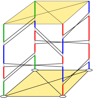
Figure 3. A realization on the complete graph $K_{4}$ with three loops; the green loop has length 2, the red and blue loops have length 1.

Let

$${\mathbb{P}}_{n,\beta,2,u}({\rm d}\omega)=\frac{1}{Z(n,\beta,2,u)}2^{|{\mathcal{L}}(\omega)|}\rho_{n,\beta,u}({\rm d}\omega),$$ (3.3)

where the normalisation $Z(n,\beta,2,u)=\int 2^{|{\mathcal{L}}(\omega)|}\rho_{n,\beta,u}({\rm d}\omega)$ is the partition function. By ${\mathbb{E}}_{n,\beta,2,u}$ we denote an expectation with respect to this probability measure.

We define the length of a loop as the number of points $(i,0)$ that it contains; i.e., the length of a loop is the number of sites at level $0\in[0,\beta/n]$ visited by the loop. (According to this definition, there are loops of length 0.) Given a realisation $\omega$, let $\ell_{1}(\omega),\ell_{2}(\omega),\dots$ be the lengths of the loops in decreasing order. We have that $\sum_{i\geq 1}\ell_{i}(\omega)=n$, for an arbitrary $\omega$. Thus, $\bigl{(}\frac{\ell_{1}(\omega)}{n},\frac{\ell_{2}(\omega)}{n},\dots\bigr{)}$ is a random partition of the interval $[0,1]$. We expect it to resemble the partition depicted in Fig. 2.

One manifestation of the connection between the loop-model and the spin system is the following identity, valid for $\Delta=2u-1$:

$$\langle\,{\rm e}^{\frac{h}{n}\sum_{i}S_{i}^{(1)}}\,\rangle^{\mathrm{Heis}}_{n,\beta,\Delta}={\mathbb{E}}_{n,\beta,2,u}\biggl{[}\prod_{i\geq 1}\cosh\Bigl{(}\frac{h\ell_{i}(\omega)}{2n}\Bigr{)}\biggr{]}.$$ (3.4)

This is a special case of (3.19) below.

3.2. Heisenberg models with arbitrary spins

An extension of the loop representation for the Heisenberg ferromagnet (and antiferromagnet, and further interactions) with arbitrary spin was proposed by Bruno Nachtergaele [22]. As in [33] it can be generalised to include asymmetric Heisenberg models. We first describe this representation and state our results about the lengths of the loops. Afterwards, we will outline the derivation of this representation from models of spins.

We introduce a model where every site is replaced by $2S$ “pseudo-sites”. Let $\widetilde{K}_{n}$ be the graph whose vertices are the pseudo-sites $\bigl{\{}(i,\alpha):i\in\{1,\dots,n\},\alpha\in\{1,\dots,2S\}\bigr{\}}$ and whose edges are given by

$$\widetilde{\mathcal{E}}_{n}=\bigl{\{}\{(i,\alpha),(j,\alpha^{\prime})\}:1\leq i<j\leq n,1\leq\alpha,\alpha^{\prime}\leq 2S\bigr{\}}.$$ (3.5)

We require the following ingredients:

• A uniformly random permutation $\sigma$ of the pseudo-sites at each vertex; namely, $\sigma=(\sigma_{i})_{i=1}^{n}$, where the $\sigma_{i}$ are independent, uniform permutations of $2S$ elements.

• (Independently of $\sigma$) the result $\omega$ of independent Poisson point processes in the time interval $[-\frac{\beta}{2n},\frac{\beta}{2n}]$, for every edge of $\widetilde{\mathcal{E}}_{n}$, where crosses have intensity $u$ and double bars have intensity $1-u$.

Let $\widetilde{\rho}_{n,\beta,u}$ denote the measure for the Poisson point process. The measure on the set of permutations is just the counting measure. Loops are defined as before, except that the permutations rewire the threads between times $\frac{\beta}{2n}$ and $-\frac{\beta}{2n}$. An illustration is given in Fig. 4.

Figure 4. Loop representation for Heisenberg models with spins $S=\frac{3}{2}$. The original graph is modified so each site is now hosting $2S=3$ pseudo-sites. There are random permutations of pseudo-sites between times $\frac{\beta}{2n}$ and $-\frac{\beta}{2n}$. As before, there is an overall factor $2^{\#{\rm loops}}$. In the realisation above, one loop is highlighted (it has length 3) and there are three other loops (of length 0, 4, and 5).

The probability measure relevant for the following considerations is the following measure:

$$\widetilde{\mathbb{P}}_{n,\beta,2,u}(\sigma,{\rm d}\omega)=\frac{1}{\widetilde{Z}(n,\beta,2,u)}2^{|{\mathcal{L}}(\sigma,\omega)|}\widetilde{\rho}_{n,\beta,2,u}({\rm d}\omega).$$ (3.6)

Expectation with respect to $\widetilde{\mathbb{P}}_{n,\beta,2,u}(\sigma,{\rm d}\omega)$ is denoted by $\tilde{\mathbb{E}}_{n,\beta,2,u}$. We define the length of a loop as the number of sites at time 0 visited by it. For any realisation $(\sigma,\omega)$, we have that $\sum_{i\geq 1}\ell_{i}(\sigma,\omega)=2Sn$.

As we will explain below, this loop model provides a probabilistic representation of the Heisenberg model with $\Delta=2u-1$. The two parts of the following theorem are equivalent to Theorems 2.1 and 2.2, respectively.

Theorem 3.1.

Let $z^{\star}=m^{\star}(\beta)/S$ with $m^{\star}(\beta)$ defined above in Eq. (2.15). For any $h\in{\mathbb{C}}$, we have that

$$\lim_{n\to\infty}\tilde{\mathbb{E}}_{n,\beta,2,u}\biggl{[}\prod_{i\geq 1}\cosh\Bigl{(}\frac{h\ell_{i}(\sigma,\omega)}{2Sn}\Bigr{)}\biggr{]}=\begin{cases}\sinh(hz^{\star})/hz^{\star},&\text{if }u=1,\\ I_{0}(hz^{\star}),&\text{if }u\in[0,1).\end{cases}$$

We note that the limiting quantities agree with the corresponding expectations with respect to the Poisson–Dirichlet distributions; more precisely PD(2), for $u=1$, and PD(1), for $u<1$. Indeed, setting $\theta=2$ in (3.2), we find that

$${\mathbb{E}}_{{\rm PD}(2)}\biggl{[}\prod_{i\geq 1}\cosh(hX_{i})\biggr{]}=\sum_{k\geq 0}\frac{h^{2k}}{(2k+1)!}=\frac{\sinh(h)}{h}\,,$$ (3.7)

while setting $\theta=1$ yields

$${\mathbb{E}}_{{\rm PD}(1)}\biggl{[}\prod_{i\geq 1}\cosh(hX_{i})\biggr{]}=\frac{1}{\Gamma(\tfrac{1}{2})}\sum_{k\geq 0}\frac{\Gamma(k+\tfrac{1}{2})}{k!(2k)!}h^{2k}=I_{0}(h).$$ (3.8)

Next, we explain how to derive this loop model from quantum spin systems. This will show that Theorem 3.1 is equivalent to Theorem 2.1.

Following Nachtergaele [22], we consider the Hilbert space

$$\widetilde{\mathcal{H}}_{n}=\otimes_{i=1}^{n}\otimes_{\alpha=1}^{2S}{\mathbb{C}}^{2}.$$ (3.9)

On $\otimes_{\alpha=1}^{2S}{\mathbb{C}}^{2}$, let $P^{\rm sym}$ denote the projection onto the symmetric subspace; i.e.,

$$P^{\rm sym}=\frac{1}{(2S)!}\sum_{\sigma\in{\mathcal{S}}_{2S}}U(\sigma),$$ (3.10)

where the unitary matrix $U(\sigma)$ is the representative of the permutation $\sigma$,

$$U(\sigma)|\varphi_{1}\rangle\otimes\dots\otimes|\varphi_{2S}\rangle=|\varphi_{\sigma(1)}\otimes\dots\otimes|\varphi_{\sigma(2S)}\rangle.$$ (3.11)

One can check that ${\rm rank}(P^{\rm sym})=2S+1$. Let $P_{n}^{\rm sym}=\otimes_{i=1}^{n}P^{\rm sym}$ and $\widetilde{\mathcal{H}}_{n}^{\rm sym}=P_{n}^{\rm sym}\widetilde{\mathcal{H}}_{n}$. Since ${\rm dim}\,\widetilde{\mathcal{H}}_{n}^{\rm sym}=(2S+1)^{n}$, there is an embedding

$$\iota:{\mathcal{H}}_{n}=({\mathbb{C}}^{2S+1})^{\otimes n}\to\widetilde{\mathcal{H}}_{n}=\widetilde{\mathcal{H}}_{n}^{\rm sym}\oplus(\widetilde{\mathcal{H}}_{n}^{\text{sym}})^{\perp},$$ (3.12)

with the property that

$$A\mapsto\iota(A)=A\oplus 0.$$ (3.13)

With each pseudo-site $(i,\alpha)$ one associates spin operators $S_{i,\alpha}^{(j)}$, $j=1,2,3$, given by ($\frac{1}{2}\times$) Pauli matrices, tensored by the identity. Let

$$R_{i}^{(j)}=P_{n}^{\rm sym}\sum_{\alpha=1}^{2S}S_{i,\alpha}^{(j)}.$$ (3.14)

Then $\iota(S_{i}^{(j)})=R_{i}^{(j)}$. The Hamiltonian is

$$\begin{split}\widetilde{H}_{n}&=-2\sum_{1\leq i<j\leq n}\bigl{(}R_{i}^{(1)}R_{j}^{(1)}+R_{i}^{(2)}R_{j}^{(2)}+\Delta R_{i}^{(3)}R_{j}^{(3)}\bigr{)}\\ &=-2P_{n}^{\rm sym}\sum_{\begin{subarray}{c}1\leq i<j\leq n\\ 1\leq\alpha,\alpha^{\prime}\leq 2S\end{subarray}}\bigl{(}S_{i,\alpha}^{(1)}S_{j,\alpha^{\prime}}^{(1)}+S_{i,\alpha}^{(2)}S_{j,\alpha^{\prime}}^{(2)}+\Delta S_{i,\alpha}^{(3)}S_{j,\alpha^{\prime}}^{(3)}\bigr{)}.\end{split}$$ (3.15)

Notice that $\widetilde{H}_{n}=\iota(H_{n})$. We introduce the transposition operator $T_{(i,\alpha),(j,\alpha^{\prime})}$ and the “double bar operator” $Q_{(i,\alpha),(j,\alpha^{\prime})}$; in the basis where $S_{i,\alpha}^{(1)}=\frac{1}{2}\bigl{(}\begin{smallmatrix}1&0\\ 0&-1\end{smallmatrix}\bigr{)}$, it has matrix elements

$$\langle a|\otimes\langle b|Q_{(i,\alpha),(j,\alpha^{\prime})}|c\rangle\otimes|d\rangle=\delta_{a,b}\delta_{c,d}.$$ (3.16)

Let $u=\frac{1}{2}(\Delta+1)$; we have that

$$2\bigl{(}S_{i,\alpha}^{(1)}S_{j,\alpha^{\prime}}^{(1)}+S_{i,\alpha}^{(2)}S_{j,\alpha^{\prime}}^{(2)}+\Delta S_{i,\alpha}^{(3)}S_{j,\alpha^{\prime}}^{(3)}\bigr{)}=uT_{(i,\alpha),(j,\alpha^{\prime})}+(1-u)Q_{(i,\alpha),(j,\alpha^{\prime})}-\tfrac{1}{2}.$$ (3.17)

The loop expansion can be carried out as in [31, Theorem 2], [2, Proposition 2.1 (iii)], [22], and [33, Section III. B]. In order to formulate the relation between quantum spins and random loops, we need the notion of space-time spin configurations ${\boldsymbol{s}}=\bigl{(}s_{i,\alpha}(t)\bigr{)}$, taking values in $\{-\frac{1}{2},\frac{1}{2}\}$, and indexed by integers $1\leq i\leq n$, $1\leq\alpha\leq 2S$ and by real numbers $0\leq t<\beta$. Given a realisation $(\sigma,\omega)$, we let $\Sigma(\sigma,\omega)$ denote the set of space-time spin configurations ${\boldsymbol{s}}$ that take constant values along the loops of $(\sigma,\omega)$, and that are left-continuous at the points of discontinuity. Notice that

$$|\Sigma(\sigma,\omega)|=2^{|{\mathcal{L}}(\sigma,\omega)|}.$$ (3.18)

Proposition 3.2.

Let $\Delta=2u-1$. For all functions $f:[-\frac{1}{2},\frac{1}{2}]^{2Sn}\to{\mathbb{C}}$ that have convergent Taylor series, we have

$$\bigl{\langle}f(\{S^{(1)}_{i,\alpha}\})\bigr{\rangle}_{n,\beta,\Delta}=\frac{1}{\widetilde{Z}(n,\beta,2,u)}\int\widetilde{\rho}_{n,\beta,2,u}({\rm d}\omega)\sum_{\sigma}\sum_{{\boldsymbol{s}}\in\Sigma(\sigma,\omega)}f\bigl{(}\{s_{i,\alpha}(0)\}\bigr{)}.$$

It immediately follows from this proposition that

$$\Bigl{\langle}\exp\Bigl{\{}\frac{h}{n}\sum_{i=1}^{n}S_{i}^{(1)}\Bigr{\}}\Bigr{\rangle}_{n,\beta,\Delta}=\tilde{\mathbb{E}}_{n,\beta,2,u}\biggl{[}\prod_{i\geq 1}\cosh\Bigl{(}\frac{h\ell_{i}(\sigma,\omega)}{2n}\Bigr{)}\biggr{]}.$$ (3.19)

In particular, Theorem 3.1 follows from Theorems 2.1 and 2.2, which are proven in Sects. 4 and 5, respectively.

3.3. The quantum interchange model

The interchange model has a loop-representation very similar to Tóth’s representation of the spin-$\tfrac{1}{2}$ Heisenberg ferromagnet, which was described in Section 3.1. Indeed, the measure appropriate for this model is obtained by replacing Eq. (3.3) by

$${\mathbb{P}}_{n,\beta,\theta,u=1}({\rm d}\omega)=\frac{1}{Z(n,\beta,\theta,1)}\theta^{|{\mathcal{L}}(\omega)|}\rho_{n,\beta,1}({\rm d}\omega),$$ (3.20)

where $\theta=2S+1$. Note that we set $u=1$, meaning we have only crosses (no double-bars), and that we replace the weight $2^{|\mathcal{L}(\omega)|}$ by $\theta^{|\mathcal{L}(\omega)|}$.

We write $\mathbf{h}=(h_{1},\dotsc,h_{\theta})$ and

$$q_{\mathbf{h}}(t)=\tfrac{1}{\theta}\big{(}e^{h_{1}t}+\dotsb+e^{h_{\theta}t}\big{)}.$$ (3.21)

Recall the function $R$ defined in (2.27).

Theorem 3.3.

For any fixed $\mathbf{h}=(h_{1},\dotsc,h_{\theta})$ we have, as $n\to\infty$,

$${\mathbb{E}}_{n,\beta,\theta,1}\Big{[}\prod_{i\geq 1}q_{\mathbf{h}}(\tfrac{1}{n}\ell_{i})\Big{]}\to R(h_{1},\dotsc,h_{\theta};x_{1}^{\star},\dotsc,x_{\theta}^{\star}),$$ (3.22)

where $(x^{\star}_{1},\dotsc,x_{\theta}^{\star})$ is the maximizer of $\phi_{\beta}(\cdot)$, as above.

Again, the result is equivalent to a statement about the spin system. In this case it is equivalent to Theorem 2.3, since we have the identity (that follows from Proposition 3.2)

$$\Big{\langle}\exp\Bigl{\{}\frac{1}{n}\sum_{i=1}^{n}A_{i}\Bigr{\}}\Big{\rangle}_{n,\beta}^{\rm int}={\mathbb{E}}_{n,\beta,\theta,1}\Big{[}\prod_{i\geq 1}q_{\mathbf{h}}(\tfrac{1}{n}\ell_{i})\Big{]}$$ (3.23)

if $A$ has eigenvalues $h_{1},\dotsc,h_{\theta}$.

The two special cases (2.28) and (2.29) have the following counterparts. We use the notation

$$q_{S}(t)=\tfrac{1}{\theta}\big{(}e^{-St}+e^{-(S-1)t}+\dotsb+e^{St}\big{)}=\frac{\sinh(\tfrac{\theta}{2}t)}{\theta\sinh(\tfrac{1}{2}t)},$$ (3.24)

which corresponds to $h_{i}=(-S+i-1)$. For all $h\in{\mathbb{C}}$, we have that

$$\lim_{n\to\infty}{\mathbb{E}}_{n,\beta,\theta,1}\Big{[}\displaystyle\prod_{i\geq 1}q_{S}(\tfrac{h}{n}\ell_{i})\Big{]}=\Big{[}\frac{\sinh(\tfrac{1}{2}hz^{\star})}{\tfrac{1}{2}hz^{\star}}\Big{]}^{2S},$$ (3.25)

and

$$\lim_{n\to\infty}{\mathbb{E}}_{n,\beta,\theta,1}\Big{[}\prod_{i\geq 1}\tfrac{1}{\theta}(e^{h\ell_{i}/n}+\theta-1)\Big{]}=\exp\big{(}\tfrac{h}{\theta}(1-z^{\star})\big{)}\frac{\sum_{j=\theta-1}^{\infty}\tfrac{1}{j!}(hz^{\star})^{j}}{\tfrac{1}{(\theta-1)!}(hz^{\star})^{\theta-1}}.$$ (3.26)

Moreover, the limiting quantities agree with the corresponding Poisson–Dirichlet expectations, in this case PD($\theta$). In Appendix D we show that

$$\mathbb{E}_{\mathrm{PD}(\theta)}\Big{[}\prod_{i\geq 1}q_{\mathbf{h}}(z^{\star}X_{i})\Big{]}=\exp\big{(}-\tfrac{1-z^{\star}}{\theta}\textstyle\sum_{i}h_{i}\big{)}R(h_{1},\dotsc,h_{\theta};x_{1}^{\star},\dotsc,x_{\theta}^{\star}).$$ (3.27)

In particular,

$${\mathbb{E}}_{{\rm PD}(\theta)}\biggl{[}\prod_{i\geq 1}q_{S}(hX_{i})\biggr{]}=\Big{[}\frac{\sinh(\tfrac{1}{2}h)}{\tfrac{1}{2}h}\Big{]}^{2S},\quad\mbox{for }\theta=2S+1$$ (3.28)

and

$${\mathbb{E}}_{{\rm PD}(\theta)}\biggl{[}\prod_{i\geq 1}\tfrac{1}{\theta}(\,{\rm e}^{hX_{i}}\,+\theta-1)\biggr{]}=\frac{\sum_{j=\theta-1}^{\infty}\tfrac{1}{j!}h^{j}}{\tfrac{1}{(\theta-1)!}h^{\theta-1}}.$$ (3.29)

4. Isotropic Heisenberg Model – Proof of Theorem 2.1

The proof uses standard facts about addition of angular momenta, which for the reader’s convenience are summarised in Appendix A. We also use a simple result about convergence of ratios of sums where the terms are of exponentially large size, Lemma B.1 in Appendix B. To lighten our notation, we use the shorthand $\vec{\Sigma}=(\Sigma^{(1)},\Sigma^{(2)},\Sigma^{(3)})=\sum_{i=1}^{n}\vec{S}_{i}$ for the total spin, and $\vec{\Sigma}^{2}=(\Sigma^{(1)})^{2}+(\Sigma^{(2)})^{2}+(\Sigma^{(3)})^{2}$. Note that $H^{\mathrm{Heis}}_{n,\beta,\Delta}=-\frac{1}{n}\vec{\Sigma}^{2}+\frac{1}{n}(1-\Delta)(\Sigma^{(3)})^{2}$, in particular $H^{\mathrm{Heis}}_{n,\beta,\Delta=1}=-\frac{1}{n}\vec{\Sigma}^{2}$

Let $L_{M,n}$ be the multiplicity of $M$ as an eigenvalue of $\Sigma^{(3)}$ given in Proposition A.1. To prove Theorem 2.1, the main step is to obtain the asymptotic value of $L_{M,n}-L_{M+1,n}$ for large $M,n$. Recall the definitions of $\eta(x)$ and $x^{\star}(m)$ in Eqs (2.10) and (2.12) (note that $x^{\star}(m)$ has the same sign as $m$).

Proposition 4.1.

For $m\in(-S,S)$,

$$L_{\lfloor mn\rfloor,n}-L_{\lfloor mn\rfloor+1,n}=\frac{(1-\,{\rm e}^{-x^{\star}(m)}\,)\bigl{(}1+o(1)\bigr{)}}{\sqrt{2\pi\eta^{\prime\prime}(x^{\star}(m))\,n}}\,{\rm e}^{n[\eta(x^{\star}(m))-mx^{\star}(m)]}\,\,,\,\text{ as }\,n\rightarrow\infty\,.$$

Proof.

We consider the generating function

$$\Phi(z,n)=\sum_{M=-Sn}^{Sn}z^{M+Sn}L_{M,n}=(1+z+\dots+z^{2S})^{n}.$$ (4.1)

Here we used (A.2). By Cauchy’s formula,

$$L_{M,n}=\frac{1}{(M+Sn)!}\frac{{\rm d}^{M+Sn}}{{\rm d}z^{M+Sn}}\Phi(z,n)\Big{|}_{z=0}=\frac{1}{2\pi{\rm i}}\oint\frac{(1+z+\dots+z^{2S})^{n}}{z^{M+Sn}}\frac{{\rm d}z}{z},$$ (4.2)

where integration is along a contour that surrounds the origin. We choose the contour to be a circle of radius $\,{\rm e}^{x}\,$, $x\in{\mathbb{R}}$. Then, assuming that $mn$ is an integer, we have

$$\begin{split}L_{mn,n}-L_{mn+1,n}&=\frac{1}{2\pi}\int_{-\pi}^{\pi}\biggl{[}\frac{1+\,{\rm e}^{x+{\rm i}\varphi}\,+\dots+\,{\rm e}^{2S(x+{\rm i}\varphi)}\,}{\,{\rm e}^{(m+S)(x+{\rm i}\varphi)}\,}\biggr{]}^{n}\big{(}1-\,{\rm e}^{-(x+{\rm i}\varphi)}\,\big{)}{\rm d}\varphi\\ &=\frac{1}{2\pi}\int_{-\pi}^{\pi}\big{(}1-\,{\rm e}^{-(x+{\rm i}\varphi)}\,\big{)}\,{\rm e}^{n[\Upsilon_{m}(x+{\rm i}\varphi)]}\,{\rm d}\varphi,\end{split}$$ (4.3)

where

$$\Upsilon_{m}(x+{\rm i}\varphi)=\log\Big{(}\frac{1+\,{\rm e}^{x+{\rm i}\varphi}\,+\dots+\,{\rm e}^{2S(x+{\rm i}\varphi)}\,}{\,{\rm e}^{(m+S)(x+{\rm i}\varphi)}\,}\Big{)}=\log\Big{(}\frac{\sinh(\frac{2S+1}{2}(x+{\rm i}\varphi))}{\sinh(\frac{1}{2}(x+{\rm i}\varphi))}\,{\rm e}^{-m(x+{\rm i}\varphi)}\,\Big{)}.$$ (4.4)

The latter identity follows easily from the formula for geometric series. It is clear from the first expression that ${\rm Re}\Upsilon_{m}(x+{\rm i}\varphi)$ attains its maximum at $\varphi=0$, for each fixed $x$. Furthermore, we have that $\Upsilon_{m}(x)=\eta(x)-mx$, so the minimum of $\Upsilon(x)$ along the real line satisfies the equation $\eta^{\prime}(x)=m$. As observed before, the unique solution is $x^{\star}(m)$. A standard saddle-point argument then yields

$$\begin{split}L_{mn,n}-L_{mn+1,n}&=\frac{1}{2\pi}\,{\rm e}^{n\Upsilon_{m}(x^{\star}(m))}\,\int_{-\pi}^{\pi}\big{(}1-\,{\rm e}^{-(x+{\rm i}\varphi)}\,\big{)}\,{\rm e}^{n[\Upsilon_{m}(x^{\star}(m)+{\rm i}\varphi)-\Upsilon_{m}(x^{\star}(m))]}\,{\rm d}\varphi\\ &=\bigl{(}1+o(1)\bigr{)}\big{(}1-\,{\rm e}^{-x^{\star}(m)}\,\big{)}\,{\rm e}^{n\Upsilon_{m}(x^{\star}(m))}\,\int_{-\infty}^{\infty}\,{\rm e}^{-\frac{1}{2}n\Upsilon_{m}^{\prime\prime}(x^{\star}(m))\,\varphi^{2}}\,{\rm d}\varphi\\ &=\frac{\big{(}1-\,{\rm e}^{-x^{\star}(m)}\,\big{)}\bigl{(}1+o(1)\bigr{)}}{\sqrt{2\pi\Upsilon_{m}^{\prime\prime}(x^{\star}(m))\,n}}\,{\rm e}^{n\Upsilon_{m}(x^{\star}(m))}\,.\end{split}$$ (4.5)

Since $\Upsilon_{m}^{\prime\prime}(x)=\eta^{\prime\prime}(x)$, the proposition follows. ∎

With this result in hand, the proof of Theorem 2.1 is straightforward:

Proof of Theorem 2.1.

We will write $\langle\cdot\rangle$ for $\langle\cdot\rangle^{\mathrm{Heis}}_{n,\beta,\Delta=1}$.We assume that $Sn$ is an integer; (the case of half-integer values being almost identical). Using Proposition A.1, we get

$$\begin{split}\bigl{\langle}\,{\rm e}^{\frac{h}{n}\Sigma^{(1)}}\,\bigr{\rangle}=\bigl{\langle}\,{\rm e}^{\frac{h}{n}\Sigma^{(3)}}\,\bigr{\rangle}&=\frac{\displaystyle\sum_{J=0}^{Sn}\big{(}L_{J,n}-L_{J+1,n}\big{)}\,{\rm e}^{\frac{\beta}{n}J(J+1)}\,\sum_{M=-J}^{J}\,{\rm e}^{\tfrac{h}{n}M}\,}{\displaystyle\sum_{J=0}^{Sn}\big{(}L_{J,n}-L_{J+1,n}\big{)}\,{\rm e}^{\frac{\beta}{n}J(J+1)}\,}\\ &=\frac{\displaystyle\sum_{J=0}^{Sn}\big{(}L_{J,n}-L_{J+1,n}\big{)}\,{\rm e}^{\frac{\beta}{n}J(J+1)}\,\frac{\sinh(\frac{h}{2}\frac{2J+1}{n})}{\frac{2J+1}{n}n\sinh\frac{h}{2n}}}{\displaystyle\sum_{J=0}^{Sn}\big{(}L_{J,n}-L_{J+1,n}\big{)}\,{\rm e}^{\frac{\beta}{n}J(J+1)}\,}\end{split}$$ (4.6)

By Proposition 4.1 we have that $(L_{\lfloor mn\rfloor,n}-L_{\lfloor mn\rfloor+1,n})e^{\tfrac{\beta}{n}J(J+1)}=\exp\big{(}n[g_{\beta}(J/n)+{\varepsilon}_{1}(J,n)]\big{)}$, for some ${\varepsilon}_{1}(J,n)\to 0$. Hence, using Lemma B.1,

$$\bigl{\langle}\,{\rm e}^{\frac{h}{n}\Sigma^{(3)}}\,\bigr{\rangle}=\bigl{(}1+o(1)\bigr{)}\frac{\sinh(hm^{\star})}{hm^{\star}},$$ (4.7)

as claimed. ∎

Remark 4.2.

Letting $S\to\infty$ in Theorem 2.1, with the appropriate rescaling $h\mapsto h/S$ and $\beta\mapsto\beta/S^{2}$, and using the results of Lieb [20] we recover the corresponding generating function for the classical Heisenberg model. The limit is $\sinh(h\mu^{\star})/h\mu^{\star}$ where $\mu^{\star}\in[0,1]$ is the maximizer of

$$\log\Big{[}\frac{\sinh(x(\mu))}{x(\mu)}\Big{]}-\mu x(\mu)+\beta\mu^{2}$$ (4.8)

and $x(\mu)$ is the unique solution to $\coth(x)-\tfrac{1}{x}=\mu$. Note that $\mu^{\star}$ is positive if and only if $\beta>\tfrac{3}{2}$.

5. Anisotropic Heisenberg Model – Proof of Theorem 2.2

As before we use the shorthand $\vec{\Sigma}=(\Sigma^{(1)},\Sigma^{(2)},\Sigma^{(3)})=\sum_{i=1}^{n}\vec{S}_{i}$ and we write $\langle\cdot\rangle$ for $\langle\cdot\rangle^{\mathrm{Heis}}_{n,\beta,\Delta}$. Recall that $H^{\mathrm{Heis}}_{n,\beta,\Delta}=-\frac{1}{n}\vec{\Sigma}^{2}+\frac{1}{n}(1-\Delta)(\Sigma^{(3)})^{2}$.

Proof of Theorem 2.2.

Again, we assume that $Sn$ is an integer. Recall that we are considering the models with $\Delta\in[-1,1)$. Then

$$\langle\,{\rm e}^{\frac{h}{n}\Sigma^{(1)}}\,\rangle=\frac{{\operatorname{Tr\,}}\big{(}\,{\rm e}^{\frac{h}{n}\Sigma^{(1)}}\,\,{\rm e}^{\frac{\beta}{n}\vec{\Sigma}^{2}-(1-\Delta)\frac{\beta}{n}(\Sigma^{(3)})^{2}}\,\big{)}}{{\operatorname{Tr\,}}\big{(}\,{\rm e}^{\frac{\beta}{n}\vec{\Sigma}^{2}-(1-\Delta)\frac{\beta}{n}(\Sigma^{(3)})^{2}}\,\big{)}}\,.$$ (5.1)

Using Propositions A.1 and 4.1, the denominator of (5.1) can be written as

$$\sum_{J=0}^{Sn}\sum_{M=-J}^{J}(L_{J,n}-L_{J+1,n})\,{\rm e}^{\frac{\beta}{n}J(J+1)-(1-\Delta)\frac{\beta}{n}M^{2}}\,=\sum_{J=0}^{Sn}\,{\rm e}^{n[g_{\beta}(\frac{J}{n})+{\varepsilon}_{1}(J,n)]}\,\,,$$ (5.2)

where ${\varepsilon}_{1}(J,n)\to 0$, as $n\rightarrow\infty$, uniformly in $J$; (the sum over $M$ has $2J+1$ terms). The numerator of (5.1) can be written as

$$\sum_{J=0}^{Sn}\,{\rm e}^{\frac{\beta}{n}J(J+1)}\,\sum_{M=-J}^{J}\,{\rm e}^{-(1-\Delta)\frac{\beta}{n}M^{2}}\,\sum_{\alpha}\langle J,M,\alpha|\,{\rm e}^{\frac{h}{n}\Sigma^{(1)}}\,|J,M,\alpha\rangle.$$ (5.3)

Here the vectors $|J,M,\alpha\rangle$ are simultaneous orthonormal eigenvectors of the operators $\vec{\Sigma}^{2}$ and $\Sigma^{(3)}$, and $\alpha$ is a multiplicity index labelling irreducible subspaces; see Proposition A.1. We recall that $\Sigma^{(1)}=\tfrac{1}{2}(\Sigma^{+}+\Sigma^{-})$, where the ladder operators $\Sigma^{\pm}$ are defined in Proposition A.1. Since the operators $\Sigma^{\pm}$ leave each irreducible subspace invariant, the last factor on the right side of Eq. (5.3) does not depend on the index $\alpha$. Hence expression (5.3) can be written as

$$\sum_{J=0}^{Sn}\,{\rm e}^{n[g_{\beta}(\frac{J}{n})+{\varepsilon}_{1}(J,n)]}\,A(J,n)$$ (5.4)

where

$$A(J,n)=\frac{\sum_{M=-J}^{J}\,{\rm e}^{-(1-\Delta)\frac{\beta}{n}M^{2}}\,\langle J,M,\alpha_{0}|\,{\rm e}^{\frac{h}{n}\Sigma^{(1)}}\,|J,M,\alpha_{0}\rangle}{\sum_{M=-J}^{J}\,{\rm e}^{-(1-\Delta)\frac{\beta}{n}M^{2}}\,},$$ (5.5)

for an arbitrary $\alpha=\alpha_{0}$, and where ${\varepsilon}_{1}(J,n)$ is the same quantity as in (5.2). Next, we note that

$$\langle J,M,\alpha_{0}|\,{\rm e}^{\frac{h}{n}\Sigma^{(1)}}\,|J,M,\alpha_{0}\rangle=\sum_{k\geq 0}\frac{1}{k!}(\tfrac{1}{2}h)^{k}\langle J,M,\alpha_{0}|(\tfrac{1}{n}\Sigma^{+}+\tfrac{1}{n}\Sigma^{-})^{k}|J,M,\alpha_{0}\rangle.$$ (5.6)

Expanding $(\tfrac{1}{n}\Sigma^{+}+\tfrac{1}{n}\Sigma^{-})^{k}$ and using that

$$\Sigma^{\pm}|J,M,\alpha_{0}\rangle=\sqrt{J(J+1)-M(M\pm 1)}\;|J,M\pm 1,\alpha_{0}\rangle,$$ (5.7)

we create a sum of terms labelled by sequences $\{\delta_{1}=\pm,\dotsc,\delta_{k}=\pm\}$ given by

$$\begin{split}&\frac{1}{n^{k}}\langle J,M,\alpha_{0}|\Sigma^{\delta_{k}}\cdots\Sigma^{\delta_{1}}|J,M,\alpha_{0}\rangle\\ &\quad=\textstyle\hbox{\rm 1\kern-2.70004ptI}\Big{\{}\sum_{i=1}^{k}\delta_{i}=0\mbox{ and }-J\leq M+\sum_{i=1}^{j}\delta_{i}\leq J\mbox{ for all }j\leq k\Big{\}}\\ &\qquad\textstyle\cdot\prod_{j=1}^{k}\sqrt{\frac{J(J+1)}{n^{2}}-\frac{1}{n^{2}}\big{(}M+\sum_{i=1}^{j-1}\delta_{i})(M+\sum_{i=1}^{j}\delta_{i})}\,.\end{split}$$ (5.8)

Note that only even values of $k$ give nonvanishing contributions to (5.6). Moreover, the values of the factors

$$\langle J,M,\alpha_{0}|\,{\rm e}^{\frac{h}{n}\Sigma^{(1)}}\,|J,M,\alpha_{0}\rangle$$

are between 1 and $e^{Sh}$. Hence, using Lemma B.1, we may restrict the sum over $J$ in (5.4) to those values of $J$ satisfying $|J/n-m^{\star}|<{\varepsilon}$, for any ${\varepsilon}>0$. Similarly we may restrict the sum over $M$ in the numerator of $A(J,n)$ to those values that satisfy $|M/n|<{\varepsilon}$.

Assuming that $|J/n-m^{\star}|<{\varepsilon}$ and that $|M/n|<{\varepsilon}$, the last product in (LABEL:sqrt-prod) is seen to be bounded by

$$\Bigl{[}(m^{\star}+{\varepsilon})^{2}+({\varepsilon}+\tfrac{k}{n})^{2}\Bigr{]}^{k/2}.$$ (5.9)

We first consider a range of temperatures with the property that $m^{\star}(\beta)=0$. It then follows from a rather crude estimate that

$$0\leq\langle J,M,\alpha_{0}|\,{\rm e}^{\frac{h}{n}\Sigma^{(1)}}\,|J,M,\alpha_{0}\rangle-1\leq\sum_{k\geq 1}\frac{1}{k!}(\tfrac{1}{2}h)^{k}2^{k}(2{\varepsilon}+\tfrac{k}{n})^{k}.$$ (5.10)

The sum on the right side of this inequality is uniformly convergent, provided ${\varepsilon}$ is small enough and $n$ is large enough. It can be made arbitrarily small by choosing ${\varepsilon}$ small enough and $n$ large enough. It follows that, under the assumption that $m^{\star}=0$, $A(J,n)$ is of the form $A(J,n)=1+{\varepsilon}_{2}(J,n)$, with ${\varepsilon}_{2}\to 0$, as $n\rightarrow\infty$, uniformly in $J$. By Lemma B.1, this completes our proof for the case that $m^{\star}=0$.

Next, we consider the range of temperatures with $m^{\star}(\beta)>0$. We pick a sufficiently small ${\varepsilon}<m^{\star}$. The number of sequences $(\delta_{i})_{i=1}^{k}$ satisfying the constraints in (LABEL:sqrt-prod) is bounded by $\binom{k}{k/2}$. Hence

$$\langle J,M,\alpha_{0}|(\tfrac{1}{n}\Sigma^{+}+\tfrac{1}{n}\Sigma^{-})^{k}|J,M,\alpha_{0}\rangle-\binom{k}{k/2}m(\beta)^{k}\leq\binom{k}{k/2}\Bigl{[}\Big{(}(m^{\star}+{\varepsilon})^{2}+({\varepsilon}+\tfrac{k}{n})^{2}\Big{)}^{k/2}-(m^{\star})^{k}\Bigr{]},$$ (5.11)

and therefore

$$\langle J,M,\alpha_{0}|\,{\rm e}^{\frac{h}{n}\Sigma^{(1)}}\,|J,M,\alpha_{0}\rangle-\sum_{\begin{subarray}{c}k\geq 0\\ {\rm even}\end{subarray}}(\tfrac{1}{2}hm^{\star})^{k}\frac{1}{(\frac{k}{2}!)^{2}}\\ \leq\sum_{\begin{subarray}{c}k\geq 0\\ {\rm even}\end{subarray}}\frac{(\frac{1}{2}h)^{k}}{(\frac{k}{2}!)^{2}}\biggl{(}\Bigl{[}(m^{\star}+{\varepsilon})^{2}+({\varepsilon}+\tfrac{k}{n})^{2}\Bigr{]}^{k/2}-(m^{\star})^{k}\biggr{)}.$$ (5.12)

One can check that the sum on the right side of this inequality converges uniformly in $n$, for $n$ large enough. It can be made as small as we wish by choosing ${\varepsilon}$ small enough and $n$ large enough.

To prove a lower bound, we take $K$ so large that $\sum_{\begin{subarray}{c}k>K\\ {\rm even}\end{subarray}}(\tfrac{1}{2}hm^{\star})^{k}\frac{1}{(\frac{k}{2}!)^{2}}<{\varepsilon}$. Continuing to assume that $|J/n-m^{\star}|<{\varepsilon}$ and $|M/n|<{\varepsilon}$, we find that the number of sequences $(\delta_{i})_{i=1}^{k}$ satisfying the constraints in (LABEL:sqrt-prod) equals $\binom{k}{k/2}$, provided that $k\leq K<(m^{\star}-2{\varepsilon})n$. The last product in (LABEL:sqrt-prod) is at least $\big{[}(m^{\star}-{\varepsilon})^{2}-({\varepsilon}+\tfrac{k}{n})^{2}\big{]}^{k/2}.$ Thus

$$\langle J,M,\alpha_{0}|\,{\rm e}^{\frac{h}{n}\Sigma^{(1)}}\,|J,M,\alpha_{0}\rangle-\sum_{\begin{subarray}{c}k\geq 0\\ {\rm even}\end{subarray}}(\tfrac{1}{2}hm^{\star})^{k}\frac{1}{(\frac{k}{2}!)^{2}}\\ \geq-{\varepsilon}+\sum_{\begin{subarray}{c}0\leq k\leq K\\ {\rm even}\end{subarray}}\frac{(\frac{1}{2}h)^{k}}{(\frac{k}{2}!)^{2}}\biggl{(}\Bigl{[}(m^{\star}-{\varepsilon})^{2}-({\varepsilon}+\tfrac{K}{n})^{2}\Bigr{]}^{k/2}-(m^{\star})^{k}\biggr{)}.$$ (5.13)

Taking $n$ large enough and ${\varepsilon}$ small enough, the sum on the right side of this inequality can be made as small as we wish. This proves that $A(J,n)=I_{1}(hm^{\star})/(\tfrac{1}{2}hm^{\star})+{\varepsilon}_{2}(J,n)$, for some ${\varepsilon}_{2}\to 0$, uniformly in J. This completes the proof of our claim. ∎

6. Interchange Model – Proof of Theorem 2.3

When studying the interchange model we prefer to use the probabilistic representation in our proof. Thus we prove the statements in Theorem 3.3, which is equivalent to Theorem 2.3. Our proof relies on the fact that the loop-representation involves random walks on the symmetric group $S_{n}$. For this reason, there are (group-) representation-theoretic tools available to analyse our models. Specifically we will make use of tools developed by Alon, Berestycki and Kozma [3, 7]. A similar approach has been followed in [9] in a calculation of the free energy and of the critical point of the model. In this section, we will also use the connection between representations of $S_{n}$ and symmetric polynomials.

Next, we summarise some relevant facts about symmetric polynomials and representations of $S_{n}$; see [21, Ch. I] or [28, Ch. 7], for more information. By a partition we mean a vector $\lambda=(\lambda_{1},\lambda_{2},\dotsc,\lambda_{k})$ consisting of integer-entries satisfying $\lambda_{1}\geq\lambda_{2}\geq\dotsb\lambda_{k}\geq 1$. If $\sum_{j}\lambda_{j}=n$ then we say that $\lambda$ is a partition of $n$ and we write $\lambda\vdash n$. We call $\ell(\lambda)=k$ the length of $\lambda$, and if $j>\ell(\lambda)$ we set $\lambda_{j}=0.$ We consider two types of symmetric polynomials in the variables $x=(x_{1},\dotsc,x_{r})$. We begin by defining the power-sums

$$p_{0}(x)=1,\qquad p_{m}(x)=\sum_{i=1}^{r}x_{i}^{m},\quad\mbox{for }r\geq 1,\qquad\mbox{and}\qquad p_{\lambda}(x)=\prod_{j=1}^{k}p_{\lambda_{j}}(x).$$ (6.1)

Next, we define the Schur-polynomials

$$s_{\lambda}(x)=\frac{\det\big{[}x_{i}^{\lambda_{j}+r-j}\big{]}_{i,j=1}^{r}}{\prod_{1\leq i<j\leq r}(x_{i}-x_{j})}.$$ (6.2)

Note that $s_{\lambda}(x)$ is indeed a polynomial: the determinant in the numerator is a polynomial in the variables $x_{i}$ which is anti-symmetric under permutations of the variables, hence divisible (in ${\mathbb{Z}}[x_{1},\dotsc,x_{r}]$) by $\prod_{1\leq i<j\leq r}(x_{i}-x_{j})$. In particular, $s_{\lambda}(\cdot)$ is continuous when viewed as a function ${\mathbb{C}}^{r}\to{\mathbb{C}}$.

Power-sums and Schur-polynomials appear naturally in the representation theory of the symmetric groups $S_{n}$. Recall that the irreducible characters of $S_{n}$ are indexed by partitions $\lambda\vdash n$. As usual, we denote an irreducible character of $S_{n}$ by $\chi_{\lambda}$; $\chi_{\lambda}(\mu)$ then denotes its value on a permutation with cycle decomposition $\mu=(\mu_{1},\dotsc,\mu_{\ell})\vdash n$. The following identity holds:

$$p_{\mu}(x_{1},\dotsc,x_{r})=\sum_{\begin{subarray}{c}\lambda\vdash n\\ \ell(\lambda)\leq r\end{subarray}}\chi_{\lambda}(\mu)s_{\lambda}(x_{1},\dotsc,x_{r}),$$ (6.3)

see, for example, [21, I.(7.8)]. We apply this identity for the arguments $x_{i}=e^{h_{i}}$, with $h_{i}\in\mathbb{C}$ and $r=\theta$. Recall that

$$q_{\mathbf{h}}(t)=\tfrac{1}{\theta}\big{(}e^{h_{1}t}+\dotsb+e^{h_{\theta}t}\big{)}.$$ (6.4)

For a partition $\mu=(\mu_{1},\dotsc,\mu_{\ell})$, let

$$f_{\mathbf{h}}(\mu)=p_{\mu}(e^{h_{1}},\dotsc,e^{h_{\theta}})=\theta^{\ell}\prod_{j=1}^{\theta}q_{\mathbf{h}}(\mu_{j}).$$ (6.5)

From (6.3) we have that

$$f_{\mathbf{h}}(\mu)=\sum_{\begin{subarray}{c}\lambda\vdash n\\ \ell(\lambda)\leq\theta\end{subarray}}\chi_{\lambda}(\mu)s_{\lambda}(e^{h_{1}},\dotsc,e^{h_{\theta}}).$$ (6.6)

In light of this we will use the notation

$$\widehat{f}_{\mathbf{h}}(\lambda)=s_{\lambda}(e^{h_{1}},\dotsc,e^{h_{\theta}}),\qquad\mbox{for }\lambda\vdash n,\;\ell(\lambda)\leq\theta.$$ (6.7)

By continuity of the Schur-polynomials we have that

$$\widehat{f}_{\mathbf{0}}(\lambda)=s_{\lambda}(1,\dotsc,1)=\prod_{1\leq i<j\leq\theta}\frac{\lambda_{i}-i-\lambda_{j}+j}{j-i}\,,$$ (6.8)

where we use the notation $\mathbf{0}=(0,\dotsc,0)$.

Recall the definition of the function $R$ from Theorems 2.3 and 3.3.

Lemma 6.1.

Consider a sequence of partitions $\lambda\vdash n$ such that $\lambda/n\to(x_{1},\dotsc,x_{\theta})$. Then, for any fixed $\mathbf{h}$, we have that

$$\frac{\hat{f}_{\mathbf{h}/n}(\lambda)}{\hat{f}_{\mathbf{0}}(\lambda)}\to R(h_{1},\dotsc,h_{\theta};x_{1},\dotsc,x_{\theta}).$$ (6.9)

Proof.

Let ${\varepsilon}_{j}=\tfrac{\theta-j}{n}+(\lambda_{j}/n-x_{j})$, so ${\varepsilon}_{j}\to 0$ as $n\to\infty$ for all $j$. The left-hand-side of (6.9) equals

$$\begin{split}\frac{s_{\lambda}(e^{h_{1}/n},\dotsc,e^{h_{\theta}/n})}{s_{\lambda}(1,\dotsc,1)}&=R(h_{1},\dotsc,h_{\theta};x_{1}+{\varepsilon}_{1},\dotsc,x_{\theta}+{\varepsilon}_{\theta})\prod_{1\leq i<j\leq\theta}\frac{h_{i}-h_{j}}{n(e^{h_{i}/n}-e^{h_{j}/n})}\,.\end{split}$$ (6.10)

Indeed, the identity holds whenever all the $h_{i}$ are different. Hence by continuity of the left side and of the function $R$ it holds in general if we adopt the rule that any factor in the last product on the right side is interpreted as $=1$ if $h_{i}=h_{j}$. Since $R$ is continuous and the product converges to 1, as $n\to\infty$, the result follows. ∎

Proof of Theorem 3.3.

We write $\mathbb{E}_{\theta}$ for $\mathbb{E}_{\theta,n,1}$, $\mathbb{E}$ for $\mathbb{E}_{1}$, and $\sigma$ for the random permutation under $\mathbb{E}$. Using the decomposition (6.6), we have that

$$\mathbb{E}_{\theta}\Big{[}\prod_{i\geq 1}q_{\mathbf{h}}(\tfrac{1}{n}\ell_{i})\Big{]}=\frac{{\mathbb{E}}[f_{\mathbf{h}/n}(\sigma)]}{{\mathbb{E}}[f_{\mathbf{0}}(\sigma)]}=\frac{\sum_{\lambda}\hat{f}_{\mathbf{h}/n}(\lambda){\mathbb{E}}[\chi_{\lambda}(\sigma)]}{\sum_{\lambda}\hat{f}_{\mathbf{0}}(\lambda){\mathbb{E}}[\chi_{\lambda}(\sigma)]}\,.$$ (6.11)

The sums in the numerator and the denominator on the right side range over $\lambda\vdash n$, with $\ell(\lambda)\leq\theta$. It has been shown by Berestycki and Kozma in [7] that

$$\mathbb{E}[\chi_{\lambda}(\sigma)]=d_{\lambda}\exp\Big{\{}\frac{\beta}{n}\binom{n}{2}[r(\lambda)-1]\Big{\}},$$ (6.12)

where $d_{\lambda}$ is the dimension of the irreducible representation of $S_{n}$ with character $\chi_{\lambda}(\cdot)$ and $r(\lambda)=\chi_{\lambda}((1,2))/d_{\lambda}$ is the character ratio at a transposition. Furthermore, it has been shown in [9] that

$$d_{\lambda}\exp\Big{\{}\frac{\beta}{n}\binom{n}{2}[r(\lambda)-1]\Big{\}}=\exp\big{(}n[\phi_{\beta}(\lambda/n)+{\varepsilon}_{1}(\lambda,n)]\big{)},$$ (6.13)

where ${\varepsilon}_{1}(\lambda,n)\to 0$, uniformly in $\lambda\vdash n$, with $\ell(\lambda)\leq\theta$. Note, moreover, that $\tfrac{1}{n}\log\hat{f}_{\mathbf{0}}(\lambda)=:{\varepsilon}_{2}(\lambda,n)$ has the same property. Thus

$$\mathbb{E}_{\theta}\Big{[}\prod_{i\geq 1}q_{\mathbf{h}}(\tfrac{1}{n}\ell_{i})\Big{]}=\frac{\sum_{\lambda}\,{\rm e}^{n[\phi_{\beta}(\lambda/n)+{\varepsilon}_{1}+{\varepsilon}_{2}]}\,\frac{\hat{f}_{\mathbf{h}/n}(\lambda)}{\hat{f}_{\mathbf{0}}(\lambda)}}{\sum_{\lambda}\,{\rm e}^{n[\phi_{\beta}(\lambda/n)+{\varepsilon}_{1}+{\varepsilon}_{2}]}\,}\,.$$ (6.14)

The theorem then follows from Lemmas 6.1 and B.1. ∎

Let us now show how to deduce form these results the special cases (3.25) and (3.26), (which are equivalent to (2.28) and (2.29)). For (3.25) we set $h_{i}=h(-S+i-1)$. From the Vandermonde determinant we get that

$$\begin{split}\det\big{[}e^{h(-S+i-1)x_{j}}\big{]}_{i,j=1}^{\theta}&=\Big{(}\prod_{j=1}^{\theta}e^{-hSx_{j}}\Big{)}\det\big{[}(e^{hx_{j}})^{i-1}\big{]}_{i,j=1}^{\theta}\\ &=\prod_{1\leq i<j\leq\theta}e^{-\tfrac{h}{2}(x_{i}+x_{j})}\big{(}e^{hx_{j}}-e^{hx_{i}}\big{)},\end{split}$$ (6.15)

where we have used $(\theta-1)\sum_{j}x_{j}=\sum_{i<j}(x_{i}+x_{j})$. Hence the right side of (3.22), with $h_{i}=h(-S+i-1)$, equals

$$\prod_{1\leq i<j\leq\theta}\frac{\big{(}e^{-\tfrac{h}{2}(x^{\star}_{i}-x^{\star}_{j})}-e^{\tfrac{h}{2}(x^{\star}_{i}-x^{\star}_{j})}\big{)}(j-i)}{h(i-j)(x^{\star}_{i}-x^{\star}_{j})}=\prod_{1\leq i<j\leq\theta}\frac{\sinh\big{(}\tfrac{h}{2}(x^{\star}_{i}-x^{\star}_{j})\big{)}}{\tfrac{h}{2}(x^{\star}_{i}-x^{\star}_{j})}\,.$$ (6.16)

Here, all factors with $2\leq i<j\leq\theta$ equal 1. We therefore get

$$\prod_{j=2}^{\theta}\frac{\sinh\big{(}\tfrac{h}{2}(x^{\star}_{1}-x^{\star}_{2})\big{)}}{\tfrac{h}{2}(x^{\star}_{1}-x^{\star}_{2})}=\Big{[}\frac{\sinh(\tfrac{h}{2}z^{\star})}{\tfrac{h}{2}z^{\star}}\Big{]}^{\theta-1},$$ (6.17)

as claimed.

Next we observe that (3.26) follows by applying Theorem 2.3, with $h_{1}=h$ and $h_{2}=h_{3}=\dotsc=h_{\theta}=0$. The proof involves careful manipulation of some determinants; here we only outline the main steps.

Let us first obtain an expression for $R(h_{1},\dotsc,h_{\theta};x_{1}^{\star},\dotsc,x_{\theta}^{\star})$ that takes into account that $x_{2}^{\star}=\dotsb=x_{\theta}^{\star}$. For simplicity, we write $x=x_{1}^{\star}$ and $y=x_{2}^{\star}$, and, in the expression for $R$, we set $x_{1}=x,x_{2}=y,x_{3}=y+{\varepsilon},\dotsc,x_{\theta}=y+k{\varepsilon}$, where $k=\theta-2$. After performing suitable column-operations we may extract a factor ${\varepsilon}^{k(k+1)/2}$ from the determinant, which cancels the corresponding factor from the product. Letting ${\varepsilon}\to 0$, we conclude that, for $x=x_{1}^{\star}$ and $y=x_{2}^{\star}$, $R(h_{1},\dotsc,h_{\theta};x^{\star}_{1},\dotsc,x^{\star}_{\theta})$, equals

$$\exp\big{(}y\textstyle\sum_{i}h_{i}\big{)}(\theta-1)!(y-x)^{-(\theta-1)}\det\big{[}(e^{h_{i}(x-y)}-h_{i}^{-1})\delta_{j,1}+h_{i}^{j-2}\big{]}_{i,j=1}^{\theta}\prod_{1\leq i<j\leq\theta}(h_{j}-h_{i})^{-1}.$$ (6.18)

Continuing with the proof of (3.26), we set, in (6.18), $h_{1}=h$ and $h_{2}=0,h_{3}={\varepsilon},\dotsc,h_{\theta}=k{\varepsilon}$, (with $k=\theta-2$). This time we perform suitable row-operations to obtain

$$\det\big{[}(e^{h_{i}(x-y)}-h_{i}^{-1})\delta_{j,1}+h_{i}^{j-2}\big{]}_{i,j=1}^{\theta}\prod_{1\leq i<j\leq\theta}(h_{j}-h_{i})^{-1}\to(-h)^{-(\theta-1)}D_{k}\,,$$ (6.19)

as ${\varepsilon}\to 0$, where $x,y$ are as above, and

$$D_{k}=\left|\begin{matrix}e^{h(x-y)}&1&h&h^{2}&\cdots&h^{k}\\ 1&1&0&0&\cdots&0\\ x-y&0&1&0&\cdots&0\\ \tfrac{1}{2}(x-y)^{2}&0&0&1&\cdots&0\\ \vdots&&&&&\vdots\\ \tfrac{1}{k!}(x-y)^{k}&0&0&0&\cdots&1\end{matrix}\right|=e^{h(x-y)}-\sum_{j=0}^{k}\frac{1}{j!}(h(x-y))^{j},$$ (6.20)

which proves our claim.

7. Critical Exponents – Proof of Theorem 2.4

Proofs of (2.39) and (2.40).

The expression (2.39) is verified using similar calculations to Theorem 2.1. Indeed, we have that

$$\begin{split}p(\beta,h)&=\lim_{n\to\infty}\tfrac{1}{n}\log{\operatorname{Tr\,}}\big{(}\,{\rm e}^{-\beta H^{\mathrm{Heis}}_{n,\beta,\Delta=1}+h\sum_{i=1}^{n}S^{(3)}_{i}}\,\big{)}\\ &=\lim_{n\to\infty}\tfrac{1}{n}\log{\operatorname{Tr\,}}\Big{(}\sum_{J=0}^{Sn}\big{(}L_{J,n}-L_{J+1,n}\big{)}\,{\rm e}^{\frac{\beta}{n}J(J+1)}\,\sum_{M=-J}^{J}\,{\rm e}^{hM}\,\Big{)}\\ &=\lim_{n\to\infty}\tfrac{1}{n}\log{\operatorname{Tr\,}}\Big{(}\sum_{J=0}^{Sn}\,{\rm e}^{n[g_{\beta}(J/n)+hJ/n+{\varepsilon}_{1}(J,n)]}\,\Big{)}\\ &=\max_{0\leq m\leq S}\big{(}g_{\beta}(m)+hm\big{)},\end{split}$$ (7.1)

as claimed (here ${\varepsilon}_{1}(J,n)\to 0$).

We now turn to the critical exponents, starting with $m^{\star}(\beta)$ for $\beta\downarrow\beta_{\mathrm{c}}$. Recall that $m^{\star}(\beta)$ is the maximizer of $g_{\beta}(m)$. Differentiating $g_{\beta}(m)$ at $m=m^{\star}$ we find

$$0=g_{\beta}^{\prime}(m^{\star})=\frac{dx^{\star}}{dm}\eta^{\prime}(x^{\star}(m^{\star}))-m^{\star}\frac{dx^{\star}}{dm}-x^{\star}(m^{\star})+2\beta m^{\star}=2\beta m^{\star}-x^{\star}(m^{\star}).$$ (7.2)

The last step used the definition (2.12) of $x^{\star}(m)$. Thus $m^{\star}(\beta)$ satisfies $2\beta m^{\star}=x^{\star}(m^{\star})$ and in particular $m^{\star}$ is proportional to $y(\beta):=x^{\star}(m^{\star}(\beta))$, hence we look at the behaviour of $y=y(\beta)$ as $\beta\downarrow\beta_{\mathrm{c}}$. Using

$$m^{\star}=\eta^{\prime}(y)=\tfrac{\theta}{2}\coth(\tfrac{\theta}{2}y)-\tfrac{1}{2}\coth(\tfrac{1}{2}y)$$ (7.3)

and Taylor exanding $\coth(z)=\tfrac{1}{z}+\tfrac{z}{3}-\tfrac{z^{3}}{45}+O(z^{5})$ we get

$$y=2\beta m^{\star}=2\beta\big{(}\tfrac{1}{12}y(\theta^{2}-1)-\tfrac{1}{720}y^{3}(\theta^{4}-1)\big{)}+O(y^{5}).$$ (7.4)

Dividing by $y$, using $\beta_{\mathrm{c}}=6/(\theta^{2}-1)$, and rearranging we get

$$y^{2}\cdot\frac{\beta(\theta^{4}-1)}{360}=\frac{\beta-\beta_{\mathrm{c}}}{\beta_{\mathrm{c}}}+O(y^{4})$$ (7.5)

which shows that $y=y(\beta)$ and hence $m^{\star}(\beta)$ goes like $(\beta-\beta_{\mathrm{c}})^{1/2}$ as $\beta\downarrow\beta_{\mathrm{c}}$.

Next, $m(\beta,h)$ is the maximizer of $g_{\beta}(t)+ht$, thus it satisfies $g_{\beta}^{\prime}(m)+h=0$, that is

$$2\beta m(\beta,h)-x^{\star}(m(\beta,h))+h=0.$$ (7.6)

To compute the susceptibility we differentiate (7.6) in $h$, giving

$$\frac{\partial m}{\partial h}\Big{(}\frac{dx^{\star}}{dm}-2\beta\Big{)}=1.$$ (7.7)

Take $\beta<\beta_{\mathrm{c}}$ so that $m(\beta,h)\to 0$ as $h\downarrow 0$, and use $\tfrac{dx^{\star}}{dm}(0)=12/(\theta^{2}-1)=2\beta_{\mathrm{c}}$ as in (2.13). This gives

$$\chi(\beta)=\left.\frac{\partial m}{\partial h}\right|_{h=0}=\frac{1}{2(\beta_{c}-\beta)},\qquad\beta<\beta_{c}.$$ (7.8)

Finally, looking at (7.6) again, set $\beta=\beta_{\mathrm{c}}$ and consider $x(h):=x^{\star}(m(\beta_{\mathrm{c}},h))$ as $h\downarrow 0$. As earlier we have, using the Taylor series for $\coth$,

$$m(\beta_{\mathrm{c}},h)=\eta^{\prime}(x(h))=\frac{x(h)}{2\beta_{\mathrm{c}}}-x(h)^{3}\frac{\theta^{4}-1}{720}+O(x(h)^{5}).$$ (7.9)

Putting this into (7.6) gives

$$h=x(h)^{3}\cdot 2\beta_{\mathrm{c}}\frac{\theta^{4}-1}{720}+O(x(h)^{5})=x(h)^{3}\big{(}\tfrac{\theta^{2}+1}{60}+o(1)\big{)},$$ (7.10)

and hence $x(h)\sim h^{1/3}$ as $h\downarrow 0$. Finally, putting the asymptotics for $x(h)$ into (7.6) again gives

$$2\beta_{\mathrm{c}}\cdot m(\beta_{\mathrm{c}},h)=\Big{(}\frac{h}{\tfrac{\theta^{2}+1}{60}+o(1)}\Big{)}^{1/3}-h$$ (7.11)

hence $m(\beta_{\mathrm{c}},h)\sim h^{1/3}$ as claimed. ∎

To prove (2.41) we will use the following result.

Theorem 7.1.

Consider a quantum spin systems on a general (finite) graph $\Gamma$, with spin $S\geq\tfrac{1}{2}$ and Hamiltonian given by

$$H_{\Gamma}=-\sum_{i,j\in\Gamma}J_{i,j}\big{(}\vec{S}_{i}\cdot\vec{S}_{j}-uS^{(3)}_{i}\,S^{(3)}_{j}\big{)}-h\sum_{i\in\Gamma}S^{(1)}_{j},\quad\text{with }\,J_{i,j},h\in\mathbb{R},u\in[0,1].$$ (7.12)

Write $\langle\cdot\rangle_{\beta,h}={\operatorname{Tr\,}}(\cdot\,{\rm e}^{-\beta H_{\Gamma}}\,)/\Xi_{\Gamma}(\beta,h)$, where $\Xi_{\Gamma}(\beta,h)={\operatorname{Tr\,}}\big{(}\,{\rm e}^{-\beta H_{\Gamma}}\,\big{)}$ is the partition function, and consider the magnetization $M_{\Gamma}(\beta,h)=\frac{1}{|\Gamma|}\sum_{i\in\Gamma}\langle S^{(1)}_{i}\rangle_{\beta,h}$ and the transverse susceptibility $\chi^{\perp}_{\Gamma}(\beta,h)=\frac{1}{|\Gamma|}\sum_{i,j\in\Gamma}\langle S^{(2)}_{i}S^{(2)}_{j}\rangle_{\beta,h}$. Write

$$\mathcal{M}:=\frac{1}{\sqrt{|\Gamma|}}\sum_{i\in\Gamma}S^{(2)}_{i}.$$ (7.13)

Then

$$\chi^{\perp}_{\Gamma}(\beta,h)\geq\tfrac{1}{\beta h}M_{\Gamma}(\beta,h)\geq\chi_{\Gamma}^{\perp}(\beta,h)-\tfrac{1}{2}\beta\sqrt{h}\sqrt{\chi_{\Gamma}^{\perp}(\beta,h)\big{\langle}\big{[}\mathcal{M},[H,\mathcal{M}]\big{]}\big{\rangle}_{\beta,h}}$$ (7.14)

Proof.

Let $U(\varphi):=\,{\rm e}^{i\varphi\sum_{i\in\Gamma}S^{3}_{i}}\,$ denote the unitary operator representing a rotation in the 1–2 plane of spin space through an angle $\varphi$, at each site $i\in\Gamma$. Thus, for all $i\in\Gamma$,

$$\begin{split}U(\varphi)S^{(1)}_{i}U(-\varphi)&=\cos(\varphi)\,S^{(1)}_{i}+\sin(\varphi)\,S^{(2)}_{i},\\ U(\varphi)S^{(2)}_{i}U(-\varphi)&=-\sin(\varphi)\,S^{(1)}_{i}+\cos(\varphi)\,S^{(2)}_{i}.\end{split}$$ (7.15)

Note that

$$H(\varphi):=U(\varphi)HU(-\varphi)=H-h\sum_{i\in\Gamma}\big{(}S^{(1)}_{i}[\cos(\varphi)-1]+S^{(2)}_{i}\sin(\varphi)\big{)}.$$ (7.16)

We introduce the Duhamel correlations

$$\big{[}A\cdot B(t)\big{]}_{\beta,h}:=\tfrac{1}{\Xi_{\Gamma}(\beta,h)}{\operatorname{Tr\,}}\big{(}A\,{\rm e}^{-t\beta H}\,B\,{\rm e}^{-(1-t)\beta H}\,\big{)},\quad t\in[0,1],$$ (7.17)

and

$$(A,B)_{\beta,h}:=\int_{0}^{1}\big{[}A\cdot B(t)\big{]}_{\beta,h}dt.$$ (7.18)

Differentiating both sides of the identity

$$\langle-\sin(\theta)S^{(1)}_{i}+\cos(\theta)S^{(2)}_{i}\rangle_{\beta,h}=\langle U(\varphi)S^{(2)}_{x}U(-\varphi)\rangle_{\beta,h}={\operatorname{Tr\,}}\big{(}S^{(2)}_{i}\,{\rm e}^{-\beta H(-\varphi)}\,\big{)}/\Xi_{\Gamma}(\beta,h)$$ (7.19)

with respect to $\varphi$ and setting $\varphi=0$, we get the Ward identity

$$\langle S^{(1)}_{i}\rangle_{\beta,h}=\beta h\sum_{j\in\Gamma}\int_{0}^{1}\big{[}S^{(2)}_{i}S^{(2)}_{j}(t)\big{]}_{\beta,h}dt.$$ (7.20)

We see that (7.20) gives

$$M_{\Gamma}(\beta,h)=\beta h\int_{0}^{1}\big{[}\mathcal{M}\,\mathcal{M}(t)\big{]}_{\beta,h}dt=\beta h(\mathcal{M},\mathcal{M})_{\beta,h}.$$ (7.21)

It is well known and easy to prove that the function $f(t):=\big{[}\mathcal{M}\,\mathcal{M}(t)\big{]}_{\beta,h}$ is convex in $t$ and (by the cyclicity of the trace) periodic in $t$ with period $1$. Thus $f(t)\leq f(0)=f(1)$ for all $t\in[0,1]$. This implies that

$$M_{\Gamma}(\beta,h)\leq\beta h\big{[}\mathcal{M}\mathcal{M}(0)\big{]}_{\beta,h}=\beta h\chi^{\perp}_{\Gamma}(\beta,h),$$ (7.22)

which is the first of the claimed inequalities (7.14).

For the other part we will use the Falk–Bruch inequality. First, there exists a positive measure $\mu$ on ${\mathbb{R}}$ such that

$$F(s):=\big{[}\mathcal{M}\,\mathcal{M}(s)\big{]}_{\beta,h}=\int e^{st}d\mu(t)$$ (7.23)

(note that $\mathcal{M}^{*}=\mathcal{M}$). Then we have that

$$\begin{split}b&:=\int_{0}^{1}F(s)ds\equiv(\mathcal{M},\mathcal{M})_{\beta,h}=\int\frac{e^{t}-1}{t}d\mu(t),\\ c&:=\tfrac{1}{2}\big{(}F(0)+F(1)\big{)}\equiv\langle\mathcal{M}^{2}\rangle_{\beta,h}=\int\frac{e^{t}+1}{2}d\mu(t),\\ a&:=F^{\prime}(1)-F^{\prime}(0)\equiv\beta\big{\langle}\big{[}\mathcal{M},[H,\mathcal{M}]\big{]}\big{\rangle}_{\beta,h}=\int t(e^{t}-1)d\mu(t).\end{split}$$ (7.24)

Define the probability measure $\nu$ on ${\mathbb{R}}$ by

$$d\nu(t):=\tfrac{1}{a}t(e^{t}-1)d\mu(t),$$ (7.25)

and consider the concave function $\phi:[0,\infty)\to[0,\infty)$ given by

$$\phi(t):=\sqrt{t}\coth\big{(}\tfrac{1}{\sqrt{t}}\big{)}.$$ (7.26)

By Jensen’s inequality we have

$$\phi\big{(}\tfrac{4b}{a}\big{)}=\phi\Big{(}\int\frac{4}{t^{2}}d\nu(t)\Big{)}\geq\int\phi\big{(}\tfrac{4}{t^{2}}\big{)}d\nu(t)=\int\tfrac{2}{t}\coth\big{(}\tfrac{t}{2}\big{)}d\nu(t)=\tfrac{4c}{a}.$$ (7.27)

Using that $\phi(t)\leq t+\sqrt{t}$ we get $b\geq c-\tfrac{1}{2}\sqrt{ab}$, which using $b\leq\chi_{\Gamma}^{\perp}(\beta,h)$ from (7.22) gives

$$\tfrac{1}{\beta h}M_{\Gamma}(\beta,h)\geq\chi_{\Gamma}^{\perp}(\beta,h)-\tfrac{1}{2}\beta\sqrt{h}\sqrt{\chi_{\Gamma}^{\perp}(\beta,h)\big{\langle}\big{[}\mathcal{M},[H,\mathcal{M}]\big{]}\big{\rangle}_{\beta,h}}$$ (7.28)

as claimed. ∎

Proof of (2.41).

We use Theorem 7.1 with $|\Gamma|=n$, $u=0$ and $J_{i,j}=\tfrac{1}{n}$ for $i\neq j$ (and $J_{i,i}=0$). Note that $M_{\Gamma}(\beta,h)\to m(\beta,h)$ as $n\to\infty$ for $h>0$, also note that we should replace $\beta h$ in (7.14) by $h$ to account for the slightly different conventions in (2.36) and (7.12).

We need an upper bound on the double commutator $\big{[}\mathcal{M},[H,\mathcal{M}]\big{]}$. Writing

$$h_{i,j}=-J_{i,j}\vec{S}_{i}\cdot\vec{S}_{j}-\tfrac{h}{2n}(S_{i}^{(1)}+S_{j}^{(1)})$$ (7.29)

we have that

$$[H,\mathcal{M}]=\frac{1}{\sqrt{n}}\sum_{i,j=1}^{n}[h_{i,j},S_{i}^{(1)}+S_{j}^{(1)}]$$ (7.30)

and hence

$$[\mathcal{M},[H,\mathcal{M}]]=\frac{1}{n}\sum_{i,j=1}^{n}[S_{i}^{(1)}+S_{j}^{(1)},[h_{i,j},S_{i}^{(1)}+S_{j}^{(1)}]].$$ (7.31)

The operator norm of $h_{i,j}$ is at most $c/n$ for some constant $c$, hence the operator norm of $[\mathcal{M},[H,\mathcal{M}]]$ is bounded by a constant. This gives that, for some constant $C>0$,

$$\chi^{\perp}(\beta,h)\geq\tfrac{1}{h}m(\beta,h)\geq\chi^{\perp}(\beta,h)\big{(}1-C\sqrt{\beta h}\big{(}\chi^{\perp}(\beta,h)\big{)}^{-1/2}\big{)}.$$ (7.32)

If $\beta=\beta_{\mathrm{c}}$ then $m(\beta_{\mathrm{c}},h)\sim h^{1/3}$ by (2.40), and if $\beta>\beta_{\mathrm{c}}$ then $m(\beta,h)$ is bounded below by a positive constant. These facts give (2.41). ∎

Appendix A Addition of angular momenta

We summarize standard facts about addition of $n$ spins. Recall that $\vec{\Sigma}=\sum_{i=1}^{n}\vec{S}_{i}$ denotes the total spin and that $\vec{\Sigma}^{2}$ commutes with $\Sigma^{(1)}$,$\Sigma^{(2)}$ and $\Sigma^{(3)}$.

Proposition A.1.

For $S\geq\tfrac{1}{2}$ we have:

• The set of eigenvalues of $\Sigma^{(3)}$ is

  $${\mathcal{E}}(\Sigma^{(3)})=\{-nS,-nS+1,\dots,nS\},$$ (A.1)

  and the multiplicity of $M\in{\mathcal{E}}(\Sigma^{(3)})$ is

  $$L_{M,n}=\sum_{\sigma_{1},\dots,\sigma_{n}=-S}^{S}\delta_{\sigma_{1}+\dots+\sigma_{n},M}.$$ (A.2)

• The set of eigenvalues of $\vec{\Sigma}^{2}$ is

  $${\mathcal{E}}(\vec{\Sigma}^{2})=\begin{cases}\{J(J+1):J=0,1,\dots,nS\}&\text{if $nS$ is an integer};\\ \{J(J+1):J=\frac{1}{2},\frac{3}{2},\dots,nS\}&\text{otherwise}.\end{cases}$$ (A.3)

• Let ${\mathcal{H}}^{J}$ be the eigensubspace for the eigenvalue $J(J+1)\in{\mathcal{E}}(\vec{\Sigma}^{2})$, and ${\mathcal{H}}^{J,M}$ be the eigensubspace where $\vec{\Sigma}^{2}$ has eigenvalue $J(J+1)$ and $\Sigma^{(3)}$ has eigenvalue $M$. Then

  $$\tfrac{1}{2J+1}\dim({\mathcal{H}}^{J})=\dim({\mathcal{H}}^{J,M})=(L_{J,n}-L_{J+1,n})\hbox{\rm 1\kern-2.70004ptI}\{|M|\leq J\}.$$ (A.4)

Proof.

Part (a) is immediate, using ${\mathcal{H}}_{n}\simeq{\rm span}\{(\omega_{x})_{1\leq x\leq n}:\omega_{x}\in\{-S,-S+1,\dotsc,S\}\}$, and $S_{i}|\omega\rangle=\omega_{i}|\omega\rangle$.

For (b), let $\Sigma^{\pm}=\Sigma^{(1)}\pm{\rm i}\Sigma^{(2)}$. Then $[\Sigma^{(3)},\Sigma^{\pm}]=\pm\Sigma^{\pm}$ and $[\Sigma^{+},\Sigma^{-}]=2\Sigma^{(3)}$. Further,

$$\Sigma^{\pm}\Sigma^{\mp}=\vec{\Sigma}^{2}-(\Sigma^{(3)})^{2}\pm\Sigma^{(3)}.$$ (A.5)

The operators on the left side are nonnegative and this implies that $|M|\leq J$. If $|M\rangle$ is eigenvector of $\Sigma^{(3)}$ with eigenvalue $M$, then

$$\Sigma^{(3)}\Sigma^{\pm}|M\rangle=(\Sigma^{\pm}\Sigma^{(3)}\pm\Sigma^{\pm})|M\rangle=(M\pm 1)\Sigma^{\pm}|M\rangle.$$ (A.6)

Further, if $|M\rangle\in{\mathcal{H}}^{J}$,

$$\|\Sigma^{\pm}|M\rangle\|^{2}=J(J+1)-M(M\pm 1).$$ (A.7)

Then $\Sigma^{\pm}|M\rangle$ is eigenvector of $\Sigma^{(3)}$ with eigenvalue $M\pm 1$, unless $M=\pm J$ in which case it is zero. It follows that eigenvalues of $\Sigma^{(3)}$ in ${\mathcal{H}}^{J}$ are $-J,-J+1,\dots,J$. Together with the claim (a), we get (b).

For (c), let $|J,M,\alpha\rangle$ denote the eigenvector of $\vec{\Sigma}^{2}$ and $\Sigma^{(3)}$ with respective eigenvalues $J(J+1)$ and $M$; the third index, $\alpha$, runs from 1 to $\dim({\mathcal{H}}^{J,M})$. Observe that $[\vec{\Sigma}^{2},\Sigma^{\pm}]=0$. Then $\Sigma^{\pm}|J,M,\alpha\rangle\in{\mathcal{H}}^{J,M\pm 1}$, and, using (A.5), $\Sigma^{\pm}|J,M,\alpha\rangle\perp\Sigma^{\pm}|J,M,\alpha^{\prime}\rangle$ if $\alpha\neq\alpha^{\prime}$. It follows that $\dim{\mathcal{H}}^{J,M}$ depends on $J$ but not on $M$, as long as $|M|\leq J$. Let $d_{J}=\dim{\mathcal{H}}^{J,M}$. We have

$$\sum_{J=|M|}^{Sn}d_{J}=L_{M,n}.$$ (A.8)

Then $d_{J}=L_{J,n}-L_{J+1,n}$, which gives the expression in (c). ∎

Appendix B Lemma on convergence

Although simple, we include a proof of the following lemma for the sake of completeness:

Lemma B.1.

For $d\geq 1$, let $K\subseteq[0,1]^{d}$ be a compact set and $G:K\to{\mathbb{R}}$ a continuous function. Suppose there is some $x^{\star}\in K$ such that $G(x^{\star})>G(x)$ for all $x\in K\setminus\{x^{\star}\}$. Write $K_{n}=\{\underline{k}=(k_{1},\dotsc,k_{d})\in{\mathbb{N}}^{d}:\underline{k}/n\in K\}$ and let ${\varepsilon}_{i}(\underline{k},n)$ be sequences satisfying $\max_{\underline{k}\in K_{n}}|{\varepsilon}_{i}(\underline{k},n)|\to 0$.

1. If $A(\underline{k},n)$ are sequences satisfying $\tfrac{1}{n}\log(\max_{\underline{k}\in K_{n}}|A(\underline{k},n)|)\to 0$ then for any ${\varepsilon}>0$

   $$\frac{\sum_{\underline{k}\in K_{n}}\,{\rm e}^{n[G(\underline{k}/n)+{\varepsilon}_{1}(\underline{k},n)]}\,A(\underline{k},n)}{\sum_{\underline{k}\in K_{n}}\,{\rm e}^{n[G(\underline{k}/n)+{\varepsilon}_{1}(\underline{k},n)]}\,}=\frac{\sum_{\underline{k}:\|\underline{k}/n-x^{\star}\|<{\varepsilon}}\,{\rm e}^{n[G(\underline{k}/n)+{\varepsilon}_{1}(\underline{k},n)]}\,A(\underline{k},n)}{\sum_{\underline{k}\in K_{n}}\,{\rm e}^{n[G(\underline{k}/n)+{\varepsilon}_{1}(\underline{k},n)]}\,}+o(1),\quad\mbox{as }n\to\infty.$$ (B.1)

2. If $F:K\to{\mathbb{R}}$ is a continuous function then

   $$\frac{\sum_{\underline{k}\in K_{n}}\,{\rm e}^{n[G(\underline{k}/n)+{\varepsilon}_{1}(\underline{k},n)]}\,[F(\underline{k}/n)+{\varepsilon}_{2}(\underline{k},n)]}{\sum_{\underline{k}\in K_{n}}\,{\rm e}^{n[G(\underline{k}/n)+{\varepsilon}_{1}(\underline{k},n)]}\,}\to F(x^{\star}),\qquad\mbox{as }n\to\infty.$$ (B.2)

Proof.

For the first part, let $\alpha>0$ be such that $\|x-x^{\star}\|\geq{\varepsilon}$ implies $G(x^{\star})\geq G(x)+2\alpha$, and let $\underline{k}^{\star}$ satisfy $\underline{k}^{\star}/n\to x^{\star}$. Then for $n$ large enough

$$\begin{split}\Big{|}\frac{\sum_{\underline{k}:\|\underline{k}/n-x^{\star}\|\geq{\varepsilon}}\,{\rm e}^{n[G(\underline{k}/n)+{\varepsilon}_{1}(\underline{k},n)]}\,A(\underline{k},n)}{\sum_{\underline{k}\in K_{n}}\,{\rm e}^{n[G(\underline{k}/n)+{\varepsilon}_{1}(\underline{k},n)]}\,}\Big{|}&\leq\max_{\underline{k}\in K_{n}}|A(\underline{k},n)|\frac{\sum_{\underline{k}:\|\underline{k}/n-x^{\star}\|\geq{\varepsilon}}\,{\rm e}^{n[G(\underline{k}/n)+{\varepsilon}_{1}(\underline{k},n)]}\,}{\,{\rm e}^{n[G(\underline{k}^{\star}/n)+{\varepsilon}_{1}(\underline{k}^{\star},n)]}\,}\\ &\leq(n+1)^{d}\max_{\underline{k}\in K_{n}}|A(\underline{k},n)|\,{\rm e}^{n[\max_{\underline{k}}{\varepsilon}_{1}(\underline{k},n)-{\varepsilon}_{1}(\underline{k}^{\star},n)-\alpha]}\,\\ &=o(1).\end{split}$$ (B.3)

For the second part, let $\delta>0$ be arbitrary and let ${\varepsilon}>0$ be such that $\|x-x^{\star}\|<{\varepsilon}$ implies $|F(x)-F(x^{\star})|<\delta$. Applying the first part with $A(\underline{k},n)=F(\underline{k}/n)+{\varepsilon}_{2}(\underline{k},n)-F(x^{\star})$ we get

$$\begin{split}&\left|\frac{\sum_{\underline{k}\in K_{n}}\,{\rm e}^{n[G(\underline{k}/n)+{\varepsilon}_{1}(\underline{k},n)]}\,[F(\underline{k}/n)+{\varepsilon}_{2}(\underline{k},n)]}{\sum_{\underline{k}\in K_{n}}\,{\rm e}^{n[G(\underline{k}/n)+{\varepsilon}_{1}(\underline{k},n)]}\,}-F(x^{\star})\right|\\ &\leq o(1)+\frac{\sum_{\|\underline{k}/n-x^{\star}\|<{\varepsilon}}\,{\rm e}^{n[G(\underline{k}/n)+{\varepsilon}_{1}(\underline{k},n)]}\,\big{|}F(\underline{k}/n)+{\varepsilon}_{2}(\underline{k},n)-F(x^{\star})\big{|}}{\sum_{\underline{k}\in K_{n}}\,{\rm e}^{n[G(\underline{k}/n)+{\varepsilon}_{1}(\underline{k},n)]}\,}\\ &\leq 2\delta\end{split}$$ (B.4)

for $n$ large enough. This proves the claim. ∎

Appendix C Uniqueness of the maximizer of $\phi_{\beta}$

Recall that, for $x_{1}\geq x_{2}\geq\dotsc\geq x_{\theta}\geq 0$ satisfying $\sum_{i}x_{i}=1$, we defined

$$\phi_{\beta}(x_{1},\dotsc,x_{\theta})=\frac{\beta}{2}\Big{(}\sum_{i=1}^{\theta}x_{i}^{2}-1\Big{)}-\sum_{i=1}^{\theta}x_{i}\log x_{i}.$$ (C.1)

In [9] it was proved that (for $\theta\geq 3$, that is $S\geq 1$) $\phi_{\beta}(\cdot)$ is maximised at $x_{1}=x_{2}=\dotsb=x_{\theta}=\tfrac{1}{\theta}$ when $\beta<\beta_{\mathrm{c}}$, and at some point satisfying $x_{1}>x_{2}$ when $\beta\geq\beta_{\mathrm{c}}$. Here we provide the following additional information about the maximiser.

Lemma C.1.

For all values of $\beta>0$, there is a unique maximizer $x^{\star}$ of $\phi_{\beta}(x)$, which is of the form

$$x^{\star}=(x^{\star}_{1},\tfrac{1-x^{\star}_{1}}{\theta-1},\dotsc,\tfrac{1-x^{\star}_{1}}{\theta-1})$$

with the last $\theta-1$ entries equal.

Proof.

As noted in [9, Thm 4.2], the method of Lagrange multipliers tells us that a maximizer $x$ of $\phi_{\beta}(\cdot)$ must be of the form

$$x_{1}=\dotsc=x_{r}=t,\qquad x_{r+1}=\dotsc=x_{\theta}=\tfrac{1-rt}{\theta-r},$$ (C.2)

for some $r\in\{1,\dotsc,\theta\}$ and some $t\in[\tfrac{1}{\theta},\tfrac{1}{r}]$. Let us write $\mathcal{D}=\{(r,t):r\in[1,\theta],t\in[\tfrac{1}{\theta},\tfrac{1}{r}]\}$ and

$$\phi_{\beta}(r,t)=\tfrac{\beta}{2}\big{(}rt^{2}+\tfrac{(1-rt)^{2}}{\theta-r}-1\big{)}-\big{(}rt\log t+(1-rt)\log\tfrac{1-rt}{\theta-r}\big{)},\quad(r,t)\in\mathcal{D}.$$ (C.3)

Thus, when $r$ is an integer, $\phi_{\beta}(r,t)$ agrees with $\phi_{\beta}(x)$ evaluated at $x$ of the form (C.2). We aim to show: first that $\phi_{\beta}(r,t)$ has no maximum in the interior of $\mathcal{D}$, and second that, on the boundary $\partial\mathcal{D}$, it is largest along the line $r=1$.

We find that

$$\frac{\partial\phi_{\beta}}{\partial t}=r\Big{[}\beta\big{(}\tfrac{\theta t-1}{\theta-r}\big{)}-\log\big{(}\tfrac{t(\theta-r)}{1-rt}\big{)}\Big{]}.$$ (C.4)

Clearly $\frac{\partial\phi_{\beta}}{\partial t}=0$ whenever $t=\tfrac{1}{\theta}$. The other solutions to $\frac{\partial\phi_{\beta}}{\partial t}=0$ may be parameterized using $\xi=\tfrac{\theta t-1}{\theta-r}$:

$$r=\tfrac{1}{\xi}\big{(}1-\tfrac{\theta\xi}{e^{\beta\xi}-1}\big{)},\quad t=\xi\big{(}1+\tfrac{1}{e^{\beta\xi}-1}\big{)},$$ (C.5)

for $\xi>0$ in a suitable range. Next,

$$\frac{\partial\phi_{\beta}}{\partial r}=\tfrac{\beta}{2}\big{(}\tfrac{\theta t-1}{\theta-r}\big{)}^{2}-t\log\big{(}\tfrac{t(\theta-r)}{1-rt}\big{)}+\tfrac{\theta t-1}{\theta-r}.$$ (C.6)

To look for points where both partial derivatives vanish, we put in the parameterization (C.5) and set the result to $=0$. After simplifying, this reduces to the condition:

$$\tfrac{1}{2}\beta\xi=\tanh(\tfrac{1}{2}\beta\xi),$$ (C.7)

which has no solution $\xi>0$. It follows that any maxima of $\phi_{\beta}(r,t)$ must lie on the boundary $\partial\mathcal{D}$. The boundary consists of the following 3 parts:

• A: the line $t=\tfrac{1}{\theta}$,

• B: the curve $t=\tfrac{1}{r}$, and

• C: the line $r=1$.

Along A, $\phi_{\beta}(r,\tfrac{1}{\theta})$ is constant. Along B we have

$$\phi_{\beta}(r,\tfrac{1}{r})=\log r-\tfrac{\beta}{2}(1-r^{-1})=:f(r),\qquad 1\leq r\leq\theta.$$ (C.8)

It is easy to see that $f(r)$ is either monotone, or has only one extreme point (at $r=\tfrac{\beta}{2}$) which is a minimum. Thus $f(r)$ is maximal at one of the endpoints. This proves that $\phi_{\beta}(r,t)$ is maximized along C, as claimed.

For uniqueness of the maximizer note that (C.4), with $r=1$, has at most two solutions $\xi>0$, at most one of which can be at a maximum. ∎

Appendix D Proof of the Poisson–Dirichlet formula (3.27)

Recall that we write

$$R(h_{1},\dotsc,h_{\theta};x_{1},\dotsc,x_{\theta})=\det\big{[}e^{h_{i}x_{j}}\big{]}_{i,j=1}^{\theta}\prod_{1\leq i<j\leq\theta}\frac{j-i}{(h_{i}-h_{j})(x_{i}-x_{j})}$$ (D.1)

and recall also from (3.21) the notation

$$q_{\mathbf{h}}(t)=\tfrac{1}{\theta}\big{(}e^{h_{1}t}+\dotsb+e^{h_{\theta}t}\big{)}.$$ (D.2)

We prove:

Proposition D.1.

For $\theta\in\{2,3,\dotsc\}$ we have

$$\mathbb{E}_{\mathrm{PD}(\theta)}\Big{[}\prod_{i\geq 1}q_{\mathbf{h}}(X_{i})\Big{]}=R(h_{1},\dotsc,h_{\theta};1,0,\dotsc,0).$$ (D.3)

Proof.

We use the classical fact that the Poisson–Dirichlet distribution may be constructed as a limit of Ewens distributions on $S_{n}$ as $n\to\infty$. The Ewens distribution assigns to each permutation $\sigma\in S_{n}$ the probability

$$\frac{\theta^{\ell(\sigma)}}{\theta(\theta+1)\dotsb(\theta+n-1)},$$ (D.4)

and if $\sigma$ is random with this distribution then the ordered cycle sizes of $\sigma$, rescaled by $n$, converge weakly to PD($\theta$), as proved in [18].

Let $\mathbb{E}_{n}$ denote expectation over the Ewens-distribution on $S_{n}$, and for $\sigma\in S_{n}$ let us also write $\sigma=(\sigma_{1},\sigma_{2},\dotsc,\sigma_{\ell})$ for the partition of $n$ corresponding to its cycle-decomposition. Recall that

$$\prod_{i\geq 1}q_{\mathbf{h}}(\sigma_{i}/n)=\theta^{-\ell(\sigma)}p_{\sigma}(e^{h_{1}/n},\dotsc,e^{h_{\theta}/n}),$$ (D.5)

and note that this is a bounded function of $\sigma$ (it is at most $e^{\max_{i}|h_{i}|}$). Using (6.3) we have

$$\mathbb{E}_{n}\Big{[}\prod_{i\geq 1}q_{\mathbf{h}}(\sigma_{i}/n)\Big{]}=\frac{1}{\theta(\theta+1)\dotsb(\theta+n-1)}\sum_{\begin{subarray}{c}\lambda\vdash n\\ \ell(\lambda)\leq\theta\end{subarray}}s_{\lambda}(e^{h_{1}/n},\dotsc,e^{h_{\theta}/n})\sum_{\sigma\in S_{n}}\chi_{\lambda}(\sigma).$$ (D.6)

By orthogonality of irreducible characters the last sum is simply $n!\,\delta_{\lambda,(n)}$ where $(n)=(n,0,0,\dotsc)$ is the trivial partition. Using the definition (6.2) of the Schur-function we thus get

$$\begin{split}\mathbb{E}_{n}\Big{[}\prod_{i\geq 1}q_{\mathbf{h}}(\sigma_{i}/n)\Big{]}&=\frac{n!}{\theta(\theta+1)\dotsb(\theta+n-1)}\frac{\det\big{[}e^{\tfrac{h_{i}}{n}(n\delta_{j,1}+\theta-j)}\big{]}_{i,j=1}^{\theta}}{\prod_{1\leq i<j\leq\theta}(e^{h_{i}/n}-e^{h_{j}/n})}\\ &=R(h_{1},\dotsc,h_{\theta};1+\tfrac{\theta-1}{n},\tfrac{\theta-2}{n},\dotsc,\tfrac{1}{n},0)\frac{n!}{\theta(\theta+1)\dotsb(\theta+n-1)}\\ &\phantom{=}\cdot n^{\binom{\theta}{2}}\prod_{1\leq i<j\leq\theta}\frac{h_{i}-h_{j}}{n(e^{h_{i}/n}-e^{h_{j}/n})}\frac{(\delta_{i,1}+\tfrac{\theta-i}{n})-(\delta_{j,1}+\tfrac{\theta-j}{n})}{j-i}.\end{split}$$ (D.7)

To see the last equality, note that it holds if all the $h_{i}$ are distinct, hence by continuity it holds in general provided we interpret $(h_{i}-h_{j})/n(e^{h_{i}/n}-e^{h_{j}/n})$ as $=1$ if $h_{i}=h_{j}$. Here

$$\prod_{1\leq i<j\leq\theta}\frac{(\delta_{i,1}+\tfrac{\theta-i}{n})-(\delta_{j,1}+\tfrac{\theta-j}{n})}{j-i}=\frac{n^{-\binom{\theta-1}{2}}}{(\theta-1)!}(1+o(1))$$ (D.8)

and

$$\frac{n!}{\theta(\theta+1)\dotsb(\theta+n-1)}=\frac{(\theta-1)!}{n^{\theta-1}}(1+o(1)).$$ (D.9)

Now $\binom{\theta}{2}-\binom{\theta-1}{2}=\theta-1$, $R$ is continuous, the left-hand-side of (D.7) converges to the left-hand-side of (D.3), and the remaining product on the right-hand-side of (D.7) converges to 1, so the result follows on letting $n\to\infty$. ∎

Proof of (3.27).

We have the two identities

$$R(h_{1},\dotsc,h_{\theta};\alpha x_{1},\dotsc,\alpha x_{\theta})=R(\alpha h_{1},\dotsc,\alpha h_{\theta};x_{1},\dotsc,x_{\theta}),\quad\alpha\in{\mathbb{C}},$$ (D.10)

and

$$R(h_{1},\dotsc,h_{\theta};x,y,y,\dotsc,y)=\exp(y\textstyle\sum_{i}h_{i})R(h_{1},\dotsc,h_{\theta};x-y,0,\dotsc,0).$$ (D.11)

Indeed, (D.10) is immediate from the definition of $R$, and (D.11) can be seen by letting ${\varepsilon}\to 0$ in the identity

$$R(h_{1},\dotsc,h_{\theta};x,y,y+{\varepsilon},\dotsc,y+k{\varepsilon})=\exp(y\textstyle\sum_{i}h_{i})R(h_{1},\dotsc,h_{\theta};x-y,0,{\varepsilon},\dotsc,k{\varepsilon}),\quad k=\theta-2,$$ (D.12)

which in turn follows from the multilinearity of the determinant.

Using Proposition D.1, writing $x=x_{1}^{\star}$ and $y=x_{2}^{\star}=\dotsb=x_{\theta}^{\star}$, and recalling that $z^{\star}=x_{1}^{\star}-x_{2}^{\star}=x-y$ (and hence $y=\tfrac{1-z^{\star}}{\theta}$), this gives (3.27). ∎

Acknowledgements

JF and DU are grateful to Thomas Spencer for suggesting the identity (1.4) (“spin-density Laplace transform”). We also thank him for hosting us at the Institute for Advanced Study.

JEB and DU thank Vojkan Jakšić and the Centre de Recherches Mathématiques of Montreal for hosting them during the thematic semester “Mathematical challenges in many-body physics and quantum information”, with support from the Simons Foundation through the Simons–CRM scholar-in-residence program.

DU thanks Bruno Nachtergaele and Robert Seiringer for useful suggestions about extremal states decomposition in the quantum interchange model and other aspects. JEB thanks Batı Şengül for discussions about symmetric polynomials. Finally, the authors are grateful to the referee for helpful comments.

The research of JEB is supported by Vetenskapsrådet grant 2015-05195.

References

- [1]
- [2] M. Aizenman, B. Nachtergaele, Geometric aspects of quantum spin states, Comm. Math. Phys. 164, 17–63 (1994)
- [3] G. Alon, G. Kozma, The probability of long cycles in interchange processes, Duke Math. J. 162, 1567–1585 (2013)
- [4] G. Alon, G. Kozma, The mean-field quantum Heisenberg ferromagnet via representation theory, arXiv:1811:10530
- [5] T. Asano, Theorems on the Partition Functions of the Heisenberg Ferromagnets, J. Phys. Soc. Japan 29, 350–359 (1970)
- [6] A. Barp, E.G. Barp, F.-X. Briol, D. Ueltschi, A numerical study of the 3D random interchange and random loop models, J. Phys. A 48, 345002 (2015)
- [7] N. Berestycki, G. Kozma, Cycle structure of the interchange process and representation theory, Bull. Soc. Math. France 143, 265–281 (2015)
- [8] J.E. Björnberg, Large cycles in random permutations related to the Heisenberg model, Electr. Comm. Probab. 20, 1–11 (2015)
- [9] J.E. Björnberg, The free energy in a class of quantum spin systems and interchange processes, J. Math. Phys. 57, 073303 (2016)
- [10] J. Fröhlich, B. Simon, T. Spencer, Infrared bounds, phase transitions and continuous symmetry breaking, Comm. Math. Phys. 50, 79–95 (1976)
- [11] S. Friedli and Y. Velenik. Statistical Mechanics of Lattice Systems: a Concrete Mathematical Introduction, Cambridge University Press (2017)
- [12] A. Gladkich, R. Peled, On the cycle structure of Mallows permutations, Ann. Probab. 46, 1114–1169 (2018)
- [13] C. Goldschmidt, D. Ueltschi, P. Windridge, Quantum Heisenberg models and their probabilistic representations, in Entropy and the Quantum II, Contemp. Math. 552, 177–224 (2011); arXiv:1104.0983
- [14] S. Grosskinsky, A.A. Lovisolo, D. Ueltschi, Lattice permutations and Poisson-Dirichlet distribution of cycle lengths, J. Statist. Phys. 146, 1105-1121 (2012)
- [15] R.B. Israel, Convexity in the Theory of Lattice Gases, Princeton University Press (1979)
- [16] C. Itzykson, J.-B. Zuber, The planar approximation. II, J. Math. Phys. 21, 411 (1980)
- [17] J.F.C. Kingman, Random discrete distributions, J. Royal Statist. Soc. B 37, 1–22 (1975)
- [18] J.F.C. Kingman, Random Partitions in Population Genetics, Proceedings of the Royal Society of London. Series A, Vol. 361, No. 1704 (May 3, 1978), pp. 1-20
- [19] O.E. Lanford III, Les Houches lectures, in Statistical Mechanics and Quantum Field Theory, C. DeWitt, R. Stora (eds), Gordon and Breach (1971)
- [20] E. H. Lieb, The classical limit of quantum spin systems, Comm. Math. Phys. 31, 327–340 (1973)
- [21] I. G. Macdonald, Symmetric Functions and Hall Polynomials, Oxford University Press (1998)
- [22] B. Nachtergaele, A stochastic geometric approach to quantum spin systems, in Probability and Phase Transitions, G. Grimmett (ed.), Nato Science series C 420, pp 237–246 (1994)
- [23] A. Nahum, J.T. Chalker, P. Serna, M. Ortuño, A.M. Somoza, Length distributions in loop soups, Phys. Rev. Lett. 111, 100601 (2013)
- [24] O. Penrose, Bose-Einstein condensation in an exactly soluble system of interacting particles, J. Statist. Phys. 63, 761–781 (1991)
- [25] R. T. Powers. Heisenberg model and a random walk on the permutation group. Letters in Mathematical Physics 1, 125–130 (1976)
- [26] O. Schramm, Compositions of random transpositions, Israel J. Math. 147, 221–243 (2005)
- [27] B. Simon, The Statistical Mechanics of Lattice Gases, Princeton University Press (1993)
- [28] R. Stanley, Enumerative Combinatorics, volume 2, Cambridge University Press (2001)
- [29] M. Suzuki, M.E. Fisher, Zeros of the partition function for the Heisenberg, ferroelectric, and general Ising models J. Math. Phys. 12, 235–246 (1971)
- [30] B. Tóth, Phase transition in an interacting Bose system — an application of the theory of Ventsel’ and Friedlin, J. Statist. Phys. 61, 749–764 (1990)
- [31] B. Tóth, Improved lower bound on the thermodynamic pressure of the spin Heisenberg ferromagnet, Lett. Math. Phys. 28, 75–84 (1993)
- [32] N.V. Tsilevich, Stationary random partitions of a natural series, Teor. Veroyatnost. i Primenen. 44, 55–73 (1999)
- [33] D. Ueltschi, Random loop representations for quantum spin systems, J. Math. Phys. 54, 083301, 1–40 (2013)
- [34] D. Ueltschi, Ferromagnetism, antiferromagnetism, and the curious nematic phase of quantum spin systems, Phys. Rev. E 91, 042132, 1–11 (2015)
- [35] D. Ueltschi, Universal behaviour of 3D loop soup models, arXiv:1703.09503 (2017)