Localization from Incomplete Euclidean Distance Matrix: Performance Analysis for the
SVD-MDS Approach

Abstract

Localizing a cloud of points from noisy measurements of a subset of pairwise distances has applications in various areas, such as sensor network localization and reconstruction of protein conformations from NMR measurements. In [1], Drineas et al. proposed a natural two-stage approach, named SVD-MDS, for this purpose. This approach consists of a low-rank matrix completion algorithm, named SVD-Reconstruct, to estimate random missing distances, and the classic multidimensional scaling (MDS) method to estimate the positions of nodes. In this paper, we present a detailed analysis for this method. More specifically, we first establish error bounds for Euclidean distance matrix (EDM) completion in both expectation and tail forms. Utilizing these results, we then derive the error bound for the recovered positions of nodes. In order to assess the performance of SVD-Reconstruct, we present the minimax lower bound of the zero-diagonal, symmetric, low-rank matrix completion problem by Fano’s method. This result reveals that when the noise level is low, the SVD-Reconstruct approach for Euclidean distance matrix completion is suboptimal in the minimax sense; when the noise level is high, SVD-Reconstruct can achieve the optimal rate up to a constant factor.

I Introduction

In many signal processing applications we work with distances because they are easy to measure. In sensor network localization, for example, each sensor simultaneously acts as a transmitter and receiver. It receives the signal sent by other sensors while emitting a signal to its surroundings. The useful information we can extract is the time-of-arrival (TOA) or received-signal-strength (RSS) between pairs of sensors, either of which can be seen as a metric of Euclidean distance [2]. Another example is the protein conformation problem. It has been shown by the crystallography community that after sequence-specific nuclear magnetic resonance (NMR) assignments, we can extract the information about the intramolecular distances from two-dimensional nuclear Overhauser enhancement spectroscopy (NOESY) [3]. Other examples include geometry reconstruction of a room from echoes [4], manifold learning utilizing distances [5], and so on.

If all the distances between pairs of nodes are available, then we can use the classic MDS algorithm [6] to recover the coordinates of nodes. It has been proved that if all distances are measured without any error, MDS finds the configuration of nodes exactly. Moreover, MDS tolerates errors gracefully in practice, as a complete EDM overdetermines the true solution. Here, it is worth noting that we cannot recover the absolute coordinates, since rigid transformation (including rotations, translations, reflections, and their combination) does not change the EDM.

However, in many practical applications, it seems impossible to know all the entries of the EDM. In sensor network localization, for instance, due to the limit of transmission power, a sensor can only receive the signal emitted by sensors that are not too far from it. In addition, in most cases, the sensor has limited precision, which results in measurement error in distances. Thus, the measured EDM may be incomplete and noisy. In protein conformation problem, the matter is worse, because NMR spectroscopy only gives the inaccurate distances between nearby atoms. This leads to a highly incomplete EDM with noise. Therefore, it is desirable to develop methods which can localize a cloud of points from an incomplete and noisy EDM.

Generally speaking, it is a difficult task to infer missing entries of an arbitrary matrix. However, some fundamental properties of the EDM make the search for solutions feasible. It was shown in [7] that the rank of an EDM is at most $d+2$, where $d$ denotes the dimension of the space in which nodes live. In other words, in most applications including sensor network localization and protein conformation problem, the rank of the EDM is at most five, as both sensors and atoms are in a three-dimensional space, although we may have thousands of sensors or atoms. By this remarkable rank property, we can solve the EDM completion problem via low-rank matrix completion approaches. Another important property of the EDM given in [8] states that a necessary condition for a matrix $\bm{D}$ is an EDM is that $-\frac{1}{2}\bm{J}\bm{D}\bm{J}$ is positive semidefinite (PSD), where

$$\bm{J}:=\bm{I}-\frac{1}{n}\bm{1}\bm{1}^{T}$$ (1)

is the geometric centering matrix, $n$ denotes the number of sensors, $\bm{1}$ stands for the column vector with all ones, and $\bm{I}$ is the identity matrix. The PSD property opens another way to solve the EDM completion problem. Most approaches in the literature utilize at least one of these two properties to localize the positions of nodes.

There have been a number of approaches proposed to determine the coordinates of nodes from incomplete EDMs in the past several decades. These methods can be roughly put into three groups based on their core ideas. The first group mainly exploits the rank property of the EDM. This group consists of algorithms that try first to estimate the missing distances by utilizing the rank property of the EDM and then use the classic MDS to find the positions from the reconstructed distance matrix. SVD-MDS [1] and OptSpace-MDS [9] are two examples of this class where SVD-Reconstruct [1] and OptSpace [10] are employed for EDM completion, respectively. The algorithms in the second group formulate the localization problem as a non-convex optimization problem and then employ different relaxation schemes to solve it. An example of this type is relaxation to a semidefinite programming [11, 12, 13, 14]. The last group is known as metric MDS [15, 16, 17]. The algorithms in this group do not try to complete the observed EDM, but directly estimate the coordinates of nodes from the incomplete EDM. Thus most efforts are paid to search for suitable cost functions and fast optimization algorithms.

Among the above mentioned methods, SVD-MDS is shown to be simple and (to some extent) effective [1]. However, theoretical understanding of this method is far from satisfactory. In this paper, we lay a solid theoretical foundation for this approach. More precisely, we establish error bounds for the recovered EDM by SVD-Reconstruct in both expectation and tail forms. Based on these results, the error bound for recovered coordinates is derived. To show the optimality of the SVD-Reconstruct approach for EDM completion, we deduce the minimax lower bound of the zero-diagonal symmetric low-rank matrix completion problem using Fano’s method [18], and it reveals that when the noise level is low, SVD-Reconstruct is minimax suboptimal; when the noise level is high, SVD-Reconstruct can achieve the optimal rate up to a constant factor.

The remainder of the paper is organized as follows. In Section II, we formulate the problem and introduce the SVD-MDS approach. Section III is devoted to giving a performance analysis for the SVD-MDS method. Section IV presents the minimax lower bound of the zero-diagonal symmetric low-rank matrix completion problem. In Section V, we conclude the paper.

II Localization via SVD-MDS

In this section, we formulate the localization problem and introduce the SVD-MDS approach.

II-A Problem Formulation

Given a set of $n$ nodes $\bm{x}_{1},\bm{x}_{2},\dots,\bm{x}_{n}\in\mathbb{R}^{d}$, the EDM of $\bm{x}_{i}$’s, denoted by $\bm{D}$, is defined as

$$\bm{D}_{ij}=\|\bm{x}_{i}-\bm{x}_{j}\|_{2}^{2},\quad i,j=1,\dots,n.$$

To formalize the process of sampling the entries of $\bm{D}$, we suppose that there is a non-zero probability $p_{ij}$ that the distance between nodes $i$ and $j$ is measured. For simplicity, we let all $p_{ij}$’s equal to a constant $p$. The observations are given as the $n\times n$ matrix $\bm{Y}$ whose entries are

$$\bm{Y}_{ij}=\left\{\begin{array}[]{cl}\bm{D}_{ij}+\bm{\mathcal{E}}_{ij}&\text{with probability }p,\\ ?&\text{with probability }1-p,\end{array}\right.$$

where the $?$ means that the element is unknown and $\bm{\mathcal{E}}_{ij}$’s capture the effect of measurement errors, which are commonly assumed to be independent Gaussian random variables with mean zero and variance $\nu^{2}$. Putting this in matrix form yields

$$\bm{Y}=\bm{\Omega}\odot(\bm{D}+\bm{\mathcal{E}}),$$ (2)

where $\odot$ denotes the Hadamard product (i.e., point-wise matrix multiplication), $\bm{\Omega}$ is a symmetric mask matrix whose entries on or above the diagonal are independent Bernoulli random variables with parameter $p$, i.e.,

$$\bm{\Omega}_{ij}=\left\{\begin{array}[]{ll}1,&\text{with probability }p\\ 0,&\text{with probability }1-p\end{array}\right.\textnormal{when }i\leq j,$$

and $\bm{\mathcal{E}}$ is a symmetric noise matrix whose entries on or above the diagonal are independent Gaussian random variables, i.e., $\bm{\mathcal{E}}_{ij}\sim N(0,\nu^{2})$ when $i\leq j$. The goal is to localize the cloud of points from $\bm{Y}$.

II-B SVD-MDS Approach

The SVD-MDS approach is a two-stage method for localization. In the first stage, it uses SVD-Reconstruct to complete the EDM. This is done as follows. SVD-Reconstruct first constructs an unbiased estimator $\bm{S}$ of $\bm{D}$ with entries

$$\bm{S}_{ij}=\left\{\begin{array}[]{cl}\frac{\bm{D}_{ij}+\bm{\mathcal{E}}_{ij}-\gamma_{ij}(1-p)}{p}&\text{with probability }p,\\ \gamma_{ij}&\text{with probability }1-p,\end{array}\right.$$

where $\gamma_{ij}$ stands for the “best guess” for the unknown square distances $\bm{D}_{ij}$. Here, we always assume that $\gamma_{ij}=0$.

The next step of SVD-Reconstruct is to obtain the best rank-$r$ approximation $\tilde{\bm{D}}$ to $\bm{S}$ ($r$ is the rank of $\bm{D}$ and is at most $d+2$). This can be done by taking the singular value decomposition (SVD) and keeping the largest $r$ singular values and corresponding singular vectors. The original SVD-Reconstruct approach simply returns $\tilde{\bm{D}}$ as an approximation of the true $\bm{D}$. In order to use the classic MDS for localization, we take a symmetrized version of $\tilde{\bm{D}}$ as an estimate of $\bm{D}$, i.e.,

$$\hat{\bm{D}}=\frac{1}{2}\big{(}\tilde{\bm{D}}+\tilde{\bm{D}}^{T}\big{)}.$$

Algorithm 1 SVD-MDS

Input: incomplete EDM $\bm{Y}$, observation probability $p$
  Output: coordinates $\bm{X}$ of nodes

1:Let $\bm{S}=\frac{1}{p}\bm{Y}$

2:Do SVD to $\bm{S}$: $\bm{U}\bm{\Sigma}\bm{V}^{T}=$ svd$(\bm{S})$

3:Calculate $\tilde{\bm{D}}$ by keeping the largest $r$ sigular values of $\bm{S}$ and the corresponding sigular vectors: $\tilde{\bm{D}}=\bm{U}_{r}\bm{\Sigma}_{r}\bm{V}_{r}^{T}$

4:Symmetrization: $\hat{\bm{D}}=\frac{1}{2}(\tilde{\bm{D}}+\tilde{\bm{D}}^{T})$

5:Do SVD to $-\frac{1}{2}\bm{J}\hat{\bm{D}}\bm{J}$: $\bm{Q}\bm{\Lambda}\bm{Q}^{T}=-\frac{1}{2}\bm{J}\hat{\bm{D}}\bm{J}$

6:return $\bm{X}=\bm{\Lambda}_{d}^{1/2}\bm{Q}_{d}$

In the second stage, the classic MDS is employed to localize the nodes. The process is as follows. We first compute $-\frac{1}{2}\bm{J}\hat{\bm{D}}\bm{J}$, where $\bm{J}$ is defined in (1), and then take SVD to $-\frac{1}{2}\bm{J}\hat{\bm{D}}\bm{J}$. Note that both $\bm{J}$ and $\hat{\bm{D}}$ are symmetric, thus $-\frac{1}{2}\bm{J}\hat{\bm{D}}\bm{J}=\bm{Q}\bm{\Lambda}\bm{Q}^{T}$. The classic MDS simply returns $\bm{\Lambda}_{d}^{1/2}\bm{Q}_{d}$ as the estimated coordinate matrix, where $\bm{Q}_{d}\in\mathbb{R}^{n\times d}$ contains $d$ singular vectors corresponding to the $d$ largest singular values and $\bm{\Lambda}_{d}$ is the $d\times d$ diagonal matrix with the $d$ largest singular values in the diagonal.

The SVD-MDS approach is summarized in Algorithm 1.

III Performance Analysis

In this section, we present a detailed analysis for the SVD-MDS approach. We first establish the error bounds for EDM completion by SVD-Reconstruct in both expectation and tail forms, and then derive the error bound for coordinate recovery by MDS.

III-A Expectation Error Bound for EDM Completion

In this subsection, we state the expectation version of EDM completion error via SVD-Reconstruct. Before introducing our main result, we require the following incoherence condition [19]:

$$\bm{D}_{ij}\leq\zeta\quad\textnormal{for any }i,j\leq n,$$ (3)

which means that each entry of $\bm{D}$ is bounded by $\zeta$. Our result shows that if the expected number of observed entries $m$ is large enough and the incoherence condition (3) is satisfied, then the average error per entry by SVD-Reconstruct can be made arbitrarily smaller than $\zeta+\nu$.

Theorem 1 (Expectation form).

Consider the model described in (2). Let $m$ denote the expected number of observed entries, i.e., $m\coloneqq pn^{2}$. If $m\geq n\log n$ and the incoherence condition (3) is satisfied, then

$$\frac{1}{n}\mathbb{E}\|\hat{\bm{D}}-\bm{D}\|_{F}\leq C\sqrt{\frac{rn}{m}}(\zeta+\nu),$$ (4)

where $C$ is an absolute constant and $\|\bm{X}\|_{F}\coloneqq\sqrt{\textrm{trace}(\bm{X}^{T}\bm{X})}$ denotes the Frobenius norm of $\bm{X}$.

Remark 1.

Note that the left side of (4) measures the average error per entry of $\bm{D}$:

$$\frac{1}{n}\|\hat{\bm{D}}-\bm{D}\|_{F}=\left(\frac{1}{n^{2}}\sum_{i=1}^{n}\sum_{j=1}^{n}|\hat{\bm{D}}_{ij}-\bm{D}_{ij}|^{2}\right)^{1/2}.$$

Thus, if $m$ is large enough, then the average error per entry can be made arbitrarily smaller than $\zeta+\nu$.

Remark 2.

When the noise level is high, i.e., $\nu\geq\zeta$, the error bound becomes

$$\frac{1}{n}\mathbb{E}\|\hat{\bm{D}}-\bm{D}\|_{F}\leq C\sqrt{\frac{rn}{m}}\nu.$$

This bound, as we will see later (Theorem 4), is minimax optimal up to a constant factor. However, when the noise level is low, i.e., $\nu<\zeta$, we have

$$\frac{1}{n}\mathbb{E}\|\hat{\bm{D}}-\bm{D}\|_{F}\leq C\sqrt{\frac{rn}{m}}\zeta,$$

which implies that the bound is minimax suboptimal in this case.

Remark 3.

Our proof of Theorem 1 is motivated by [19], where the authors presented a performance analysis for (2) under the assumption that both $\bm{\Omega}$ and $\bm{\mathcal{E}}$ have independent and identical distributed (i.i.d.) entries. However, in the localization problem (2), both $\bm{\Omega}$ and $\bm{\mathcal{E}}$ are symmetric random matrices, which makes the analysis more difficult. Although our result (Theorem 1) has the similar form as that in [19], the constant $C$ may be different.

The proof of Theorem 1 makes use of some results from random matrix theory. For convenience, we include them in Appendix A.

Proof of Theorem 1.

Note first that the error of $\hat{\bm{D}}$ can be bounded by the error of $\tilde{\bm{D}}$. Indeed,

$$\hskip 10.5pt\mathbb{E}\big{\|}\hat{\bm{D}}-\bm{D}\big{\|}_{F} =\mathbb{E}\Big{\|}\frac{1}{2}(\tilde{\bm{D}}+\tilde{\bm{D}}^{T})-\bm{D}\Big{\|}_{F}$$

$$=\frac{1}{2}\mathbb{E}\big{\|}(\tilde{\bm{D}}-\bm{D})+(\tilde{\bm{D}}^{T}-\bm{D}^{T})\big{\|}_{F}$$

$$\leq\frac{1}{2}\Big{(}\mathbb{E}\big{\|}\tilde{\bm{D}}-\bm{D}\big{\|}_{F}+\mathbb{E}\big{\|}\tilde{\bm{D}}^{T}-\bm{D}^{T}\big{\|}_{F}\Big{)}$$

$$\leq\mathbb{E}\big{\|}\tilde{\bm{D}}-\bm{D}\big{\|}_{F}.$$

The first equality comes from the definition of $\hat{\bm{D}}$. The second equality is based on the fact that $\bm{D}$ is a symmetric matrix. The next inequality follows from the triangle inequality. The last inequality uses the fact that the Frobenius norm of any matrix equals to the Frobenius norm of its transpose. Since both $\tilde{\bm{D}}$ and $\bm{D}$ have rank $r$, $\tilde{\bm{D}}-\bm{D}$ has rank at most $2r$. Then we have

$$\|\tilde{\bm{D}}-\bm{D}\|_{F}\leq\sqrt{2r}\|\tilde{\bm{D}}-\bm{D}\|,$$

where $\|\bm{X}\|$ denotes the spectral norm of $\bm{X}$, i.e., the largest singular value of $\bm{X}$. It follows from the triangle inequality that

$$\|\tilde{\bm{D}}-\bm{D}\| \leq\|\tilde{\bm{D}}-p^{-1}\bm{\Omega}\odot(\bm{D}+\bm{\mathcal{E}})\|+\|p^{-1}\bm{\Omega}\odot(\bm{D}+\bm{\mathcal{E}})-\bm{D}\|$$

$$\leq 2p^{-1}\|\bm{\Omega}\odot(\bm{D}+\bm{\mathcal{E}})-p\bm{D}\|$$

$$\leq 2p^{-1}\|\bm{\Omega}\odot\bm{D}-p\bm{D}\|+2p^{-1}\|\bm{\Omega}\odot\bm{\mathcal{E}}\|.$$

The second inequality holds because $\tilde{\bm{D}}$ is the best rank-$r$ approximation to $p^{-1}\bm{\Omega}\odot(\bm{D}+\bm{\mathcal{E}})$. Therefore, it suffices to bound $\mathbb{E}\|\bm{\Omega}\odot\bm{D}-p\bm{D}\|$ and $\mathbb{E}\|\bm{\Omega}\odot\bm{\mathcal{E}}\|$.

To bound $\mathbb{E}\|\bm{\Omega}\odot\bm{D}-p\bm{D}\|$, let $\bm{\Omega}=\bm{\Omega}_{u}+\bm{\Omega}_{l}$, where $\bm{\Omega}_{u}$ is the upper-triangle matrix containing the entries of $\bm{\Omega}$ on or above the diagonal and $\bm{\Omega}_{l}$ is the lower-triangle matrix containing the entries of $\bm{\Omega}$ below the diagonal. Let $\bm{\Omega}^{\prime}$ be a random matrix (independent of $\bm{\Omega}$ and $\bm{\mathcal{E}}$) with i.i.d. entries satisfying the following distribution: $\mathbb{P}\{\bm{\Omega}^{\prime}_{ij}=1\}=p$ and $\mathbb{P}\{\bm{\Omega}^{\prime}_{ij}=0\}=1-p$. Similar to $\bm{\Omega}_{u}$ and $\bm{\Omega}_{l}$, we also define $\bm{\Omega}^{\prime}_{u}$, $\bm{\Omega}^{\prime}_{l},\bm{D}_{u}$, and $\bm{D}_{l}$. Then, $\mathbb{E}\big{\|}\bm{\Omega}\odot\bm{D}-p\bm{D}\big{\|}$ can be bounded as follows:

$$\mathbb{E}\big{\|}\bm{\Omega}\odot\bm{D}-p\bm{D}\big{\|}$$

$$\hskip 40.00006pt=\mathbb{E}\big{\|}(\bm{\Omega}_{u}\odot\bm{D}-p\bm{D}_{u})+(\bm{\Omega}_{l}\odot\bm{D}-p\bm{D}_{l})\big{\|}$$

$$\hskip 40.00006pt\leq\mathbb{E}\big{\|}\bm{\Omega}_{u}\odot\bm{D}-p\bm{D}_{u}\big{\|}+\mathbb{E}\big{\|}\bm{\Omega}_{l}\odot\bm{D}-p\bm{D}_{l}\big{\|}$$

$$\hskip 40.00006pt=\mathbb{E}\big{\|}\bm{\Omega}^{\prime}_{u}\odot\bm{D}-p\bm{D}_{u}\big{\|}+\mathbb{E}\big{\|}\bm{\Omega}^{\prime}_{l}\odot\bm{D}-p\bm{D}_{l}\big{\|}$$

$$\hskip 40.00006pt=\mathbb{E}\big{\|}(\bm{\Omega}^{\prime}_{u}\odot\bm{D}-p\bm{D}_{u})+\mathbb{E}(\bm{\Omega}^{\prime}_{l}\odot\bm{D}-p\bm{D}_{l})\big{\|}+{}$$

$$\hskip 40.00006pt\hskip 13.6pt\mathbb{E}\big{\|}(\bm{\Omega}^{\prime}_{l}\odot\bm{D}-p\bm{D}_{l})+\mathbb{E}(\bm{\Omega}^{\prime}_{u}\odot\bm{D}-p\bm{D}_{u})\big{\|}$$

$$\hskip 40.00006pt\leq\mathbb{E}\big{\|}(\bm{\Omega}^{\prime}_{u}\odot\bm{D}-p\bm{D}_{u})+(\bm{\Omega}^{\prime}_{l}\odot\bm{D}-p\bm{D}_{l})\big{\|}+{}$$

$$\hskip 40.00006pt\hskip 13.6pt\mathbb{E}\big{\|}(\bm{\Omega}^{\prime}_{l}\odot\bm{D}-p\bm{D}_{l})+(\bm{\Omega}^{\prime}_{u}\odot\bm{D}-p\bm{D}_{u})\big{\|}$$

$$\hskip 40.00006pt=2\mathbb{E}\big{\|}\bm{\Omega}^{\prime}\odot\bm{D}-p\bm{D}\big{\|}.$$

The first inequality is a consequence of the triangle inequality. The second equality holds because $\bm{\Omega}_{u}$ and $\bm{\Omega}_{l}$ share the same distribution with $\bm{\Omega}^{\prime}_{u}$ and $\bm{\Omega}^{\prime}_{l}$, respectively, so the expectations are equal. The second inequality results from Jensen’s inequality. Since now the mask matrix $\bm{\Omega}^{\prime}$ has i.i.d. random entries, we can bound $\mathbb{E}\big{\|}\bm{\Omega}^{\prime}\odot\bm{D}-p\bm{D}\big{\|}$ using standard tools from random matrix theory. We proceed by using symmetrization technique (Lemma 1) first and then contraction principle (Lemma 2):

$$\mathbb{E}\big{\|}\bm{\Omega}^{\prime}\odot\bm{D}-p\bm{D}\big{\|}\leq 2\mathbb{E}\|\bm{R}\odot\bm{\Omega}^{\prime}\odot\bm{D}\big{\|}\leq 2\zeta\mathbb{E}\big{\|}\bm{R}\odot\bm{\Omega}^{\prime}\big{\|},$$

where $\bm{R}$ is the matrix whose entries are independent symmetric Bernoulli random variables (i.e., $\bm{R}_{ij}=1$ or $\bm{R}_{ij}=-1$ with probability 1/2). It is clear that the random matrix $\bm{R}\odot\bm{\Omega}^{\prime}$ has i.i.d. entries. Therefore, $\mathbb{E}\big{\|}\bm{R}\odot\bm{\Omega}^{\prime}\big{\|}$ can be bounded by Seginer’s theorem (Lemma 3):

$$\mathbb{E}\big{\|}\bm{R}\odot\bm{\Omega}^{\prime}\big{\|}\leq C_{1}\Big{(}\mathbb{E}\max_{i}\|(\bm{R}\odot\bm{\Omega}^{\prime})_{i\cdot}\|_{2}+\mathbb{E}\max_{j}\|(\bm{R}\odot\bm{\Omega}^{\prime})_{\cdot j}\|_{2}\Big{)},$$

where $(\bm{R}\odot\bm{\Omega}^{\prime})_{i\cdot}$ and $(\bm{R}\odot\bm{\Omega}^{\prime})_{\cdot j}$ denote the $i$-th row and the $j$-th column of $\bm{R}\odot\bm{\Omega}^{\prime}$ respectively and $C_{1}$ is an absolute constant.

It is not hard to see that $\|(\bm{R}\odot\bm{\Omega}^{\prime})_{i\cdot}\|_{2}^{2}$ follows the binomial distribution with parameter $(n,p)$. By Jensen’s inequality and Lemma 4, we have

$$\mathbb{E}\max_{1\leq i\leq n}\|(\bm{R}\odot\bm{\Omega})^{\prime}_{i\cdot}\|_{2}\leq\big{(}\mathbb{E}\max_{1\leq i\leq n}\|(\bm{R}\odot\bm{\Omega})^{\prime}_{i\cdot}\|_{2}^{2}\big{)}^{1/2}\leq c\sqrt{np}.$$

Similarly,

$$\mathbb{E}\max_{1\leq j\leq n}\|(\bm{R}\odot\bm{\Omega})^{\prime}_{\cdot j}\|_{2}\leq c\sqrt{np}.$$

Therefore,

$$\mathbb{E}\big{\|}\bm{R}\odot\bm{\Omega}^{\prime}\big{\|}\leq C\sqrt{np},$$

where $C$ is an absolute constant. Thus, the first term can be bounded by

$$\mathbb{E}\|\bm{\Omega}\odot\bm{D}-p\bm{D}\|\leq C\zeta\sqrt{np},$$

where $C$ is a constant number.

The second term $\mathbb{E}\|\bm{\Omega}\odot\bm{\mathcal{E}}\|$ can be bounded similarly. Define $\bm{\mathcal{E}}^{\prime}$, $\bm{\mathcal{E}}^{\prime}_{u}$, $\bm{\mathcal{E}}^{\prime}_{l}$, $\bm{\mathcal{E}}_{u}$, and $\bm{\mathcal{E}}_{l}$ in the same way as $\bm{\Omega}^{\prime}$, $\bm{\Omega}^{\prime}_{u}$, $\bm{\Omega}^{\prime}_{l}$, $\bm{\Omega}_{u}$, and $\bm{\Omega}_{l}$. Then we have

$$\mathbb{E}\|\bm{\Omega}\odot\bm{\mathcal{E}}\|\leq\mathbb{E}\|\bm{\Omega}^{\prime}_{u}\odot\bm{\mathcal{E}}^{\prime}_{u}\|+\mathbb{E}\|\bm{\Omega}^{\prime}_{l}\odot\bm{\mathcal{E}}^{\prime}_{l}\|\leq 2\mathbb{E}\|\bm{\Omega}^{\prime}\odot\bm{\mathcal{E}}^{\prime}\|.$$

The first inequality comes from the triangle inequality, and the second from Jensen’s inequality. Since $\bm{\Omega}^{\prime}\odot\bm{\mathcal{E}}^{\prime}$ has i.i.d. entries, Seginer’s theorem gives

$$\mathbb{E}\big{\|}\bm{\Omega}^{\prime}\odot\bm{\mathcal{E}}^{\prime}\big{\|}\leq C_{1}\Big{(}\mathbb{E}\max_{i}\|(\bm{\Omega}^{\prime}\odot\bm{\mathcal{E}}^{\prime})_{i\cdot}\|_{2}+\mathbb{E}\max_{j}\|(\bm{\Omega}^{\prime}\odot\bm{\mathcal{E}}^{\prime})_{\cdot j}\|_{2}\Big{)}.$$

Here, $\mathbb{E}\max_{i}\|(\bm{\Omega}^{\prime}\odot\bm{\mathcal{E}}^{\prime})_{i\cdot}\|_{2}$ can be bounded by the second part of Lemma 4:

$$\mathbb{E}\max_{i}\|(\bm{\Omega}^{\prime}\odot\bm{\mathcal{E}}^{\prime})_{i\cdot}\|_{2}\leq C^{\prime}\sqrt{np}.$$

The same argument holds for $\mathbb{E}\max_{j}\|(\bm{\Omega}^{\prime}\odot\bm{\mathcal{E}}^{\prime})_{\cdot j}\|_{2}$. Thus, we conclude that

$$\mathbb{E}\|\bm{\Omega}\odot\bm{\mathcal{E}}\|\leq C^{\prime}\sqrt{np}.$$

Putting all these together, we obtain the desired result:

$$\frac{1}{n}\mathbb{E}\|\hat{\bm{D}}-\bm{D}\|_{F}\leq C\sqrt{\frac{rn}{m}}(\zeta+\nu).$$

∎

III-B Tail Bound for EDM Completion

In this subsection, we derive the tail bound for the EDM completion error, which shows that the error probability decreases fast as the error increases.

Theorem 2 (Tail Form).

Consider the model described in (2). If the incoherence condition (3) is satisfied, then for any $t\geq 0$,

$$\mathbb{P}\Big{\{}\|\hat{\bm{D}}-\bm{D}\|_{F}\geq t\Big{\}}\leq\\ n\exp\Big{[}-c\cdot\min\Big{(}\frac{mt^{2}}{n^{3}r(\zeta+\nu)^{2}},\frac{mt}{n^{2}\sqrt{r}(\zeta+\nu)}\Big{)}\Big{]},$$ (5)

where $c$ is an absolute constant.

Proof.

We first proceed similarly as in the proof of Theorem 1:

$$\big{\|}\hat{\bm{D}}-\bm{D}\big{\|}_{F} \leq\big{\|}\tilde{\bm{D}}-\bm{D}\big{\|}_{F}\leq\sqrt{2r}\big{\|}\tilde{\bm{D}}-\bm{D}\big{\|}$$

$$\leq 2\sqrt{2r}p^{-1}\big{\|}\bm{\Omega}\odot(\bm{D}+\bm{\mathcal{E}})-p\bm{D}\big{\|}.$$

So it suffices to bound the tail of $\big{\|}\bm{\Omega}\odot(\bm{D}+\bm{\mathcal{E}})-p\bm{D}\big{\|}$. Let $\bm{A}:=\bm{\Omega}\odot(\bm{D}+\bm{\mathcal{E}})-p\bm{D}$, and let $\bm{A}_{ij}$ denote the entry of $\bm{A}$ on the $i$-th row and $j$-th column. We define the following $\frac{1}{2}n(n+1)$ matrices using $\bm{A}_{ij}$: When $i<j$,

$$\bm{Z}_{ij}=\bm{A}_{ij}(\bm{e}_{i}\bm{e}_{j}^{T}+\bm{e}_{j}\bm{e}_{i}^{T}),$$

and when $i=j$,

$$\bm{Z}_{ii}=\bm{A}_{ij}\bm{e}_{i}\bm{e}_{i}^{T},$$

where $\bm{e}_{i}$ is the standard basis vector with a one in position $i$ and zeros elsewhere. Clearly, $\{\bm{Z}_{ij}\}$ is a sequence of centered, independent, self-adjoint random matrices. Moreover, for $k=2,3\dots$, when $i<j$, we have

$$\mathbb{E}\bm{Z}_{ij}^{k} =\mathbb{E}\bm{A}_{ij}^{k}(\bm{e}_{i}\bm{e}_{j}^{T}+\bm{e}_{j}\bm{e}_{i}^{T})^{k}$$

$$\preceq|\mathbb{E}\bm{A}_{ij}^{k}|\cdot(2\bm{e}_{i}\bm{e}_{i}^{T}+2\bm{e}_{j}\bm{e}_{j}^{T}+\bm{e}_{i}\bm{e}_{j}^{T}+\bm{e}_{j}\bm{e}_{i}^{T})$$

$$\preceq\mathbb{E}\big{[}p\cdot\big{|}(1-p)\bm{D}_{ij}+\bm{\mathcal{E}}_{ij}\big{|}^{k}+(1-p)\cdot\big{|}-p\bm{D}_{ij}\big{|}^{k}\big{]}$$

$$\hskip 10.00002pt\cdot(2\bm{e}_{i}\bm{e}_{i}^{T}+2\bm{e}_{j}\bm{e}_{j}^{T}+\bm{e}_{i}\bm{e}_{j}^{T}+\bm{e}_{j}\bm{e}_{i}^{T})$$

$$\preceq p\cdot\mathbb{E}\big{[}\big{|}(1-p)\bm{D}_{ij}+\bm{\mathcal{E}}_{ij}\big{|}^{k}+\big{|}\bm{D}_{ij}\big{|}^{k}\big{]}$$

$$\hskip 10.00002pt\cdot(2\bm{e}_{i}\bm{e}_{i}^{T}+2\bm{e}_{j}\bm{e}_{j}^{T}+\bm{e}_{i}\bm{e}_{j}^{T}+\bm{e}_{j}\bm{e}_{i}^{T}),$$

where $\bm{A}\preceq\bm{B}$ means that $\bm{B}-\bm{A}$ is positive semidefinite. The first inequality holds because $(\bm{e}_{i}\bm{e}_{j}^{T}+\bm{e}_{j}\bm{e}_{i}^{T})^{k}$ has periodicity for $k\geq 2$, and we can verify the inequality by a direct calculation. The second inequality results from Jensen’s inequality and the fact that the matrix $2\bm{e}_{i}\bm{e}_{i}^{T}+2\bm{e}_{j}\bm{e}_{j}^{T}+\bm{e}_{i}\bm{e}_{j}^{T}+\bm{e}_{j}\bm{e}_{i}^{T}$ is positive semidefinite. The third inequality again uses the fact that the matrix $2\bm{e}_{i}\bm{e}_{i}^{T}+2\bm{e}_{j}\bm{e}_{j}^{T}+\bm{e}_{i}\bm{e}_{j}^{T}+\bm{e}_{j}\bm{e}_{i}^{T}$ is positive semidefinite. Note that $\bm{\mathcal{E}}_{ij}$ is a normal variable $\bm{\mathcal{E}}_{ij}\sim N(0,\nu^{2})$, and hence it is sub-exponential, with its $\psi_{1}$ norm bounded by $\|\bm{\mathcal{E}}_{ij}\|_{\psi_{1}}\leq c_{1}\nu.$ Then the $\psi_{1}$ norm of $(1-p)\bm{D}_{ij}+\bm{\mathcal{E}}_{ij}$ can be bounded by the triangle inequality:

$$\|(1-p)\bm{D}_{ij}+\bm{\mathcal{E}}_{ij}\|_{\psi_{1}}\leq\|(1-p)\bm{D}_{ij}\|_{\psi_{1}}+\|\bm{\mathcal{E}}_{ij}\|_{\psi_{1}}\leq c_{2}(\zeta+\nu).$$

Now, we can calculate the moment of $(1-p)\bm{D}_{ij}+\bm{\mathcal{E}}_{ij}$ using the Integral identity (Lemma 5) and the tail property of sub-exponential random variables:

$$\mathbb{E}|(1-p)\bm{D}_{ij}+\bm{\mathcal{E}}_{ij}|^{k}$$

$$\hskip 15.00002pt=\int_{0}^{\infty}\mathbb{P}\big{\{}|(1-p)\bm{D}_{ij}+\bm{\mathcal{E}}_{ij}|^{k}\geq u\big{\}}du$$

$$\hskip 15.00002pt=\int_{0}^{\infty}\mathbb{P}\big{\{}|(1-p)\bm{D}_{ij}+\bm{\mathcal{E}}_{ij}|\geq t\big{\}}kt^{k-1}dt$$

$$\hskip 15.00002pt\leq\int_{0}^{\infty}\exp(1-t/K_{1})kt^{k-1}dt$$

$$\hskip 15.00002pt\leq\int_{0}^{\infty}\exp(1-s)kK_{1}^{k}s^{k-1}ds$$

$$\hskip 15.00002pt=ekK_{1}^{k}\Gamma(k)$$

$$\hskip 15.00002pt=eK_{1}^{k}k!,$$

where $K_{1}=c_{3}(\zeta+\nu)$ and $c_{3}>0$ is an absolute constant. It follows that when $i<j$ we have

$$\mathbb{E}\bm{Z}_{ij}^{k} \preceq p(eK_{1}^{k}k!+\zeta^{k})(2\bm{e}_{i}\bm{e}_{i}^{T}+2\bm{e}_{j}\bm{e}_{j}^{T}+\bm{e}_{i}\bm{e}_{j}^{T}+\bm{e}_{j}\bm{e}_{i}^{T})$$

$$\preceq ep\big{[}c_{4}(\zeta+\nu)\big{]}^{k}k!(2\bm{e}_{i}\bm{e}_{i}^{T}+2\bm{e}_{j}\bm{e}_{j}^{T}+\bm{e}_{i}\bm{e}_{j}^{T}+\bm{e}_{j}\bm{e}_{i}^{T}).$$

where $c_{4}>0$ is an absolute constant. Similarly, when $i=j$, we have

$$\mathbb{E}\bm{Z}_{ij}^{k} \preceq ep\big{[}c_{4}(\zeta+\nu)\big{]}^{k}k!(\bm{e}_{i}\bm{e}_{i}^{T})^{k}$$

$$\preceq ep\big{[}c_{4}(\zeta+\nu)\big{]}^{k}k!(2\bm{e}_{i}\bm{e}_{i}^{T}+2\bm{e}_{j}\bm{e}_{j}^{T}+\bm{e}_{i}\bm{e}_{j}^{T}+\bm{e}_{j}\bm{e}_{i}^{T}).$$

Putting them together, we obtain that when $i\leq j$,

$$\mathbb{E}\bm{Z}_{ij}^{k}\preceq ep\big{[}c_{4}(\zeta+\nu)\big{]}^{k}k!(2\bm{e}_{i}\bm{e}_{i}^{T}+2\bm{e}_{j}\bm{e}_{j}^{T}+\bm{e}_{i}\bm{e}_{j}^{T}+\bm{e}_{j}\bm{e}_{i}^{T}).$$

The above inequality implies that the sequence $\{\bm{Z}_{ij}\}$ satisfies the condition of Matrix Bernstein inequality (Lemma 15). Moreover, we have

$$R=c_{4}(\zeta+\nu),$$

and

$$\sigma^{2} =\Big{\|}\sum_{i\leq j}2ep\big{[}c_{4}(\zeta+\nu)\big{]}^{2}(2\bm{e}_{i}\bm{e}_{i}^{T}+2\bm{e}_{j}\bm{e}_{j}^{T}+\bm{e}_{i}\bm{e}_{j}^{T}+\bm{e}_{j}\bm{e}_{i}^{T})\Big{\|}$$

$$=2ep\big{[}c_{4}(\zeta+\nu)\big{]}^{2}\Big{\|}\sum_{i\leq j}(2\bm{e}_{i}\bm{e}_{i}^{T}+2\bm{e}_{j}\bm{e}_{j}^{T}+\bm{e}_{i}\bm{e}_{j}^{T}+\bm{e}_{j}\bm{e}_{i}^{T})\Big{\|}$$

$$\leq 2ep\big{[}c_{4}(\zeta+\nu)\big{]}^{2}\Big{\|}\sum_{1\leq i,j\leq n}(2\bm{e}_{i}\bm{e}_{i}^{T}+2\bm{e}_{j}\bm{e}_{j}^{T}+\bm{e}_{i}\bm{e}_{j}^{T}+\bm{e}_{j}\bm{e}_{i}^{T})\Big{\|}$$

$$\leq 2ep\big{[}c_{4}(\zeta+\nu)\big{]}^{2}\cdot 6n$$

$$=c_{5}np(\zeta+\nu)^{2}.$$

Thus, applying the matrix Bernstein’s inequality (Lemma 15) to $\sum_{i\leq j}\bm{Z}_{ij},$ we obtain that for any $u\geq 0$,

$$\mathbb{P}\Big{\{}\Big{\|}\sum_{i\leq j}\bm{Z}_{ij}\Big{\|}\geq u\Big{\}}\leq\\ 2n\exp\Big{[}-c\cdot\min\Big{(}\frac{u^{2}}{np(\zeta+\nu)^{2}},\frac{u}{\zeta+\nu}\Big{)}\Big{]}.$$

Letting $u=\frac{pt}{2\sqrt{2r}}$, we have

$$\mathbb{P}\Big{\{}2\sqrt{2r}p^{-1}\Big{\|}\sum_{i\leq j}\bm{Z}_{ij}\Big{\|}\leq t\Big{\}}$$

$$\geq 1-2n\exp\Big{[}-c\cdot\min\Big{(}\frac{pt^{2}}{rn(\zeta+\nu)^{2}},\frac{pt}{\sqrt{r}(\zeta+\nu)}\Big{)}\Big{]}.$$

Recalling that $\|\hat{\bm{D}}-\bm{D}\|_{F}\leq 2\sqrt{2r}p^{-1}\Big{\|}\sum_{i\leq j}\bm{Z}_{ij}\Big{\|}$, we have

$$\mathbb{P}\Big{\{}\|\hat{\bm{D}}-\bm{D}\|_{F}\geq t\Big{\}}$$

$$\leq\mathbb{P}\Big{\{}2\sqrt{2r}p^{-1}\Big{\|}\sum_{ij}\bm{Z}_{ij}\Big{\|}\geq t\Big{\}}$$

$$\leq 2n\exp\Big{[}-c\cdot\min\Big{(}\frac{pt^{2}}{rn(\zeta+\nu)^{2}},\frac{pt}{\sqrt{r}(\zeta+\nu)}\Big{)}\Big{]}$$

$$=2n\exp\Big{[}-c\cdot\min\Big{(}\frac{mt^{2}}{rn^{3}(\zeta+\nu)^{2}},\frac{mt}{n^{2}\sqrt{r}(\zeta+\nu)}\Big{)}\Big{]}.$$

The last equality comes from the definition of $m=pn^{2}$. This completes the proof. ∎

III-C Error Bound for Gram Matrices after MDS

Once we have established the error bounds for EDM completion, it is convenient to utilize them to derive a bound for the coordinate recovery error. We adopt the following metric to measure the reconstruction error [20]:

$$\textnormal{dist}(\bm{X},\hat{\bm{X}})=\frac{1}{n}\|\bm{J}\bm{X}^{T}\bm{X}\bm{J}-\bm{J}\hat{\bm{X}}^{T}\hat{\bm{X}}\bm{J}\|_{F},$$ (6)

where $\bm{X}$ is the true coordinate matrix having each sensor coordinate as a column, $\hat{\bm{X}}$ is the estimated coordinate matrix having each estimated sensor coordinate as a column, and $\bm{J}$ is the geometric centering matrix defined in (1). Notice that the distances have lost some information such as orientation, since rigid transformation (rotation, reflection and translation) does not change the pairwise distances. We choose (6) as the metric of recovery error because it has the following property: (a) It is invariant under rigid transformation; (b) $\textnormal{dist}(\bm{X},\hat{\bm{X}})=0$ implies that $\bm{X}$ and $\hat{\bm{X}}$ is equivalent up to an unknown rigid transformation. Then we have following result.

Theorem 3 (Coordinate recovery error).

Let $\hat{\bm{X}}$ be the estimated location matrix by SVD-MDS. Then the reconstruction error has the following upper bound:

$$\mathbb{E}~{}\textnormal{dist}(\bm{X},\hat{\bm{X}})\leq C\sqrt{\frac{dn}{m}}(\zeta+\nu),$$ (7)

where $d$ denotes the dimension of the space in which nodes live and $C$ is a constant number same as Theorem 1.

Remark 4.

We mention that our Theorems 1–3 also hold when we the noise is sub-Gaussian, i.e., the entries on or above the diagonal of $\bm{\mathcal{E}}$ are independent, identical distributed sub-Gaussian random variables with sub-Gaussian norm $\nu$. The proof techniques are essentially the same.

Proof.

The proof of Theorem 3 is motivated by [20]. By definition of $\textnormal{dist}(\bm{X},\hat{\bm{X}})$, we have

$$\textnormal{dist}(\bm{X},\hat{\bm{X}}) =\big{\|}\bm{J}(\bm{X}^{T}\bm{X}-\hat{\bm{X}}^{T}\hat{\bm{X}})\bm{J}\big{\|}_{F}$$

$$\leq\sqrt{2d}\big{\|}\bm{J}(\bm{X}^{T}\bm{X}-\hat{\bm{X}}^{T}\hat{\bm{X}})\bm{J}\big{\|},$$

where we have used the fact that the matrix $\bm{J}\bm{X}^{T}\bm{X}\bm{J}-\bm{J}\hat{\bm{X}}^{T}\hat{\bm{X}}\bm{J}$ has rank at most $2d$. Let $\bm{M}=-\frac{1}{2}\bm{J}\hat{\bm{D}}\bm{J}$. The spectral norm can be bounded by the triangle inequality as follows:

$$\big{\|}\bm{J}(\bm{X}^{T}\bm{X}-\hat{\bm{X}}^{T}\hat{\bm{X}})\bm{J}\big{\|}\leq\big{\|}\bm{J}\bm{X}^{T}\bm{X}\bm{J}-\bm{M}\big{\|}+\big{\|}\bm{M}-\bm{J}\hat{\bm{X}}^{T}\hat{\bm{X}}\bm{J}\big{\|}.$$

Recall that the EDM has the following property [20]:

$$-\frac{1}{2}\bm{J}\bm{D}\bm{J}=\bm{J}\bm{X}^{T}\bm{X}\bm{J}.$$

Thus, the first term can be written as

$$\big{\|}\bm{J}\bm{X}^{T}\bm{X}\bm{J}-\bm{M}\big{\|}=\Big{\|}-\frac{1}{2}\bm{J}\bm{D}\bm{J}+\frac{1}{2}\bm{J}\hat{\bm{D}}\bm{J}\Big{\|}=\frac{1}{2}\big{\|}\bm{J}(\hat{\bm{D}}-\bm{D})\bm{J}\big{\|}.$$

By submultiplicity of spectral norm and the fact that $\|\bm{J}\|=1$, the right-hand side is bounded by

$$\frac{1}{2}\big{\|}\bm{J}(\hat{\bm{D}}-\bm{D})\bm{J}\big{\|}\leq\frac{1}{2}\|\bm{J}\|\|\hat{\bm{D}}-\bm{D}\|\|\bm{J}\|=\frac{1}{2}\|\hat{\bm{D}}-\bm{D}\|.$$

To bound the second term, note that $\hat{\bm{X}}^{T}\hat{\bm{X}}$ is the best rank-$d$ approximation to $\bm{M}$. Thus, for any rank-$d$ matrix $\bm{A}$, we have

$$\|\bm{M}-\hat{\bm{X}}^{T}\hat{\bm{X}}\|\leq\|\bm{M}-\bm{A}\|.$$

Now the second term can be bounded as follows:

$$\big{\|}\bm{M}-\bm{J}\hat{\bm{X}}^{T}\hat{\bm{X}}\bm{J}\big{\|} =\big{\|}\bm{M}-\hat{\bm{X}}^{T}\hat{\bm{X}}\big{\|}\leq\big{\|}\bm{M}+\frac{1}{2}\bm{J}\bm{D}\bm{J}\big{\|}$$

$$=\frac{1}{2}\big{\|}\bm{J}(\hat{\bm{D}}-\bm{D})\bm{J}\big{\|}\leq\frac{1}{2}\|\bm{D}-\hat{\bm{D}}\|,$$

where the first equality uses the fact that $\bm{J}\hat{\bm{X}}^{T}=\hat{\bm{X}}^{T}$ (see [20, pp. 3]), the first inequality comes from letting $\bm{A}=-\frac{1}{2}\bm{J}\bm{D}\bm{J}$, and the last inequality uses again the submultiplicity of spectral norm and $\|\bm{J}\|=1$. Combining these two terms together, we have

$$\big{\|}\bm{J}\bm{X}^{T}\bm{X}\bm{J}-\bm{J}\hat{\bm{X}}^{T}\hat{\bm{X}}\bm{J}\big{\|}\leq\|\bm{D}-\hat{\bm{D}}\|.$$

The conclusions follows by a simple application of Theorem 1:

$$\mathbb{E}\textnormal{dist}(\bm{X},\hat{\bm{X}})\leq\sqrt{2d}\mathbb{E}\|\bm{D}-\hat{\bm{D}}\|\leq C\sqrt{\frac{dn}{m}}(\zeta+\nu).$$

∎

III-D Comparison and Discussion

In this section, we make some comparisons between our results and related works in the literature. First, we compare our results (Theorem 1) with that established in [1] for the SVD-Reconstruct approach, and show that our error bound has faster descent rate than that in [1]. Next, we compare our Theorem 2 with the results in [14], where the authors established a high probability error bound for a semidefinite programming approach, and conclude that the two results have the same order of error rate.

III-D1 Comparison with [1]

We begin by comparing our results (Theorem 2) with that in [1]. For convenience, we restate the results in [1] as the following proposition:

Proposition 1 (Theorem 2, [1]).

Let $\tilde{\bm{D}}$ be the estimated distance matrix by SVD-Reconstruct without the symmetrization step. Then, with probability at least $1-1/(2n)$,

$$\|\bm{D}-\tilde{\bm{D}}\|_{F}\leq 12\sigma_{S}\sqrt{2n}+8\sqrt{\sigma_{S}\sqrt{2n}\|\bm{D}\|_{F}},$$ (8)

where $\sigma^{2}_{S}$ denotes an upper bound for the variance of the entries of $\bm{D}$, and is bounded by

$$\sigma^{2}_{S}\leq\frac{2}{p}\max_{i,j}\big{(}\bm{D}_{ij}^{2}+\nu^{2}\big{)}.$$ (9)

Note that in (8) there is no $r$ appearing because the authors fixed that $r=4$, and in (9) there is no $\gamma_{ij}$ as it is assumed that $\gamma_{ij}=0$ in this paper.

To compare with our bound, substituting (9) into (8) and noting that $\|\bm{D}\|_{F}\leq n\zeta$, we see that (8) means that

$$\frac{1}{n}\|\bm{D}-\tilde{\bm{D}}\|_{F}\leq C_{1}\frac{\zeta+\nu}{\sqrt{np}}+C_{2}\frac{\zeta+\nu}{\sqrt[4]{np}}\leq C_{3}\frac{\zeta+\nu}{\sqrt[4]{np}}.$$

The last inequality holds because we have assumed that $np\geq\log n>1$ when $n$ is large enough (e.g., $n\geq 3$). As a result, Proposition 1 implies

$$\mathbb{P}\Big{\{}\frac{1}{n}\|\hat{\bm{D}}-\bm{D}\|_{F}\leq C_{3}\frac{\zeta+\nu}{\sqrt[4]{np}}\Big{\}}\geq 1-\frac{1}{2n}.$$ (10)

In our Theorem 2, when $t\leq(\zeta+\nu)n\sqrt{r}$, the tail bound becomes

$$\mathbb{P}\Big{\{}\|\hat{\bm{D}}-\bm{D}\|_{F}\geq t\Big{\}}\leq n\exp\Big{[}-\frac{cmt^{2}}{n^{3}r(\zeta+\nu)^{2}}\Big{]},$$

Assume that $m\geq Cn\log n$. Then, choosing

$$t=(\zeta+\nu)n\sqrt{r}\cdot\sqrt{\frac{Cn\log n}{m}}\leq(\zeta+\nu)n\sqrt{r},$$

we obtain

$$\mathbb{P}\Big{\{}\frac{1}{n}\|\hat{\bm{D}}-\bm{D}\|_{F}\geq(\zeta+\nu)\sqrt{\frac{Crn\log n}{m}}\Big{\}}\\ \leq n\exp\Big{(}-\frac{cC\log n}{2}\Big{)}.$$

If $C$ is sufficiently large such that $cC\geq 4$, the last term is bounded by $1/n$. Therefore,

$$\mathbb{P}\Big{\{}\frac{1}{n}\|\hat{\bm{D}}-\bm{D}\|_{F}\leq(\zeta+\nu)\sqrt{\frac{Cr\log n}{np}}\Big{\}}\geq 1-\frac{1}{n}.$$ (11)

Now comparing (10) with (11), we conclude that our bound has faster descent rate (with respect to $n$) than that in [1], provided $np\geq(\log n)^{2}$.

III-D2 Comparison with [14]

In the paper [14], Ding and Qi proposed a semidefinite programming approach to recover EDMs. They also presented a performance analysis for their method. Their theoretical results (Theorem 1) state that the following event

$$\frac{\|\hat{\bm{D}}-\bm{D}\|^{2}_{F}}{\Delta}\leq C(C_{4}\zeta^{2}+C_{5}\nu^{2}\omega^{2})\frac{r\Delta\log(2n)}{nm^{\prime}}$$

holds with probability at least $1-\frac{2}{n}$, where $\Delta=n(n-1)/2$, $\omega^{2}$ is the maximum of $\bm{\Omega}\odot\bm{D}$, and $m^{\prime}$ denotes the number of observed entries. Substituting the definitions of $\Delta$ and $\omega$ into the above relation, we obtain

$$\mathbb{P}\Big{\{}\frac{1}{n}\|\hat{\bm{D}}-\bm{D}\|_{F}\leq C_{6}\sqrt{\zeta^{2}+\nu^{2}\omega^{2}}\sqrt{\frac{rn\log n}{m^{\prime}}}\Big{\}}\geq 1-\frac{1}{n}.$$ (12)

Considering the observation model in this paper, we may have $m^{\prime}\approx m=pn^{2}$. Comparing (11) and (12), if we ignore the effect of $\omega^{2}$, the two results are of the same order of error rate. It is worth pointing out that the recovery procedure in [14] is totally different from the SVD-MDS approach, and the former is much more computationally expensive than the latter.

IV Minimax Lower Bound

Given a statistical estimation problem, one may want to find the “best” estimator. For this purpose, the following question is worth discussing: what is the best performance for a certain estimation problem achievable by any procedure? The minimax risk answers this question. By definition, it refers to the smallest worst case error among all estimators. Thus, it describes the intrinsic property of the estimation problem under consideration, and gives us insights into fundamental limitations of performance. In this section, we derive the minimax lower bound of the zero-diagonal symmetric matrix completion problem, and provide a way to evaluate the performance of a certain matrix completion procedure.

In the zero-diagonal symmetric matrix completion scheme, we observe an incomplete and noisy matrix $\bm{Y}$ and aim to find an estimator which maps our observation $\bm{Y}$ to an estimate $\hat{\bm{D}}$ of the true $\bm{D}$. The performance (or estimate error) is measured via the mean Frobenius norm $\mathbb{E}\|\hat{\bm{D}}-\bm{D}\|_{F}$. Note that given an estimator, the estimate error relies on the true matrix $\bm{D}$, which is fixed but unknown. Let $\mathcal{D}(r)$ denote the set of all zero-diagonal symmetric matrices with rank at most $r$. Thus, a reasonable performance measure for a certain estimator $\hat{\bm{D}}$ is the worst case error:

$$\sup_{\bm{D}\in\mathcal{D}(r)}~{}\mathbb{E}\|\hat{\bm{D}}-\bm{D}\|_{F}.$$

Then an optimal estimator under this metric gives the minimax risk, which is defined as

$$\mathfrak{R}:=\inf_{\hat{\bm{D}}}\sup_{\bm{D}\in\mathcal{D}(r)}~{}\mathbb{E}\|\hat{\bm{D}}-\bm{D}\|_{F},$$ (13)

where we take the supremum over all zero-diagonal symmetric matrices with rank at most $r$ and the infimum is taken over all estimators $\hat{\bm{D}}$.

The minimax problem (13) cannot be solved in general. We instead try to derive a lower bound on the minimax risk $\mathfrak{R}$ using Fano’s method [21]. The lower bound on the minimax risk $\mathfrak{R}$ allows us to evaluate the performance of a certain estimator. In other words, if the worst case error of a given estimator is on the same order of the minimax risk $\mathfrak{R}$, we can say that the estimator is optimal under this metric. Therefore, efforts paid to search estimators with better performance will become meaningless.

Theorem 4.

The minimax lower bound for the zero-diagonal symmetric low-rank matrix completion problem is

$$\mathfrak{R}\geq\frac{n\nu}{64}\sqrt{\frac{rn}{m}}.$$ (14)

Remark 5.

Note that the zero-diagonal symmetric low-rank matrix completion problem is not equivalent to the EDM completion problem. Since a zero-diagonal symmetric low-rank matrix may not be an EDM. Nevertheless, our result (Theorem 4) sheds considerable light on the EDM completion problem, since any EDM must be a zero-diagonal symmetric low-rank matrix.

As noted in Remark 2, the SVD-Reconstruct approach only achieve the minimax rate up to a constant factor under high noise level ($\nu\geq\zeta$). When the noise level is low ($\nu<\zeta$), this approach is minimax suboptimal. Therefore, in practical applications, when the noise level is low, it is sensible to develop better approaches to complete the EDM.

To verify this observation, we compare SVD-Reconstruct with another matrix completion algorithm: OptSpace [10]. In our simulation, the points are in $d=3$ dimensional space and the number of points is set to be $50$. Each coordinate of points uniformly distributes in $(-1,1)$. To generate the incomplete EDM, we set the observation probability $p=0.5$. After that, we add zero-mean Gaussian noise. We compare the performance of SVD-Reconstruct and OptSpace under different noise levels. For each noise level, we run $20$ trials and take the average completion error as a metric for comparison. The completion error is calculated via the Frobenius norm of the error matrix.

Figure 1: Performance comparison of SVD-Reconstruct and OptSpace under low noise levels.

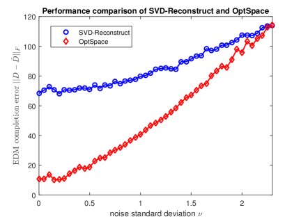
Figure 1 illustrates our results. We can see that when the standard deviation of noise is low (i.e., below $\nu=2.3$ approximately), the average completion error of SVD-Reconstruct is larger than that of OptSpace. The simulation result agrees with our theoretical analysis that SVD-Reconstruct is suboptimal under low noise levels.

Proof of Theorem 4.

The proof is divided into two steps. First, we reduce the estimation problem to a hypothesis testing problem. The point lies in that the minimax risk can be lower bounded by the probability of error in a hypothesis testing problem. Once this is done, we will use some well-established tools (e.g., Fano’s inequality) in information theory to establish a lower bound on the error probability of the testing problem, and obtain the lower bound for the minimax rate. Let us now give a detailed proof.
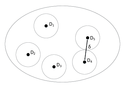
Step 1: From estimation to testing. In this step, we consider a finite subset $\mathcal{D}_{0}\subset\mathcal{D}(r)$ which is a $\delta$-packing of $\mathcal{D}(r)$. Here, $\delta$-packing means that for any two distinct matrix $\bm{D}_{u}$, $\bm{D}_{v}\in\mathcal{D}_{0}$,

$$\|\bm{D}_{u}-\bm{D}_{v}\|_{F}\geq\delta.$$

See Fig. 2 for an example. Given the $\delta$-packing set, we assume that the complete true matrix $\bm{D}$ in (2) is taken uniformly at random (u.a.r.) from $\mathcal{D}_{0}$.

Figure 2: Example of a $\delta$-packing of a set. Here, $\mathcal{D}_{0}=\{D_{1},D_{2},D_{3},D_{4},D_{5}\}$

Now with these setup, we obtain the following hypothesis testing problem: Given the observed matrix $\bm{Y}$, we need to determine which $\bm{D}_{u}\in\mathcal{D}_{0}$ is the groundtruth $\bm{D}$. Note that here we do not specify a test function $\Phi:\bm{Y}\rightarrow\bm{D}_{u}\in\mathcal{D}_{0}$. Lemma 16 gives us the relationship between minimax risk $\mathfrak{R}$ and the error probability $\mathbb{P}\{\Phi(\bm{Y})\neq\bm{D}\}$:

$$\mathfrak{R}\geq\frac{\delta}{2}\inf_{\Phi}\mathbb{P}\{\Phi(\bm{Y})\neq\bm{D}\},$$

where the infimum is taken over all testing functions. It remains to bound the error probability $\mathbb{P}\{\Phi(\bm{Y})\neq\bm{D}\}$. We will use Fano’s inequality to do this.
Step 2: Bound error probability. Fano’s inequality (Lemma 17 and 18) gives a lower bound for the error probability. But if we want to apply Lemma 18 in our zero-diagonal symmetric low-rank matrix completion model (2), we must consider the effect of $\bm{\Omega}$. Different from other estimation problems, here $\bm{\Omega}$ is random and unfixed. As a result, Lemma 18 cannot be applied directly unless we condition on $\bm{\Omega}$:

$$\mathbb{P}(\hat{\bm{D}}\neq\bm{D}|\bm{\Omega})\geq 1-\frac{I(\bm{D};\bm{Y}|\bm{\Omega})+\log 2}{\log|\mathcal{D}_{0}|}.$$

By the law of total probability and taking expectation with respect to $\bm{\Omega}$ on both sides of the above inequality, we get

$$\mathbb{P}(\hat{\bm{D}}\neq\bm{D})=\mathbb{E}_{\bm{\Omega}}\mathbb{P}(\hat{\bm{D}}\neq\bm{D}|\bm{\Omega})\geq 1-\frac{\mathbb{E}_{\bm{\Omega}}I(\bm{D};\bm{Y}|\bm{\Omega})+\log 2}{\log|\mathcal{D}_{0}|}.$$

Substituting this into Lemma 16, the minimax rate $\mathfrak{R}$ has the following lower bound:

$$\mathfrak{R}\geq\frac{\delta}{2}\Big{(}1-\frac{\mathbb{E}_{\bm{\Omega}}I(\bm{D};\bm{Y}|\bm{\Omega})+\log 2}{\log|\mathcal{D}_{0}|}\Big{)}.$$ (15)

Let us now discuss how to choose a suitable $\delta$. Intuitively, if we let $\delta\rightarrow 0$, the right-hand side of (15) becomes trivial, as it tends to be zero as well. Therefore, $\delta$ should be sufficiently large. In practice, a common approach is to choose the largest $\delta>0$ which makes the mutual information small enough, e.g.,

$$\frac{\mathbb{E}_{\bm{\Omega}}I(\bm{D};\bm{Y}|\bm{\Omega})+\log 2}{\log|\mathcal{V}|}\leq\frac{1}{2}.$$ (16)

In this case, the minimax risk is lower bounded by $\mathfrak{R}\geq\frac{\delta}{4}$.

In order to bound the left-hand side of (16), we need a lower bound for the cardinality of the $\delta$-packing set $\mathcal{D}_{0}$ and an upper bound for the mutual information $I(\bm{D};\bm{Y}|\bm{\Omega})$. For the cardinality of $\mathcal{D}_{0}$, Lemma 20 establishes the desired result:

$$|D_{0}|\geq\exp\big{(}\frac{rn}{128}\big{)}.$$

To establish an upper bound for the mutual information, a typical method involves the Kullback-Leibler divergence (KL-divergence). Before doing this, let us introduce some necessary notations first. Let $P_{\bm{Y}}$ denote the distribution of $\bm{Y}$ conditioned on $\bm{\Omega}$, $P_{u}$ denote the distribution of $\bm{Y}$ conditioned on $\bm{\Omega}$ and $\bm{D}=\bm{D}_{u}\in\mathcal{D}_{0}$, and $D_{KL}(f\|g)$ denote the KL-divergence of distribution $f$ and $g$. Then the mutual information can be bounded as follows:

$$I(\bm{D};\bm{Y}|\bm{\Omega}) =\frac{1}{|\mathcal{D}_{0}|}\sum_{u:\bm{D}_{u}\in\mathcal{D}_{0}}D_{KL}(P_{u}\|P_{\bm{Y}})$$

$$\leq\frac{1}{|\mathcal{D}_{0}|^{2}}\sum_{u,v:\bm{D}_{u}\in\mathcal{D}_{0},\bm{D}_{v}\in\mathcal{D}_{0}}D_{KL}(P_{u}\|P_{v}),$$

where the equality can be derived by a standard calculation, and the inequality is due to the convexity of the $-\log$ function. It remains to calculate the K-L divergence between $P_{u}$ and $P_{v}$. Conditioning on $\bm{\Omega}$, either $P_{u}$ or $P_{v}$ is a shifted version of the distribution of $\bm{\mathcal{E}}$. Here, we need to be careful, since the noise matrix $\bm{\mathcal{E}}$ is a symmetric matrix, which results in that some of the entries $\bm{\mathcal{E}}_{ij}$’s are dependent. An iterative application of Lemma 21 shows that the K-L divergence between $P_{u}$ and $P_{v}$ is totally determined by the independent part:

$$D_{KL}(P_{u}\|P_{v})=D_{KL}(P^{\prime}_{u}\|P^{\prime}_{v}),$$

where $P^{\prime}_{u}$ denotes the distribution of $\{\bm{Y}_{ij}:i\leq j\}$ conditioning on $\bm{\Omega}$ and $\bm{D}=\bm{D}_{u}$ and $P^{\prime}_{v}$ denotes the distribution of $\{\bm{Y}_{ij}:i\leq j\}$ conditioning on $\bm{\Omega}$ and $\bm{D}=\bm{D}_{v}$.

Since now both $P^{\prime}_{u}$ and $P^{\prime}_{v}$ are multivariate normal distributions with independent entries of different mean and same variance, the KL-divergence between them can be easily computed:

$$D_{KL}(P^{\prime}_{u}\|P^{\prime}_{v}) =\frac{1}{2\nu^{2}}\big{\|}\bm{\Omega}\odot\bm{D}_{u}\odot\bm{U}-\bm{\Omega}\odot\bm{D}_{v}\odot\bm{U}\big{\|}_{F}^{2}$$

$$\leq\frac{1}{2\nu^{2}}\big{\|}\bm{\Omega}\odot(\bm{D}_{u}-\bm{D}_{v})\big{\|}_{F}^{2},$$

where $\bm{U}$ is a matrix which takes value $1$ on or above the diagonal, and $0$ otherwise. Taking expectation to $\bm{\Omega}$ both sides, we get

$$\mathbb{E}_{\bm{\Omega}}D_{KL}(P_{u}\|P_{v}) \leq\frac{1}{2\nu^{2}}\mathbb{E}_{\bm{\Omega}}\big{\|}\bm{\Omega}\odot(\bm{D}_{u}-\bm{D}_{v})\big{\|}_{F}^{2}$$

$$=\frac{p}{2\nu^{2}}\big{\|}\bm{D}_{u}-\bm{D}_{v}\big{\|}_{F}^{2}.$$

Thus the minimax risk $\mathfrak{R}$ can be bounded by:

$$\mathfrak{R} \geq\frac{\delta}{2}\mathbb{P}\{\Phi(Y)\neq D\}\geq\frac{\delta}{2}\Big{(}1-\frac{\mathbb{E}_{\bm{\Omega}}I(\bm{D};\bm{Y}|\bm{\Omega})+\log 2}{\log|\mathcal{D}_{0}|}\Big{)}$$

$$\geq\frac{\delta}{2}\Bigg{[}1-\frac{\mathbb{E}_{\bm{\Omega}}\Big{(}\frac{1}{|\mathcal{D}_{0}|^{2}}\sum_{u,v}D(P_{u}\|P_{v})\Big{)}+\log 2}{\log|\mathcal{D}_{0}|}\Bigg{]}$$

$$=\frac{\delta}{2}\Bigg{[}1-\frac{\frac{1}{|\mathcal{D}_{0}|^{2}}\sum_{u,v}\mathbb{E}_{\bm{\Omega}}D(P_{u}\|P_{v})+\log 2}{\log|\mathcal{D}_{0}|}\Bigg{]}$$

$$=\frac{\delta}{2}\Bigg{[}1-\frac{\frac{p}{2\nu^{2}|\mathcal{D}_{0}|^{2}}\sum_{u,v}\|\bm{D}_{u}-\bm{D}_{v}\|_{F}^{2}+\log 2}{\log|\mathcal{D}_{0}|}\Bigg{]}.$$ (17)

Substituting Lemma 20 into (IV), we get

$$\mathfrak{R} \geq\frac{\delta}{2}\Bigg{[}1-\frac{\frac{p}{2\nu^{2}|\mathcal{D}_{0}|^{2}}|\mathcal{D}_{0}|^{2}\delta^{2}+\log 2}{\frac{rn}{128}}\Bigg{]}$$

$$\geq\frac{\delta}{2}\Bigg{[}1-\frac{\frac{64p\delta^{2}}{\nu^{2}}+128\log 2}{rn}\Bigg{]}.$$

Let $\frac{64p\delta^{2}}{\nu^{2}}=\frac{rn}{4}$, namely $\delta=\sqrt{\frac{rn\nu^{2}}{256p}}$, and assume that $rn\geq 512\log 2$, then

$$\mathfrak{R} \geq\frac{\delta}{2}\Bigg{[}1-\frac{\frac{64p\delta^{2}}{\nu^{2}}+128\log 2}{rn}\Bigg{]}$$

$$\geq\frac{1}{2}\sqrt{\frac{rn\nu^{2}}{256p}}\big{(}1-\frac{1}{4}-\frac{1}{4}\big{)}=\frac{\nu}{64}\sqrt{\frac{rn}{p}}=\frac{n\nu}{64}\sqrt{\frac{rn}{m}}.$$

This completes the proof. ∎

V Conclusion

In this paper, we have presented a detailed analysis for the SVD-MDS approach. We established error bounds for EDM completion by SVD-Reconstruct and for coordinate recovery by MDS using tools from random matrix theory. To investigate the optimality of SVD-Reconstruct, we derived the minimax lower bound for the zero-diagonal symmetric low-rank matrix completion problem. The result reveals that when the noise level is high, the SVD-Reconstruct approach can achieve the optimal minimax rate up to a constant factor; when the noise level is low, SVD-Reconstruct is minimax suboptimal, so it is sensible to develop (or employ) more effective methods to complete the EDM and hence localize the positions of nodes.

Appendix A Lemmas Used for Proof of Theorem 1

Lemma 1 (Symmetrization, [22], Lemma 6.3).

Let $F:\mathbb{R}_{+}\rightarrow\mathbb{R}$ be an increasing convex function. Assume that $\bm{X}_{1},\dots,\bm{X}_{N}$ are independent, mean zero random vectors in a normed space, and $\epsilon_{1},\dots,\epsilon_{N}$ are independent symmetric Bernoulli random variables. Then

$$\mathbb{E}F\Big{(}\frac{1}{2}\Big{\|}\sum_{i=1}^{N}\epsilon_{i}\bm{X}_{i}\Big{\|}\Big{)}\leq\mathbb{E}F\Big{(}\Big{\|}\sum_{i=1}^{N}\bm{X}_{i}\Big{\|}\Big{)}\leq\mathbb{E}F\Big{(}2\Big{\|}\sum_{i=1}^{N}\epsilon_{i}\bm{X}_{i}\Big{\|}\Big{)}.$$

Lemma 2 (Contraction principle, [22], Theorem 4.4).

Let $\bm{x}_{1},\dots,\bm{x}_{N}$ be (deterministic) vectors in a normed space, $\epsilon_{1},\dots,\epsilon_{N}$ be independent symmetric Bernoulli random variables, and let $\bm{a}=(a_{1},\dots,a_{n})\in\mathbb{R}^{n}$ be a coefficient vector. Then

$$\mathbb{E}\Big{\|}\sum_{i=1}^{N}a_{i}\epsilon_{i}\bm{x}_{i}\Big{\|}\leq\|a\|_{\infty}\cdot\mathbb{E}\Big{\|}\sum_{i=1}^{N}\epsilon_{i}\bm{x}_{i}\Big{\|}.$$

Lemma 3 (Seginer’s theorem, [23], Theorem 1.1).

There exists a constant $K$ such that, for any $m,n$ any $h\leq 2\log\max\{m,n\}$ and any $m\times n$ random matrix $\bm{A}=(a_{ij})$, where $a_{ij}$ are i.i.d. zero mean random variables, the following inequality holds:

$$\max\big{\{}\mathbb{E}\max_{1\leq i\leq m}\|\bm{a}_{i\cdot}\|^{h},\mathbb{E}\max_{1\leq j\leq n}\|\bm{a}_{\cdot j}\|^{h}\big{\}}\leq\mathbb{E}\|\bm{A}\|^{h}$$

$$\leq(2K)^{h}\big{(}\mathbb{E}\max_{1\leq i\leq m}\|\bm{a}_{i\cdot}\|^{h}+\mathbb{E}\max_{1\leq j\leq n}\|\bm{a}_{\cdot j}\|^{h}\big{)},$$

where $\bm{a}_{i\cdot}$ and $\bm{a}_{\cdot j}$ denote the $i$-th row and the $j$-th column of the matrix $\bm{A}$, respectively.

Lemma 4.

(1) Let $X\sim\textnormal{Bin}(n,p)$ and $X_{1},\dots,X_{n}$ be i.i.d. copies of $X$. Let $Z=\max_{i\leq n}X_{i}$. If $p\geq\ln n/n$, then

$$\mathbb{E}Z\leq Cnp,$$

where $C$ is an absolute constant.
(2) Let $\bm{W}$ be an $n\times n$ random matrix with i.i.d Bernoulli entries, i.e., $\mathbb{P}\{\bm{W}_{ij}=1\}=p$ and $\mathbb{P}\{\bm{W}_{ij}=0\}=1-p$, and let $\bm{G}$ denote an $n\times n$ random matrix whose entries are i.i.d standard Gaussian random variables. Then

$$E\max_{1\leq i\leq n}\|(\bm{W}\odot\bm{G})_{i\cdot}\|_{2}\leq c\sqrt{np},$$

where $c$ is an absolute constant.

Proof.

See Appendix B. ∎

Appendix B Proof of Lemma 4

To prove Lemma 4, we need the following facts:

Lemma 5 (Integral identity).

For any random variable $X$, we have

$$\mathbb{E}X=\int_{0}^{\infty}\mathbb{P}\{X>t\}dt-\int_{-\infty}^{0}\mathbb{P}\{X<t\}dt.$$

In particular, for a non-negative random variable $X$, we have

$$\mathbb{E}X=\int_{0}^{\infty}\mathbb{P}\{X>t\}dt.$$

Lemma 6 (Chernoff’s inequality, [24], Theorem 4.4).

Let $X_{i}$ be independent Bernoulli random variables with parameter $p_{i}$. Consider their sum $S_{N}=\sum_{i=1}^{N}X_{i}$ and denote its mean by $\mu=\mathbb{E}S_{N}$. Then, for any $t>\mu$, we have

$$\mathbb{P}\{S_{N}\geq t\}\leq e^{-\mu}\Big{(}\frac{e\mu}{t}\Big{)}^{t}.$$

In particular, for any $t\geq e^{2}\mu$ we have

$$\mathbb{P}\{S_{N}\geq t\}\leq e^{-t}.$$

Lemma 7 (Equivalence of sub-Gaussian properties, [25], Lemma 5.5).

Let $X$ be a random variable. Then the following properties are equivalent with parameters $K_{i}>0$ differing from each other by at most an absolute constant factor.

1. The tails of $X$ satisfy

$$\mathbb{P}\{|X|>t\}\leq\exp(1-t^{2}/K_{1}^{2})\textnormal{ for all }t\geq 0.$$

2. The moments of $X$ satisfy

$$\|X\|_{p}=(\mathbb{E}|X|^{p})^{1/p}\leq K_{2}\sqrt{p}.$$

3. The moment generating function (MGF) of $X$ satisfies

$$\mathbb{E}\exp(X^{2}/K_{3}^{2})\leq 2.$$

The sub-Gaussian random variable is defined through the above sub-Gaussian properties.

Definition 8 (Sub-Gaussian random variable, [25], Definition 5.7).

A random variable $X$ that satisfy one of the equivalent properties $1-3$ in Lemma 9 is called a sub-Gaussian random variable. The sub-Gaussian norm of $X$, denoted $\|X\|_{\psi_{2}}$ is defined to be the smallest $K_{3}$ in property $3$. In other words,

$$\|X\|_{\psi_{2}}=\inf\{t>0:\mathbb{E}\exp(X^{2}/t^{2})\leq 2\}.$$

Lemma 9 (Equivalence of sub-exponential properties, [25], pp. 221).

Let $X$ be a random variable. Then the following properties are equivalent with parameters $K_{i}>0$ differing from each other by at most an absolute constant factor.

1. The tails of $X$ satisfy

$$\mathbb{P}\{|X|>t\}\leq\exp(1-t/K_{1})\textnormal{ for all }t\geq 0.$$

2. The moments of $X$ satisfy

$$\|X\|_{p}=(\mathbb{E}|X|^{p})^{1/p}\leq K_{2}p.$$

3. The moment generating function (MGF) of $X$ satisfies

$$\mathbb{E}\exp(X/K_{3})\leq 2.$$

The sub-exponential random variable is defined through the above sub-exponential properties.

Definition 10 (Sub-exponential random variable, [25], Definition 5.13).

A random variable $X$ that satisfy one of the equivalent properties $1-3$ in Lemma 9 is called a sub-exponential random variable. The sub-exponential norm of $X$, denoted $\|X\|_{\psi_{1}}$ is defined to be the smallest $K_{3}$ in property $3$. In other words,

$$\|X\|_{\psi_{1}}=\inf\{t>0:\mathbb{E}\exp(X/t)\leq 2\}.$$

The sub-exponential random variables have the following two remarkable properties:

Lemma 11 (Centering, [25], Remark 5.18).

If $X$ is a sub-exponential random variable then $X-\mathbb{E}X$ is sub-exponential too, and

$$\|X-\mathbb{E}X\|_{\psi_{1}}\leq C\|X\|_{\psi_{1}},$$

where $C$ is an absolute constant.

Lemma 12 (Product of sub-Gaussian is sub-exponential, [26], Lemma 2.7.5).

Let $X$ and $Y$ be sub-Gaussian random variables. Then $XY$ is sub-exponential. Moreover,

$$\|XY\|_{\psi_{1}}\leq\|X\|_{\psi_{2}}\|Y\|_{\psi_{2}}.$$

Lemma 13 (Sub-exponential is sub-Gaussian squared, [25], Lemma 5.14).

A random variable $X$ is sub-Gaussian if and only if $X^{2}$ is sub-exponential. Moreover,

$$\|X^{2}\|_{\psi_{1}}\leq\|X\|^{2}_{\psi_{2}}.$$

In particular, if $g\sim N(0,\nu^{2})$, we have $g^{2}$ is sub-exponential, and

$$\|g^{2}\|_{\psi_{1}}\leq c\nu^{2}.$$

Lemma 14 (Bernstein-type inequality).

Let $X$ be a centered random variable satisfying

$$\mathbb{P}\big{\{}X\geq t\big{\}}\leq p\exp(-ct),$$

where $0<p<1$ and $c$ are constant numbers. Let $X_{1},\dots,X_{n}$ be independent copies of $X$. Then

$$\mathbb{P}\Big{\{}\sum_{i=1}^{n}X_{i}\geq t\Big{\}} \leq\exp\Big{[}-c\cdot\min\Big{(}\frac{t^{2}}{np},t\Big{)}\Big{]}$$

$$\leq\left\{\begin{array}[]{ll}\exp\big{(}-\dfrac{ct^{2}}{np}\big{)},&t\leq np,\\ \exp\big{(}-ct\big{)},&t>np.\end{array}\right.$$

Proof.

See Appendix G. ∎

Now we are ready to prove Lemma 4.
(1) By integral identity (Lemma 5), we know that

$$\mathbb{E}\max_{1\leq i\leq n}X_{i} =\int_{0}^{\infty}\mathbb{P}\{\max_{1\leq i\leq n}X_{i}>t\}dt$$

$$\leq\int_{0}^{s}1dt+\int_{s}^{\infty}\mathbb{P}\{\max_{1\leq i\leq n}X_{i}>t\}dt$$

$$=s+\int_{s}^{\infty}\mathbb{P}\{\bigcup\limits_{1\leq i\leq n}X_{i}>t\}dt$$

$$\leq s+\int_{s}^{\infty}\sum_{i=1}^{n}\mathbb{P}\{X_{i}>t\}dt$$

$$=s+\sum_{i=1}^{n}\int_{s}^{\infty}\mathbb{P}\{X_{i}>t\}dt.$$

If we let $s=e^{2}np$, by Chernoff’s inequality (Lemma 6), we have

$$\mathbb{E}\max_{1\leq i\leq n}X_{i} \leq s+\sum_{i=1}^{n}\int_{s}^{\infty}\mathbb{P}\{X_{i}>t\}dt$$

$$\leq e^{2}np+\sum_{i=1}^{n}\int_{e^{2}np}^{\infty}e^{-t}dt$$

$$=e^{2}np+ne^{-e^{2}np}.$$

Recall that we have assumed that $np\geq\log n$, thus

$$\mathbb{E}\max_{1\leq i\leq n}X_{i} \leq e^{2}np+ne^{-e^{2}np}$$

$$\leq e^{2}np+ne^{-e^{2}\log n}$$

$$=e^{2}np+n^{1-e^{2}}$$

$$\leq(e^{2}+1)np,$$

where the last inequality comes from the fact that $n^{-e^{2}}\leq n^{-1}\leq\frac{\ln n}{n}\leq p$. This completes the proof of the first part of Lemma 4.

(2) The proof of the second part is similar to that of the first part. First,

$$\mathbb{E}\max_{1\leq i\leq n}\|(\bm{W}\odot\bm{G})_{i\cdot}\|_{2}^{2}$$

$$\leq\mathbb{E}\max_{1\leq i\leq n}\sum_{j=1}^{n}\bm{W}_{ij}^{2}(\bm{G}_{ij}^{2}-1)+\mathbb{E}\max_{1\leq i\leq n}\sum_{j=1}^{n}\bm{W}_{ij}^{2}.$$

The second term can be bounded by part (1):

$$\mathbb{E}\max_{1\leq i\leq n}\sum_{j=1}^{n}\bm{W}_{ij}^{2}\leq c_{1}np.$$

For the first term, let $\bm{T}_{ij}=\bm{W}_{ij}^{2}(\bm{G}_{ij}^{2}-1)$, then for any $t>0$, we have

$$\mathbb{P}\big{\{}\bm{T}_{ij}\geq t\big{\}} =\mathbb{P}\big{\{}\bm{W}_{ij}^{2}(\bm{G}_{ij}^{2}-1)\geq t|\bm{W}_{ij}=1\big{\}}\mathbb{P}\{\bm{W}_{ij}=1\}$$

$$\hskip 11.1pt+\mathbb{P}\big{\{}\bm{W}_{ij}^{2}(\bm{G}_{ij}^{2}-1)\geq t|\bm{W}_{ij}=0\big{\}}\mathbb{P}\{\bm{W}_{ij}=0\}$$

$$=p\mathbb{P}\big{\{}\bm{G}_{ij}^{2}-1\geq t\big{\}}$$

$$\leq p\exp(-ct),$$ (18)

where the last inequality holds because $\bm{G}_{ij}^{2}-1=\bm{G}_{ij}^{2}-\mathbb{E}\bm{G}_{ij}^{2}$ is a sub-exponential random variable by Lemma 11 and 13, and $\|\bm{G}_{ij}^{2}-1\|_{\psi_{1}}\leq c^{\prime}\|\bm{G}_{ij}^{2}\|_{\psi_{1}}\leq c^{\prime}\|\bm{G}_{ij}\|_{\psi_{2}}^{2}\leq c^{\prime\prime}$, where $c^{\prime}$ and $c^{\prime\prime}$ are absolute constants. Thus, Lemma 14 can be used to bound the tail probability of $\sum_{j=1}^{n}\bm{T}_{ij}$:

$$\mathbb{P}\Big{\{}\sum_{j=1}^{n}\bm{T}_{ij}\geq t\Big{\}} \leq\exp\Big{[}-c\cdot\min\Big{(}\frac{t^{2}}{np},t\Big{)}\Big{]}$$

$$\leq\left\{\begin{array}[]{ll}\exp\big{(}-\dfrac{ct^{2}}{np}\big{)},&t\leq np,\\ \exp\big{(}-ct\big{)},&t>np.\end{array}\right.$$ (21)

Similarly, we will use integral identity (Lemma 5) to bound the first term:

$$\mathbb{E}\max_{1\leq i\leq n}\sum_{j=1}^{n}\bm{W}_{ij}^{2}(\bm{G}_{ij}^{2}-1)$$

$$=\int_{0}^{\infty}\mathbb{P}\big{\{}\max_{1\leq i\leq n}\sum_{j=1}^{n}\bm{W}_{ij}^{2}(\bm{G}_{ij}^{2}-1)\geq t\big{\}}dt$$

$$\leq\int_{0}^{np}1dt+n\int_{np}^{\infty}\mathbb{P}\big{\{}\sum_{j=1}^{n}\bm{W}_{ij}^{2}(\bm{G}_{ij}^{2}-1)\geq t\big{\}}dt$$

$$\leq np+n\int_{np}^{\infty}\exp\big{(}-ct\big{)}dt$$

$$\leq np+n\exp(-cnp)$$

$$\leq c_{2}np,$$

where the last inequality comes from the fact that $np\geq\log n$, and $c_{2}$ is an absolute constant. Combining the two terms, we get

$$\mathbb{E}\max_{1\leq i\leq n}\|(\bm{W}\odot\bm{G})_{i\cdot}\|_{2}^{2}\leq c_{3}np.$$

Then, Jensen’s inequality completes the proof:

$$\mathbb{E}\max_{1\leq i\leq n}\|(\bm{W}\odot\bm{G})_{i\cdot}\|_{2}\leq\big{[}\mathbb{E}\max_{1\leq i\leq n}\|(\bm{W}\odot\bm{G})_{i\cdot}\|_{2}^{2}\big{]}^{1/2}\leq c\sqrt{np}.$$

Appendix C Lemmas Used for Proof of Theorem 2

Lemma 15 (Matrix Bernstein inequality: sub-exponential case, [27], Lemma 6.2).

Consider a finite sequence ${\bm{X}_{k}}$ of independent, random, self-adjoint matrices with dimension $n$. Assume that each random matrix has zero mean, and satisfies

$$\mathbb{E}\bm{X}_{k}=0\ \ \textnormal{and}\ \ \mathbb{E}(\bm{X}_{k}^{p})\preceq\frac{p!}{2}\cdot R^{p-2}\cdot\bm{A}_{k}^{2}\ \textnormal{for }p=2,3,4\dots$$

Compute the variance parameter

$$\sigma^{2}:=\Big{\|}\sum_{k}\bm{A}_{k}^{2}\Big{\|}.$$

Then the following holds for all $t\geq 0$,

$$\mathbb{P}\Big{\{}\Big{\|}\sum_{k}\bm{Z}_{k}\Big{\|}\geq t\Big{\}}\leq n\cdot\exp\Big{[}-c\cdot\min\Big{(}\frac{t^{2}}{\sigma^{2}},\frac{t}{R}\Big{)}\Big{]},$$

where $c$ is an absolute constant.

Appendix D Lemmas Used for Proof of Theorem 4

Lemma 16 ([21], pp. 79-80).

For any test function $\Phi:\bm{Y}\rightarrow\bm{D}_{u}\in\mathcal{D}_{0}$, the minimax risk $\mathfrak{R}$ in (13) has the following lower bound:

$$\mathfrak{R}\geq\frac{\delta}{2}\mathbb{P}\{\Phi(\bm{Y})\neq\bm{D}\}.$$

Lemma 17 (Fano inequality, [28], Theorem 2.10.1).

Suppose $V$ is a random variable taking values in a finite set $\mathcal{V}$. For any Markov chain $V\rightarrow X\rightarrow\hat{V}$, we have

$$h_{2}\big{(}\mathbb{P}(\hat{V}\neq V)\big{)}+\mathbb{P}(\hat{V}\neq V)\log(|\mathcal{V}|-1)\geq H(V|\hat{V}),$$ (22)

where the function $h_{2}(p)=-p\log p-(1-p)\log(1-p)$ denotes the entropy of the Bernoulli random variable with parameter $p$, and $H(V|\hat{V})$ denotes the entropy of $V$ conditioned on $\hat{V}$.

Moreover, if we assume that $V$ takes value u.a.r. on $\mathcal{V}$, Lemma 17 becomes

Lemma 18.

Assume that $V$ is uniform on $\mathcal{V}$. For any Markov chain $V\rightarrow X\rightarrow\hat{V}$,

$$\mathbb{P}(\hat{V}\neq V)\geq 1-\frac{I(V;X)+\log 2}{\log|\mathcal{V}|},$$

where $I(V;X)$ denotes the mutual information of random variable $V$ and $X$.

Lemma 19 (Bounding the mutual information, [28]).

$$I(\bm{D};\bm{Y}|\bm{\Omega}) =\frac{1}{|\mathcal{D}_{0}|}\sum_{u:\bm{D}_{u}\in\mathcal{D}_{0}}D_{KL}(P_{u}\|P_{\bm{Y}})$$

$$\leq\frac{1}{|\mathcal{D}_{0}|^{2}}\sum_{u,v:\bm{D}_{u}\in\mathcal{D}_{0},\bm{D}_{v}\in\mathcal{D}_{0}}D_{KL}(P_{u}\|P_{v}).$$

The proof of Theorem 4 is based on the following lemma:

Lemma 20.

Let $n\geq 10$ be a positive integer, and let $\delta>0$. Then for each $r=2,\dots,n$, there exists a set of $n$-dimensional matrices $\{\bm{D}^{1},\bm{D}^{2},\dots,\bm{D}^{M}\}$ with cardinality $M=\lfloor\exp\big{(}\frac{rn}{128}\big{)}\rfloor$ such that each matrix is symmetric, with zero diagonal, has rank at most $r$, and moreover

$$\|\bm{D}^{l}\|_{F}=\delta\quad\text{for all }l=1,2,\dots,M,$$

$$\|\bm{D}^{k}-\bm{D}^{l}\|_{F}\geq\delta\quad\text{for all }k\neq l.$$

Proof.

See Appendix E. ∎

Lemma 21.

Let $p(x_{1},x_{2})$ denote the probability density function (p.d.f) of $X=(X_{1},X_{2})$, $q(x_{1},x_{2})$ denote the p.d.f of $X^{\prime}=(X^{\prime}_{1},X^{\prime}_{2})$, $p(x_{1})$ denote the p.d.f of $X_{1}$, and $q(x_{1})$ denote the p.d.f of $X^{\prime}_{1}$, where $X_{2}=X_{1}$, $X^{\prime}_{2}=X^{\prime}_{1}$. Then, the K-L divergence between $p(x_{1},x_{2})$ and $q(x_{1},x_{2})$ is equal to that of $p(x_{1})$ and $q(x_{1})$:

$$D_{KL}\big{(}p(x_{1},x_{2})\|q(x_{1},x_{2})\big{)}=D_{KL}\big{(}p(x_{1})\|q(x_{1})\big{)}.$$

Proof.

See Appendix F. ∎

Appendix E Proof of Lemma 20

The idea for proof of Lemma 20 is inspired by Negahban and Wainwright [29]. It relies on the Hoeffding’s inequality, which gives a tail bound for sum of independent Rademaker random variables.

Lemma 22 (Hoeffding’s inequality, [30], Theorem 2).

Let $X_{1}$,…,$X_{N}$ be independent symmetric Bernoulli random variables, and $\bm{a}=(a_{1},\dots,a_{N})\in\mathbb{R}^{N}$. Then, for any $t>0$, we have

$$\mathbb{P}\Big{\{}\sum_{i=1}^{N}a_{i}X_{i}\geq t\Big{\}}\leq\exp\Big{(}-\frac{t^{2}}{2\|\bm{a}\|_{2}^{2}}\Big{)}.$$

We proceed via the probabilistic method, in particular by showing that a random procedure succeeds in generating such a set with probability at least $0.22$. Let $M=\lfloor\exp\big{(}\frac{rn}{128}\big{)}\rfloor$, and for each $l=1,2,\dots,M$, we draw a random matrix $\bm{\tilde{D}}^{l}\in\mathbb{R}^{n\times n}$ according to the following procedure:

(a) For rows $i=1,\dots,\lfloor\frac{r}{2}\rfloor$ and columns $j=i+1,\dots,n$, choose each $\bm{\tilde{D}}^{l}_{ij}\in\{-1,+1\}$ uniformly at random, independently across $(i,j)$.

(b) For columns $j=1,\dots,\lfloor\frac{r}{2}\rfloor$ and rows $i=j+1,\dots,n$, set $\bm{\tilde{D}}^{l}_{ij}=\bm{\tilde{D}}^{l}_{ji}$.

(c) For rows $i=\lfloor\frac{r}{2}\rfloor+1,\dots,n$ and columns $j=\lfloor\frac{r}{2}\rfloor+1,\dots,n$, and for $1\leq i=j\leq n$, set $\bm{\tilde{D}}^{l}_{ij}=0$.

By construction, each matrix $\bm{\tilde{D}}^{l}$ is symmetric, with zero diagonal, and has rank at most $r$. Since there exists a ceil operator in $\frac{r}{2}$, we go ahead by considering $r$ is even and odd separately.
Case 1: $r$ is even and $r\geq 2$.
In this case $\lfloor\frac{r}{2}\rfloor=\frac{r}{2}$, and the Frobenius norm $\|\tilde{\bm{D}}^{l}\|_{F}=\sqrt{r(n-r/4-1/2)}$. We define $\bm{D}^{l}=\frac{\delta}{\sqrt{r(n-r/4-1/2)}}\bm{\tilde{D}}^{l}$ for all $l=1,\dots,M$. The rescaled matrices $\bm{D}^{l}$ has Frobenius norm $\|\bm{D}^{l}\|_{F}=\delta$. We now prove that

$$\|\bm{D}^{l}-\bm{D}^{k}\|_{F}\geq\delta\quad\text{for all }l\neq k$$

holds with probability at least $0.46$. Now to prove Lemma 20, it suffices to show that $\|\bm{\tilde{D}}^{l}-\bm{\tilde{D}}^{k}\|_{F}\geq\sqrt{r(d-r/4-1/2)}$ with probability at least $0.46$ for any pair $l\neq k$. We have

$$\frac{1}{r(n-r/4-1/2)}\|\bm{\tilde{D}}^{l}-\bm{\tilde{D}}^{k}\|_{F}^{2}$$

$$=\frac{2}{r(n-r/4-1/2)}\cdot\Big{[}\sum_{i=1}^{r/2}\sum_{j=i+1}^{n}(\bm{\tilde{D}}^{l}_{ij}-\bm{\tilde{D}}^{k}_{ij})^{2}\Big{]}.$$

This is a sum of i.i.d. variables, each taking value $\{0,4\}$ with equal probability, so the Hoeffding’s inequality (Lemma 22) implies that for any $t\geq 0$,

$$\mathbb{P}\Bigg{\{}\frac{2}{r(n-r/4-1/2)}\cdot$$

$$\hskip 57.0pt\bigg{\{}\sum_{i=1}^{r/2}\sum_{j=i+1}^{n}\Big{[}\frac{1}{2}(\bm{\tilde{D}}^{l}_{ij}-\bm{\tilde{D}}^{k}_{ij})^{2}-1\Big{]}\bigg{\}}\leq-t\Bigg{\}}$$

$$\leq\exp\Bigg{\{}-\frac{t^{2}}{2\cdot\sum\limits_{i=1}^{r/2}\sum\limits_{j=i+1}^{n}\big{(}\frac{2}{r(n-r/4-1/2)}\big{)}^{2}}\Bigg{\}}$$

$$\leq\exp\Big{[}-\frac{r(n-r/4-1/2)t^{2}}{4}\Big{]}.$$

Therefore,

$$\mathbb{P}\{\frac{1}{r(n-r/4-1/2)}\|\bm{\tilde{D}}^{l}-\bm{\tilde{D}}^{k}\|_{F}^{2}\leq 2-t\}$$

$$\leq\exp\Big{[}-\frac{r(n-r/4-1/2)t^{2}}{16}\Big{]}$$

$$\leq\exp\Big{(}-\frac{rnt^{2}}{32}\Big{)},$$

where in the last inequality we have used the fact that $n\geq r\geq 2$. Since there are less than $M^{2}$ pairs of matrices in total, by taking union bound we get

$$\mathbb{P}\{\min_{l\neq k}\frac{1}{r(n-r/4)}\|\bm{\tilde{D}}^{l}-\bm{\tilde{D}}^{k}\|_{F}^{2}\leq 2-t\}\leq M^{2}\exp\Big{(}-\frac{rnt^{2}}{32}\Big{)}.$$

Letting $t=1$ and substituting $M=\lfloor\exp\big{(}\frac{rn}{128}\big{)}\rfloor$, we get

$$\mathbb{P}\Big{\{}\min_{l\neq k}\frac{1}{r(n-r/4)}\|\bm{\tilde{D}}^{l}-\bm{\tilde{D}}^{k}\|_{F}^{2}\leq 1\Big{\}}$$

$$\leq\exp\Big{(}\frac{rn}{64}\Big{)}\exp\Big{(}-\frac{rn}{32}\Big{)}$$

$$=\exp\Big{(}-\frac{rn}{64}\Big{)}.$$

Namely,

$$\mathbb{P}\Big{\{}\min_{l\neq k}\|\bm{\tilde{D}}^{l}-\bm{\tilde{D}}^{k}\|_{F}^{2}\geq r(n-r/4)\Big{\}}$$

$$\geq 1-\exp\Big{[}-\frac{rn}{64}\Big{]}\geq 0.26,$$

where in the last inequality we have used the fact that $n\geq 10$ and $r\geq 2$.
Case 2: $r$ is odd and $r\geq 3$.
In the case of $r$ is odd, $\lfloor\frac{r}{2}\rfloor=\frac{r-1}{2}$, and the Frobenius norm $\|\tilde{\bm{D}}^{l}\|_{F}=\sqrt{(r-1)(n-(r-1)/4-1/2)}$. We define $\bm{D}^{l}=\frac{\delta}{\sqrt{(r-1)(n-(r-1)/4-1/2)}}\bm{\tilde{D}}^{l}$ for all $l=1,\dots,M$. Similarly as case 1, we will prove that the procedure generates a sequence of matrices satisfying

$$\|\bm{\tilde{D}}^{l}-\bm{\tilde{D}}^{k}\|_{F}\geq\sqrt{(r-1)(n-(r-1)/4-1/2)}$$

with probability at least $0.2$. We proceed the same as case 1, and obtain that

$$\mathbb{P}\{\min_{l\neq k}\frac{1}{(r-1)(n-(r-1)/4)}\|\bm{\tilde{D}}^{l}-\bm{\tilde{D}}^{k}\|_{F}^{2}\geq 1\}$$

$$\geq 1-\exp\Big{[}-\frac{5rn}{576}\Big{]}\geq 0.22,$$

where the last inequality holds because $n\geq 10$ and $r\geq 3$.

Combining these two cases and recalling the definition of $\bm{D}^{l}$ completes the proof.

Appendix F Proof of Lemma 21

To prove Lemma 21, we need the following two properties of K-L divergence:

Lemma 23 (information inequality, [28], Theorem 2.6.3).

Let $p(x),q(x)$ be two probability density functions. Then,

$$D_{KL}\big{(}p(x)\|q(x)\big{)}\geq 0$$

with equality if and only if $p(x)=q(x)$ for all $x$.

Lemma 24 (Chain rule for K-L divergence, [28], Theorem 2.5.3).

Let $p(x_{1},x_{2})$ and $q(x_{1},x_{2})$ be the joint p.d.f’s of $(X_{1},X_{2})$ and $(X^{\prime}_{1},X^{\prime}_{2})$, respectively. Denote $p(x_{1})$ and $q(x_{1})$ the marginal p.d.f’s of $X_{1}$ and $X^{\prime}_{1}$, and $p(x_{2}|x_{1})$ and $q(x_{2}|x_{1})$ the conditional p.d.f’s of $X_{2}$ conditioning on $X_{1}$ and $X^{\prime}_{2}$ conditioning on $X^{\prime}_{1}$, respectively. Then

$$D_{KL}\big{(}p(x_{1},x_{2})\|q(x_{1},x_{2})\big{)}\\ =D_{KL}\big{(}p(x_{1})\|q(x_{1})\big{)}+\mathbb{E}_{x_{1}}D_{KL}\big{(}p(x_{2}|x_{1})\|q(x_{2}|x_{1})\big{)}.$$

Proof of Lemma 21.

According to the chain rule for K-L divergence (Lemma 24), the K-L divergence between $p(x_{1},x_{2})$ and $q(x_{1},x_{2})$ can be written as

$$D_{KL}\big{(}p(x_{1},x_{2})\|q(x_{1},x_{2})\big{)}\\ =D_{KL}\big{(}p(x_{1})\|q(x_{1})\big{)}+\mathbb{E}_{x_{1}}D_{KL}\big{(}p(x_{2}|x_{1})\|q(x_{2}|x_{1})\big{)},$$ (23)

By Lemma 21, we always have $X_{2}=X_{1}$ and $X^{\prime}_{2}=X^{\prime}_{1}$. As a result, the conditional p.d.f’s $p(x_{2}|x_{1})$ and $q(x_{2}|x_{1})$ are equivalent, i.e., both of them are delta functions at $x_{1}$. Hence, the information inequality (Lemma 23) implies that $D_{KL}\big{(}p(x_{2}|x_{1})\|q(x_{2}|x_{1})\big{)}=0$. Substituting this into (23) completes the proof. ∎

Appendix G Proof of Lemma 14

Lemma 14 is a Bernstein-type inequality, and the proof technique is standard. First, we bound the $n$-moments of $X$:

$$\mathbb{E}|X|^{n} =\int_{0}^{\infty}\mathbb{P}\big{\{}|X|\geq t\big{\}}nt^{n-1}dt$$

$$\leq\int_{0}^{\infty}p\exp(-ct)nt^{n-1}dt$$

$$\leq c_{1}pn^{n}.$$

Then the moment generating function of $X$ can be bounded by

$$\mathbb{E}\exp(\lambda X) =1+|\lambda|\mathbb{E}X+\sum_{k=2}^{\infty}\frac{|\lambda|^{k}\mathbb{E}X^{k}}{k!}$$

$$\leq 1+\sum_{k=2}^{\infty}\frac{|\lambda|^{k}c_{1}pk^{k}}{k!}$$

$$\leq 1+c_{1}p\sum_{k=2}^{\infty}(e|\lambda|)^{k}$$

$$\leq 1+c_{2}p\lambda^{2}\quad(\text{when }|\lambda|\leq 1/2e)$$

$$\leq\exp(c_{2}p\lambda^{2}).$$

Now the tail probability of $X_{i}$ can be bounded by

$$\mathbb{P}\big{\{}\sum_{i=1}^{n}X_{i}\geq t\big{\}} =\mathbb{P}\big{\{}\exp\big{(}\lambda\sum_{i=1}^{n}X_{i}\big{)}\geq\exp(\lambda t)\big{\}}$$

$$\leq e^{-\lambda t}\prod_{i}\mathbb{E}\exp(\lambda X_{i}).$$

If $|\lambda|\leq 1/2e$, then we have

$$\mathbb{P}\big{\{}\sum_{i=1}^{n}X_{i}\geq t\big{\}}\leq\exp(-\lambda t+c_{2}np\lambda^{2}).$$

It remains to optimize over $\lambda>0$. Choosing $\lambda=\min(t/2c_{2}np,1/2e)$ yields the desired result.

References

- [1] P. Drineas, A. Javed, M. Magdon-Ismail, G. Pandurangant, R. Virrankoski, and A. Savvides, “Distance matrix reconstruction from incomplete distance information for sensor network localization,” in 2006 3rd Annual IEEE Communications Society on Sensor and Ad Hoc Communications and Networks, vol. 2, Sep. 2006, pp. 536–544.
- [2] N. Patwari, J. N. Ash, S. Kyperountas, A. O. Hero, R. L. Moses, and N. S. Correal, “Locating the nodes: Cooperative localization in wireless sensor networks,” IEEE Signal Process. Mag., vol. 22, no. 4, pp. 54–69, Jul. 2005.
- [3] T. F. Havel and K. Wüthrich, “An evaluation of the combined use of nuclear magnetic resonance and distance geometry for the determination of protein conformations in solution,” J. Mol. Biol., vol. 182, no. 2, pp. 281–294, Aug. 1985.
- [4] I. Dokmanić, R. Parhizkar, A. Walther, Y. M. Lu, and M. Vetterli, “Acoustic echoes reveal room shape,” Proc. Natl. Acad. Sci., vol. 110, no. 30, pp. 12 186–12 191, Jun. 2013.
- [5] K. Q. Weinberger and L. K. Saul, “Unsupervised learning of image manifolds by semidefinite programming,” Proc. IEEE Conf. on Computer Vision and Pattern Recognition, vol. 2, pp. II–988–II–995, 2004.
- [6] W. S. Torgeson, “Multidimensional scaling of similarity,” Psychometrika, vol. 30, no. 4, pp. 379–393, Dec. 1965.
- [7] J. C. Gower, “Properties of euclidean and non-euclidean distance matrices,” Linear Algebra Appl., vol. 67, pp. 81–97, Jun. 1985.
- [8] ——, “Euclidean distance geometry,” Math. Sci., vol. 7, no. 1, pp. 1–14, Jan. 1982.
- [9] R. Parhizkar, A. Karbasi, S. Oh, and M. Vetterli, “Calibration using matrix completion with application to ultrasound tomography,” IEEE Trans. Signal Process., vol. 61, no. 20, pp. 4923–4933, Oct. 2013.
- [10] R. H. Keshavan, A. Montanari, and S. Oh, “Matrix completion from noisy entries,” IEEE Trans. Inf. Theory, vol. 56, no. 6, pp. 2980–2998, Jun. 2010.
- [11] A. Y. Alfakih, A. Khandani, and H. Wolkowicz, “Solving euclidean distance matrix completion problems via semidefinite programming,” Comput. Optim. Appl., vol. 12, no. 1, pp. 13–30, Jan. 1999.
- [12] P. Biswas, T. Liang, K. Toh, Y. Ye, and T. Wang, “Semidefinite programming approaches for sensor network localization with noisy distance measurements,” IEEE Trans. Autom. Sci. Eng., vol. 3, no. 4, pp. 360–371, Oct. 2006.
- [13] A. Javanmard and A. Montanari, “Localization from incomplete noisy distance measurements,” Found. Comput. Math., vol. 13, no. 3, pp. 297–345, 2013.
- [14] C. Ding and H. Qi, “Convex optimization learning of faithful euclidean distance representations in nonlinear dimensionality reduction,” Mathematical Programming, vol. 164, no. 1, pp. 341–381, Jul. 2017.
- [15] J. B. Kruskal, “Nonmetric multidimensional scaling: A numerical method,” Psychometrika, vol. 29, no. 2, pp. 115–129, Jun. 1964.
- [16] Y. Takane, F. Young, and J. D. Leeuw, “Nonmetric individual differences multidimensional scaling: An alternating least squares method with optimal scaling features,” Psychometrika, vol. 42, no. 1, pp. 7–67, Mar. 1977.
- [17] R. Parhizkar, “Euclidean distance matrices: Properties, algorithms and applications,” Ph.D. dissertation, School of Computer and Communication Sciences, Ecole Polytechnique Federale de Lausanne, 2013.
- [18] R. Z. Khas’mi, “A lower bound on the risks of nonparametric estimates of densities in the uniform metric,” Theory Probab. Appl., vol. 23, no. 4, pp. 794–798, Dec. 1976.
- [19] Y. Plan, R. Vershynin, and E. Yudovina, “High-dimensional estimation with geometric constraints,” Information and Inference: A Journal of the IMA, vol. 6, no. 1, pp. 1–40, Sep. 2017.
- [20] S. Oh, A. Montanari, and A. Karbasi, “Sensor network localization from local connectivity: Performance analysis for the mds-map algorithm,” in Information Theory (ITW 2010, Cairo), 2010 IEEE Information Theory Workshop on, Jan. 2010, pp. 1–5.
- [21] A. B. Tsybakov, Introduction to Nonparametric Estimation. Springer, 2009.
- [22] M. Ledoux and M. Talagrand, Probability in Banach Spaces: isoperimetry and processes. Springer, 1991.
- [23] Y. Seginer, “The expected norm of random matrices,” Combinatorics, Probability & Computing, vol. 9, no. 2, pp. 149–166, Mar. 2000.
- [24] M. Michael and U. Eli, Probability and Computing: Randomized Algorithms and Probabilistic Analysis. Cambridge University Press, 2005.
- [25] R. Vershynin, “Introduction to the non-asymptotic analysis of random matrices,” in Compressed Sensing: Theory and Applications. Cambridge: Cambridge University Press, May 2012, pp. 210–268.
- [26] ——, High-Dimensional Probability: An Introduction with Applications in Data Science. Draft, 2016.
- [27] J. Tropp, “User-friendly tail bounds for sums of random matrices,” Found. Comput. Math., vol. 12, no. 4, pp. 389–434, Aug. 2012.
- [28] T. M. Cover and J. A. Thomas, Elements of information theory, 2nd ed. Wiley-Interscience, 2008.
- [29] S. Negahban and M. J. Wainwright, “Restricted strong convexity and weighted matrix completion: Optimal bounds with noise,” J. Mach. Learn. Res., vol. 13, pp. 1665–1697, May 2012.
- [30] W. Hoeffding, “Probability inequalities for sums of bounded random variables,” Journal of the American Statistical Association, vol. 58, no. 301, pp. 13–30, Mar. 1963.