Optimal-Time Dictionary-Compressed Indexes

Abstract

We describe the first self-indexes able to count and locate pattern occurrences in optimal time within a space bounded by the size of the most popular dictionary compressors. To achieve this result we combine several recent findings, including string attractors — new combinatorial objects encompassing most known compressibility measures for highly repetitive texts —, and grammars based on locally-consistent parsing.

More in detail, let $\gamma$ be the size of the smallest attractor for a text $T$ of length $n$. The measure $\gamma$ is an (asymptotic) lower bound to the size of dictionary compressors based on Lempel–Ziv, context-free grammars, and many others. The smallest known text representations in terms of attractors use space $O(\gamma\log(n/\gamma))$, and our lightest indexes work within the same asymptotic space. Let $\epsilon>0$ be a suitably small constant fixed at construction time, $m$ be the pattern length, and $occ$ be the number of its text occurrences. Our index counts pattern occurrences in $O(m+\log^{2+\epsilon}n)$ time, and locates them in $O(m+(occ+1)\log^{\epsilon}n)$ time. These times already outperform those of most dictionary-compressed indexes, while obtaining the least asymptotic space for any index searching within $O((m+occ)\,\textrm{polylog}\,n)$ time. Further, by increasing the space to $O(\gamma\log(n/\gamma)\log^{\epsilon}n)$, we reduce the locating time to the optimal $O(m+occ)$, and within $O(\gamma\log(n/\gamma)\log n)$ space we can also count in optimal $O(m)$ time. No dictionary-compressed index had obtained this time before. All our indexes can be constructed in $O(n)$ space and $O(n\log n)$ expected time.

As a byproduct of independent interest, we show how to build, in $O(n)$ expected time and without knowing the size $\gamma$ of the smallest attractor (which is NP-hard to find), a run-length context-free grammar of size $O(\gamma\log(n/\gamma))$ generating (only) $T$. As a result, our indexes can be built without knowing $\gamma$.

Kociumaka supported by ISF grants no. 824/17 and 1278/16 and by an ERC grant MPM under the EU’s Horizon 2020 Research and Innovation Programme (grant no. 683064). Navarro supported by Fondecyt grant 1-170048, Chile; Basal Funds FB0001, Conicyt, Chile. Prezza supported by the project MIUR-SIR CMACBioSeq (“Combinatorial methods for analysis and compression of biological sequences”) grant no. RBSI146R5L.

A preliminary version of this article appeared in Proc. LATIN’18 [Christiansen and Ettienne (2018)].

Author’s addresses: Anders Roy Christiansen, The Technical University of Denmark, Denmark, aroy@dtu.dk. Mikko Berggren Ettienne, The Technical University of Denmark, Denmark, miet@dtu.dk. Tomasz Kociumaka, Department of Computer Science, Bar-Ilan University, Ramat Gan, Israel and Institute of Informatics, University of Warsaw, Poland, kociumaka@mimuw.edu.pl. Gonzalo Navarro, CeBiB – Center for Biotechnology and Bioengineering, Chile and Department of Computer Science, University of Chile, Chile, gnavarro@dcc.uchile.cl. Nicola Prezza, Department of Computer Science, University of Pisa, Italy, nicola.prezza@di.unipi.it.

1 Introduction

The need to search for patterns in large string collections lies at the heart of many text retrieval, analysis, and mining tasks, and techniques to support it efficiently have been studied for decades: the suffix tree, which is the landmark solution, is over 40 years old [Weiner (1973), McCreight (1976)]. The recent explosion of data in digital form led the research since 2000 towards compressed self-indexes, which support text access and searches within compressed space [Navarro and Mäkinen (2007)]. This research, though very successful, is falling short to cope to a new wave of data that is flooding our storage and processing capacity with volumes of higher orders of magnitude that outpace Moore’s Law [Stephens et al. (2015)]. Interestingly enough, this massive increase in data size is often not accompanied with a proportional increase in the amount of information that data carries: much of the fastest-growing data is highly repetitive, for example thousands of genomes of the same species, versioned document and software repositories, periodic sky surveys, and so on. Dictionary compression of those datasets typically reduces their size by two orders of magnitude [Gagie et al. (2018)]. Unfortunately, previous self-indexes build on statistical compression, which is unable to capture repetitiveness [Kreft and Navarro (2013)]; therefore, a new generation of compressed self-indexes based on dictionary compression is emerging.

Examples of successful compressors from this family include (but are not limited to) the Lempel–Ziv factorization [Lempel and Ziv (1976)], of size $z$; context-free grammars [Kieffer and Yang (2000)] and run-length context-free grammars [Nishimoto et al. (2016)], of size $g$; bidirectional macro schemes [Storer and Szymanski (1982)], of size $b$; and collage systems [Kida et al. (2003)], of size $c$. Other compressors that are not dictionary-based but also perform well on repetitive text collections are the run-length Burrows–Wheeler transform [Burrows and Wheeler (1994)], of size $\rho$, and the CDAWG [Blumer et al. (1987)], of size $e$. A number of compressed self-indexes have been built on top of those compressors; GNP18 give a thorough review.

Recently, KP18 showed that all the above-mentioned repetitiveness measures (i.e., $z$, $g$, $b$, $c$, $\rho$, $e$) are never asymptotically smaller than the size $\gamma$ of a new combinatorial object called string attractor. This and subsequent works [Kempa and Prezza (2018), Navarro and Prezza (2019), Prezza (2019)] showed that efficient access and searches can be supported within $O(\gamma\log(n/\gamma))$ space. By the nature of this new repetitiveness measure, such data structures are universal, in the sense that they can be used on top of a wide set of dictionary-compressed representations of $T$.

Our results

In this article we obtain the best results on attractor-based indexes, including the first optimal-time search complexities within space bounded in terms of $\gamma$, $z$, $g$, $b$, or $c$. We combine and improve upon three recent results:

1. [Thm. 2]NP18 presented the first index that builds on an attractor of size $\gamma$ of a text $T[1..n]$. It uses $O(\gamma\log(n/\gamma))$ space and finds the $occ$ occurrences of a pattern $P[1..m]$ in time $O(m\log n+occ(\log\log(n/\gamma)+\log^{\epsilon}\gamma))$ for any constant $\epsilon>0$.

2. [Thm. 2(3)]CE18 presented an index that builds on the Lempel–Ziv parse of $T$, of $z\geq\gamma$ phrases, which uses $O(z\log(n/z))$ space and searches in time $O(m+\log^{\epsilon}(z\log(n/z))+occ(\log\log n+\log^{\epsilon}z))$.

3. [Thm. 5]Nav18 presented the first index that builds on the Lempel–Ziv parse of $T$ and counts the number of occurrences of $P$ in $T$ (i.e., computes $occ$) in time $O(m\log n+m\log^{2+\epsilon}z)$, using $O(z\log(n/z))$ space.

Our contributions are as follows:

1. We obtain, in space $O(\gamma\log(n/\gamma))$, an index that lists all the occurrences of $P$ in $T$ in time $O(m+\log^{\epsilon}\gamma+occ\log^{\epsilon}(\gamma\log(n/\gamma)))$, thereby obtaining the best space and improving the time from previous works [Christiansen and Ettienne (2018), Navarro and Prezza (2019)].

2. We obtain, in space $O(\gamma\log(n/\gamma))$, an index that counts the occurrences of $P$ in $T$ in time $O(m+\log^{2+\epsilon}(\gamma\log(n/\gamma)))$, which outperforms the previous result [Navarro (2019)] both in time and space.

3. Using more space, $O(\gamma\log(n/\gamma)\log^{\epsilon}n)$, we list the occurrences in optimal $O(m+occ)$ time, and within space $O(\gamma\log(n/\gamma)\log n)$, we count them in optimal $O(m)$ time.

We can build all our structures in $O(n\log n)$ expected time and $O(n)$ working space, without the need to know the size $\gamma$ of the smallest attractor.

Our first contribution uses the minimum known asymptotic space, $O(\gamma\log(n/\gamma))$, for any dictionary-compressed index searching in time $O((m+occ)\,\mathrm{polylog}\,n)$ [Gagie et al. (2018)]. Only recently [Navarro and Prezza (2019)], it has been shown that it is possible to search within this space. Indeed, our new index outperforms most dictionary-compressed indexes, with a few notable exceptions like gagie2014lz77, who use $O(z\log(n/z))$ space and $O(m\log m+occ\log\log n)$ search time (but, unlike us, assume a constant alphabet), and PhBiCPM17, who use $O(z\log(n/z)\log\log z)$ space and $O(m+occ\log\log n)$ search time without making any assumption on the alphabet size. Our second contribution lies on a less explored area, since the first index able to count efficiently within dictionary-bounded space is very recent [Navarro (2019)].

Our third contribution yields the first indexes with space bounded in terms of $\gamma$, $z$, $g$, $b$, or $c$, multiplied by any $O(\textrm{polylog}\,n)$, that searches in optimal time. Such optimal times have been obtained, instead, by using $O(\rho\log(n/\rho))$ space [Gagie et al. (2018)], or using $O(e)$ space [Belazzougui and Cunial (2017)]. Measures $\rho$ and $e$, however, are not related to dictionary compression and, more importantly, have no known useful upper bounds in terms of $\gamma$. Further, experiments [Belazzougui et al. (2015), Gagie et al. (2018)] show that they are usually considerably larger than $z$ on repetitive texts.

As a byproduct of independent interest, we show how to build a run-length context-free grammar (RLCFG) of size $O(\gamma\log(n/\gamma))$ generating (only) $T$, where $\gamma$ is the size of the smallest attractor, in $O(n)$ expected time and without the need to know the attractor. We use this result to show that our indexes do not need to know an attractor, nor its minimum possible size $\gamma$ (which is NP-hard to obtain [Kempa and Prezza (2018)]) in order to achieve their attractor-bounded results. This makes our results much more practical. Another byproduct is the generalization of our results to arbitrary CFGs and, especially, RLCFGs, yielding slower times in $O(g)$ space, which can potentially be $o(\gamma\log(n/\gamma))$.

Techniques

A key component of our result is the fact that one can build a locally-consistent and locally-balanced grammar generating (only) $T$ such that only a few splits of a pattern $P$ must be considered in order to capture all of its “primary” occurrences [Kärkkäinen and Ukkonen (1996)]. Previous parsings had obtained $O(\log m\log^{*}n)$ [Nishimoto et al. (2019)] and $O(\log n)$ [Gawrychowski et al. (2018)] splits, but now we build on a parsing by DBLP:journals/algorithmica/MehlhornSU97 to obtain $O(\log m)$ splits with a grammar of size $O(\gamma\log(n/\gamma))$.

Our first step is to define a variant of Mehlhorn et al.’s randomized parsing and prove, in Section 3, that it enjoys several locality properties we require later for indexing. In Section 4, we use the parsing to build a RLCFG with the local balancing and local consistency properties we need. We then show, in Section 5, that the size of this grammar is bounded by $O(\gamma\log(n/\gamma))$, by proving that new nonterminals appear only around attractor positions.

In that section, we also show that the grammar can be built without knowing the minimum size $\gamma$ of an attractor of $T$. This is important because, unlike $z$, which can be computed in $O(n)$ time, finding $\gamma$ is NP-hard [Kempa and Prezza (2018)]. For this sake we define a new measure of compressibility, $\delta\leq\gamma$, which can be computed in $O(n)$ time and can be used to bound the size of the grammar.

Section 6 describes our index. We show how to parse the pattern in linear time using the same text grammar, and how to do efficient substring extraction and Karp–Rabin fingerprinting from a RLCFG. Importantly, we prove that only $O(\log m)$ split points are necessary in our grammar. All these elements are needed to obtain time linear in $m$. We also build on existing techniques [Claude and Navarro (2012)] to obtain time linear in $occ$ for the “secondary” occurrences; the primary ones are found in a two-dimensional data structure and require more time. Finally, by using a larger two-dimensional structure and introducing new techniques to handle short patterns, we raise the space to $O(\gamma\log(n/\gamma)\log^{\epsilon}n)$ but obtain the first dictionary-compressed index using optimal $O(m+occ)$ time.

In Section 7 we use the fact that only $O(\log m)$ splits must be considered to reduce the counting time of Nav18, while making its space attractor-bounded as well. This requires handling the run-length rules of RLCFGs, which turns out to require new ideas exploiting string periodicities. Further, by handling short patterns separately and raising the space to $O(\gamma\log(n/\gamma)\log n)$, we obtain the first dictionary-compressed index that counts in optimal time, $O(m)$.

Along the article we obtain various results on accessing and indexing specific RLCFGs. We generalize them to arbitrary CFGs and RLCFGs in Appendix A.

An earlier version of this article appeared in Proc. LATIN’18 [Christiansen and Ettienne (2018)]. This article is an exhaustive rewrite where we significantly extend and improve upon the conference results. We use a slightly different grammar, which requires re-proving all the results, in particular correcting and completing many of the proofs in the conference paper. We have also reduced the space by building on attractors instead of Lempel–Ziv parsing, used better techniques to report secondary occurrences and handle short patterns, and ultimately obtained optimal locating time. All the results on counting are also new.

2 Basic Concepts

Strings and texts

A string is a sequence $S[1\mathinner{.\,.}\ell]=S[1]S[2]\cdots S[\ell]$ of symbols. The symbols belong to an alphabet $\Sigma$, which is a finite subset of the integers. The length of $S$ is written as $|S|=\ell$.

A string $Q$ is a substring of $S$ if $Q$ is empty or $Q=S[i]\cdots S[j]$ for some indices $1\leq i\leq j\leq\ell$. The occurrence of $Q$ at position $i$ of $S$ is a fragment of $S$ denoted $S[i\mathinner{.\,.}j]$. We then also say that $S[i\mathinner{.\,.}j]$ matches $Q$. We assume implicit casting of fragments to the underlying substrings so that $S[i\mathinner{.\,.}j]$ may also denote $S[i]\cdots S[j]$ in contexts requiring strings rather than fragments.

A suffix of $S$ is a fragment of the form $S[i\mathinner{.\,.}\ell]$, and a prefix is a fragment of the form $S[1\mathinner{.\,.}i]$. The juxtaposition of strings and/or symbols represents their concatenation, and the exponentiation denotes the iterated concatenation. The reverse of $S[1\mathinner{.\,.}\ell]$ is $S^{rev}=S[\ell]S[\ell-1]\cdots S[1]$.

We will index a string $T[1\mathinner{.\,.}n]$, called the text. We assume our text to be flanked by special symbols $T[1]=\#$ and $T[n]=\$$ that belong to $\Sigma$ but occur nowhere else in $T$. This, of course, does not change any of our asymptotic results, but it simplifies matters.

Karp–Rabin signatures

Karp–Rabin fingerprinting [Karp and Rabin (1987)] assigns to every string $S[1\mathinner{.\,.}\ell]$ a signature $\kappa(S)=(\sum_{i=1}^{\ell}S[i]\cdot c^{i-1})\bmod\mu$ for a suitable integers $c$ and a prime number $\mu$. It is possible to build a signature formed by a pair of functions $\langle\kappa_{1},\kappa_{2}\rangle$ guaranteeing no collisions between substrings of $T[1\mathinner{.\,.}n]$, in $O(n\log n)$ expected time [Bille et al. (2014)].

With high probability

The term with high probability (w.h.p.) means with probability at least $1-n^{-c}$ for an arbitrary constant parameter $c$, where $n$ is the input size (in our case, the length of the text).

Model of computation

We use the RAM model with word size $w=\Omega(\log n)$, allowing classic arithmetic and bit operations on words in constant time. Our logarithms are to the base $2$ by default.

3 Locally-Consistent Parsing

A string $S[1\mathinner{.\,.}n]$ can be parsed in a locally consistent way, meaning that equal substrings are largely parsed in the same form. We use a variant of the parsing of DBLP:journals/algorithmica/MehlhornSU97.

Let us define a run in a string as a maximal substring repeating one symbol. The parsing proceeds in two passes. First, it groups the runs into metasymbols, which are seen as single symbols. The resulting sequence is denoted $\hat{S}[1\mathinner{.\,.}\hat{n}]$. The following definition describes the process precisely and defines mappings between $S$ and $\hat{S}$.

Definition 3.1.

The string $\hat{S}[1\mathinner{.\,.}\hat{n}]$ is obtained from a string $S[1\mathinner{.\,.}n]$ by replacing every distinct run $a^{\ell}$ in $S$ by a special metasymbol $a^{\ell}$ so that two occurrences of the same run $a^{\ell}$ are replaced by the same metasymbol. The alphabet $\hat{\Sigma}$ of $\hat{S}$ consists of the metasymbols that represent runs in $S$, that is $\hat{\Sigma}=\{\textrm{\framebox{$a^{\ell}$}}:a^{\ell}\text{ is a run in }S\}$.

A position $S[i]$ that belongs to a run $a^{\ell}$ is mapped to the position $\hat{S}[\hat{i}]$ of the corresponding metasymbol $a^{\ell}$, denoted $\hat{i}=map(i)$. A position $\hat{S}[\hat{i}]$ is mapped back to the maximal range $imap(\hat{i})=[fimap(\hat{i})\mathinner{.\,.}limap(\hat{i})]$ of positions in $S$ that map to $\hat{i}$. That is, if $S[i\mathinner{.\,.}i+\ell-1]$ is a run in $S$ that maps to $\hat{i}$, then $fimap(\hat{i})=i$ and $limap(\hat{i})=i+\ell-1$.

The string $\hat{S}$ is then parsed into blocks. A bijective function $\pi:\Sigma\rightarrow[1\mathinner{.\,.}|\Sigma|]$ is chosen uniformly at random; we call it a permutation. We then extend $\pi$ to $\hat{\Sigma}$ so that $\pi(\textrm{\framebox{$a^{\ell}$}})=\pi(a)$, that is, the value on a metasymbol is inherited from the underlying symbol. Note that no two consecutive symbols in $\hat{S}$ have the same $\pi$ value. We then define local minima in $\hat{S}$, and these are used to parse $\hat{S}$ (and $S$) into blocks.

Definition 3.2.

Given a string $S$, its corresponding string $\hat{S}[1\mathinner{.\,.}\hat{n}]$, and a permutation $\pi$ on the alphabet of $S$, a local minimum of $\hat{S}$ is defined as any position $\hat{i}$ such that $1<\hat{i}<\hat{n}$ and $\pi(\hat{S}[\hat{i}-1])>\pi(\hat{S}[\hat{i}])<\pi(\hat{S}[\hat{i}+1])$.

Definition 3.3.

The parsing of $\hat{S}$ partitions it into a sequence of blocks. The blocks end at position $\hat{n}$ and at every local minimum. The parsing of $\hat{S}$ induces a parsing on $S$: If a block ends at $\hat{S}[\hat{i}]$, then a block ends at $S[limap(\hat{i})]$.

Note that, by definition, the first block starts at $S[1]$. When applied on texts $S[1\mathinner{.\,.}n]$, it will hold that $\hat{S}[1]=\#$ and $\hat{S}[\hat{n}]=\$$, so $\hat{S}$ will also be a text. Further, we will always force that $\pi(\$)=1$ and $\pi(\#)=2$, which guarantees that there cannot be local minima in $\hat{S}[1\mathinner{.\,.}2]$ nor in $\hat{S}[\hat{n}-1\mathinner{.\,.}\hat{n}]$. Together with the fact that there cannot be two consecutive local minima, this yields the following observation.

Observation 3.4

Every block in $S$ or $\hat{S}$ is formed by at least two consecutive elements (symbols or metasymbols, respectively).

Definition 3.5.

We say that a position $p<n$ of the parsed text $S$ is a block boundary if a block ends at position $p$. For every non-empty fragment $S[i\mathinner{.\,.}j]$ of $S$, we define

$$B(i,j)=\{p-i:i\leq p<j\text{ and $p$ is a block boundary}\}.$$

Moreover, for every integer $c\geq 0$, we define subsets $L(i,j,c)$ and $R(i,j,c)$ of $B(i,j)$ consisting of the $\min(c,|B(i,j)|)$ smallest and largest elements of $B(i,j)$, respectively.

Observe that any fragment $S[i\mathinner{.\,.}j]$ intersects a sequence of $1+|B(i,j)|$ blocks (the first and the last block might not be contained in the fragment). We are interested in locally contracting parsings, where this number of blocks is smaller than the fragment’s length by a constant factor.

Definition 3.6.

A parsing is locally contracting if there exist constants $\alpha$ and $\beta<1$ such that $|B(i,j)|\leq\alpha+\beta|S[i\mathinner{.\,.}j]|$ for every fragment $S[i\mathinner{.\,.}j]$ of $S$.

Lemma 3.7.

The parsing of $S$ from Definition 3.3 is locally contracting with $\alpha=0$ and $\beta=\frac{1}{2}$.

Proof 3.8.

By 3.4, adjacent positions in $S$ cannot both be block boundaries. Hence, $|B(i,j)|\leq\lceil\frac{j-i}{2}\rceil=\lfloor\frac{j-i+1}{2}\rfloor=\lfloor\frac{1}{2}|S[i\mathinner{.\,.}j]|\rfloor\leq\frac{1}{2}|S[i\mathinner{.\,.}j]|$.

We formally define locally consistent parsings as follows.

Definition 3.9.

A parsing is locally consistent if there exists a constant $c_{p}$ such that for every pair of matching fragments $S[i\mathinner{.\,.}j]=S[i^{\prime}\mathinner{.\,.}j^{\prime}]$ it holds that $B(i,j)\setminus B(i^{\prime},j^{\prime})\subseteq L(i,j,c_{p})\cup R(i,j,c_{p})$, that is $B(i,j)$ and $B(i^{\prime},j^{\prime})$ differ by at most $c_{p}$ smallest and $c_{p}$ largest elements.

Next, we prove local consistency of our parsing.

Lemma 3.10.

The parsing of $S$ from Definition 3.3 is locally consistent with $c_{p}=1$. More precisely, if $S[i\mathinner{.\,.}j]=S[i^{\prime}\mathinner{.\,.}j^{\prime}]$ are matching fragments of $S$, then

$$B(i,j)\setminus\{limap(map(i))-i\}=B(i^{\prime},j^{\prime})\setminus\{limap(map(i))-i\}.$$

Proof 3.11.

By definition, a block boundary is a position $q$ such that $q=limap(\hat{q})$ for a local minimum $\hat{S}[\hat{q}]$ in $\hat{S}$. Hence, a position $q$, with $1<q<n$, is a block boundary if and only if $\pi(S[q])<\pi(S[q+1])$ and $\pi(S[q])<\pi(S[r])$, where $r=fimap(map(q))-1$ is the rightmost position to left of $q$ with $S[r]\neq S[q]$.

Consider a position $p$, with $i<p<j$, and the corresponding position $p^{\prime}=p-i+i^{\prime}$. If $p>limap(map(i))$, then the positions $r=fimap(map(p))-1$ and $r^{\prime}=fimap(map(p^{\prime}))-1$ satisfy $r^{\prime}-i^{\prime}=r-i\geq 0$. Hence, $p$ is a block boundary if and only if $p^{\prime}$ is one. On the other hand, if $p<limap(map(i))$, then neither $p$ nor $p^{\prime}$ is a block boundary because $S[p]=S[p+1]$ and $S[p^{\prime}]=S[p^{\prime}+1]$.

Consequently, only the position $p=limap(map(i))$ is a block boundary not necessarily if and only if $p^{\prime}$ is one. That is, $B(i,j)\setminus\{limap(map(i))-i\}=B(i^{\prime},j^{\prime})\setminus\{limap(map(i))-i\}$. Moreover, since $limap(map(i))-i$ may only be the leftmost element of $B(i,j)$, this yields $B(i,j)\setminus B(i^{\prime},j^{\prime})\subseteq L(i,j,1)$, and therefore the parsing is locally consistent with $c_{p}=1$.

We conclude this section by defining block extensions and proving that they are sufficiently long to ensure that the block is preserved within the occurrences of its extension. This property will be use several times in subsequent sections.

Definition 3.12.

Let $S[i\mathinner{.\,.}j]$, with $1<i<j<n$, be a block in $S$. The extension of the block $S[i\mathinner{.\,.}j]$ is defined as $S[i^{e}\mathinner{.\,.}j^{e}]$, where $i^{e}=fimap(map(i-1))-1$ and $j^{e}=j+1$.

Note that the first and last blocks cannot be extended. For the remaining blocks $S[i\mathinner{.\,.}j]$, the definition is sound because $map(i-1)>1$ and $j<n$ since $map(i-1)$ and $map(j)$ are local minima of $S^{\prime}$. Further, note that the block extension spans only the last symbol of the metasymbol $\hat{S}[map(i^{e})]$ and the first of $\hat{S}[map(j^{e})]$.

Lemma 3.13.

Let $S[i^{e}\mathinner{.\,.}j^{e}]$ be the extension of a block $S[i\mathinner{.\,.}j]$. If $S[r^{\prime}\mathinner{.\,.}s^{\prime}]$ matches $S[i^{e}\mathinner{.\,.}j^{e}]$, then $S[r^{\prime}\mathinner{.\,.}s^{\prime}]$ contains the same block $S[r\mathinner{.\,.}s]=S[i\mathinner{.\,.}j]$, whose extension is precisely $S[r^{e}\mathinner{.\,.}s^{e}]=S[r^{\prime}\mathinner{.\,.}s^{\prime}]$. Furthermore, $r-r^{e}=i-i^{e}$ and $s^{e}-s=j^{e}-j$.

Proof 3.14.

Observe that $limap(map(i^{e}))=i^{e}$, so Lemma 3.10 yields $B(r^{\prime},s^{\prime})\setminus\{0\}=B(i^{e},j^{e})\setminus\{0\}$. Moreover, $map(i^{e})=map(i-1)-1$ and $map(j^{e})=map(j)+1$, so $B(i^{e},j^{e})=\{i-1-i^{e},j-i^{e}\}$ due to 3.4. Hence, $B(r^{\prime},s^{\prime})\setminus\{0\}=\{i-1-i^{e},j-i^{e}\}$, and therefore $S[r\mathinner{.\,.}s]$ is a block, where $r=i-i^{e}+r^{\prime}$ and $s=j-i^{e}+r^{\prime}$. Figure 1 gives an example.

To complete the proof, notice that $s^{e}=s+1=s^{\prime}$ and $r^{e}=limap(map(r-1))-1=r^{\prime}$ follows from the fact that $S[r^{\prime}\mathinner{.\,.}s^{\prime}]$ and $S[i^{e}\mathinner{.\,.}j^{e}]$ match.

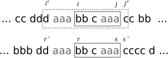
Figure 1: Illustration of Lemma 3.13. Local minima are shown in gray. Recall $r^{\prime}=r^{e}$ and $s^{\prime}=s^{e}$.

4 Grammars with Locality Properties

Consider a context-free grammar (CFG) that generates a string $S$ and only $S$ [Kieffer and Yang (2000)]. Each nonterminal must be the left-hand side in exactly one production, and the size $g$ of the grammar is the sum of the right-hand sides of the productions. It is NP-complete to compute the smallest grammar for a string $S$ [Rytter (2003), Charikar et al. (2005)], but it is possible to build grammars of size $g=O(z\log(|S|/z))$ if the Lempel–Ziv parsing of $S$ consists of $z$ phrases [Gawrychowski (2011), Lemma 8].

If we allow, in addition, rules of the form $A\rightarrow A_{1}^{s}$, where $s\geq 2$, taken to be of size 2 for technical convenience, the result is a run-length context-free grammar (RLCFG) [Nishimoto et al. (2016)]. These grammars encompass CFGs and are intrinsically more powerful; for example, the smallest CFG for the string family $S=a^{n}$ is of size $\Theta(\log n)$ whereas already an RLCFG of size $O(1)$ can generate it.

The parse tree of a CFG has internal nodes labeled with nonterminals and leaves labeled with terminals. The root is the initial symbol and the concatenation of the leaves yields $S$: the $i$th leaf is labeled $S[i]$. If $A\rightarrow A_{1}\cdots A_{s}$, then any node labeled $A$ has $s$ children, labeled $A_{1},\ldots,A_{s}$. In the parse tree of a RLCFG, rules $A\rightarrow A_{1}^{s}$ are represented as a node labeled $A$ with $s$ children nodes labeled $A_{1}$. The following definition describes the substring of $S$ generated by each node.

Definition 4.1.

If the leaves descending from a parse tree node $v$ are the $i$th to the $j$th leaves, we say that $v$ generates $S[i\mathinner{.\,.}j]$ and that $v$ is projected to the interval $proj(v)=[i\mathinner{.\,.}j]$.

The subtrees of equally labeled nodes are identical and generate the same strings, so we speak of the strings generated by the grammar symbols. We call $\exp(A)$ the expansion of nonterminal $A$, that is, the string it generates (or the concatenation of the leaves under any node labeled $A$ in the parse tree), and $|A|=|\exp(A)|$. For terminals $a$, we assume $\exp(a)=a$.

A grammar is said to be balanced if the parse tree is of height $O(\log n)$. A stricter concept is the following one.

Definition 4.2.

A grammar is locally balanced if there exists a constant $b$ such that, for any nonterminal $A$, the height of any parse tree node labeled $A$ is at most $b\cdot\log|A|$.

4.1 From parsings to balanced grammars

We build an RLCFG on a text $T[1\mathinner{.\,.}n]$ using our parsing of Section 3. In the first pass, we collect the distinct runs $a^{\ell}$ with $\ell\geq 2$ and create run-length nonterminals of the form $A\rightarrow a^{\ell}$ to replace the corresponding runs in $T$. The resulting sequence is analogous to $\hat{T}$, where a nonterminal $A\to a^{\ell}$ stands for the metasymbol $a^{\ell}$, and the terminal $a$ stands for the metasymbol $a^{1}$.

Next, we choose a permutation $\pi$ and perform a pass on the new text $\hat{T}$, defining the blocks based on local minima according to Definition 3.3. Each distinct block $A_{1}\cdots A_{k}$ is replaced by a distinct nonterminal $A$ with the rule $A\rightarrow A_{1}\cdots A_{k}$ (each $A_{i}$ can be a symbol of $\Sigma$ or a run-length nonterminal created in the first pass). The blocks are then replaced by those created nonterminals $A$, which results in a string $T^{\prime}$. The string $T^{\prime}$ is of length $n^{\prime}\leq\lfloor n/2\rfloor$, by Observation 3.4. Note that the first and last symbols of $T^{\prime}$ expand to blocks that contain # and $, respectively, and thus they are unique too. We can then regard $T^{\prime}$ as a text, by having its first nonterminal, $T^{\prime}[1]$, play the role of #, and the last, $T^{\prime}[n^{\prime}]$, play the role of $.

The process is then repeated again on $T^{\prime}$, and iterated for $h\leq\lfloor\log n\rfloor$ rounds, until a single nonterminal is obtained. This is the initial symbol of the grammar. We denote by $T_{r}[1\mathinner{.\,.}n_{r}]$ the text created in round $r$, so $T_{0}=T$ and $T_{1}=T^{\prime}$. We also denote by $\hat{T}_{r}[1\mathinner{.\,.}\hat{n}_{r}]$ the intermediate text obtained by collapsing runs in $T_{r}$. Figure 2 exemplifies the grammars we build and the corresponding parse tree.

Permutations

Grammar

$$\pi(\mathsf{\$_{3}}) =1$$

$$\pi(\mathsf{\#_{3}}) =2$$

$$\pi(\mathsf{\$_{2}}) =1$$

$$\pi(\mathsf{\#_{2}}) =2$$

$$\pi(\mathsf{E}) =3$$

$$\pi(\mathsf{D}) =4$$

$$\pi(\mathsf{\$_{1}}) =1$$

$$\pi(\mathsf{\#_{1}}) =2$$

$$\pi(\mathsf{A}) =3$$

$$\pi(\mathsf{C}) =4$$

$$\pi(\mathsf{B}) =5$$

$$\pi(\mathsf{\$}) =1$$

$$\pi(\mathsf{\#}) =2$$

$$\pi(\mathsf{d}) =3$$

$$\pi(\mathsf{c}) =4$$

$$\pi(\mathsf{b}) =5$$

$$\pi(\mathsf{a}) =6$$

$$\mathsf{S} \to\mathsf{\#_{3}\$_{3}}$$

$$\mathsf{\$_{3}} \to\mathsf{DD\$_{2}}$$

$$\mathsf{\#_{3}} \to\mathsf{\#_{2}DDE}$$

$$\mathsf{\$_{2}} \to\mathsf{B\$_{1}}$$

$$\mathsf{\#_{2}} \to\mathsf{\#_{1}BAA}$$

$$\mathsf{E} \to\mathsf{BBAA}$$

$$\mathsf{D} \to\mathsf{BC}$$

$$\mathsf{\$_{1}} \to\mathsf{c\$}$$

$$\mathsf{\#_{1}} \to\mathsf{\#ad}$$

$$\mathsf{A} \to\mathsf{aac}$$

$$\mathsf{C} \to\mathsf{aabc}$$

$$\mathsf{B} \to\mathsf{bd}$$

Parse tree

Figure 2: An example of the construction of our grammar. The top-left part shows the permutations $\pi$ assigned in each level, and the top-right part gives the complete grammar built (for simplicity we omit run-length nonterminals). The parse tree, shown on the bottom, also omits run-length nonterminals. The texts $T_{r}$ correspond to the subsequent levels of the parse tree (starting from the bottom). Level-$r$ block boundaries that are not run boundaries are depicted using dotted lines. For example, $T_{2}=\mathsf{\#_{2}DDEDD\$_{2}}$, $n_{2}=7$, and the level-2 block boundaries are $11,17,23,33,39,45$. On the other hand, $\hat{n}_{2}=5$ and the level-2 run boundaries are $11,23,33,45$. The corresponding parsings $\mathcal{P}_{2}$ and $\hat{\mathcal{P}}_{2}$ decompose $T$ as $\mathsf{\#adbdaacaac|bdaabc|bdaabc|bdbdaacaac|bdaabc|bdaabc|bdc\$}$ and $\mathsf{\#adbdaacaac|bdaabcbdaabc|bdbdaacaac|bdaabcbdaabc|bdc\$}$, respectively.

The height of the grammar is at most $2h\leq 2\lfloor\log n\rfloor$, because we create run-length rules and then block-rules in each round. This grammar is then balanced because, by Observation 3.4, $n_{r}\leq n/2^{r}$. Moreover, the grammar is locally balanced.

Lemma 4.3.

The grammar we build from our parsing is locally balanced with $b=2$.

Proof 4.4.

Because of Observation 3.4, any subtree rooted at a nonterminal $A$ in the parse tree (at least) doubles the number of nodes per round towards the leaves. If $A$ is formed in round $r$, then the subtree has height at most $2r$, and the expansion satisfies $|A|\geq 2^{r}$. The height of the subtree rooted at $A$ is thus at most $2r\leq 2\log|A|$.

4.2 Local consistency properties

We now formalize the concept of local consistency for our grammars. For each $r\in[0\mathinner{.\,.}h]$, the subsequent characters of $T_{r}$ naturally correspond to nodes of the parse tree of $T$, and the fragments $T[i\mathinner{.\,.}j]$ generated by these nodes form a decomposition of $T$. We denote this parsing of $T$ by $\mathcal{P}_{r}$. In other words, $T[i\mathinner{.\,.}j]$ is a block of $\mathcal{P}_{r}$ if and only if $[i\mathinner{.\,.}j]=proj(v)$ for some node $v$ labeled by a symbol in $T_{r}$. We refer to the blocks and block boundaries in this parsing as level-$r$ blocks and level-$r$ block boundaries. Analogously, we define a parsing $\hat{\mathcal{P}}_{r}$ with blocks corresponding to subsequent symbols of $\hat{T}_{r}$, and we refer to the underlying blocks and block boundaries as level-$r$ runs and level-$r$ run boundaries; see Figure 2.

Note that every level-$r$ run boundary is also a level-$r$ block boundary, and every level-$(r+1)$ block boundary is also a level-$r$ run boundary. Moreover, by 3.4 at most one out of every two subsequent level-$r$ run boundaries can be a level-$(r+1)$ block boundary.

Definition 4.5.

For every non-empty fragment $T[i\mathinner{.\,.}j]$ of $T$, the sets defined according to Definition 3.5 for the parsing $\mathcal{P}_{r}$ are denoted $B_{r}(i,j)$, $L_{r}(i,j,c)$, and $R_{r}(i,j,c)$. Analogously, we denote by $\hat{B}_{r}(i,j)$, $\hat{L}_{r}(i,j,c)$, and $\hat{R}_{r}(i,j,c)$ the sets defined for the parsing $\hat{\mathcal{P}}_{r}$.

These notions let us reformulate Lemma 3.10 so that it is directly applicable at every level $r$.

Lemma 4.6.

If matching fragments $T[i\mathinner{.\,.}j]$ and $T[i^{\prime}\mathinner{.\,.}j^{\prime}]$ both consist of full level-$r$ blocks, then the corresponding fragments of $T_{r}$ also match, so $B_{r}(i,j)=B_{r}(i^{\prime},j^{\prime})$ and $\hat{B}_{r}(i,j)=\hat{B}_{r}(i^{\prime},j^{\prime})$. Moreover, $B_{r+1}(i,j)\setminus\{\min\hat{B}_{r}(i,j)\}=B_{r+1}(i^{\prime},j^{\prime})\setminus\{\min\hat{B}_{r}(i,j)\}$ if $\hat{B}_{r}(i,j)\neq\emptyset$, and $B_{r+1}(i,j)=B_{r+1}(i^{\prime},j^{\prime})=\emptyset$ otherwise.

Proof 4.7.

We proceed by induction on $r$. The first two claims hold trivially for $r=0$: the fragments $T[i\mathinner{.\,.}j]$ and $T[i^{\prime}\mathinner{.\,.}j^{\prime}]$ of $T_{0}=T$ clearly match, and $B_{0}(i,j)=[0\mathinner{.\,.}j-i-1]=B_{0}(i^{\prime},j^{\prime})$. For $r>0$, on the other hand, $T[i\mathinner{.\,.}j]$ and $T[i^{\prime}\mathinner{.\,.}j^{\prime}]$ consist of full level-$(r-1)$ blocks, so the inductive assumption yields that the corresponding fragments of $T_{r-1}$ also match and that $B_{r}(i,j)=B_{r}(i^{\prime},j^{\prime})=\emptyset$ or $B_{r}(i,j)\setminus\{\min\hat{B}_{r-1}(i,j)\}=B_{r}(i^{\prime},j^{\prime})\setminus\{\min\hat{B}_{r-1}(i,j)\}$. In the latter case, we observe that $i-1$ and $i+\min\hat{B}_{r-1}(i,j)$ are subsequent level-$(r-1)$ run boundaries while $i-1$ is a level-$r$ block boundary, or $i=1$ and $i+\min\hat{B}_{r-1}(i,j)$ is the leftmost level-$(r-1)$ run boundary. Either way, $i+\min\hat{B}_{r-1}(i,j)$ cannot be a level-$r$ block boundary due to 3.4, so $B_{r}(i,j)\setminus\{\min\hat{B}_{r-1}(i,j)\}=B_{r}(i,j)$. A symmetric argument proves that $B_{r}(i^{\prime},j^{\prime})\setminus\{\min\hat{B}_{r-1}(i,j)\}=B_{r}(i^{\prime},j^{\prime})$, which lets conclude that $B_{r}(i,j)=B_{r}(i^{\prime},j^{\prime})$. Hence, the matching fragments of $T_{r-1}$ corresponding to $T[i\mathinner{.\,.}j]$ and $T[i^{\prime}\mathinner{.\,.}j^{\prime}]$ are parsed into the same blocks so the corresponding fragments of $T_{r}$ also match.

To prove the other two claims for arbitrary $r\geq 0$, notice that the fragments of $T_{r}$ corresponding to $T[i\mathinner{.\,.}j]$ and $T[i^{\prime}\mathinner{.\,.}j^{\prime}]$ are occurrences of the same string, denoted $P_{r}$. Hence, $\hat{B}_{r}(i,j)$ and $\hat{B}_{r}(i^{\prime},j^{\prime})$ are equal as they both correspond to the run boundaries in $P_{r}$. If $P_{r}$ consists of a single run (i.e., if $\hat{B}_{r}(i,j)=\emptyset$), then clearly $B_{r+1}(i,j)=B_{r+1}(i^{\prime},j^{\prime})=\emptyset$. Otherwise, Lemma 3.10 implies $B_{r+1}(i,j)\setminus\{\min\hat{B}_{r}(i,j)\}=B_{r+1}(i^{\prime},j^{\prime})\setminus\{\min\hat{B}_{r}(i,j)\}$.

Nevertheless, we define local consistency of a grammar as a stronger property than the one expressed in Lemma 4.6: we require that $B_{r}(i,j)$ and $B_{r}(i^{\prime},j^{\prime})$ resemble each other even if the matching fragments $T[i\mathinner{.\,.}j]$ and $T[i^{\prime}\mathinner{.\,.}j^{\prime}]$ do not consist of full blocks.

Definition 4.8.

The grammar we build is locally consistent if there is a constant $c_{g}$ such that the parsings $\mathcal{P}_{r}$ are all locally consistent with constant $c_{g}$.

In the rest of this section, we prove that our grammar is locally consistent with constant $c_{g}=3$. Our main tool is the following construction of sets $B_{r}(P)$ and $\hat{B}_{r}(P)$, consisting of the positions (relative to $P$) of context-insensitive level-$r$ block and run boundaries that are common to all occurrences of $P$ in $T$. Despite these sets are defined based on an occurrence of $P$ in $T$, we show in Lemma 4.12 that they do not depend on the choice of the occurrence.

Definition 4.9.

Let $P$ be a substring of $T$ and let $T[i\mathinner{.\,.}j]$ be its arbitrary occurrence in $T$. The sets $B_{r}(P)$ and $\hat{B}_{r}(P)$ for $r\geq 0$ are defined recursively, with $X+\delta=\{x+\delta:x\in X\}$.

$$B_{r}(P)=\left\{\!\begin{aligned} &[0\mathinner{.\,.}|P|-2]&&\text{if }r=0,\\ &B_{r}(i+1+\min\hat{B}_{r-1}(P),i+\max B_{r-1}(P))+1+\min\hat{B}_{r-1}(P)&&\text{if }\hat{B}_{r-1}(P)\neq\emptyset,\\ &\emptyset&&\text{if }\hat{B}_{r-1}(P)=\emptyset;\end{aligned}\right.$$

$$\hat{B}_{r}(P)=\left\{\begin{aligned} &\hat{B}_{r}(i+1+\min B_{r}(P),i+\max B_{r}(P))+1+\min B_{r}(P)&&\text{if }B_{r}(P)\neq\emptyset,\\ &\emptyset&&\text{if }B_{r}(P)=\emptyset.\end{aligned}\right.$$

Our index also relies on aset $M(P)$ designed as a superset of $B_{r}(i,j)\setminus B_{r}(P)$ for every $r$ and every occurrence $T[i\mathinner{.\,.}j]$ of $P$. In other words, $M(P)$ contains, for each $r$, positions within $P$ that may be level-$r$ block boundaries in some but not necessarily all occurrences of $P$.

Definition 4.10.

For a substring $P$ of $T$, the set $M(P)$ is defined to contain $\min B_{r}(P)$ and $\max B_{r}(P)$ for every $r\geq 0$ with $B_{r}(P)\neq\emptyset$, and $\min\hat{B}_{r}(P)$ for every $r\geq 0$ with $\hat{B}_{r}(P)\neq\emptyset$.

Example 4.11.

Consider $P=\mathsf{dbdaacaacbdaabcbdaabcbd}$ with occurrences $T[3\mathinner{.\,.}25]$ and $T[25\mathinner{.\,.}47]$ in text of Figure 2. For $r=0$, we define $B_{0}(P)=[0\mathinner{.\,.}21]$ and set $\hat{B}_{0}(P)=\{1,2,4,5,7,8,9,10,12,13,14,15,16,18,19,20\}=1+\hat{B}_{0}(4,24)=1+\hat{B}_{0}(26,46)$. For $r=1$, we set $B_{1}(P)=\{2,5,8,10,14,16,20\}=2+B_{1}(5,24)=2+B_{1}(27,46)$ and $\hat{B}_{1}(P)=\{8,10,14,16\}=3+\hat{B}_{1}(6,23)=3+\hat{B}_{1}(28,45)$. For $r=2$, we set $B_{2}(P)=\{14\}=9+B_{2}(12,19)=9+B_{2}(34,41)$ and $\hat{B}_{2}(P)=\emptyset=15+\hat{B}_{2}(18,17)=15+\hat{B}_{2}(40,39)$. For $r\geq 3$, we have $B_{r}(P)=\hat{B}_{r}(P)=\emptyset$. Consequently, $M(P)=\{0,1,2,8,14,20,21\}$.

We now show $B_{r}(P)$ contains all the level-$r$ block boundaries in any occurrence of $P$ in $T$ except possibly the first 3 and the last one, but those missing boundaries belong to $M(P)$.

Lemma 4.12.

For every substring $P$ of $T$ and every $r\geq 0$, the sets $B_{r}(P)$ and $\hat{B}_{r}(P)$ do not depend on the choice of an occurrence $T[i\mathinner{.\,.}j]$ of $P$. Moreover,

$$B_{r}(P)\cup L_{r}(i,j,3)\cup R_{r}(i,j,1)=B_{r}(i,j)\subseteq B_{r}(P)\cup M(P).$$ (1)

Proof 4.13.

We proceed by induction on $r$, proving the independence of $\hat{B}_{r}(P)$ only at step $r+1$. In the base case, $B_{0}(P)=[0\mathinner{.\,.}|P|-2]$ does not depend on the choice of the occurrence, and Eq. (1) is satisfied because $B_{0}(P)=B_{0}(i,j)$.

For the inductive step, we assume the claims hold for $B_{r}(P)$. If $B_{r}(P)=\emptyset$, then $\hat{B}_{r}(P)=B_{r+1}(P)=\emptyset$ do not depend on the occurrence of $P$. The inductive assumption yields $B_{r+1}(i,j)\subseteq B_{r}(i,j)\subseteq M(P)=B_{r+1}(P)\cup M(P)$ and $|B_{r+1}(i,j)|\leq|B_{r}(i,j)|=|L_{r}(i,j,3)\cup R_{r}(i,j,1)|\leq 4$, so $L_{r+1}(i,j,3)\cup R_{r+1}(i,j,1)=B_{r+1}(i,j)$ and Eq. (1) is satisfied.

We henceforth assume that $B_{r}(P)\neq\emptyset$. Since $B_{r}(P)\subseteq B_{r}(i,j)$, both $i+\min B_{r}(P)$ and $i+\max B_{r}(P)$ are level-$r$ block boundaries, and therefore $T[i+\min B_{r}(P)+1\mathinner{.\,.}i+\max B_{r}(P)]$ consists of full level-$r$ blocks. We conclude from Lemma 4.6 that $\hat{B}_{r}(P)$, as defined in Definition 4.9, does not depend on the occurrence of $P$. Moreover, the only position between $i+\min B_{r}(P)$ and $i+\max B_{r}(P)$ that may or may not be a level-$(r+1)$ block boundary depending on the context of $T[i\mathinner{.\,.}j]$ is $i+\min\hat{B}_{r}(P)$ provided that $\hat{B}_{r}(P)\neq\emptyset$. In particular, $B_{r+1}(P)$, as defined in Definition 4.9, also does not depend on the occurrence of $P$.

To prove that $B_{r+1}(P)$ satisfies Eq. (1), we consider two cases. First, suppose that $\hat{B}_{r}(P)=\emptyset$, that is, there are no level-$r$ run boundaries between $i+\min B_{r}(P)$ and $i+\max B_{r}(P)$. Since $\hat{B}_{r}(i,j)\subseteq B_{r}(i,j)$, the inductive assumption $B_{r}(i,j)=B_{r}(P)\cup L_{r}(i,j,3)\cup R_{r}(i,j,1)$ implies $\hat{B}_{r}(i,j)\subseteq\{\min B_{r}(P),\max B_{r}(P)\}\cup L_{r}(i,j,3)\cup R_{r}(i,j,1)$, while $B_{r}(i,j)\subseteq B_{r}(P)\cup M(P)$ yields $\hat{B}_{r}(i,j)\subseteq\{\min B_{r}(P),\max B_{r}(P)\}\cup M(P)=M(P)$, where the equality follows from Definition 4.10. The former assertions yields $|\hat{B}_{r}(i,j)|\leq 6$, and since $B_{r+1}(i,j)\subseteq\hat{B}_{r}(i,j)$ cannot contain two consecutive elements of $\hat{B}_{r}(i,j)$ by 3.4, we conclude that $|B_{r+1}(i,j)|\leq 3$. In particular, since $B_{r+1}(P)=\emptyset$ according to Definition 4.9, we have $B_{r+1}(P)\cup L_{r+1}(i,j,3)\cup R_{r+1}(i,j,1)=B_{r+1}(i,j)\subseteq B_{r+1}(P)\cup M(P)$ as claimed.

Next, suppose that $\hat{B}_{r}(P)\neq\emptyset$. Definition 4.9 clearly implies $B_{r+1}(P)\subseteq B_{r+1}(i,j)$, so it remains to prove that $B_{r+1}(i,j)$ is a subset of both $B_{r+1}(P)\cup L_{r+1}(i,j,3)\cup R_{r+1}(i,j,1)$ and $B_{r+1}(P)\cup M(P)$. We take $q\in B_{r+1}(i,j)$ and consider three cases.

1. [(1)]

2. If $q\leq\min\hat{B}_{r}(P)$, then $q\in(L_{r}(i,j,3)\cap M(P))\cup\{\min B_{r}(P),\min\hat{B}_{r}(P)\}$ and therefore $q\in\hat{L}_{r}(i,j,5)$. Since $B_{r+1}(i,j)$ cannot contain two consecutive elements of $\hat{B}_{r}(i,j)$ due to 3.4, $q\in B_{r+1}(i,j)\cap\hat{L}_{r}(i,j,5)$ implies $q\in L_{r+1}(i,j,3)$. Finally, $q\in M(P)\cup\{\min B_{r}(P),\min\hat{B}_{r}(P)\}=M(P)$, where the equality holds due to Definition 4.10.

3. If $q\geq\max B_{r}(P)$, then $q\in(R_{r}(i,j,1)\cap M(P))\cup\{\max B_{r}(P)\}$ and therefore $q\in\hat{R}_{r}(i,j,2)$. Since $B_{r+1}(i,j)$ cannot contain two consecutive elements of $\hat{B}_{r}(i,j)$ due to 3.4, $q\in B_{r+1}(i,j)\cap R_{r}(i,j,2)$ implies $q\in R_{r+1}(i,j,1)$. Finally, $q\in M(P)\cup\{\max B_{r}(P)\}=M(P)$, where the equality holds due to Definition 4.10.

4. If $\min\hat{B}_{r}(P)<q<\max B_{r}(P)$, then $q+i$ is a level-$(r+1)$ block boundary and $q\in B_{r+1}(P)$ by Definition 4.9.∎

Lemma 4.12 implies that the grammar constructed in this section is locally consistent with $c_{g}=3$. We conclude this section with a further characterization of the set $M(P)$.

Lemma 4.14.

For each substring $P=T[i\mathinner{.\,.}j]$, the set $M(P)$ satisfies the following properties:

1. [(a)]

2. If $B_{r}(i,j)\neq\emptyset$ for some $r\geq 0$, then $\min B_{r}(i,j)\in M(P)$,

3. If $\hat{B}_{r}(i,j)\neq\emptyset$ for some $r\geq 0$, then $\min\hat{B}_{r}(i,j)\in M(P)$,

4. $|M(P)|\leq 3\lceil\log|P|\rceil$.

Proof 4.15.

To prove (1) for any $r$, note that $B_{r}(P)\subseteq B_{r}(i,j)\subseteq B_{r}(P)\cup M(P)$ by Lemma 4.12. If $\min B_{r}(i,j)\notin B_{r}(P)$, then it belongs to $M(P)$. Otherwise, it must be equal to $\min B_{r}(P)$, which is in $M(P)$ by Definition 4.10.

The proof of (2) is similar: Since $\hat{B}_{r}(i,j)\subseteq B_{r}(i,j)$, either $\min\hat{B}_{r}(i,j)\in B_{r}(i,j)\setminus B_{r}(P)\subseteq M(P)$, or $\min\hat{B}_{r}(i,j)\in B_{r}(P)$. If $\min\hat{B}_{r}(i,j)\in\{\min B_{r}(P),\max B_{r}(P)\}$, then it is in $M(P)$ by Definition 4.10. Otherwise, $\min B_{r}(P)<\min\hat{B}_{r}(i,j)<\max B_{r}(P)$ and, by the choice of $\hat{B}_{r}(P)$ in Definition 4.9, $\min\hat{B}_{r}(i,j)=\min\hat{B}_{r}(P)$ is also in $M(P)$ by Definition 4.10.

To prove (3), notice that $|B_{r}(P)|\leq\frac{1}{2}|B_{r-1}(P)|$ holds for all $r$ due to Definition 4.9, 3.4, and $\min B_{r-1}(P)\notin B_{r}(P)$. This implies $|B_{r}(P)|\leq|B_{0}(P)|\cdot 2^{-r}<|P|\cdot 2^{-r}$, and therefore $\hat{B}_{r}(P)=B_{r}(P)=\emptyset$ for $r\geq\log|P|$. Definition 4.10 now yields the claim.

5 Bounding our Grammar in terms of Attractors

Let us first define the concept of attractors in a string [Kempa and Prezza (2018)].

Definition 5.1 ([Kempa and Prezza (2018)]).

An attractor of a string $S$ a set $\Gamma\subseteq[1\mathinner{.\,.}n]$ of positions in $S$ such that each non-empty substring $Q$ of $S$ has an occurrence $S[i\mathinner{.\,.}j]$ containing an attractor position, i.e., satisfying $i\leq p\leq j$ for some $p\in\Gamma$.

In this section, we show that the RLCFG of Section 4 is of size $g=O(\gamma\log(n/\gamma))$, where $\gamma$ is the minimum size of an attractor of $T$. The key is to prove that distinct nonterminals are formed only around the attractor elements. For this, we first prove that $T^{\prime}[1\mathinner{.\,.}n^{\prime}]$, where the blocks of $T$ are converted into nonterminals, contains an attractor of size at most $3\gamma$.

Lemma 5.2.

Let $\Gamma$ be an attractor of $T$, and let $\Gamma^{\prime}=\bigcup_{p\in\Gamma}[p^{\prime}-1\mathinner{.\,.}p^{\prime}+1]$, where $p^{\prime}$ is the position in $T^{\prime}$ of the nonterminal that covers $p$ in $T$. Then $\Gamma^{\prime}$ is an attractor of $T^{\prime}$.

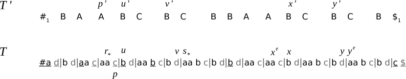
Figure 3: Illustration of Lemma 5.2. We underlined positions in $T$ corresponding to a particular string attractor.

Proof 5.3.

Figure 3 illustrates the proof. Consider an arbitrary substring $T^{\prime}[x^{\prime}\mathinner{.\,.}y^{\prime}]$, with $x^{\prime}\geq 3$ and $y^{\prime}\leq n^{\prime}-2$; otherwise the substring crosses an attractor because $1$ and $n$ are in $\Gamma$. This is a sequence of consecutive nonterminals, each corresponding to a block in $T$. Let $T[x\mathinner{.\,.}y]$ be the substring of $T$ formed by all the blocks that map to $T^{\prime}[x^{\prime}\mathinner{.\,.}y^{\prime}]$. The union of their extensions is also a substring $T[x^{e}\mathinner{.\,.}y^{e}]$ of $T$. Since $\Gamma$ is an attractor in $T$, there exists a copy $T[r_{*}\mathinner{.\,.}s_{*}]=T[x^{e}\mathinner{.\,.}y^{e}]$ that includes an element $p\in\Gamma$, $r_{*}\leq p\leq s_{*}$.

Consider any block $T[i\mathinner{.\,.}j]$ inside $T[x\mathinner{.\,.}y]$. Its extension $T[i^{e}\mathinner{.\,.}j^{e}]$ is contained in $T[x^{e}\mathinner{.\,.}y^{e}]$, so a copy $T[r^{\prime}\mathinner{.\,.}s^{\prime}]$ of $T[i^{e}\mathinner{.\,.}j^{e}]$ appears inside $T[r_{*}\mathinner{.\,.}s_{*}]$. By Lemma 3.13, the block $T[i\mathinner{.\,.}j]$ also forms a block $T[r\mathinner{.\,.}s]$ inside $T[r^{\prime}\mathinner{.\,.}s^{\prime}]$, at the same relative position; furthermore, $T[r^{\prime}\mathinner{.\,.}s^{\prime}]=T[r^{e}\mathinner{.\,.}s^{e}]$ is the extension of $T[r\mathinner{.\,.}s]$.

Since this happens for every block $T[i\mathinner{.\,.}j]$ inside $T[x\mathinner{.\,.}y]$, which is a sequence of blocks, it follows that $T[x\mathinner{.\,.}y]$ appears inside $T[r_{*}\mathinner{.\,.}s_{*}]$, as a subsequence $T[u\mathinner{.\,.}v]$ of blocks; furthermore, its extension $T[u^{e}\mathinner{.\,.}v^{e}]$ coincides with $T[r_{*}\mathinner{.\,.}s_{*}]$ and thus contains $p$. Moreover, $T[u\mathinner{.\,.}v]$ maps to a substring $T^{\prime}[u^{\prime}\mathinner{.\,.}v^{\prime}]=T^{\prime}[x^{\prime}\mathinner{.\,.}y^{\prime}]$.

Since $v^{e}=v+1$ and $u^{e}=fimap(map(u-1))-1$, due to Observation 3.4, the fragments $T[u^{e}\mathinner{.\,.}u-1]$ and $T[v+1\mathinner{.\,.}v^{e}]$ are contained within single blocks. Therefore, the position $p^{\prime}$ to which $p$ is mapped in $T^{\prime}$ belongs to $T^{\prime}[u^{\prime}-1\mathinner{.\,.}v^{\prime}+1]$. Consequently, $T^{\prime}[u^{\prime}\mathinner{.\,.}v^{\prime}]$ contains a position in $\Gamma^{\prime}$.

We now show that the first round contributes $O(\gamma)$ to the size of the final RLCFG. In this bound, we only count the the sizes of the generated rules; the whole accounting will be done in Theorem 5.6. The idea is to show that the $3$ distinct blocks formed around each attractor element have expected length $O(1)$.

Lemma 5.4.

The first round of parsing contributes $O(\gamma)$ to the grammar size, in expectation. Further, a parsing producing a grammar of size $O(\gamma)$ is found in $O(n)$ expected time provided that $\gamma$ is known.

Proof 5.5.

Let us first focus on block-forming rules; we consider the run-length rules in the next paragraph. The right-hand sides of the block-forming rules correspond to the distinct blocks formed in $\hat{T}$, that is, to single symbols in $T^{\prime}$. All the distinct symbols in $T^{\prime}$, in turn, appear at positions of $\Gamma^{\prime}$. By Lemma 5.2, $\Gamma^{\prime}$ is of size at most $3\gamma$; therefore, there are at most $3\gamma$ distinct blocks in $\hat{T}$ and in $T$ (i.e., those containing attractor elements of $T$ and their neighboring blocks), and thus at most $3\gamma$ distinct nonterminals are formed in the grammar.

We must also show, however, that the sum of the sizes of the right-hand sides of those $3\gamma$ productions also add up to $O(\gamma)$. Consider a block of $\hat{T}$ of length $\ell$. The right-hand side of its corresponding production is $\ell$. Each element of $\hat{T}$ can be a metasymbol, however, so the grammar may indeed include $\ell$ further run-length nonterminals, contributing up to $2\ell$ to the grammar size. Therefore, each distinct block of length $\ell$ in $\hat{T}$ contributes at most $3\ell$ to the grammar size. We now show that $\ell=O(1)$ in expectation for the $3\gamma$ blocks specified above.

Consider an attractor element $p$ and its position $\hat{p}=map(p)$ when mapped to $\hat{T}$. Let $T[i\mathinner{.\,.}j]$ be the block containing $p$ and let $T[i^{\prime}..j^{\prime}]$ be its concatenation with the adjacent blocks ($T[i^{\prime}\mathinner{.\,.}i-1]$ and $T[j+1\mathinner{.\,.}j^{\prime}]$). Moreover, let $\hat{T}[\hat{i}\mathinner{.\,.}\hat{j}]$ and $\hat{T}[\hat{i}^{\prime}\mathinner{.\,.}\hat{j}^{\prime}]$ be the corresponding fragments of $\hat{T}$, with $\hat{i}=map(i)$, $\hat{j}=map(j)$, $\hat{i}^{\prime}=map(i^{\prime})$, and $\hat{j}^{\prime}=map(j)$.

Let $\ell^{+}=\hat{j}^{\prime}-\hat{p}+1$, $\ell^{-}=\hat{p}-\hat{i}^{\prime}$, and $\ell=\ell^{+}+\ell^{-}$. Then, $3\ell$ is the maximum possible contribution of attractor $p$ to the grammar size via nonterminals that represent these blocks.

The area $\hat{T}[\hat{p}\mathinner{.\,.}\hat{j}^{\prime}]$ contains at most 2 local minima, at $\hat{j}$ and $\hat{j}^{\prime}$ (unless $\hat{j}^{\prime}=\hat{n}$). Note that, between two consecutive local minima, we have a sequence of nondecreasing values of $\pi$ and then a sequence of nonincreasing values of $\pi$. Our area can be covered by 2 such ranges. Hence, if we split the substring of length $\ell^{+}$ into 4 equal parts of length $\ell^{+}/4$, at least one of them must be monotone (i.e., nondecreasing or nonincreasing) with respect to $\pi$.

Note that consecutive symbols in $\hat{T}$ are always different. Further, if there are repeated symbols in a length-$d$ substring of $\hat{T}$, then it cannot be monotone with respect to $\pi$. If all the symbols are different, instead, exactly one out of $d!$ permutations $\pi$ will make the substring increasing and one out of $d!$ will make it decreasing, where $d$ is the length of the substring.

As a result, at most 2 out of $(\ell^{+}/4)!$ permutations can make one of our length-$(\ell^{+}/4)$ substrings monotone. If we choose permutations $\pi$ uniformly at random, then the probability that at least one of our 4 substrings is monotone is at most $8/(\ell^{+}/4)!$. Since this upper-bounds the probability that $\hat{j}^{\prime}\geq\hat{p}+\ell^{+}$, the expected value of $\ell^{+}$ is $O(1)$.

An analogous argument holds for $\ell^{-}$ since $\hat{T}[\hat{i}^{\prime}\mathinner{.\,.}\hat{p}-1]$ can also be covered by at most 2 ranges between consecutive local minima. Adding the expectations of the contributions $3\ell$ over the $\gamma$ attractor elements, we obtain $O(\gamma)$.

If the expectation is of the form $c\cdot\gamma$, then at least half of the permutations produce a grammar of size at most $2c\cdot\gamma$, and thus a Las Vegas algorithm finds a permutation producing a grammar of size at most $2c\cdot\gamma$ after $O(1)$ attempts in expectation. Since at each attempt we parse $T[1\mathinner{.\,.}n]$ in time $O(n)$, we find a suitable permutation in $O(n)$ expected time provided we know $\gamma$.

We now perform $O(\log(n/\gamma))$ rounds of locally-consistent parsing, where the output $T^{\prime}$ of each round is the input to the next. The length of the string halves in each iteration, and the grammar grows only by $O(\gamma)$ in each round.

Theorem 5.6.

Let $T[1\mathinner{.\,.}n]$ have an attractor of size $\gamma$. Then there exists a locally-balanced locally-consistent RLCFG of size $g=O(\gamma\log(n/\gamma))$ and height $O(\log(n/\gamma))$ that generates (only) $T$, and it can be built in $O(n)$ expected time and $O(g)$ working space if $\gamma$ is known.

Proof 5.7.

We apply the grammar construction described in Section 4.1, which by Lemmas 4.3 and 4.12, is locally balanced and locally consistent.

We first show that we can build an attractor $\Gamma_{r}$ for each $T_{r}$ formed by $\gamma$ runs of $m_{r}\in O(1)$ consecutive positions. This is clearly true for $T_{0}$, with $m_{0}=1$. Now assume this holds for $T_{r}$. When parsing $T_{r}$ into blocks to form $T_{r+1}$, each run of $m_{r}$ consecutive attractor positions is parsed into at most $1+\lfloor m_{r}/2\rfloor$ consecutive symbols $p^{\prime}$ in $T_{r+1}$, as seen in the proof of Lemma 3.7. Lemma 5.2 then shows that, if we expand each such mapped attractor positions $p^{\prime}$ to $[p^{\prime}-1\mathinner{.\,.}p^{\prime}+1]$, we obtain an attractor $\Gamma_{r+1}$ for $T_{r+1}$. The union of the expansions of $1+\lfloor m_{r}/2\rfloor$ consecutive positions $p^{\prime}$ creates a run of length $m_{r+1}=3+\lfloor m_{r}/2\rfloor$. It then holds that $\Gamma_{r+1}$ is formed by $\gamma$ runs of at most $m_{r+1}$ positions.

The sequence of values $m_{r}$ stabilizes. If we solve $m=3+\lfloor m/2\rfloor$, we obtain $\lceil m/2\rceil=3$. This solves for $m=5$ or $m=6$. Indeed, the value is 5 and is reached soon: $m_{0}=1$, $m_{1}=3$, $m_{2}=4$, $m_{3}=5$, $m_{4}=5$. Therefore, we safely use $m_{r}\leq 5$ in the following.

The only distinct blocks in each $T_{r}$ are those forming $\Gamma_{r+1}$. Therefore, the parsing of each text $T_{r}$ produces at most $5\gamma$ distinct nonterminal symbols. By Lemma 5.4, we can find in $O(n_{r})$ expected time a permutation $\pi_{r}$ such that the contribution of the $r$th round to the grammar size is $O(|\Gamma_{r}|)=O(\gamma)$.

The sum of the lengths of all $T_{r}$s is at most $2n$, thus the total expected construction cost is $O(n)$. We stop after $r^{*}=\log(n/\gamma)$ rounds. By then, $T_{r^{*}}$ is of length at most $\gamma$ and the cumulative size of the grammar is $O(\gamma\cdot r^{*})=O(\gamma\log(n/\gamma))$. We add a final rule $S\rightarrow T_{r^{*}}$, which adds $\gamma$ to the grammar size. The height of the grammar is $O(r^{*})=O(\log(n/\gamma))$.

As for the working space, at each new round $r$ we generate a permutation $\pi_{r}$ of $|\Sigma_{r}|$ cells. Since the alphabet size is a lower bound to the attractor size, it holds that $|\Sigma_{r}|\leq 5\gamma$. We store the distinct blocks that arise during the parsing in a hash table. These are at most $5\gamma$ as well, and thus a hash table of size $O(\gamma)$ is sufficient. The rules themselves, which grow by $O(\gamma)$ in each round, add up to $O(g)$ total space.

5.1 Building the grammar without an attractor

Since finding the size $\gamma$ of the smallest attractor is NP-complete [Kempa and Prezza (2018)], it is interesting that we can find a RLCFG similar to that of Theorem 5.6 without having to find an attractor nor knowing $\gamma$. The key idea is to build on another measure, $\delta$, that lower-bounds $\gamma$ and is simpler to compute.

Definition 5.8.

Let $T(\ell)$ be the total number of distinct substrings of length $\ell$ in $T$. Then

$$\delta=\max\{T(\ell)/\ell,~{}\ell\geq 1\}.$$

Measure $\delta$ is related to the expression $d_{\ell}(w)/\ell$, used by RRRS13 to approximate $z$. Analogously to their result [Raskhodnikova et al. (2013), Lem. 4], we have the following bound in terms of attractors.

Lemma 5.9.

It always holds $\delta\leq\gamma$.

Proof 5.10.

Since every length-$\ell$ substring of $T$ must have a copy containing an attractor position, it follows that there are at most $\ell\cdot\gamma$ distinct such substrings, that is, $T(\ell)/\ell\leq\gamma$ for all $\ell$.

Lemma 5.11.

Measure $\delta$ can be computed in $O(n)$ time and space from $T[1\mathinner{.\,.}n]$.

Proof 5.12.

Computing $\delta$ boils down to computing $T(\ell)$ for all $1\leq\ell\leq n$. This is easily computed from a suffix tree on $T$ [Weiner (1973)] (which is built in $O(n)$ time). We first initialize all the counters $T(\ell)$ at zero. Then we traverse the suffix tree: for each leaf with string depth $\ell$ we add 1 to $T(\ell)$, and for each non-root internal node with $k$ children and string depth $\ell^{\prime}$ we subtract $k-1$ from $T(\ell^{\prime})$. Finally, for all the $\ell$ values, from $n-1$ to $1$, we add $T(\ell+1)$ to $T(\ell)$. Thus, the leaves count the unique substrings they represent, and the latter step accumulates the leaves descending from each internal node. The value subtracted at internal nodes accounts for the fact that their $k$ distinct children should count only once toward their parent.

We now show that $\delta$ can be used as a replacement of $\gamma$ to build the grammar.

Theorem 5.13.

Let $T[1\mathinner{.\,.}n]$ have a minimum attractor of size $\gamma$. Then we can build a locally-balanced locally-consistent RLCFG of size $g=O(\gamma\log(n/\gamma))$ and height $O(\log n)$ that generates (only) $T$ in $O(n)$ expected time and $O(n)$ working space, without knowing $\gamma$.

Proof 5.14.

We carry out $\log n$ iterations instead of $\log(n/\gamma)$, and the grammar is still of size $O(\gamma\log(n/\gamma))$; the extra iterations add only $O(\gamma)$ to the size.

The only other place where we need to know $\gamma$ is when applying Lemma 5.4, to check that the total length of the distinct blocks resulting from the parsing, using a randomly chosen permutation, is at most $2c\cdot\gamma$. A workaround to this problem is to use measure $\delta\leq\gamma$, which (unlike $\gamma$) can be computed efficiently.

To obtain a bound on the sum of the lengths of the blocks formed, we add up all the possible substrings multiplied by the probability that they become a block. Consider a substring $\hat{S}[1\mathinner{.\,.}\ell+3]$ of $\hat{T}$. Whether $\hat{S}$ occurs as a mapped block extension, that is, whether it occurs with $\hat{S}^{\prime}=\hat{S}[3\mathinner{.\,.}\ell+2]$ being a block, depends only on $\pi$ and $\hat{S}$, because by Lemma 3.13, if $\hat{S}^{\prime}$ forms a block inside one occurrence of $\hat{S}$, it must form a block inside each occurrence of $\hat{S}$. Let us now consider the probability that $\hat{S}^{\prime}$ forms a block. As in the proof of Lemma 5.4, $\hat{S}[3\mathinner{.\,.}\ell/2+2]$ must have an increasing sequence of $\pi$-values or $\hat{S}[\ell/2+3\mathinner{.\,.}\ell+2]$ must have a decreasing sequence of $\pi$-values, and this holds for at most two out of $(\ell/2)!$ permutations $\pi$.

Therefore, any distinct substring of length $\ell+3$ (of which there are $T(\ell+3)\leq(\ell+3)\delta$) contributes a block of length $\ell$ to the grammar size with probability at most $2/(\ell/2)!$ (note that we may be counting the same block several times within different block extensions). The total expected contribution to the grammar size is therefore $\sum_{\ell\geq 2}(\ell+3)\delta\cdot\ell\cdot 2/(\ell/2)!=O(\delta)$.

As in the proof of Lemma 5.4, given the expectation of the form $c\cdot\delta$, we can try out permutations until the total contribution to the grammar size is at most $2c\cdot\delta$. After $O(1)$ attempts, in expectation, we obtain a grammar of size $O(\delta)\subseteq O(\gamma)$ without knowing $\gamma$.

We repeat the same process for each text $T_{r}$, since we know from Theorem 5.6 that every $T_{r}$ has an attractor of size at most $5\gamma$, so the value $\delta_{r}$ we compute on $T_{r}$ satisfies $\delta_{r}\leq 5\gamma$. The sizes of all texts $T_{r}$ add up to $O(n)$.

6 An Index Based on our Grammar

Let $G$ be a locally-balanced RLCFG of $r$ rules and size $g\geq r$ on text $T[1\mathinner{.\,.}n]$, formed with the procedure of Section 5, thus $g=O(\gamma\log(n/\gamma))$ with $\gamma$ being the smallest size of an attractor of $T$. We show how to build an index of size $O(g)$ that locates the $occ$ occurrences of a pattern $P[1\mathinner{.\,.}m]$ in time $O(m+(occ+1)\log^{\epsilon}n)$.

We make use of the parse tree and the “grammar tree” [Claude and Navarro (2012)] of $G$, where the grammar tree is derived from the parse tree. We extend the concept of grammar trees to RLCFGs.

Definition 6.1.

For CFGs, the grammar tree is obtained by pruning the parse tree: all but the leftmost occurrence of each nonterminal is converted into a leaf and its subtree is pruned. Then the grammar tree has exactly one internal node per distinct nonterminal and the total number of nodes is $g+1$: $r$ internal nodes and $g+1-r$ leaves. For RLCFGs, we treat rules $A\rightarrow A_{1}^{s}$ as $A\rightarrow A_{1}A_{1}^{[s-1]}$, where the node labeled $A_{1}^{[s-1]}$ is always a leaf ($A_{1}$ may also be a leaf, if it is not the leftmost occurrence of $A_{1}$). Since we define the size of $A_{1}^{s}$ as $2$, the grammar tree is still of size $g+1$.

We will identify a nonterminal $A$ with the only internal grammar tree node labeled $A$. When there is no confusion on the referred node, we will also identify terminal symbols $a$ with grammar tree leaves.

We extend an existing approach to grammar indexing [Claude and Navarro (2012)] to the case of our RLCFGs. We start by classifying the occurrences in $T$ of a pattern $P[1\mathinner{.\,.}m]$ into primary and secondary.

Definition 6.2.

The leaves of the grammar tree induce a partition of $T$ into $f=g+1-r$ phrases. An occurrence of $P[1\mathinner{.\,.}m]$ at $T[t\mathinner{.\,.}t+m-1]$ is primary if the lowest grammar tree node deriving a range of $T$ that contains $T[t\mathinner{.\,.}t+m-1]$ is internal (or, equivalently, the occurrence crosses the boundary between two phrases); otherwise it is secondary.

6.1 Finding the primary occurrences

Let nonterminal $A$ be the lowest (internal) grammar tree node that covers a primary occurrence $T[t\mathinner{.\,.}t+m-1]$ of $P[1\mathinner{.\,.}m]$. Then, if $A\rightarrow A_{1}\cdots A_{s}$, there exists some $i\in[1\mathinner{.\,.}s-1]$ and $q\in[1\mathinner{.\,.}m-1]$ such that (1) a suffix of $\exp(A_{i})$ matches $P[1\mathinner{.\,.}q]$, and (2) a prefix of $\exp(A_{i+1})\cdots\exp(A_{s})$ matches $P[q+1\mathinner{.\,.}m]$. The idea is to index all the pairs $(\exp(A_{i})^{rev},\exp(A_{i+1})\cdots\exp(A_{s}))$ and find those where the first and second component are prefixed by $(P[1\mathinner{.\,.}q])^{rev}$ and $P[q+1\mathinner{.\,.}m]$, respectively. Note that there is exactly one such pair per border between two consecutive phrases (or leaves in the grammar tree).

Definition 6.3.

Let $v$ be the lowest (internal) grammar tree node that covers a primary occurrence $T[t\mathinner{.\,.}t+m-1]$ of $P$, $[t\mathinner{.\,.}t+m-1]\subseteq proj(v)$. Let $v_{i}$ be the leftmost child of $v$ that overlaps $T[t\mathinner{.\,.}t+m-1]$, $[t\mathinner{.\,.}t+m-1]\cap proj(v_{i})\not=\emptyset$. We say that node $v$ is the parent of the primary occurrence $T[t\mathinner{.\,.}t+m-1]$ of $P$, and node $v_{i}$ is its locus.

We build a multiset $\mathcal{G}$ of $f-1=g-r$ string pairs containing, for every rule $A\to A_{1}\cdots A_{s}$, the pairs $(\exp(A_{i})^{rev},\exp(A_{i+1})\cdots\exp(A_{s}))$ for $1\leq i<s$. The $i$th pair is associated with the $i$th child of the (unique) $A$-labeled internal node of the grammar tree. The multisets $\mathcal{X}$ and $\mathcal{Y}$ are then defined as projections of $\mathcal{G}$ to the first and second coordinate, respectively. We lexicographically sort these multisets, and represent each pair $(X,Y)\in\mathcal{G}$ by the pair $(x,y)$ of the ranks of $X\in\mathcal{X}$ and $Y\in\mathcal{Y}$, respectively. As a result, $\mathcal{G}$ can be interpreted as a subset of the two-dimensional integer grid $[1\mathinner{.\,.}g-r]\times[1\mathinner{.\,.}g-r]$.

Standard solutions [Claude and Navarro (2012)] to find the primary occurrences consider the partitions $P[1\mathinner{.\,.}q]\cdot P[q+1\mathinner{.\,.}m]$ for $1\leq q<m$. For each such partition, we search for $(P[1\mathinner{.\,.}q])^{rev}$ in $\mathcal{X}$ to find the range $[x_{1}\mathinner{.\,.}x_{2}]$ of symbols $A_{i}$ whose suffix matches $P[1\mathinner{.\,.}q]$, search for $P[q+1\mathinner{.\,.}m]$ in $\mathcal{Y}$ to find the range $[y_{1}\mathinner{.\,.}y_{2}]$ of rule suffixes $A_{i+1}\cdots A_{s}$ whose prefix matches $P[q+1\mathinner{.\,.}m]$, and finally search the two-dimensional grid for all the points in the range $[x_{1}\mathinner{.\,.}x_{2}]\times[y_{1}\mathinner{.\,.}y_{2}]$. This retrieves all the primary occurrences whose leftmost intersected phrase ends with $P[1\mathinner{.\,.}q]$.

From the locus $A_{i}$ associated with each point $(x,y)$ found, and knowing $q$, we have sufficient information to report the position in $T$ of this primary occurrence and all of its associated secondary occurrences; we describe this process in Section 6.4.

This arrangement follows previous strategies to index CFGs [Claude and Navarro (2012)]. To include rules $A\rightarrow A_{1}^{s}$, we just index the pair $(\exp(A_{1})^{rev},\exp(A_{1})^{s-1})$, which corresponds precisely to treating the rule as $A\rightarrow A_{1}A_{1}^{[s-1]}$ to build the grammar tree. It is not necessary to index other positions of the rule, since their pairs will look like $(\exp(A_{1})^{rev},\exp(A_{1})^{s^{\prime}})$ with $s^{\prime}<s-1$, and if $P[q+1\mathinner{.\,.}m]$ matches a prefix of $\exp(A_{1})^{s^{\prime}}$, it will also match a prefix of $\exp(A_{1})^{s-1}$. The other occurrences inside $\exp(A_{1})^{s-1}$ will be dealt with as secondary occurrences.

Finally note that, by definition, a pattern $P$ of length $m=1$ has no primary occurrences. We can, however, find all of its occurrences at the end of a phrase boundary by searching for $P[1\mathinner{.\,.}1]^{rev}=P[1]$ in $\mathcal{X}$, to find $[x_{1}\mathinner{.\,.}x_{2}]$, and assuming $[y_{1}\mathinner{.\,.}y_{2}]=[1\mathinner{.\,.}g-r]$. We can only miss the end of the last phrase boundary, but this is symbol $, which (just as #) is not present in search patterns. We can just treat these points $(x,y)$ as the primary occurrences of $P$, and report them and their associated secondary occurrences with the same mechanism we will describe for general patterns in Section 6.4.

A geometric data structure can represent our grid of size $(g-r)\times(g-r)$ with $g-r$ points in $O(g-r)\subseteq O(g)$ space, while performing each range search in time $O(\log^{\epsilon}g)$ plus $O(\log^{\epsilon}g)$ per primary occurrence found, for any constant $\epsilon>0$ [Chan et al. (2011)].

6.2 Parsing the pattern

In most previous work on grammar-based indexes, all the $m-1$ partitions $P=P[1\mathinner{.\,.}q]\cdot\allowbreak P[q+1\mathinner{.\,.}m]$ are tried out. We now show that, in our locally-consistent parsing, the number of positions that must be tried is reduced to $O(\log m)$.

Lemma 6.4.

Using our grammar of Section 5, there are only $O(\log m)$ positions $q$ yielding primary occurrences of $P[1\mathinner{.\,.}m]$. These positions belong to $M(P)+1$ (see Definition 4.10).

Proof 6.5.

Let $A$ be the parent of a primary occurrence $T[t\mathinner{.\,.}t+m-1]$, and let $r$ be the round where $A$ is formed. There are two possibilities:

1. $A\rightarrow A_{1}\cdots A_{s}$ is a block-forming rule, and for some $1\leq i<s$, a suffix of $\exp(A_{i})$ matches $P[1\mathinner{.\,.}q]$, for some $1\leq q<m$. This means that $q-1=\min\hat{B}_{r-1}(t,t+m-1)$.

2. $A\rightarrow A_{1}^{s}$ is a run-length nonterminal, and a suffix of $\exp(A_{1})$ matches $P[1\mathinner{.\,.}q]$, for some $1\leq q<m$. This means that $q-1=\min B_{r}(t,t+m-1)$.

In either case, $q\in M(P)+1$ by Lemma 4.14.

In order to construct $M(P)$ using Definitions 4.10 and 4.9, we need to already have an occurrence of $P$, which is not feasible in our context. Hence, we imagine parsing two texts, $T$ and $P^{*}=\#P\$$, simultaneously using the permutations $\pi_{r}$ we choose for $T$ at each round $r$. It is easy to verify that the results of Sections 3 and 4 remain valid across substrings of both $T$ and $P^{*}$, because they do not depend on how the permutations are chosen.

Hence, our goal is to parse $P^{*}$ at query time in order to build $M(P)$ using the occurrence of $P$ in $P^{*}$. We now show how to implement this step in $O(m)$ time. To carry out the parsing, we must preserve the permutations $\pi_{r}$ of the alphabet used at each of the $O(\log n)$ rounds of the parsing of $T$, so as to parse $P^{*}$ in the same way. The alphabets in each round are disjoint because all the blocks are of length 2 at least. Therefore the total size of these permutations coincides with the total number of terminals and nonterminals in the grammar, thus by Lemma 5.4 and Theorem 5.6 they require $O(\gamma)$ space per round and $O(g)$ space overall.

Let us describe the first round of the parsing. We first traverse $P^{*}=P^{*}_{0}$ left-to-right and identify the runs $a^{\ell}$. Those are sought in a perfect hash table where we have stored all the first-round pairs $(a,\ell)$ existing in the text, and are replaced by their corresponding nonterminal $A\rightarrow a^{\ell}$ (see below for the case where $a^{\ell}$ does not appear in the text). The result of this pass is a new sequence $\hat{P^{*}}=\hat{P}^{*}_{0}$. We then traverse $\hat{P^{*}}$, finding the local minima (and thus identifying the blocks) in $O(m)$ time. For this, we have stored the values $\pi(a)=\pi_{0}(a)$ associated with each terminal $a$ in another perfect hash table (for the nonterminals $A\rightarrow a^{\ell}$ just created, we have $\pi(A)=\pi(a)$; recall Section 3). To convert the identified blocks $A\rightarrow A_{1}\cdots A_{k}$ into nonterminals for the next round, such tuples $(A_{1}\cdots A_{k})$ have been stored in yet another perfect hash table, from which the nonterminal $A$ is obtained. This way, we can identify all the blocks in time $O(m)$, and proceed to the next round on the resulting sequence of nonterminals, $P^{*}_{1}$. The size of the first two hash tables is proportional to the number of terminals and nonterminals in the level, and the size of the tuples stores in the third table is proportional to the right-hand-sides of the rules created during the parsing. By Theorem 5.6, those sizes are $O(\gamma)$ per round and $O(g)$ added over all the rounds.

Since the grammar is locally balanced, $P^{*}$ is parsed in $O(\log m)$ iterations, where at the $r$th iteration we parse $P^{*}_{r-1}$ into a sequence of blocks whose total number is at most half of the preceding one, by Observation 3.4. Since we can find the partition into blocks in linear time at any given level, the whole parsing takes time $O(m)$. Construction of the sets $B_{r}(P)$, $\hat{B}_{r}(P)$, and $M(P)$ from Definitions 4.9 and 4.10, respectively, also takes $O(m)$ time.

Note that $P^{*}_{r}$ might contain blocks and runs that do not occur in $T_{r}$. By Lemma 4.12, if a block in $P^{*}_{r}$ is not among the leftmost 4 or rightmost 2 blocks, then it must also appear within any occurrence of $P$ in $T$, and as a result, the same must also be true for runs in $P^{*}_{r+1}$. Consequently, if a block (or a run) is not among those 6 extreme ones yet it does not appear in the hash table, we can abandon the search. As for the $O(1)$ allowed new blocks (and runs), we gather them in order to consistently assign new nonterminals and (in case of blocks) arbitrary unused $\pi_{r}$-values. We then proceed normally with subsequent levels of the parsing. Note that the newly formed blocks cannot appear anymore since distinct levels use distinct symbols, so we do not attempt to insert them into the perfect hash tables.

6.3 Searching for the pattern prefixes and suffixes

As a result of the previous section, we need only search for $\tau=O(\log m)$ (reversed) prefixes and suffixes of $P$ in $\mathcal{X}$ or $\mathcal{Y}$, respectively. In this section we show that the corresponding ranges $[x_{1}\mathinner{.\,.}x_{2}]$ and $[y_{1}\mathinner{.\,.}y_{2}]$ can be found in time $O(m+\tau\log^{2}m)=O(m)$. We build on the following result.

Lemma 6.6 (cf. [Belazzougui et al. (2010), Gagie et al. (2014), Gagie et al. (2018)]).

Let $\mathcal{S}$ be a set of strings and assume we have a data structure supporting extraction of any length-$\ell$ prefix of strings in $\mathcal{S}$ in time $f_{e}(\ell)$ and computation of a given Karp–Rabin signature $\kappa$ of any length-$\ell$ prefix of strings in $\mathcal{S}$ in time $f_{h}(\ell)$. We can then build a data structure of $O(|\mathcal{S}|)$ words such that, later, we can solve the following problem in $O(m+\tau(f_{h}(m)+\log m)+f_{e}(m))$ time: given a pattern $P[1\mathinner{.\,.}m]$ and $\tau>0$ suffixes $Q_{1},\dots,Q_{\tau}$ of $P$, find the ranges of strings in (the lexicographically-sorted) $\mathcal{S}$ prefixed by $Q_{1},\dots,Q_{\tau}$.

Proof 6.7.

The proof simplifies a lemma from [Lem 5.2]GNP18.

First, we require a Karp–Rabin function $\kappa$ that is collision-free between equal-length text substrings whose length is a power of two. We can find such a function at index construction time in $O(n\log n)$ expected time and $O(n)$ space [Bille et al. (2014)]. We extend the collision-free property to pairs of equal-letter strings of arbitrary length by switching to the hash function $\kappa^{\prime}$ defined as $\kappa^{\prime}(T[i\mathinner{.\,.}i+\ell-1])=\langle\kappa(T[i\mathinner{.\,.}i+2^{\lfloor\log\ell\rfloor}-1]),\kappa(T[i+\ell-2^{\lfloor\log\ell\rfloor}\mathinner{.\,.}i+\ell-1]),\ell\rangle$.

Z-fast tries [Belazzougui et al. (2010), Sec. H.2] solve the weak part of the lemma in $O(m\log(\sigma)/w+\tau\log m)$ time. They have the same topology of a compact trie on $\mathcal{S}$, but use function $\kappa^{\prime}$ to find a candidate node for $Q_{i}$ in time $O(\log|Q_{i}|)=O(\log m)$. We compute the $\kappa^{\prime}$-signatures of all pattern suffixes $Q_{1},\dots,Q_{\tau}$ in $O(m)$ time, and then search the z-fast trie for the $\tau$ suffixes $Q_{i}$ in time $O(\tau\log m)$.

By weak we mean that the returned answer for each suffix $Q_{i}$ is not guaranteed to be correct if $Q_{i}$ does not prefix any string in $\mathcal{S}$: we could therefore have false positives among the answers, though false negatives cannot occur. A procedure for discarding false positives [Gagie et al. (2014)] requires extracting substrings and their signatures from $\mathcal{S}$. We describe and simplify this strategy in detail in order to analyze its time complexity in our scenario.

Let $Q_{1},\dots,Q_{j}$ be the pattern suffixes for which the z-fast trie found a candidate node. Order the pattern suffixes so that $|Q_{1}|<\dots<|Q_{j}|$, that is, $Q_{i}$ is a suffix of $Q_{i^{\prime}}$ whenever $i<i^{\prime}$. In addition, let $v_{1},\dots,v_{j}$ be the candidate nodes (explicit or implicit) of the z-fast trie such that all substrings below them are prefixed by $Q_{1},\dots,Q_{j}$ (modulo false positives), respectively, and let $t_{i}=\mathit{string}(v_{i})$ be the substring read from the root of the trie to $v_{i}$. Our goal is to discard all nodes $v_{k}$ such that $t_{k}\neq Q_{k}$.

Note that it is easy to check (in $O(\tau\cdot f_{h}(m))$ time) that $\kappa^{\prime}(Q_{i})=\kappa^{\prime}(t_{i})$ for all $i=1,\dots,j$. If a string $t_{i}$ does not pass this test, then clearly $v_{i}$ needs to be discarded because it must be the case that $Q_{i}\neq t_{i}$. We can thus safely assume that $\kappa^{\prime}(Q_{i})=\kappa^{\prime}(t_{i})$ for all $i=1,\dots,j$.

As a second simplification, we note that it is also easy to check (again in $O(\tau\cdot f_{h}(m))$ time) that $t_{a}$ is a suffix of $t_{b}$ whenever $1\leq a<b\leq j$. Starting from $a=1$ and $b=2$, we check that $\kappa^{\prime}(t_{a})=\kappa^{\prime}(t_{b}[|t_{b}|-|t_{a}|+1\mathinner{.\,.}|t_{b}|])$. If the test succeeds, we know for sure that $t_{a}$ is a suffix of $t_{b}$, since $\kappa^{\prime}$ is collision-free among text substrings: we increment $b\leftarrow b+1$, set $a$ to the next index such that $v_{a}$ was not discarded (at the beginning of the procedure, no $v_{a}$ has been discarded), and repeat. Otherwise, we clearly need to discard $v_{b}$ since $\kappa^{\prime}(Q_{b}[|t_{b}|-|t_{a}|+1\mathinner{.\,.}|t_{b}|])=\kappa^{\prime}(Q_{a})=\kappa^{\prime}(t_{a})\neq\kappa^{\prime}(t_{b}[|t_{b}|-|t_{a}|+1..|t_{b}|])$, therefore $Q_{b}\neq t_{b}$. Then, we discard $v_{b}$ and increment $b\leftarrow b+1$. From now on we can thus safely assume that $t_{a}$ is a suffix of $t_{b}$ whenever $1\leq a<b\leq j$.

The last step is to compare explicitly $t_{j}$ and $Q_{j}$ in $O(f_{e}(m))$ time. Since we established that (i) $t_{a}$ is a suffix of $t_{b}$ whenever $1\leq a<b\leq j$, (ii) by definition, $Q_{a}$ is a suffix of $Q_{b}$ whenever $1\leq a<b\leq j$, and (iii) $|Q_{i}|=|t_{i}|$ for all $i=1,\dots,j$ (since function $\kappa^{\prime}$ includes the string’s length and we know that $\kappa^{\prime}(Q_{i})=\kappa^{\prime}(t_{i})$ for all $i=1,\dots,j$), checking $t_{j}=Q_{j}$ is enough to establish that $t_{i}=Q_{i}$ for all $i=1,\dots,j$. However, $t_{j}\neq Q_{j}$ is not enough to discard all $v_{i}$: it could also be the case that only a proper suffix of $t_{j}$ matches the corresponding suffix of $Q_{j}$, and some $v_{i}$ pass the test. We therefore compute the longest common suffix $s$ between $t_{j}$ and $Q_{j}$, and discard only those $v_{i}$ such that $|t_{i}|>s$.

To analyze the running time, note that we compute $\kappa^{\prime}$-signatures of strings that are always suffixes of prefixes of length at most $m$ of strings in $\mathcal{S}$ (because our candidate nodes $v_{1},\dots,v_{j}$ are always at depth at most $m$). By definition, to retrieve $\kappa^{\prime}(t_{i})$ we need to compute the two $\kappa$-signatures of the length-$2^{e}$ prefix and suffix of $t_{i}$, for some $e\leq\log|t_{i}|\leq\log m$, $1\leq i\leq j$. Computing the required $\kappa^{\prime}$-signatures reduces therefore to the problem of computing $\kappa$-signatures of suffixes of prefixes of length at most $m$ of strings in $\mathcal{S}$. Let $R^{\prime}=t_{b}[|t_{b}|-s+1\mathinner{.\,.}|t_{b}|]$ be such a length-$s$ string of which we need to compute $\kappa(R^{\prime})$. Then, $\kappa(R^{\prime})=\kappa(t_{b})-\kappa(t_{b}[1\mathinner{.\,.}|t_{b}|-s])\cdot c^{s}\ \rm{mod}\ \mu$. Both signatures on the right-hand side are prefixes of suffixes of length at most $m$ of strings in $\mathcal{S}$. The value $c^{s}\ \rm{mod}\ \mu$ can moreover be computed in $O(\log m)$ time using the fast exponentiation algorithm. It follows that, overall, computing the required $\kappa^{\prime}$-signatures takes $O(f_{h}(m)+\log m)$ time per candidate node. For the last candidate, we extract the prefix $t_{j}$ of length at most $m$ ($O(f_{e}(m))$ time) of one of the strings in $\mathcal{S}$ and compare it with the longest candidate pattern suffix ($O(m)$ time). There are at most $\tau$ candidates, so the verification takes time $O(m+\tau\cdot(f_{h}(m)+\log m)+f_{e}(m))$. Added to the time to find the candidates in the z-fast trie, we obtain the claimed bounds.

Therefore, when $\mathcal{S}$ is $\mathcal{X}$ or $\mathcal{Y}$, we need to extract length-$\ell$ prefixes of reverse phrases (i.e., of some $\exp(A_{i})^{rev}$) or prefixes of consecutive phrases (i.e., of some $\exp(A_{i+1})\cdots\exp(A_{s})$) in time $f_{e}(\ell)$. The next result implies that we can obtain $f_{e}(\ell)=O(\ell)$.

Lemma 6.8 (cf. [Gasieniec et al. (2005)], [Claude and Navarro (2012), Sec. 4.3]).

Given a RLCFG of size $g$, there exists a data structure of size $O(g)$ such that any prefix or suffix of $\exp(A)$ can be obtained from any nonterminal $A$ in real time.

Proof 6.9.

DBLP:conf/dcc/GasieniecKPS05 show how to extract any prefix of any $\exp(A)$ in a CFG of size $g$ in Chomsky Normal Form, in real time, using a data structure of size $O(g)$. This was later extended to general CFGs [Claude and Navarro (2012), Sec. 4.3]. We now extend the result to RLCFGs.

Let us first consider prefixes. Define a forest of tries $T_{G}$ with one node per distinct nonterminal or terminal symbol. Let us identify symbols with nodes of $T_{G}$. Terminal symbols are trie roots, and $A_{1}$ is the parent of $A$ in $T_{G}$ iff $A_{1}$ is the leftmost symbol in the rule that defines $A$, that is, $A\rightarrow A_{1}\cdots$. For the rules $A\rightarrow A_{1}^{s}$, we also let $A_{1}$ be the parent of $A$. We augment $T_{G}$ to support constant-time level ancestor queries [Bender and Farach-Colton (2004)], which return the ancestor at a given depth of a given node. To extract $\ell$ symbols of $\exp(A)$, we start with the node $A$ of $T_{G}$ and immediately return the terminal $a$ associated with its trie root (found with a level ancestor query). We now find the ancestor of $A$ at depth 2 (a child of the trie root). Let $B$ be this node, with $B\rightarrow aB_{2}\cdots B_{s}$. We recursively extract the symbols of $\exp(B_{2})$ until $\exp(B_{s})$, stopping after emitting $\ell$ symbols. If we obtain the whole $\exp(B)$ and still do not emit $\ell$ symbols, we go to the ancestor of $A$ at depth 3. Let $C$ be this node, with $C\rightarrow BC_{2}\cdots C_{r}$, then we continue with $\exp(C_{2})$, $\exp(C_{3})$, and so on. At the top level of the recursion, we might finally arrive at extracting symbols from $\exp(A_{2})$, $\exp(A_{3})$, and so on. In this process, when we have to obtain the next symbols from a nonterminal $D\rightarrow E^{s}$, we treat it exactly as $D\rightarrow E\cdots E$ of size $s$, that is, we extract $\exp(E)$ $s-1$ further times.

Overall, we output $\ell$ symbols in time $O(\ell)$. The extraction is not yet real-time, however, because there may be several returns from the recursion between two symbols output. To ensure $O(1)$ time between two consecutive symbols obtained, we avoid the recursive call for the rightmost child of each nonterminal, and instead move to it directly.

Suffixes are analogous, and can be obtained in real-time in reverse order by defining a similar tree $T_{G}^{\prime}$ where $A_{s}$ is the parent of $A$ iff $A_{s}$ is the rightmost symbol in the rule that defines $A$, $A\rightarrow\cdots A_{s}$. For rules $A\rightarrow A_{1}^{s}$, $A_{1}$ is still the parent of $A$.

By slightly extending the same structures, we can compute any required signature in time $f_{h}(\ell)=O(\log^{2}\ell)$ in our grammars.

Lemma 6.10.

In the grammar of Section 5, we can compute Karp–Rabin signatures of prefixes of length $\ell$ of strings in $\mathcal{X}$ or $\mathcal{Y}$ in time $f_{h}(\ell)=O(\log^{2}\ell)$.

Proof 6.11.

Analogously as for extraction (Lemma 6.8), we consider the $O(\log\ell)$ levels of the grammar subtree containing the desired prefix. For each level, we find in $O(\log\ell)$ time the prefix/suffix of the rule contained in the desired prefix. Fingerprints of those prefixes/suffixes of rules are precomputed.

Strings in $\mathcal{X}$ are reversed expansions of nonterminals. Let every nonterminal $X$ store the signatures of the reverses of all the suffixes of $\exp(X)$ that start at $X$’s children. That is, if $X\rightarrow X_{1}\cdots X_{s}$, store the signatures of $(\exp(X_{i})\cdots\exp(X_{s}))^{rev}$ for all $i$. We use the trie $T^{\prime}_{G}$ of the proof of Lemma 6.8, where each trie node is a grammar nonterminal and its parent is the rightmost symbol of its defining rule. To extract the signature of the reversed prefix of length $\ell$ of a nonterminal $X$, we go to the node of $X$ in $T^{\prime}_{G}$ and run an exponential search over its ancestors, so as to find in time $O(\log\ell)$ the lowest one whose expansion length is $\leq\ell$. Let $B$ be that nonterminal, then $B$ is the first node in the rightmost path of the parse tree from $X$ with $|B|\leq\ell$. Note that the height of $B$ is $O(\log\ell)$ because the grammar is locally balanced (Lemma 4.3), and moreover the parent $A\rightarrow B_{1}\cdots B_{s-1}B$ of $B$ satisfies $|A|>\ell$. We then exponentially search the preceding siblings of $B$ until we find the largest $i$ such that $|B_{i}|+\cdots+|B|>\ell$ (we must store these cumulative expansion lengths for each $B_{i}$). This takes $O(\log\ell)$ time. We collect the stored signature of $(\exp(B_{i+1})\cdots\exp(B))^{rev}$; this is part of the signature we will assemble. Now we repeat the process from $B_{i}$, collecting the signature from the remaining part of the desired suffix. Since the depth of the involved nodes decreases at least by 1 at each step, the whole process takes $O(\log^{2}\ell)$ time.

The case of $\mathcal{Y}$ is similar, now using the trie $T_{G}$ of the proof of Lemma 6.8 and computing prefixes of signatures. The only difference is that we start from a given child $Y_{i}$ of a nonterminal $Y\rightarrow Y_{1}\cdots Y_{t}$ and the signature may span up to the end of $Y$. So we start with the exponential search for the leftmost $Y_{j}$ such that $|Y_{i}|+\cdots+|Y_{j}|>\ell$; the rest of the process is similar.

When we have rules of the form $A\rightarrow A_{1}^{s}$, we find in constant time the desired copy $A_{i}$, from $\ell$ and $|A_{1}|$. Similarly, we can compute the signature $\kappa$ of the last $i$ copies of $A_{1}$ as $\kappa(\exp(A_{1})^{i})=\left(\kappa(\exp(A_{1}))\cdot\frac{c^{|A_{1}|\cdot i}-1}{c^{|A_{1}|}-1}\right)\!\!\mod\mu$: $c^{|A_{1}|}\!\!\mod\mu$ and $(c^{|A_{1}|}-1)^{-1}\!\!\mod\mu$ can be stored with $A_{1}$, and the exponentiation can be computed in $O(\log i)\subseteq O(\log\ell)$ time.

Overall, we find the $m$ ranges in the grid in time $O(m+\tau(f_{h}(m)+\log m)+f_{e}(m))=O(m+\tau\log^{2}m)=O(m+\log^{3}m)=O(m)$, as claimed.

6.4 Reporting secondary occurrences

We report each secondary occurrence in constant amortized time, by adapting and extending an existing scheme for CFGs [Claude and Navarro (2012)] to RLCFGs. Our data structure enhances the grammar tree with some fields per node $v$ labeled $A$ (where $A$ is a terminal or a nonterminal):

1. $v.\mathit{anc}=u$ is the nearest ancestor of $v$, labeled $B$, such that $u$ is the root or $B$ labels more than one node in the grammar tree. Note that, since $u$ is internal in the grammar tree, it has the leftmost occurrence of label $B$ in preorder. This field is undefined in the nodes labeled $A^{[s-1]}$ we create in the grammar tree (these do not appear in the parse tree).

2. $v.\mathit{offs}=v_{i}-u_{i}$, where $proj(v)=[v_{i}\mathinner{.\,.}v_{j}]$ and $proj(u)=[u_{i}\mathinner{.\,.}u_{j}]$, is the offset of the projection $\exp(A)$ of $v$ inside the projection $\exp(B)$ of $u$. This field is also undefined in the nodes labeled $A^{[s-1]}$.

3. $v.\mathit{next}=v^{\prime}$ is the next node in preorder labeled $A$, our $null$ if $v$ is the last node labeled $A$ (those next appearances of $A$ are leaves in the grammar tree). If $B\rightarrow A^{s}$, the internal node $u$ labeled $B$ has two children: $v$ labeled $A$ and $v^{\prime}$ labeled $A^{[s-1]}$. In this case, $v.next=v^{\prime}$, and $v^{\prime}.next$ points to the next occurrence of a node labeled $A$, in preorder.

Let $u$, labeled $A$, be the parent of primary occurrence of $P$, with $A\rightarrow A_{1}\cdots A_{s}$, and $v$, labeled $A_{i}$, be its locus. The grid defined in Section 6.1 gives us the pointer to $v$. We then know that the relative offset of this primary occurrence inside $A_{i}$ is $|A_{i}|-q+1$. We then move to the nearest ancestor of $v$ we have recorded, $u^{\prime}=v.\mathit{anc}$, where the occurrence of $P$ starts at offset $\mathit{offs}=|A_{i}|-q+1+v.\mathit{offs}$ (note that $u^{\prime}$ can be $u$ or an ancestor of it). From now on, to find the offset of this occurrence in $T$, we repeatedly add $u^{\prime}.\mathit{offs}$ to $\mathit{offs}$ and move to $u^{\prime}\leftarrow u^{\prime}.\mathit{anc}$. When $u^{\prime}$ reaches the root, $\mathit{offs}$ is the position in $T$ of the primary occurrence.

At every step of this upward path to the root, we also take the rightward path to $u^{\prime\prime}\leftarrow u^{\prime}.\mathit{next}$. If $u^{\prime\prime}\not=null$, we recursively report the copy of the primary occurrence inside $u^{\prime\prime}$, continuing from the same current value of $\mathit{offs}$ we have for $u^{\prime}$.

In other words, from the node $u^{\prime}=v.\mathit{anc}$ we recursively continue by $u^{\prime}.\mathit{anc}$ and $u^{\prime}.\mathit{next}$, forming a binary tree of recursive calls. All the leaves of this binary tree that are “left” children (i.e., by $u^{\prime}.\mathit{anc}$) reach the root of the grammar tree and report a distinct offset in $T$ each time. The total number of nodes in this tree is proportional to the number of occurrences reported, and therefore the amortized cost per occurrence reported is $O(1)$.

In case $A\rightarrow A_{1}^{s}$, the internal grammar tree node $u$ labeled $A$ has two children: $v$ labeled $A_{1}$ and $v^{\prime}=v.\mathit{next}$ labeled $A_{1}^{[s-1]}$. If $P$ has a primary occurrence where $P[1\mathinner{.\,.}q]$ matches a suffix of $\exp(A_{1})$, the grid will send us to the node $v$, where the occurrence starts at offset $|A_{1}|-q+1$. This is just the leftmost occurrence of $P$ within $\exp(A)$, with offset $|A_{1}|-q+1$ as well. We must also report all the secondary occurrences inside $\exp(A)$, that is, all the offsets $i\cdot|A_{1}|-q+1$, for $i=1,2,\ldots$ as long as $i\cdot|A_{1}|-q+m\leq s\cdot|A_{1}|$. For each such offset we continue the reporting from $u^{\prime}=v.\mathit{anc}$, with offset $\mathit{offs}=i\cdot|A_{1}|-q+1+v.\mathit{offs}$.

We might also arrive at such a node $v$ by a $\mathit{next}$ pointer, in which case the occurrence of $P$ is completely inside $\exp(A_{1})$, with offset $\mathit{offs}$. In this case, we must similarly propagate all the other $s-1$ copies of $A_{1}$ upwards, and then continue to the right. Precisely, we continue from $u^{\prime}=v.\mathit{anc}$ and offset $\mathit{offs}+i\cdot|A_{1}|+v.\mathit{offs}$, for all $0\leq i<s$. Finally, we continue rightward to node $v^{\prime}.\mathit{next}$ and with the original value $\mathit{offs}$.

Our amortized analysis stays valid on these run-length nodes, because we still do $O(1)$ work per new occurrence reported (these are $s$-ary nodes in our tree of recursive calls).

6.5 Short patterns

All our data structures use $O(g)$ space. After parsing the pattern to find the $\tau=O(\log m)$ relevant cutting points $q$ in time $O(m)$ (Section 6.2), and finding the $\tau$ grid ranges $[x_{1}\mathinner{.\,.}x_{2}]\times[y_{1}\mathinner{.\,.}y_{2}]$ by searching $\mathcal{X}$ and $\mathcal{Y}$ in time $O(m)$ as well (Section 6.3), we look for the primary and secondary occurrences. Finding the former requires $O(\log^{\epsilon}g)$ time for each of the $\tau$ ranges, plus $O(\log^{\epsilon}g)$ time per primary occurrence found (Section 6.1). The secondary occurrences require just $O(1)$ time each (Section 6.4). This yields total time $O(m+\log m\log^{\epsilon}g+occ\log^{\epsilon}g)$ to find the $occ$ occurrences of $P[1\mathinner{.\,.}m]$.

Next we show how to remove the additive term $O(\log m\log^{\epsilon}g)$ by dealing separately with short patterns: we use $O(\gamma)$ further space and leave only an additive $O(\log^{\epsilon}g)$-time term needed for short patterns that do not occur in $T$; we then further reduce this term.

The cost $O(\log m\log^{\epsilon}g)$ comes from the $O(\log m)$ geometric searches, each having a component $O(\log^{\epsilon}g)$ that cannot be charged to the primary occurrences found [Chan et al. (2011)]. That cost, however, impacts on the total search complexity only for short patterns: it can be $\omega(m)$ only if $m=O(\ell)$, with $\ell=\log^{\epsilon}g\log\log g$.

We can then store sufficient information to avoid this cost for the short patterns. Since $T$ has an attractor of size $\gamma$, there can be at most $\gamma\ell$ substrings of length $\ell$ crossing an attractor element, and all the others must have a copy crossing an attractor element. Thus, there are at most $\gamma\ell$ distinct substrings of length $\ell$ in $T$, and at most $\gamma\ell^{2}$ distinct substrings of length up to $\ell$. We store all these substrings in a succinct perfect hash table $H$ [Belazzougui et al. (2009)], using the function $\kappa^{\prime}$ of Lemma 6.6 as the key. The associated value for each such substring are the $O(\log\ell)=O(\log\log g)$ split points $q$ that are relevant for its search (Section 6.2) and have points in the corresponding grid range (Section 6.1). Since each partition position $q$ can be represented in $O(\log\ell)=O(\log\log g)$ bits, we encode all this information in $O(\gamma\ell^{2}\log^{2}\ell)$ bits, which is $O(\gamma)$ space for any $\epsilon<\frac{1}{2}$. Succinct perfect hash tables require only linear-bit space on top of the stored data [Belazzougui et al. (2009)], $O(\gamma\ell^{2})$ bits in our case. Avoiding the partitions that do not produce any result effectively removes the $O(\log m\log^{\epsilon}g)$ additive term on the short patterns, because that cost can be charged to the first primary occurrence found.

Note, however, that function $\kappa^{\prime}$ is collision-free only among the substrings of $T$, and therefore there could be short patterns that do not occur in $T$ but still are sent to a position in $H$ that corresponds to a short substring of $T$ (within $O(g)$ space we cannot afford to store a locus to disambiguate). To discard those patterns, we proceed as follows. If the first partition returned by $H$ yields no grid points, then this was due to a collision with another pattern, and we can immediately return that $P$ does not occur in $T$. If, on the other hand, the first partition does return occurrences, we immediately extract the text around the first one in order to verify that the substring is actually $P$. If it is not, then this is also due to a collision and we return that $P$ does not occur in $T$.

Obtaining the locus $v$ of the first primary occurrence from the first partition $q$ takes time $O(\log^{\epsilon}g)$, and extracting $m$ symbols around it takes time $O(m)$, by using Lemma 6.8 around $v$. Detecting that a short pattern $P$ does not occur in $T$ then costs $O(m+\log^{\epsilon}g)$.

We can slightly reduce this cost to $O(m+\log^{\epsilon}\gamma)$, as follows. Since $g=O(\gamma\log(n/\gamma))$, we have $\log^{\epsilon}g\in O(\log^{\epsilon}\gamma+\log\log(n/\gamma))$. Let $\ell^{\prime}=\log\log(n/\gamma)$. We store all the $\gamma\ell^{\prime}$ distinct text substrings of length $\ell^{\prime}$ in a compact trie $C$, using perfect hashing to store the children of each node, and associating the locus $v$ of a primary occurrence with each trie node. The internal trie nodes represent all the distinct substrings shorter than $\ell^{\prime}$. The compact trie $C$ requires $O(\gamma\ell^{\prime})\subseteq O(\gamma\log(n/\gamma))$ space. A search for a pattern of length $m\leq\ell^{\prime}$ that does not occur in $T$ can then be discarded in $O(m)$ time, by traversing $C$ and then verifying the pattern around the locus. Thus the additive term $O(\log^{\epsilon}g)$ is reduced to $O(\log^{\epsilon}\gamma)$.

6.6 Construction

Theorem 5.6 shows that we can build a suitable grammar in $O(n)$ expected time and $O(g)$ working space, if we know $\gamma$. If not, Theorem 5.13 shows that the working space rises to $O(n)$.

The grammar tree is then easily built in $O(g)$ time by traversing the grammar top-down and left-to-right from the initial symbol, and marking nonterminals as we find them for the first time; the next times they are found correspond to leaves in the grammar tree, so they are not further explored. By recording the sizes $|A|$ of all the nonterminals $A$, we also obtain the positions where phrases start.

Let us now recapitulate the data structures used by our index:

1. The grid of Section 6.1 where the points of $\mathcal{X}$ and $\mathcal{Y}$ are connected.

2. The perfect hash tables storing the permutations $\pi$, the runs $a^{\ell}$, and the blocks generated, for each round of parsing, used in Section 6.2.

3. The z-fast tries on $\mathcal{X}$ and $\mathcal{Y}$, for Section 6.3. This includes finding a collision-free Karp–Rabin function $\kappa^{\prime}$.

4. The tries $T_{G}$ and $T_{G}^{\prime}$, provided with level-ancestor queries and with the Karp–Rabin signatures of all the prefixes and suffixes of $A_{1}\cdots A_{s}$ for any rule $A\rightarrow A_{1}\cdots A_{s}$.

5. The extra fields on the grammar tree to find secondary occurrences in Section 6.4.

6. The structures $H$ and $C$ for the short patterns, in Section 6.5

[Sec. 4]NP18 carefully analyze the construction cost of points 1 and 3: The multisets $\mathcal{X}$ and $\mathcal{Y}$ can be built from a suffix array in $O(n)$ time and space, but also from a sparse suffix array in $O(n\sqrt{\log g})$ expected time and $O(g)$ space [Gawrychowski and Kociumaka (2017)]; this time drops to $O(n)$ if we allow the output to be correct w.h.p. only. A variant of the grid structure of point 1 is built in $O(g\sqrt{\log g})$ time and $O(g)$ space [Belazzougui and Puglisi (2016)]. The z-fast tries of point 3 are built in $O(g)$ expected time and space. However, ensuring that $\kappa^{\prime}$ is collision-free requires $O(n\log n)$ expected time and $O(n)$ space [Bille et al. (2014)], which is dominant. Otherwise, we can build in $O(n)$ expected time and no extra space a signature that is collision-free w.h.p.

The structures of point 2 are of total size $O(g)$ and are already built in $O(g)$ expected time and space during the parsing of $T$. It is an easy programming exercise to build the structures of points 4 and 5 in $O(g)$ time; the level-ancestor data structure is built in $O(g)$ time as well [Bender and Farach-Colton (2004)].

To build the succinct perfect hash table $H$ of point 6, we traverse the text around the $g-r$ phrase borders; this is sufficient to spot all the primary occurrences of all the distinct patterns. There are at most $g\ell^{2}$ substrings of length up to $\ell$ crossing a phrase boundary, where $\ell=\log^{\epsilon}g\log\log g$. All their Karp–Rabin signatures $\kappa^{\prime}$ can be computed in time $O(g\ell^{2})$ as well, and inserted into a regular hash table to obtain the $O(\gamma\ell^{2})$ distinct substrings. We then build $H$ on the signatures, in $O(\gamma\ell^{2})$ expected time [Belazzougui et al. (2009)]. Therefore, the total expected time to create $H$ is $O(g\ell^{2})$, whereas the space is $O(\gamma\ell^{2})$ (we can obtain this space even without knowing $\gamma$, by progressively doubling the size of the hash table as needed).

This construction space can be reduced to $O(\gamma\ell)$ by building a separate table $H_{m}$ for each distinct length $m\in[1\mathinner{.\,.}\ell]$. Further, since we can spend $O(m)$ time when searching for a pattern of length $m$, we can split $H_{m}$ into up to $m$ subtables $H_{m,i}$, which can then be built separately within $O(g)$ total space: We stop our traversal each time we collect $g$ distinct substrings of length $m$, build a separate succinct hash table $H_{m,i}$ on those, and start afresh to build a new table $H_{m,i+1}$. Since there are at most $\gamma m\leq g\,\!m$ distinct substrings, we will build at most $m$ tables $H_{m,1},\ldots,H_{m,m}$. Note that, in order to detect whether each substring appeared previously, we must search all the preceding tables $H_{m,1},\ldots,H_{m,i-1}$ for it, which raises the construction time to $O(g\ell^{3})$. At search time, our pattern may appear in any of the $m$ tables $H_{m,i}$, so we search them all in $O(m)$ time.

In order to compute the information on the partitions of each distinct substring, we can simulate its pattern search. Since we only need to find its relevant split points $q$ (Section 6.2), their grid ranges (Section 6.3), and which of these are nonempty (Section 6.1), the total time spent per substring of length up to $\ell$ is $O(\ell+\log\ell\log^{\epsilon}\gamma)=O(\ell)$. Added over the up to $\gamma\ell^{2}$ distinct substrings, the time is $O(\gamma\ell^{3})$. The whole process then takes $O(g\ell^{3})$ expected time and $O(g)$ space. We enforce $\epsilon<\frac{1}{6}$ to keep the time within $O(g\sqrt{\log g})$.

We also build the compact trie $C$ on all the distinct substrings of length $\ell^{\prime}=\log\log(n/\gamma)$. We can collect their signatures $\kappa^{\prime}$ in $O(g\ell^{\prime})$ time around phrase boundaries, storing them in a temporary hash table that collects at most $O(\gamma\ell^{\prime})$ distinct signatures. For each such distinct signature we find, we insert the corresponding substring in $C$, recording its corresponding locus, in $O(\ell^{\prime})$ time. The locus must also be recorded for the internal trie nodes $v$ we traverse, if the substring represented by $v$ also crosses the phrase boundary; this must happen for some descendant leaf of $v$ because $v$ must have a primary occurrence. Since we insert at most $\gamma\ell^{\prime}$ distinct substrings, the total work on the trie is $O(\gamma\ell^{\prime}\,\!{}^{2})$. Then the expected construction time of $C$ is $O(g\ell^{\prime}+\gamma\ell^{\prime}\,\!{}^{2})\subseteq O(g\ell^{\prime}\,\!{}^{2})\subseteq O(\gamma\log(n/\gamma)(\log\log(n/\gamma))^{2})\subseteq O(n)$. The construction space is $O(\gamma\ell^{\prime})=O(\gamma\log\log(n/\gamma))\subseteq O(\gamma\log(n/\gamma))$.

Note that we need to know $\gamma$ to determine $\ell^{\prime}$. If we do not know $\gamma$, we can try out all the lengths, from $\ell^{\prime}=\log\log(n/g)$ to $\log\log n$; note that the unknown correct value is in this range because $\gamma\leq g$. For each length, we build the structures to collect the distinct substrings of length $\ell$, but stop if we exceed $g$ distinct ones. Note that we cannot exceed $g$ distinct substrings for $\ell^{\prime}\leq\log\log(n/\gamma)$ because, in the grammar of Section 5, it holds that $g\geq\gamma\log(n/\gamma)\geq\gamma\log\log(n/\gamma)\geq\gamma\ell^{\prime}$, and this is the maximum number of distinct substrings of length $\ell^{\prime}$ we can produce. We therefore build the trie $C$ for the value $\ell^{\prime}$ such that the construction is stopped for the first time with $\ell^{\prime}+1$. This value must be $\ell^{\prime}\geq\log\log(n/\gamma)$, sufficiently large to ensure the time bounds of Section 6.5, and sufficiently small so that the extra space is in $O(g)$. The only penalty is that we carry out $\ell^{\prime}$ iterations in the construction of the hash table (the trie itself is built only after we find $\ell^{\prime}$), which costs $O(g\ell^{\prime}\,\!{}^{2})$ time. This is the same construction cost we had, but now $\ell^{\prime}$ can be up to $\log\log n$; therefore the construction cost is $O(g(\log\log n)^{2})$. The construction space stays in $O(g)$ by design.

The total construction cost is then $O(n\log n)$ expected time and $O(n)$ space, essentially dominated by the cost to ensure a collision-free Karp–Rabin signature.

Theorem 6.12.

Let $T[1\mathinner{.\,.}n]$ have an attractor of size $\gamma$. Then, there exists a data structure of size $g=O(\gamma\log(n/\gamma))$ that can find the $occ$ occurrences of any pattern $P[1\mathinner{.\,.}m]$ in $T$ in time $O(m+\log^{\epsilon}\gamma+occ\log^{\epsilon}g)\subseteq O(m+(occ+1)\log^{\epsilon}n)$ for any constant $\epsilon>0$. The structure is built in $O(n\log n)$ expected time and $O(n)$ space, without the need to know $\gamma$.

An index that is correct w.h.p. can be built in $O(n+g\sqrt{\log g}+g(\log\log n)^{2})\subseteq O(n+g\sqrt{\log g})$ expected time. If we know $\gamma$, such an index can be built with $O(\log(n/\gamma))$ expected left-to-right passes on $T$ (to build the grammar) plus $O(\gamma\log(n/\gamma))$ main-memory space.

Finally, note that if we want to report only $k<occ$ occurrences of $P$, their locating time does not anymore amortize to $O(1)$ as in Section 6.4. Rather, extracting each occurrence requires us to climb up the grammar tree up to the root. In this case, the search time becomes $O(m+(k+1)\log n)$.

6.7 Optimal search time

We now explore various space/time tradeoffs for our index, culminating with a variant that achieves, for the first, time, optimal search time within space bounded by an important family of repetitiveness measures. The tradeoffs are obtained by considering other data structures for the grid of Section 6.1 and for the perfect hash tables of Section 6.5. Table 6.7 summarizes the results in a slightly simplified form; the construction times stay as in Theorem 6.12.

Space-time tradeoffs within attractor-bounded space; formulas are slightly simplified. Source Space Time Baseline [Navarro and Prezza (2019)] $O(\gamma\log(n/\gamma))$ $O(m\log n+occ\log^{\epsilon}n)$ Theorem 6.12 $O(\gamma\log(n/\gamma))$ $O(m+(occ+1)\log^{\epsilon}n)$ Corollary 6.13 $O(\gamma\log n)$ $O(m+occ\log^{\epsilon}n)$ Corollary 6.14 $O(\gamma\log(n/\gamma)\log\log n)$ $O(m+(occ+1)\log\log n)$ Corollary 6.15 $O(\gamma\log n\log\log n)$ $O(m+occ\log\log n)$ Theorem 6.16 $O(\gamma\log(n/\gamma)\log^{\epsilon}n)$ $O(m+occ)$

A first tradeoff is obtained by discarding the table $H$ of Section 6.5 and using only a compact trie $C^{\prime}$, now to store the locus of a primary occurrence and the relevant split points of each substring of length up to $\ell=\log^{\epsilon}g\log\log g$. This adds $O(\gamma\ell)$ to the space, but it allows verifying that the short patterns actually occurs in $T$ in time $O(m)$ without using the grid. As a result, the additive term $O(\log^{\epsilon}\gamma)$ disappears from the search time.

As seen in Section 6.6, the extra construction time for $C^{\prime}$ is now $O(g\ell^{2})$, plus $O(\gamma\ell^{3})$ to compute the relevant split points. This is within the $O(g\ell^{3})$ time bound obtained for Theorem 6.12. The construction space is $O(\gamma\ell)$, which we can assume to be $O(n)$ because it is included in the final index size; if this is larger than $n$ then the result holds trivially by using instead a suffix tree on $T$.

Corollary 6.13.

Let $T[1\mathinner{.\,.}n]$ have an attractor of size $\gamma$. Then, there exists a data structure of size $g=O(\gamma(\log(n/\gamma)+\log^{\epsilon}(\gamma\log(n/\gamma))\log\log(\gamma\log(n/\gamma))))\subseteq O(\gamma\log n)$ that can find the $occ$ occurrences of any pattern $P[1\mathinner{.\,.}m]$ in $T$ in time $O(m+occ\log^{\epsilon}g)\subseteq O(m+occ\log^{\epsilon}n)$ for any constant $\epsilon>0$. The structure is built in $O(n\log n)$ expected time and $O(n)$ space, without the need to know $\gamma$.

By using $O(g\log\log g)$ space for the grid, the range queries run in time $O(\log\log g)$ per query and per returned item [Chan et al. (2011)]. This reduces the query time to $O(m+\log m\log\log g+occ\log\log g)$, which can be further reduced with the same techniques of Section 6.5: The additive term can be relevant only if $m=O(\ell)$ with $\ell=\log\log g\log\log\log g$. We then store in $H$ all the $\gamma\ell^{2}$ patterns of length up to $\ell$, with their relevant partitions, using $O(\gamma\ell^{2}(\log\ell)^{2})=O(\gamma(\log\log g)^{2}(\log\log\log g)^{4})$ bits, which is $O(\gamma)$ space. We may still need $O(\log\log g)$ time to determine that a short pattern does not occur in $T$. By storing the patterns of length $\ell^{\prime}=\log\log\log(n/\gamma)$ in trie $C$, this time becomes $O(\log\log\gamma)$.

The grid structure can be built in time $O(g\log g)$. The construction time for $H$ and $C$ is lower than in Section 6.6, because $\ell$ and $\ell^{\prime}$ are smaller here.

Corollary 6.14.

Let $T[1\mathinner{.\,.}n]$ have an attractor of size $\gamma$. Then, there exists a data structure of size $g=O(\gamma\log(n/\gamma)\log\log(\gamma\log(n/\gamma)))\subseteq O(\gamma\log(n/\gamma)\log\log n)$ that can find the $occ$ occurrences of any pattern $P[1\mathinner{.\,.}m]$ in $T$ in time $O(m+\log\log\gamma+occ\log\log g)\subseteq O(m+(occ+1)\log\log n)$. The structure is built in $O(n\log n)$ expected time and $O(n)$ space, without the need to know $\gamma$.

By discarding $H$ and building $C^{\prime}$ on the substrings of length $\ell=\log\log g\log\log\log g$, we increase the space by $O(\gamma\ell^{2})$ and remove the additive term in the search time. The construction time for the grid is still $O(g\log g)$, but that of $C$ is within the bounds of Corollary 6.13, because $\ell$ is smaller here.

Corollary 6.15.

Let $T[1\mathinner{.\,.}n]$ have an attractor of size $\gamma$. Then, there exists a data structure of size $g=O(\gamma(\log(n/\gamma)\log\log(\gamma\log(n/\gamma))+(\log\log(\gamma\log(n/\gamma))\log\log\log(\gamma\log(n/\gamma)))^{2}))\subseteq O(\gamma\log n\log\log n)$ that can find the $occ$ occurrences of any pattern $P[1\mathinner{.\,.}m]$ in $T$ in time $O(m+occ\log\log g)\subseteq O(m+occ\log\log n)$. The structure is built in $O(n\log n)$ expected time and $O(n)$ space, without the need to know $\gamma$.

Finally, a larger geometric structure [Alstrup et al. (2000)] uses $O(g\log^{\epsilon}g)$ space, for any constant $\epsilon>0$, and reports in $O(\log\log g)$ time per query and $O(1)$ per result. This yields $O(m+\log m\log\log g+occ)$ search time. To remove the second term, we again index all the patterns of length $m\leq\ell$, for $\ell=\log\log g\log\log\log g$, of which there are at most $\gamma\ell^{2}$. Just storing the relevant split points $q$ is not sufficient this time, however, because we cannot even afford the $O(\log\log g)$ time to query the nonempty areas.

Still, note that the search time can be written as $O(m+\ell+occ)$. Thus, we only care about the short patterns that, in addition, occur less than $\ell$ times, since otherwise the third term, $O(occ)$, absorbs the second. Storing all the occurrences of such patterns requires $O(\gamma\ell^{2})$ space: An enriched version $C^{\prime\prime}$ of the compact trie $C$ records the number of occurrences in $T$ of each node. Only the leaves (i.e., the patterns of length exactly $\ell$) store their occurrences (if they are at most $\ell$). Since there are at most $\gamma\ell$ leaves, the total space to store those occurrences is $O(\gamma\ell^{2})$, dominated by the grid size. Shorter patterns correspond to internal trie nodes, and for them we must traverse all the descendant leaves in order to collect their occurrences.

To handle a pattern $P$ of length up to $\ell$, then, we traverse $C^{\prime\prime}$ and verify $P$ around its locus. If $P$ occurs in $T$, we see if the trie node indicates it occurs more than $\ell$ times. If it does, we use the normal search procedure using the geometric data structure and propagating the secondary occurrences. Otherwise, its (up to $\ell$) occurrences are obtained by traversing all the leaves descending from its trie node: if an internal node occurs less than $\ell$ times, its descendant leaves also occur less than $\ell$ times, so all the occurrences of the internal node are found in the descendant leaves. The search time is then always $O(m+occ)$.

The expected construction time of the geometric structure [Alstrup et al. (2000)] is $O(g\log g)$, and its construction space is $O(g\log^{\epsilon}g)$. Note that if the construction space exceeds $O(n)$, then so does the size of our index. In this case, a suffix tree obtains linear construction time and space with the same search time. Thus, we can assume the construction space is $O(n)$.

The trie $C^{\prime\prime}$ is not built in the same way $C$ is built in Section 6.6, because we need to record the number of occurrences of each string of length up to $\ell$. We slide the window of length $\ell$ through the whole text $T$ instead of only around phrase boundaries. We maintain the distinct signatures $\kappa^{\prime}$ found in a regular hash table, with the counter of how many times they appear in $T$. When a new signature appears, its string is inserted in $C^{\prime\prime}$, a pointer from the hash table to the corresponding trie leaf is set, and the list of occurrences of the substring is initialized in the trie leaf, with its first position just found. Further occurrence positions of the string are collected at its trie leaf, until they exceed $\ell$, in which case they are deleted. Thus we spend $O(n)$ expected time in the hash table and collecting occurrences, plus $O(\gamma\ell^{2})$ time inserting strings in $C^{\prime\prime}$. From the number of occurrences of each leaf we can finally propagate those counters upwards in the trie, in $O(\gamma\ell)$ additional time.

Theorem 6.16.

Let $T[1\mathinner{.\,.}n]$ have an attractor of size $\gamma$. Then, there exists a data structure of size $O(\gamma\log(n/\gamma)\log^{\epsilon}(\gamma\log(n/\gamma)))\subseteq O(\gamma\log(n/\gamma)\log^{\epsilon}n)$, for any constant $\epsilon>0$, that can find the $occ$ occurrences of any pattern $P[1\mathinner{.\,.}m]$ in $T$ in time $O(m+occ)$. The structure is built in $O(n\log n)$ expected time and $O(n)$ space, without the need to know $\gamma$.

7 Counting Pattern Occurrences

Nav18 shows how an index like the one we describe in Section 6 can be used for counting the number of occurrences of $P[1\mathinner{.\,.}m]$ in $T$. First, he uses the result of DBLP:journals/siamcomp/Chazelle88 that a $p\times p$ grid can be enhanced by associating elements of any algebraic semigroup to the points, so that later we can aggregate all the elements inside a rectangular area in time $O(\log^{2+\epsilon}p)$, for any constant $\epsilon>0$, with a structure using $O(p)$ space. The structure is built in $O(p\log p)$ time and $O(p)$ space [Chazelle (1988)]. Then, Nav18 shows that one can associate with a CFG the number of secondary occurrences triggered by each point in a grid analogous to that of Section 6.1, so that their sums can be computed as described.

We now improve upon the space and time using our RLCFG of Section 6. Three observations are in order (cf. [Claude and Navarro (2012), Navarro (2019)]):

1. The occurrences reported are all those derived from each point $(x,y)$ contained in the range $[x_{1}\mathinner{.\,.}x_{2}]\times[y_{1}\mathinner{.\,.}y_{2}]$ of each relevant partition $P[1\mathinner{.\,.}q]\cdot P[q+1\mathinner{.\,.}m]$.

2. Even if the same point $(x,y)$ appears in distinct overlapping ranges $[x_{1}\mathinner{.\,.}x_{2}]\times[y_{1}\mathinner{.\,.}y_{2}]$, each time it corresponds to a distinct value of $q$, and thus to distinct final offsets in $T$. Therefore, all the occurrences reported are distinct.

3. The number of occurrences reported by our procedure in Section 6.4 depends only on the initial locus associated with the grid point $(x,y)$. This will change with run-length nodes and require special handling, as seen later.

Therefore, we can associate with each point $(x,y)$ in the grid (and with the corresponding primary occurrence) the total number of occurrences triggered with the procedure of Section 6.4. Then, counting the number of occurrences of a partition $P=P[1\mathinner{.\,.}q]\cdot P[q+1\mathinner{.\,.}m]$ corresponds to summing up the number of occurrences of the points that lie in the appropriate range of the grid.

As seen in Section 6.2, with our particular grammar there are only $O(\log m)$ partitions of $P$ that must be tried in order to recover all of its occurrences. Therefore, we use our structures of Sections 6.1 to 6.3 to find the $O(\log m)$ relevant ranges $[x_{1}\mathinner{.\,.}x_{2}]\times[y_{1}\mathinner{.\,.}y_{2}]$, all in $O(m)$ time, and then we count the number of occurrences in each such range in time $O(\log^{2+\epsilon}p)\subseteq O(\log^{2+\epsilon}g)$. The total counting time is then $O(m+\log m\log^{2+\epsilon}g)$. When the second term dominates, $m\leq\log m\log^{2+\epsilon}g$, it holds $\log m\log^{2+\epsilon}g\in O(\log^{2+\epsilon}g\log\log g)$, which is $O(\log^{2+\epsilon}g)$ by infinitesimally adjusting $\epsilon$.

Under the assumption that there are no run-length rules (we remove this assumption later), our counting time is then $O(m+\log^{2+\epsilon}g)$. This improves sharply upon the previous result [Navarro (2019)] in space (because it builds the grammar on a Lempel–Ziv parse instead of on attractors) and in time (because it must consider all the $m-1$ partitions of $P$).

To build the structure, we must count the number of secondary occurrences triggered from any locus $v$, and then associate it with every point $(x,y)$ having $v$ as its locus. More precisely, we will compute the number of times any node $u$ occurs in the parse tree of $T$. The process corresponds to accumulating occurrences over the DAG defined by the pointers $u.\mathit{anc}$ and $u.\mathit{next}$ of the grammar tree nodes $u$. Initially, let the counter be $c(u)=0$ for every grammar tree node $u$, except the root, where $c(root)=1$. We now traverse all the nodes $u$ in some order, calling $\mathit{compute}(u)$ on each. Procedure $\mathit{compute}(u)$ proceeds as follows: If $c(u)>0$ then the counter is already computed, so it simply returns $c(u)$. Otherwise, it sets $c(u)=\mathit{compute}(u.\mathit{anc})+\mathit{compute}(u.\mathit{next})$, recursively computing the counters of the two nodes. Nodes $A\rightarrow A_{1}^{s}$ are special cases. If $u.\mathit{next}$ is of the form $A_{1}^{[s-1]}$, then the correct formula is $c(u)=s\cdot\mathit{compute}(u.\mathit{anc})+\mathit{compute}(u.\mathit{next}.\mathit{next})$. On the other hand, we do nothing for $\mathit{compute}(u)$ if $u$ is of the form $A_{1}^{[s-1]}$. The total cost is the number of edges in the DAG, which is 2 per grammar tree node, $O(g)$.

Finally, the counter of each point $(x,y)$ associated with locus node $v$ is the value $c(u)$, where $u$ is the parent of $v$. A special case arises, however, if $u$ corresponds to a run-length node $A\rightarrow A_{1}^{s}$, in which case the locus $v$ is $A_{1}$. As seen in Section 6.4, the number of times $u$ is reported is $s-\lceil(m-q)/|A_{1}|\rceil$, and therefore the correct counter to associate with $(x,y)$ is $(s-\lceil(m-q)/|A_{1}|\rceil)\cdot c(u)$. The problem is that such a formula depends on $m-q$, so each point $(x,y)$ could contribute differently for each alignment of the pattern. We then take a different approach for counting these occurrences.

Associated with loci $A_{1}$ with parent $A\rightarrow A_{1}^{s}$, instead of $(x,y)$, we add to the grid the points $(x,y^{\prime})=(\exp(A_{1})^{rev},\exp(A_{1}))$ with weight $c(u)$ and $(x,y^{\prime\prime})=(\exp(A_{1})^{rev},\exp(A_{1})^{2})$ with weight $(s-2)c(u)$, extending the set $\mathcal{Y}$ so that it contains both $\exp(A_{1})$ and $\exp(A_{1})^{2}$. (Note that there could be various equal string pairs, which can be stored multiple times, or we can accumulate their counters.) We distinguish three cases.

1. [(i)]

2. For the occurrences where $P[q+1\mathinner{.\,.}m]$ lies inside $\exp(A_{1})$ (i.e., $m-q\leq|A_{1}|$), the rule $A\to A_{1}^{s}$ is counted $c(u)+(s-2)c(u)=(s-1)c(u)$ times because both $(x,y^{\prime})$ and $(x,y^{\prime\prime})$ are in the range queried.

3. For the occurrences where $P[q+1\mathinner{.\,.}m]$ exceeds the first $\exp(A_{1})$ but does not span more than two (i.e., $|A_{1}|<m-q\leq 2|A_{1}|$), the rule $A\to A_{1}^{s}$ is counted $(s-2)c(u)$ times because $(x,y^{\prime\prime})$ is in the range queried but $(x,y^{\prime})$ is not.

4. For the occurrences where $P[q+1\mathinner{.\,.}m]$ spans more than two copies of $\exp(A_{1})$, however, the rule $A\to A_{1}^{s}$ is not counted at all because neither $(x,y^{\prime})$ nor $(x,y^{\prime\prime})$ is in the range queried.

The key to handle the third case is that, if $P[1\mathinner{.\,.}q]$ spans a suffix of $\exp(A_{1})$ and $P[q+1\mathinner{.\,.}m]$ spans at least two consecutive copies of $\exp(A_{1})$, then it is easy to see that $P$ is “periodic”, $|A_{1}|$ being a “period” of $P$ [Crochemore and Rytter (2003)].

Definition 7.1.

A string $P[1\mathinner{.\,.}m]$ has a period $p$ if $P$ consists of $\lfloor m/p\rfloor$ consecutive copies of $P[1\mathinner{.\,.}p]$ plus a (possibly empty) prefix of $P[1\mathinner{.\,.}p]$. Alternatively, $P[1\mathinner{.\,.}m-p]=P[p+1\mathinner{.\,.}m]$. The string $P$ is periodic if it has a period $p\leq m/2$.

We next show an important property relating periods and run-length nodes.

Lemma 7.2.

Let there be a run-length rule $A\rightarrow A_{1}^{s}$ in our grammar. Then $|A_{1}|$ is the shortest period of $\exp(A)$.

Proof 7.3.

Consider an $A$-labeled node $v$ in the parse tree of $T$ and let $proj(v)=[i\mathinner{.\,.}j]$ so that $T[i\mathinner{.\,.}j]=\exp(A)$. Denote the shortest period of $\exp(A)$ by $p$ and note that $|A_{1}|$ is also a period of $\exp(A)=\exp(A_{1})^{s}$. We conclude from the Periodicity Lemma [Fine and Wilf (1965)] that $p=\gcd(p,|A_{1}|)$ and thus $d=|A_{1}|/p$ is an integer. For a proof by contradiction, suppose that $d>1$. Let $r$ denote the level of the run represented by $v$ (so that $A$ is a symbol in $\hat{T}_{r}$ and $A_{1}$ is a symbol in $T_{r}$).

Claim 1.

For each level $r^{\prime}\in[0\mathinner{.\,.}r]$, both $i+p-1$ and $j-p$ are level-$r^{\prime}$ block boundaries.

Proof 7.4.

We proceed by induction on $r^{\prime}$. The base case for $r^{\prime}=0$ holds trivially. Thus, consider a level $r^{\prime}\in[1\mathinner{.\,.}r]$ and suppose that the claim holds for $r^{\prime}-1$. By the inductive assumption, $T[i+p\mathinner{.\,.}j]=T[i\mathinner{.\,.}j-p]$ consist of full level-$(r^{\prime}-1)$ blocks, so Lemma 4.6 yields $\hat{B}_{r^{\prime}-1}(i+p,j)=\hat{B}_{r^{\prime}-1}(i,j-p)$. Since $i+dp-1$ is a level-$r^{\prime}$ block boundary, this set is non-empty and its minimum satisfies $\min\hat{B}_{r^{\prime}-1}(i+p,j)<dp-p$. The final claim of Lemma 4.6 thus yields $B_{r^{\prime}}(i+dp-p,j-p)=B_{r^{\prime}}(i+dp,j)$. Consequently, since $i+dp-1$ is a level-$r^{\prime}$ block boundary, $p-1\in B_{r^{\prime}}(i+dp-p,j-p)=B_{r^{\prime}}(i+dp,j)$, so $i+dp+p-1$ is also a level-$r^{\prime}$ block boundary. Iterating this reasoning $d(s-1)-2$ more times, we conclude that $i+dp+2p-1,i+dp+3p-1,\ldots,j-p$ are all level-$r^{\prime}$ block boundaries. Moreover, Lemma 4.6 applied to $T[i\mathinner{.\,.}j-dp]=T[i+dp\mathinner{.\,.}j]$, which consist of full level-$r^{\prime}$ blocks, implies $p-1\in B_{r^{\prime}}(i,j-dp)=B_{r^{\prime}}(i+dp,j)$, so $i+p-1$ is also a level-$r^{\prime}$ block boundary.

Note that $T[i\mathinner{.\,.}j]$ consists of $s$ full level-$r$ blocks of length $dp$ each. The claim instantiated to $r^{\prime}=r$ contradicts this statement imposing blocks of length at most $p$ at the extremities. ∎

Lemma 7.2 implies that, in the remaining case to be handled, the length $|A_{1}|$ must be precisely the shortest period of $P$.

Lemma 7.5.

Let $P$ be contained in $\exp(A)$ and contain two consecutive copies of $\exp(A_{1})$, from rule $A\rightarrow A_{1}^{s}$. Then $|A_{1}|$ is the shortest period of $P$.

Proof 7.6.

Clearly $|A_{1}|$ is a period of $P$ because $P[1\mathinner{.\,.}m]$ is contained in a concatenation of strings $\exp(A_{1})$; further, $|A_{1}|\leq m/2$. Now assume $P$ has a shorter period, $p<|A_{1}|$. Since $|A_{1}|+p<m$, $P$ also has a period of length $p^{\prime}=\gcd(|A_{1}|,p)$ [Fine and Wilf (1965)]. This period is smaller than $|A_{1}|$ and divides it. Since $P$ contains $\exp(A_{1})$, this implies that $\exp(A_{1})$, and thus $\exp(A)$, also have a period $p^{\prime}<|A_{1}|$, contradicting Lemma 7.2.

Therefore, all the run-length nonterminals $A\rightarrow A_{1}^{s}$, where $A_{1}$ is a locus of $P$ with offset $q$ and $m\geq 2|A_{1}|$, must satisfy $\exp(A_{1})=P[q+1\mathinner{.\,.}q+p]$, where $p$ is the shortest period of $P$. The shortest period $p$ is easily computed in $O(m)$ time [Crochemore and Rytter (2003), Sections 1.7 and 3.1].

It is therefore sufficient to compute the Karp–Rabin fingerprints $k=\kappa^{\prime}(\exp(A_{1}))$ (which we easily retrieve from the data we store for Lemma 6.10) for all the run-length rules $A\rightarrow A_{1}^{s}$, and store them in a perfect hash table with information on $A_{1}$. Let $s(A_{1})=\{s\geq 3,A\rightarrow A_{1}^{s}\}$ be the different exponents associated with $A_{1}$. To each $s\in s(A_{1})$, we associate two values

$$c(A_{1},s)=\sum\{c(A):A\rightarrow A_{1}^{s^{\prime}},s^{\prime}\geq s\}\quad\text{and}\quad c^{\prime}(A_{1},s)=\sum\{s^{\prime}\cdot c(A):A\rightarrow A_{1}^{s^{\prime}},s^{\prime}\geq s\}.$$

where $c(A)$ refers to $c(u)$ for the (only) internal grammar tree node $u$ corresponding to nonterminal $A$. The total space to store the sets $s(A_{1})$ and associated values is $O(g)$.

For each of the $O(\log m)$ relevant splits $P[1\mathinner{.\,.}q]\cdot P[q+1\mathinner{.\,.}m]$ obtained in Section 6.2, if $m-q>2p$, then we look for $k=\kappa^{\prime}(P[q+1\mathinner{.\,.}q+p])$ in the hash table. If we find it mapped to a non-terminal $A_{1}$, then we add $c^{\prime}(A_{1},s_{\min})-c(A_{1},s_{\min})\lceil(m-q)/p\rceil$ to the result, where $s_{\min}=\min\{s\in s(A_{1}),(s-1)|A_{1}|\geq m-q\}$. This ensures that each rule $A\to A_{1}^{s}$ with $s\geq 3$ and $|A_{1}|(s-1)\geq m-q$ is counted $(s-\lceil(m-q)/p\rceil)\cdot c(A)$ times. We find $s_{\min}$ by exponential search on $s(A_{1})$ in $O(\log m)$ time, which over all the splits adds up to $O(\log^{2}m)$.

Note that all the Karp–Rabin fingerprints for all the substrings of $P$ can be computed in $O(m)$ time (see Section 6.3), and that we can easily rule out false positives: Lemma 6.6 filters out any decomposition of $P$ for which $P[q+1\mathinner{.\,.}m]$ is not a prefix of any string $y\in\mathcal{Y}$. Since $\exp(A_{1})^{s-1}\in\mathcal{Y}$ for every rule $A\to A_{1}^{s}$ and since $\mathcal{Y}$ consists of substrings of $T$, this guarantees that $\kappa^{\prime}$ does not admit any collision between $P[q+1\mathinner{.\,.}q+p]$ and a substring of $T$.

Theorem 7.7.

Let $T[1\mathinner{.\,.}n]$ have an attractor of size $\gamma$. Then, there exists a data structure of size $g=O(\gamma\log(n/\gamma))$ that can count the number of occurrences of any pattern $P[1\mathinner{.\,.}m]$ in $T$ in time $O(m+\log^{2+\epsilon}g)\subseteq O(m+\log^{2+\epsilon}n)$ for any constant $\epsilon>0$. The structure can be built in $O(n\log n)$ expected time and $O(n)$ space, without the need to know $\gamma$.

An index that is correct w.h.p. can be built in $O(n+g\log g)$ expected time (the structures for secondary occurrences and for short patterns, Sections 6.4 and 6.5, are not needed). If we know $\gamma$, the index can be built in $O(\log(n/\gamma))$ expected left-to-right passes on $T$ plus $O(g)$ main memory space.

7.1 Optimal time

DBLP:journals/siamcomp/Chazelle88 offers other tradeoffs for operating the elements in a range, all very similar and with the same construction cost: $O(\log^{2}p\log\log p)$ time and $O(p\log\log p)$ space, $O(\log^{2}p)$ time and $O(p\log^{\epsilon}p)$ space. These yield, for our index, $O(m+(\log n\log\log n)^{2})$ time and $O(g\log\log g)$ space, and $O(m+\log^{2}n\log\log n)$ time and $O(g\log^{\epsilon}g)$ space.

If we use $O(p\log p)$ space, however, the cost to compute the sum over a range decreases significantly, to $O(\log p)$ [Willard (1985), Alstrup et al. (2000)]. The expected construction cost becomes $O(p\log^{2}p)$ [Alstrup et al. (2000)]. Therefore, using $O(g\log g)\subseteq O(\gamma\log(n/\gamma)\log n)$ space, we can count in time $O(m+\log m\log g)\subseteq O(m+\log g\log\log g)\subseteq O(m+\log n\log\log n)$, which is yet another tradeoff.

More interesting is that we can reduce this latter time to the optimal $O(m)$. We index in a compact trie like $C^{\prime\prime}$ of Section 6.7 all the text substrings of length up to $\ell=2\log n\log(n/\gamma)$, directly storing their number of occurrences (but not their occurrence lists as in $C^{\prime\prime}$). Since there are $\gamma\ell$ distinct substrings of length $\ell$, this requires $O(\gamma\log n\log(n/\gamma))$ space.

Consider our counting time $O(m+\log m\log n)$. If $\log(n/\gamma)\leq\log\log n$, then $\gamma\geq n/\log n$, and thus a suffix tree using space $O(n)=O(\gamma\log n)$ can count in optimal time $O(m)$. Thus, assume $\log(n/\gamma)>\log\log n$. The counting time can exceed $O(m)$ only if $m\leq\log m\log n$. In this case, since $m\leq\log m\log n\leq\log^{2}n$, we have $m\leq 2\log n\log\log n\leq 2\log n\log(n/\gamma)=\ell$. All the queries for patterns of those lengths are directly answered using our variant of $C^{\prime\prime}$, in time $O(m)$, and thus our counting time is always $O(m)$.

We can still apply this idea if we do not know $\gamma$. Instead, we compute $\delta$ (recall Section 5.1) and use $\ell=2\log n\log(n/\delta)$. Since there are $T(\ell)\leq\delta\ell$ distinct substrings of length $\ell$ in $T$, the space for $C^{\prime\prime}$ is $O(\delta\ell)=O(\delta\log n\log(n/\delta))\subseteq O(\gamma\log n\log(n/\gamma))$, the latter by Lemma 5.9. The reasoning of the previous paragraph then applies verbatim if we replace $\gamma$ by $\delta$.

The total space is then $O(g\log g+\gamma\log n\log(n/\gamma))=O(\gamma\log n\log(n/\gamma))$. The construction cost of $C^{\prime\prime}$ is $O(n+\gamma\log^{2}n\log^{2}(n/\gamma))$ time and $O(\gamma\log n\log(n/\gamma))$ space. Alternatively we can obtain it by pruning the suffix tree of $T$ in time and space $O(n)$. The cost to build the grid is $O(g\log^{2}g)\subseteq(g\log^{2}n)$. Note that, if $\gamma\log(n/\gamma)\log n>n$, we trivially obtain the result with a suffix tree; therefore the construction time of the grid is in $O(n\log n)$.

Theorem 7.8.

Let $T[1\mathinner{.\,.}n]$ have an attractor of size $\gamma$. Then, there exists a data structure of size $O(\gamma\log(n/\gamma)\log n)$ that can count the number of occurrences of any pattern $P[1\mathinner{.\,.}m]$ in $T$ in time $O(m)$. The structure can be built in $O(n\log n)$ expected time and $O(n)$ space, without the need to know $\gamma$.

If we know $\gamma$, then an index that is correct w.h.p. can be built in $O(g\log n)$ space apart from the passes on $T$, but we must build $C^{\prime\prime}$ without using a suffix tree, in additional time $O(\gamma\log^{2}n\log^{2}(n/\gamma))$. Table 7.1 summarizes the results.

Space-time tradeoffs for counting; formulas are slightly simplified. Source Space Time Baseline [Navarro (2019)] $O(z\log(n/z))$ $O(m\log^{2+\epsilon}n)$ Theorem 7.7 $O(\gamma\log(n/\gamma))$ $O(m+\log^{2+\epsilon}n)$ Theorem 7.8 $O(\gamma\log(n/\gamma)\log n)$ $O(m)$

8 Conclusions

The size $\gamma$ of the smallest string attractor of a text $T[1..n]$ is a recent measure of compressibility [Kempa and Prezza (2018)] that is particularly well-suited to express the amount of information in repetitive text collections. It asymptotically lower-bounds many other popular dictionary-based compression measures like the size $z$ of the Lempel–Ziv parse or the size $g$ of the smallest context-free grammar generating (only) $T$, among many others. It is not known whether one can always represent $T$ in compressed form in less than $\Theta(\gamma\log(n/\gamma))$ space, but within this space it is possible to offer direct access and reasonably efficient searches on $T$ [Kempa and Prezza (2018), Navarro and Prezza (2019)].

In this article we have shown that, within $O(\gamma\log(n/\gamma))$ space, one can offer much faster searches, in time competitive with, and in most cases better than, the best existing results built on other dictionary-based compression measures, all of which use $\Omega(z\log(n/z))$ space. By building on the measure $\gamma$, our results immediately apply to any index that builds on other dictionary measures like $z$ and $g$. Our results are even competitive with self-indexes based on statistical compression, which are much more mature: we can locate the $occ$ occurrences in $T$ of a pattern $P[1..m]$ in $O(m+(occ+1)\log^{\epsilon}n)$ time, and count them in $O(m+\log^{2+\epsilon}n)$ time, whereas the fastest statistically-compressed indexes obtain $O(m+occ\log^{\epsilon}n)$ time to locate and $O(m)$ time to count, in space proportional to the statistical entropy of $T$ [Sadakane (2003), Belazzougui and Navarro (2014)].

Further, we show that our results can be obtained without even knowing an attractor nor its minimum size $\gamma$. Rather, we can compute a lower bound $\delta\leq\gamma$ in linear time and use it to achieve $O(\gamma\log(n/\gamma))$ space without knowing $\gamma$. This is relevant because computing $\gamma$ is NP-hard [Kempa and Prezza (2018)]. Previous work [Navarro and Prezza (2019)] assumed that, although they obtained indexes bounded in terms of $\gamma$, one would compute some upper bound on it, like $z$, to apply it in practice. With our result, we obtain results bounded in terms of $\gamma$ without the need to find it.

Finally, we also obtain for the first time optimal search time using any index bounded by a dictionary-based compression measure. Within space $O(\gamma\log(n/\gamma)\log^{\epsilon}n)$, for any constant $\epsilon>0$, we can locate the occurrences in time $O(m+occ)$, and within $O(\gamma\log(n/\gamma)\log n)$ space we can count them in time $O(m)$. This is an important landmark, showing that it is possible to obtain the same optimal time reached by suffix trees in $O(n)$ space, now in space bounded in terms of a very competitive measure of repetitiveness. Such optimal time had also been obtained within space bounded by other measures that adapt to repetitiveness [Gagie et al. (2018), Belazzougui and Cunial (2017)], but these are weaker than $\gamma$ both in theory and in practice. Further, no statistical-compressed self-index using $o(n)$ space has obtained such optimal time.

As a byproduct, our developments yield a number of new or improved results on accessing and indexing on RLCFGs and CFGs; these are collected in Appendix A.

Future work

There are still several interesting challenges ahead:

• While one can compress any text $T$ to $O(z)$ or $O(g)$ space (and even to smaller measures like $O(b)$ [Storer and Szymanski (1982)]), it is not known whether one can compress it to $o(\gamma\log(n/\gamma))$ space. This is important to understand the nature of the concept of attractor and of measure $\gamma$.

• While one can support direct access and searches on $T$ in space $O(g)$, it is not known whether one can support those in $o(z\log(n/z))$ or $o(\gamma\log(n/\gamma))$ space. Again, determining if this is a lower bound would yield a separation between $\gamma$, $z$, and $g$ in terms of indexability.

• If we are given the size $\gamma$ of some attractor, we can build our indexes in a streaming-like mode, with $O(\log(n/\gamma))$ expected passes on $T$ plus main-memory space bounded in terms of $\gamma$, with high probability. This is relevant in practice when indexing huge text collections. It would be important to do the same when no bound on $\gamma$ is known. Right now, if we do not know $\gamma$, we need $O(n)$ extra space for a suffix tree that computes the measure $\delta\leq\gamma$.

• It is not clear if we can reach optimal search time in the “minimum” space $O(\gamma\log(n/\gamma))$, or what is the best time we can obtain in this case.

• The measure $\delta$ is interesting on its own, as it lower-bounds $\gamma$. It is interesting to find more precise bounds in terms of $\gamma$, and whether we can compress $T$, and even offer direct access and indexed searches on it, within space $O(\delta\log(n/\delta))$.

• The fact that only $O(\log m)$ partitions of $P$ are needed to spot all of its occurrences, which outperforms previous results [Nishimoto et al. (2019), Gawrychowski et al. (2018)], was fundamental to obtain our bounds, and we applied them to counting in order to obtain optimal times as well. It is likely that this result is of even more general interest and can be used in other problems related to dictionary-compressed indexing and beyond.

• The result we obtain on counting pattern occurrences in $O(\gamma\log(n/\gamma))$ space is generalized to CFGs in Appendix A, but we could not generalize our result on specific RLCFGs to arbitrary ones. It is open whether this is possible or not.

Appendix A Some Results on Run-Length Context-Free Grammars

Along the article we have obtained a number of results for the specific RLCFG we build. Several of those can be generalized to arbitrary RLCFGs, leading to the same state of the art that CFGs now enjoy. We believe it is interesting to explicitly state those new results in general form: not only RLCFGs are always smaller than CFGs (and the difference can be asymptotically relevant, as in text $T=a^{n}$), but also our results in this article require space $O(\gamma\log(n/\gamma))$, whereas there always exists a RLCFG of size $g_{rl}=O(\gamma\log(n/\gamma))$. Indexes of size $O(g_{rl})$ have then the potential to be smaller than those built on attractors (e.g., $T=a^{n}$ is generated by a RLCFG of size $O(1)$, whereas $\gamma\log(n/\gamma)=O(\log n)$).

A.1 Extracting substrings

The following result exists on CFGs [Bille et al. (2015)]. They present their result on straight-line programs (SLPs, i.e., CFGs where right-hand sides are two nonterminals or one terminal symbol). While any CFG of size $g$ can be converted into an SLP of size $O(g)$, we start by describing their structure generalized to arbitrary CFGs, which may be interesting when the grammar cannot be modified for some reason. We then show how to handle run-length rules $A\rightarrow A_{1}^{s}$ in order to generalize the result to RGCFGs.

Theorem A.1.

Let a RLCFG of size $g_{rl}$ generate (only) $T[1\mathinner{.\,.}n]$. Then there exists a data structure of size $O(g_{rl})$ that extracts any substring $T[p\mathinner{.\,.}p+\ell-1]$ in time $O(\ell+\log n)$.

Consider the parse tree $\mathcal{T}$ of $T[1\mathinner{.\,.}n]$. A heavy path starting at a node $v\in\mathcal{T}$ with children $v_{1},\ldots,v_{s}$ chooses the child $v_{i}$ that maximizes $|v_{i}|$, and continues by $v_{i}$ in the same way, up to reaching a leaf. We say that $v_{i}$ is the heavy child of $v$ and define $h(v)=v_{i}$. The edge connecting $v$ with its heavy child $v_{i}$ is said to be heavy; those connecting $v$ with its other children are light. Note that, if $v_{j}\neq h(v)$, then $|v_{j}|\leq|v|/2$; otherwise $v_{j}$ would be the heavy child of $v$. Then, every time we descend by a light edge, the lenght of the node halves, and as a consequence no path from the root to a leaf may include more than $\log n$ light edges. A decomposition into heavy paths consists of the heavy path starting at the root of $\mathcal{T}$ and, recursively, all those starting at the children by light edges.

A.1.1 Accessing $T[p]$

For every internal node $v$ with children $v_{1},\ldots,v_{s}$ we define the starting positions of its children as $p_{1}(v)=1$, $p_{i}(v)=p_{i-1}(v)+|v_{i-1}|$, for $2\leq i\leq s$, and $p_{s+1}=|v|+1$. We then store the set $C(v)=\{p_{1}(v),p_{2}(v),\ldots,p_{s+1}(v)\}$. Let us define $c(v)=p_{i}(v)$, where $v_{i}=h(v)$, as the starting position of the heavy child of $v$. Then, if $v$ roots a heavy path $v=v^{0},v^{1},\ldots,v^{k}$, where $v^{j}=h(v^{j-1})$ for $1\leq j\leq k$, and $v^{k}$ is a leaf, we define the starting positions in the heavy path as $s_{1}(v)=c(v)$ and $s_{j}(v)=s_{j-1}(v)-1+c(v^{j-1})$ for $2\leq j\leq k$, and the ending positions as $e_{j}(v)=s_{j}(v)+|v^{j}|$ for $1\leq j\leq k$. We then associate with $v$ the increasing set $P(v)=\{s_{1}(v),s_{2}(v),\ldots,s_{k}(v),e_{k}(v),\ldots,e_{2}(v),e_{1}(v)\}$; note $e_{k}(v)=s_{k}(v)+1$.

To find $T[p]$, we start at the root $v$ of $\mathcal{T}$ (so $1\leq p\leq|v|$) with children $v_{1},\ldots,v_{s}$. We make a predecessor search on $C(v)$ to determine that $p_{i}(v)\leq p<p_{i+1}(v)$. If $v_{i}\neq h(v)$, we traverse the light edge to $v_{i}$ and continue the search from $v_{i}$ with $p\leftarrow p-p_{i}(v)+1$. Otherwise, since $v_{i}=h(v)$, it holds that $p\geq p_{i}(v)=c(v)=s_{1}(v)$ and $p<p_{i+1}(v)=c(v)+|h(v)|=e_{1}(v)$. We then jump to the proper node in the heavy path that starts in $v$ by making a predecessor search for $p$ in $P(v)$. If we determine that $s_{j}(v)\leq p<s_{j+1}(v)$ or that $e_{j+1}(v)\leq p<e_{j}(v)$, we continue the search from $v^{j}$ and $p\leftarrow p-s_{j}(v)+1$. Otherwise, $p=s_{k}(v)$ and the answer is the terminal symbol associated with the leaf $v^{k}$. Note that, when we continue from $v^{j}$, this is not the head of a heavy path, but after searching $C(v^{j})$ we are guaranteed to continue by a light edge. In each step, then, we perform two predecessor searches and traverse a light edge.

BLRSRW15 describe a predecessor data structure that, when finding the predecessor of $x$ in a universe of size $u$, takes time $O(\log(u/(x^{+}-x^{-})))$, where $x^{+}$ and $x^{-}$ are the predecessor and successor of $x$, respectively. Thus, when finding $v_{i}$ in $C(v)$, this structure takes time $O(\log(|v|/|v_{i}|))$. If $v_{i}$ is a light child, we continue by $v_{i}$, so the sum over all the light edges traversed telescopes to $O(\log|v|)$. When we descend to the heavy child, instead, we also find the node $v^{j}$ in $P(v)$, which costs $O(\log(|v|/(s_{j+1}(v)-s_{j}(v)+1)))=O(\log(|v|/c(v^{j})))$ if $s_{j}(v)\leq p<s_{j+1}(v)$, or $O(\log(|v|/(e_{j}(v)-e_{j+1}(v)+1)))=O(\log(|v|/(|v^{j}|-(c(v^{j})+|h(v^{j})|))))$ if $e_{j+1}(v)\leq p<e_{j}(v)$, or $O(\log|v|)$ if $p=s_{k}(v)$ (but this happens only once along the search). In the first two cases, we descend to $v^{j}$, which always starts descending by a light edge to some $v^{j}_{i}$ at cost $O(\log(|v^{j}|/|v^{j}_{i}|))$. Since $|v^{j}_{i}|\leq c(v^{j})$ (if $s_{j}(v)\leq p<s_{j+1}(v)$) or $|v^{j}_{i}|\leq|v^{j}|-(c(v^{j})+|h(v^{j})|)$ (if $e_{j+1}(v)\leq p<e_{j}(v)$), we can upper bound the cost to search $P(v)$ by $O(\log(|v|/|v^{j}_{i}|))$, and the cost to search $C(v^{j})$ by $O(\log(|v^{j}|/|v^{j}_{i}|))\subseteq O(\log(|v|/|v^{j}_{i}|))$ too, and then we continue the search from $v^{j}_{i}$. Therefore the cost also telescopes to $O(\log|v|)$ when we search a heavy path. Overall, the cost from the root of the parse tree is $O(\log n)$.

The remaining problem is that the structure is of size $O(|\mathcal{T}|)=O(n)$, but it can be made $O(g)$ as follows. The subtrees of $\mathcal{T}$ rooted by all the nodes $v$ labeled with the same nonterminal $A$ are identical, so in all of them the node $h(v)$ has the same label, say the terminal or nonterminal $A_{i}$. BLRSRW15 define a forest $\mathcal{F}$ with exactly one node $v(X)\in\mathcal{F}$ for each nonterminal or nonterminal $X$. If $v\in\mathcal{T}$ is labeled $A$ and $h(v)\in\mathcal{T}$ is labeled $A_{i}$, then $v(A_{i})$ is the parent of $v(A)$ in $\mathcal{F}$. The nodes $v(a)$ for terminals $a$ are roots in $\mathcal{F}$. A heavy path from $v\in\mathcal{T}$, with $v$ labeled $A$, then corresponds to an upward path from $v(A)\in\mathcal{F}$.

The sets $C(v)$ also depend only on the label $A$ of $v\in\mathcal{T}$, so we associate them to the corresponding nonterminal $A$. The sizes of all sets $C(A)$ add up to the grammar size, because $C(A)$ has $s+1$ elements if the rule that defines $A$ is of the form $A\rightarrow A_{1}\cdots A_{s}$. The sets $P(v)$ also depend only on the label $A$ of $v\in\mathcal{T}$, but they are not stored completely in $A$. Instead, each node $v(A)\in\mathcal{F}$, corresponding to the nodes $v\in\mathcal{T}$ labeled $A$, and with parent $v(A_{i})\in\mathcal{F}$, stores values $s(v(A))=s(v(A_{i}))+c(v)-1$ and $e(v(A))=e(v(A_{i}))+|v|-c(v)-|h(v)|+1$. For the roots $v(a)\in F$, we set $s(v(a))=e(v(a))=0$. They then build two data structures for predecessor queries on tree paths, one on the $s(\cdot)$ and one on the $e(\cdot)$ values, which obtain the same complexities as on arrays. In order to find a position $p$ from $v(A)$, we also store the position $p(A)$ in $\\ exp(A)$ of the root in $\mathcal{F}$ from where $v(A)$ descends, as well as the character $\\ exp(A)[p(A)]$. If $p=p(A)$, we just return that symbol and finish. Otherwise, if $p<p(A)$, we search for $p(A)-p$ in the fields $s(\cdot)$ from $v(A)$ to the root, finding $s(v(B))\geq p(A)-p>s(v(B_{i}))$, with $v(B_{i})$ the parent of $v(B)$ in $\mathcal{F}$. Otherwise, $p>p(A)$ and we search for $p-p(A)$ in the fields $e(\cdot)$ from $v(A)$ to the root, finding $e(v(B))\geq p-p(A)>e(v(B_{i}))$, with $v(B_{i})$ the parent of $v(B)$ in $\mathcal{F}$. In both cases, we must exit the heavy path from the node $v(B)$, adjusting $p\leftarrow p-s(v(A))+s(v(B))$.

A.1.2 Extracting $T[p\mathinner{.\,.}q]$

To extract $T[p\mathinner{.\,.}q]$ in time $O(q-p+\log n)$, we store additional information as follows. In each heavy path $v^{0},\ldots,v^{k}$, each node $v^{j}$ stores a pointer $r(v^{j})=h(v^{t})$, where $j<t\leq k$ is the smallest value for which $h(v^{t})$ is not the rightmost child of $v^{t}$. Similarly, $l(v^{j})=h(v^{t})$ for the smallest $j<t\leq k$ for which $h(v^{t})>1$. At query time, we apply the procedures to retrieve $T[p]$ and $T[q]$ simultaneously until they split at a node $v^{*}$, where $T[p]$ descends from the child $v^{*}_{i}$ and $T[q]$ from the child $v^{*}_{j}$. Then the symbols $T[p\mathinner{.\,.}q]$ are obtained by traversing, in left-to-right order, $(1)$ the children $v_{i+1},\ldots$ of every light edge leading to $v_{i}$ in the way to $T[p]$; $(2)$ every sibling to the right of $r(v)$ for the nodes $v\in\{v_{1},r(v_{1}),r(r(v_{1})),\ldots\}$ for every $v_{1}$ rooting a heavy path in the way to $T[p]$; $(3)$ the children $\{v^{*}_{i+1},\ldots,v^{*}_{j-1}\}$ of $v^{*}$; $(4)$ the children $v_{1},\ldots,v_{i-1}$ of every light edge $v_{i}$ in the way to $T[q]$; $(5)$ every sibling to the left of $l(v)$ for the nodes $v\in\{v_{1},l(v_{1}),l(l(v_{1})),\ldots\}$ for every $v_{1}$ rooting a heavy path in the way to $T[q]$. For all those nodes, we traverse their subtrees completely to obtain chunks of $T[p\mathinner{.\,.}q]$ in optimal time (unless there are unary paths in the grammar, which can be removed or skipped with the information on $r(\cdot)$ or $l(\cdot)$). The left-to-right order between nodes in $(1)$ and $(2)$, and in $(3)$ and $(4)$, is obtained as we descend to $T[p]$ or $T[q]$. Finally, $v^{*}$ is easily determined if it is the target of a light edge. Otherwise, if we exit a heavy path by distinct nodes $v_{p}$ and $v_{q}$, then $v^{*}$ is the highest of the two.

A.1.3 Extending to RLCFGs

The idea to include rules $A\rightarrow A_{1}^{s}$ is to handle them exactly as if they were $A\rightarrow A_{1}\cdots A_{1}$, but using $O(1)$ space instead of $O(s)$. When $v$ is labeled $A$ and this is defined as $A\rightarrow A_{1}^{s}$, we would have a tie in determining the heavy child $h(v)$. We then act as if we chose the first copy of $A_{1}$, $h(v)=v_{1}$; in particular $v(A_{1})$ is the parent of $v(A)$ in $\mathcal{F}$. If we have to descend by another child of $v$ to reach position $p$ inside $v$, we choose $v_{i}$ with $i=\lceil p/|v_{1}|\rceil$ and set $p\leftarrow p-(i-1)\cdot|v_{1}|$, so we do not need to store the set $C(A)$ (which would exceed our space budget).

No pointer $l(v^{j})$ will point to $h(v)$, but pointers $r(v^{j})$ will. The pointers $r(v^{j})=h(v^{t})$ are actually stored as a pair $(v^{t},i)$ where $v^{s}_{i}=h(v^{t})$; this allows accessing preceding and following siblings easily. With this format, we can also refer to the $i$th child of a run-length node and handle it appropriately.

A.2 Extracting prefixes and suffixes

The following result also exists on CFGs [Gasieniec et al. (2005)], who use leftmost or rightmost paths instead of heavy paths. In our Lemma 6.8 we have extended it to arbitrary RLCFGs as well, without setting any restriction on the grammar.

Theorem A.2.

Let a RLCFG of size $g_{rl}$ generate (only) $T[1\mathinner{.\,.}n]$. Then there exists a data structure of size $O(g_{rl})$ that extracts any prefix or suffix of the expansion $\exp(A)$ of any nonterminal $A$ in real time.

A.3 Computing fingerprints

The following result, already existing on CFGs [Bille et al. (2017)], can also be extended to arbitrary RLCFGs. Note that it improves our Lemma 6.10 to $O(\log\ell)$ time, though we opted for a simpler variant in the body of the article.

Theorem A.3.

Let a RLCFG of size $g_{rl}$ generate (only) $T[1\mathinner{.\,.}n]$. Then there exists a data structure of size $O(g_{rl})$ that computes the Karp-Rabin signature of any substring $T[p\mathinner{.\,.}q]$ in time $O(\log n)$.

Recall that, given the signatures $\kappa(S_{1})$ and $\kappa(S_{2})$, one can compute the signature of the concatenation, $\kappa(S_{1}\cdot S_{2})=(\kappa(S_{1})+c^{|S_{1}|}\cdot\kappa(S_{2}))\bmod\mu$. One can also compute the signature of $S_{2}$ given those of $S_{1}$ and $S_{1}\cdot S_{2}$, $\kappa(S_{2})=((\kappa(S_{1}\cdot S_{2})-\kappa(S_{1}))\cdot c^{-|S_{1}|})\bmod\mu$, and the signature of $S_{1}$ given those of $S_{2}$ and $S_{1}\cdot S_{2}$, $\kappa(S_{1})=(\kappa(S_{1}\cdot S_{2})-\kappa(S_{2})\cdot c^{|S_{1}|})\bmod\mu$. To have the terms $c^{\pm|S_{1}|}$ handy, we redefine signatures $\kappa(S)$ as triples $(\kappa(S),c^{|S|}\bmod\mu,c^{-|S|}\bmod\mu)$, which are easily maintained across the described operations.

We now show how to compute a fingerprint $\kappa(T[p\mathinner{.\,.}q])$ in $O(\log n)$ time on an arbitrary RLCFG. We present the current result [Bille et al. (2017)], extended to general CFGs, and then include run-length rules.

We follow the idea of our Lemma 6.10, but combine it with heavy paths. Since we can obtain $\kappa(T[p\mathinner{.\,.}q])$ from $\kappa(T[1\mathinner{.\,.}q])$ and $\kappa(T[1\mathinner{.\,.}p-1])$, we only consider computing fingerprints of text prefixes. We associate with each nonterminal $A\rightarrow A_{1}\cdots A_{s}$ the $s$ signatures $K_{i}(A)=\kappa(\exp(A_{1})\cdots\exp(A_{i-1}))$, for $1\leq i\leq s$. We also associate signatures to nodes $v(A)$ in $\mathcal{F}$, $K(v(A))=\kappa(\exp(A)[1\mathinner{.\,.}p(A)-1]$. Those values fit in $O(g)$ space.

To compute $\kappa(T[1\mathinner{.\,.}p])$ we start with $\kappa=0$ and follow the same process as for accessing $T[p]$ in Section A.1. In our way, every time we descend by a light edge from $v$ to $v_{i}$, where $v$ is labeled $A$, we update $\kappa\leftarrow(\kappa+K_{i}(A)\cdot c^{|A_{1}|+\cdots+|A_{i-1}|})\bmod\mu$. Note that the power of $c$ is implicitly stored together with the signature $K_{i}(A)$ itself.

Instead, when we descend from $v(A)$ to $v(B)$ because $s(v(B))\geq p(A)-p>s(v(B_{i}))$ or $e(v(B))\geq p-p(A)>e(v(B_{i}))$, we first compute the signature $\kappa^{\prime}$ of the prefix of $\exp(A)$ that precedes $\exp(B)$, which is of length $\ell=s(v(A))-s(v(B))$, and then update $\kappa\leftarrow\kappa\cdot c^{\ell}+\kappa^{\prime}$ so as to concatenate that prefix (again, $c^{\ell}$ is computed together with $\kappa^{\prime}$). We compute $\kappa^{\prime}$ from $K(v(B))=\kappa(\exp(B)[1\mathinner{.\,.}p(B)-1])$ and $K(v(A))=\kappa(\exp(A)[1\mathinner{.\,.}p(A)-1])$. Because $\exp(A)[p(A)]$ is the same symbol of $\exp(B)[p(B)]$, $\exp(B)[1\mathinner{.\,.}p(B)-1]$ is a suffix of $\exp(A)[1\mathinner{.\,.}p(A)-1]$. We then use the method to extract $\kappa(S_{1})$ from $\kappa(S_{1}\cdot S_{2})$ and $\kappa(S_{2})$.

When we arrive at $T[p]$, we include that symbol and have computed $\kappa=\kappa(T[1\mathinner{.\,.}p])$. The time is the same $O(\log n)$ required to access $T[p]$.

A.3.1 Handling run-length rules

The proof of Lemma 6.10 already shows how to handle run-length rules $A\rightarrow A_{1}^{s}$: we again treat them as $A\rightarrow A_{1}\cdots A_{1}$. The only complication is that now we cannot afford to store the values $K_{i}(A)$ used to descend by light edges, but we can compute them as $K_{i}(A)=\kappa(\exp(A_{1})^{i-1})=\left(\kappa(\exp(A_{1}))\cdot\frac{c^{|A_{1}|\cdot(i-1)}-1}{c^{|A_{1}|}-1}\right)\bmod\mu$: $c^{|A_{1}|}\!\!\mod\mu$ and $(c^{|A_{1}|}-1)^{-1}\bmod\mu$ can be stored with $A_{1}$, and the exponentiation can be computed in time $O(\log i)\subseteq O(\log s)$. Note that this is precisely the $O(\log(|v|/|v_{i}|))$ time we are allowed to spend when moving from node $v$ to its child $v_{i}$ by a light edge.

A.4 Locating pattern occurrences

[Cor. 1]CNspire12 obtain a version of the following result that holds only for CFGs and offers search time $O(m^{2}+(m+occ)\log^{\epsilon}n)$. We improve their complexity and generalize it to RLCFGs.

Theorem A.4.

Let a RLCFG of size $g_{rl}$ generate (only) $T[1\mathinner{.\,.}n]$. Then there exists a data structure of size $O(g_{rl})$ that finds the $occ$ occurrences in $T$ of any pattern $P[1\mathinner{.\,.}m]$ in time $O(m\log n+occ\log^{\epsilon}n)$ for any constant $\epsilon>0$.

This result is essentially obtained in our Section 6. In that section we use a specific RLCFG that allows us obtain a better complexity. However, in a general RLCFG, where we must search for all the $\tau=m-1$ possible splits of $P$, the application of Lemma 6.6 with complexities $f_{e}(\ell)=O(\ell)$ (Theorem A.2) and $f_{h}(\ell)=O(\log n)$ (Theorem A.3) yields $O(m\log n)$ time to find all the $m-1$ ranges $[x_{1}\mathinner{.\,.}x_{2}]\times[y_{1}\mathinner{.\,.}y_{2}]$ to search for in the grid.

Combining that result with the linear-space grid representation and the mechanism to track the secondary occurrences on the grammar tree of a RLCFG described in Section 6, the result follows immediately.

A.5 Counting pattern occurrences

While we cannot generalize our result of Section 7 to arbitrary RLCFGs, our developments let us improve the best current result on arbitrary CFGs [Navarro (2019)].

Theorem A.5.

Let a CFG of size $g$ generate (only) $T[1\mathinner{.\,.}n]$. Then there exists a data structure of size $O(g)$ that computes the number of occurrences in $T$ of any pattern $P[1\mathinner{.\,.}m]$ in time $O(m\log^{2+\epsilon}n)$ for any constant $\epsilon>0$.

[Thm. 4]Nav18 showed that the number of times $P[1\mathinner{.\,.}m]$ occurs in $T[1\mathinner{.\,.}n]$ can be computed in time $O(m^{2}+m\log^{2+\epsilon}n)$ within $O(g)$ space for any CFG of size $g$. As explained in Section 7, he uses the same grid of our Section 6 for the primary occurrences, but associates with each point the number of occurrences triggered by it (which depend only on the point). Then, a linear-space geometric structure [Chazelle (1988)] sums all the numbers in a range in time $O(\log^{2+\epsilon}g)$. Adding over all the $m-1$ partitions of $P$, and considering the $O(m^{2})$ previous time to find all the ranges [Claude and Navarro (2012)], the final complexity is obtained.

With Lemma 6.6, and given our new results in Theorems A.2 and A.3, we can now improve Navarro’s result to $O(m\log^{2+\epsilon}n)$ because the $O(m^{2})$ term becomes $O(m\log n)$. However, this holds only for CFGs. Run-length rules introduce significant challenges, in particular the number of secondary occurrences do not depend only on the points. We only could handle this issue for the specific RLCFG we use in Section 7. An interesting open problem is to generalize this solution to arbitrary RLCFGs.

References

- Alstrup et al. (2000) Alstrup, S., Brodal, G. S., and Rauhe, T. 2000. New data structures for orthogonal range searching. In 41st Annual Symposium on Foundations of Computer Science, FOCS 2000. 198–207.
- Belazzougui et al. (2010) Belazzougui, D., Boldi, P., Pagh, R., and Vigna, S. 2010. Fast prefix search in little space, with applications. In 18th Annual European Symposium Algorithms, ESA 2010. LNCS Series, vol. 6346. 427–438.
- Belazzougui et al. (2009) Belazzougui, D., Botelho, F. C., and Dietzfelbinger, M. 2009. Hash, displace, and compress. In 17th Annual European Symposium Algorithms, ESA 2009. LNCS Series, vol. 5757. 682–693.
- Belazzougui and Cunial (2017) Belazzougui, D. and Cunial, F. 2017. Representing the suffix tree with the CDAWG. In 28th Annual Symposium on Combinatorial Pattern Matching, CPM 2017. LIPIcs Series, vol. 78. 7:1–7:13.
- Belazzougui et al. (2015) Belazzougui, D., Cunial, F., Gagie, T., Prezza, N., and Raffinot, M. 2015. Composite repetition-aware data structures. In 26th Annual Symposium on Combinatorial Pattern Matching, CPM 2015. LNCS Series, vol. 9133. 26–39.
- Belazzougui and Navarro (2014) Belazzougui, D. and Navarro, G. 2014. Alphabet-independent compressed text indexing. ACM Transactions on Algorithms 10, 4, 23:1–23:19.
- Belazzougui and Puglisi (2016) Belazzougui, D. and Puglisi, S. J. 2016. Range predecessor and Lempel–Ziv parsing. In 27th Annual ACM-SIAM Symposium on Discrete Algorithms, SODA 2016. 2053–2071.
- Bender and Farach-Colton (2004) Bender, M. A. and Farach-Colton, M. 2004. The level ancestor problem simplified. Theoretical Computer Science 321, 1, 5–12.
- Bille et al. (2018) Bille, P., Ettienne, M. B., Gørtz, I. L., and Vildhøj, H. W. 2018. Time-space trade-offs for Lempel–Ziv compressed indexing. Theoretical Computer Science 713, 66–77.
- Bille et al. (2017) Bille, P., Gørtz, I. L., Cording, P. H., Sach, B., Vildhøj, H. ., and Vind, S. 2017. Fingerprints in compressed strings. Journal of Computer and System Sciences 86, 171–180.
- Bille et al. (2014) Bille, P., Gørtz, I. L., Sach, B., and Vildhøj, H. W. 2014. Time-space trade-offs for longest common extensions. Journal of Discrete Algorithms 25, 42–50.
- Bille et al. (2015) Bille, P., Landau, G. M., Raman, R., Sadakane, K., Rao, S. S., and Weimann, O. 2015. Random access to grammar-compressed strings and trees. SIAM Journal on Computing 44, 3, 513–539.
- Blumer et al. (1987) Blumer, A., Blumer, J., Haussler, D., McConnell, R. M., and Ehrenfeucht, A. 1987. Complete inverted files for efficient text retrieval and analysis. Journal of the ACM 34, 3, 578–595.
- Burrows and Wheeler (1994) Burrows, M. and Wheeler, D. J. 1994. A block-sorting lossless data compression algorithm. Tech. Rep. 124, Digital Equipment Corporation, Palo Alto, California.
- Chan et al. (2011) Chan, T. M., Larsen, K. G., and Pătraşcu, M. 2011. Orthogonal range searching on the RAM, revisited. In 27th ACM Symposium on Computational Geometry, SoCG 2011. 1–10.
- Charikar et al. (2005) Charikar, M., Lehman, E., Liu, D., Panigrahy, R., Prabhakaran, M., Sahai, A., and Shelat, A. 2005. The smallest grammar problem. IEEE Transactions on Information Theory 51, 7, 2554–2576.
- Chazelle (1988) Chazelle, B. 1988. A functional approach to data structures and its use in multidimensional searching. SIAM Journal on Computing 17, 3, 427–462.
- Christiansen and Ettienne (2018) Christiansen, A. R. and Ettienne, M. B. 2018. Compressed indexing with signature grammars. In 13th Latin American Symposium on Theoretical Informatics, LATIN 2018. LNCS Series, vol. 10807. 331–345.
- Claude and Navarro (2012) Claude, F. and Navarro, G. 2012. Improved grammar-based compressed indexes. In 19th International Symposium on String Processing and Information Retrieval, SPIRE 2012. LNCS Series, vol. 7608. 180–192.
- Crochemore and Rytter (2003) Crochemore, M. and Rytter, W. 2003. Jewels of Stringology. World Scientific.
- Fine and Wilf (1965) Fine, N. J. and Wilf, H. S. 1965. Uniqueness theorems for periodic functions. Proceedings of the American Mathematical Society 16, 1, 109–114.
- Gagie et al. (2014) Gagie, T., Gawrychowski, P., Kärkkäinen, J., Nekrich, Y., and Puglisi, S. J. 2014. LZ77-based self-indexing with faster pattern matching. In 11th Latin American Symposium on Theoretical Informatics, LATIN 2014. LNCS Series, vol. 8392. 731–742.
- Gagie et al. (2018) Gagie, T., Navarro, G., and Prezza, N. 2018. Optimal-time text indexing in BWT-runs bounded space. In 29th Annual ACM-SIAM Symposium on Discrete Algorithms, SODA 2018. 1459–1477.
- Gasieniec et al. (2005) Gasieniec, L., Kolpakov, R. M., Potapov, I., and Sant, P. 2005. Real-time traversal in grammar-based compressed files. In 15th Data Compression Conference, DCC 2005. 458.
- Gawrychowski (2011) Gawrychowski, P. 2011. Pattern matching in Lempel-Ziv compressed strings: Fast, simple, and deterministic. In 19th Annual European Symposium on Algorithms, ESA 2011. LNCS Series, vol. 6942. 421–432.
- Gawrychowski et al. (2018) Gawrychowski, P., Karczmarz, A., Kociumaka, T., Łącki, J., and Sankowski, P. 2018. Optimal dynamic strings. In 29th Annual ACM-SIAM Symposium on Discrete Algorithms, SODA 2018. 1509–1528.
- Gawrychowski and Kociumaka (2017) Gawrychowski, P. and Kociumaka, T. 2017. Sparse suffix tree construction in optimal time and space. In 28th Annual ACM-SIAM Symposium on Discrete Algorithms, SODA 2017. 425–439.
- Kärkkäinen and Ukkonen (1996) Kärkkäinen, J. and Ukkonen, E. 1996. Lempel-Ziv parsing and sublinear-size index structures for string matching. In 3rd South American Workshop on String Processing, WSP 1996. 141–155.
- Karp and Rabin (1987) Karp, R. M. and Rabin, M. O. 1987. Efficient randomized pattern-matching algorithms. IBM Journal of Research and Development 31, 2, 249–260.
- Kempa and Prezza (2018) Kempa, D. and Prezza, N. 2018. At the roots of dictionary compression: string attractors. In 50th Annual ACM SIGACT Symposium on Theory of Computing, STOC 2018. 827–840.
- Kida et al. (2003) Kida, T., Matsumoto, T., Shibata, Y., Takeda, M., Shinohara, A., and Arikawa, S. 2003. Collage system: a unifying framework for compressed pattern matching. Theoretical Computer Science 298, 1, 253–272.
- Kieffer and Yang (2000) Kieffer, J. C. and Yang, E. 2000. Grammar-based codes: A new class of universal lossless source codes. IEEE Transactions on Information Theory 46, 3, 737–754.
- Kreft and Navarro (2013) Kreft, S. and Navarro, G. 2013. On compressing and indexing repetitive sequences. Theoretical Computer Science 483, 115–133.
- Lempel and Ziv (1976) Lempel, A. and Ziv, J. 1976. On the complexity of finite sequences. IEEE Transactions on Information Theory 22, 1, 75–81.
- McCreight (1976) McCreight, E. M. 1976. A space-economical suffix tree construction algorithm. Journal of the ACM 23, 2, 262–272.
- Mehlhorn et al. (1997) Mehlhorn, K., Sundar, R., and Uhrig, C. 1997. Maintaining dynamic sequences under equality tests in polylogarithmic time. Algorithmica 17, 2, 183–198.
- Navarro (2019) Navarro, G. 2019. Document listing on repetitive collections with guaranteed performance. Theoretical Computer Science 772, 58–72.
- Navarro and Mäkinen (2007) Navarro, G. and Mäkinen, V. 2007. Compressed full-text indexes. ACM Computing Surveys 39, 1.
- Navarro and Prezza (2019) Navarro, G. and Prezza, N. 2019. Universal compressed text indexing. Theoretical Computer Science 762, 41–50.
- Nishimoto et al. (2016) Nishimoto, T., I, T., Inenaga, S., Bannai, H., and Takeda, M. 2016. Fully dynamic data structure for LCE queries in compressed space. In 41st International Symposium on Mathematical Foundations of Computer Science, MFCS 2016. LIPIcs Series, vol. 58. 72:1–72:15.
- Nishimoto et al. (2019) Nishimoto, T., I, T., Inenaga, S., Bannai, H., and Takeda, M. 2019. Dynamic index and LZ factorization in compressed space. Discrete Applied Mathematics.
- Prezza (2019) Prezza, N. 2019. Optimal rank and select queries on dictionary-compressed text. In 30th Annual Symposium on Combinatorial Pattern Matching, CPM 2019. LIPIcs Series, vol. 128. 4:1–4:12.
- Raskhodnikova et al. (2013) Raskhodnikova, S., Ron, D., Rubinfeld, R., and Smith, A. D. 2013. Sublinear algorithms for approximating string compressibility. Algorithmica 65, 3, 685–709.
- Rytter (2003) Rytter, W. 2003. Application of Lempel–Ziv factorization to the approximation of grammar-based compression. Theoretical Computer Science 302, 1-3, 211–222.
- Sadakane (2003) Sadakane, K. 2003. New text indexing functionalities of the compressed suffix arrays. Journal of Algorithms 48, 2, 294–313.
- Stephens et al. (2015) Stephens, Z. D., Lee, S. Y., Faghri, F., Campbell, R. H., Zhai, C., Efron, M. J., Iyer, R., Schatz, M. C., Sinha, S., and Robinson, G. E. 2015. Big data: Astronomical or genomical? PLOS Biology 13, 7, e1002195.
- Storer and Szymanski (1982) Storer, J. A. and Szymanski, T. G. 1982. Data compression via textual substitution. Journal of the ACM 29, 4, 928–951.
- Weiner (1973) Weiner, P. 1973. Linear pattern matching algorithms. In 14th Annual Symposium on Switching and Automata Theory, SWAT 1973. 1–11.
- Willard (1985) Willard, D. E. 1985. New data structures for orthogonal range queries. SIAM Journal on Computing 14, 1, 232–253.