High-order stroboscopic averaging methods for highly oscillatory delay problems

Abstract

We introduce and analyze a family of heterogeneous multiscale methods for the numerical integration of highly oscillatory systems of delay differential equations with constant delays. The methodology suggested provides algorithms of arbitrarily high accuracy.

Mathematical Subject Classification (2010) 65L03, 34C29

Keywords Delay differential equations, stroboscopic averaging, highly oscillatory problems

1 Introduction

This paper suggests and analyzes heterogeneous multiscale methods E (2003); E & Engquist (2003); Engquist & Tsai (2005); E et al. (2007); Li et al. (2007); Ariel et al. (2009); Sanz-Serna (2009); Calvo & Sanz-Serna (2010) for the numerical solution of highly oscillatory systems of delay differential equations (DDEs) with constant delays. The methods may achieve arbitrarily high orders of convergence and are based on the idea of the stroboscopic averaging method (SAM) Calvo et al. (2011a, b) for highly oscillatory ordinary differential equations (ODEs).

We are interested in integrating highly oscillatory delay differential systems of the form

$$\frac{d}{dt}x(t) = f(x(t),x(t-\tau),t,\Omega t;\Omega),\qquad 0\leq t\leq t_{max},$$ (1)

$$x(t) = \varphi(t),\qquad-\tau\leq t\leq 0.$$ (2)

Here $\tau>0$ is the constant delay, the angular frequency $\Omega\gg 1$ is a large parameter and $f$ is smooth, takes values in $\mathbb{R}^{D}$ and is $2\pi$-periodic in its fourth argument. Note that, in addition to its fast periodic dependence on time through the combination $\Omega t$, the function $f$ depends (slowly) on $t$ through its third argument. An example is given by

$$\dot{x}_{1}(t) = \frac{\alpha}{1+x_{2}^{\beta}(t)}-x_{1}(t-\tau)+A\sin(\omega t)+B\sin(\Omega t),$$ (3)

$$\dot{x}_{2}(t) = \frac{\alpha}{1+x_{1}^{\beta}(t)}-x_{2}(t-\tau),$$

where $\alpha$, $\beta$, $A$, $B$, $\omega$ are constants. The term $B\sin(\Omega t)$ induces fast oscillations in the solution and $A\sin\omega t$ is a slow forcing. In the absence of external slow and fast forcing ($A=B=0$) the system represents a delayed genetic toggle switch, a synthetic gene regulatory network Gardner et al. (2000). The paper Daza et al. (2013a) studies the phenomenon of vibrational resonance Landa & McClintock (2000); Murua & Sanz-Serna (2016) of the switch, i.e. the enhancement of the response to the slow forcing created by the presence of the high frequency forcing. For additional examples of problems of the form (1) see Sanz-Serna & Zhu (2019).

The application of standard software to the integration of (1) may be very expensive because accuracy typically requires that the step length be smaller than the small period $T=2\pi/\Omega$. The difficulties increase in cases, such as (3), that have to be simulated over long time intervals for many choices of the parameters and constants that appear in the system. The algorithms suggested in this paper integrate an averaged version of (1) that does not lead to solutions with fast oscillations. As other heterogeneous multiscale methods, the required information on the underlying averaged system is obtained on the fly by integrating (1) in narrow time-windows. Here we follow the SAM technique Calvo et al. (2011a, b) where the right hand-side of the averaged system is retrieved by using finite differences. A similar approach has been used in Sanz-Serna & Zhu (2019) but there are important differences between the algorithm in that reference and the integrators in this paper:

• The integrators suggested here are constructed by rewriting (1)–(2) as an ODE problem which is then solved by using the ODE SAM algorithms in Calvo et al. (2011a, b). Reference Sanz-Serna & Zhu (2019) borrows the main ideas of Calvo et al. (2011a, b) and adjusts them to the delay problem (1)–(2).

• A single algorithm is introduced in Sanz-Serna & Zhu (2019); it is based on integrating the averaged problem with the second-order Adams-Basforth formula. In fact the approach in Sanz-Serna & Zhu (2019) would be difficult to generalize to higher-order methods due to the lack of regularity of the solutions of DDEs. The methodology in this paper makes it possible to construct integrators of arbitrarily high orders.

• The analysis of the algorithms in this paper only uses techniques that are standard in the theories of the numerical integration and averaging of ODEs. The analysis in Sanz-Serna & Zhu (2019) requires to develop special averaging results for DDEs.

This paper has seven sections. Section 2 presents background material on SAM integrators for ODEs. Section 3 explains the reformulation of (1)–(2) as an ODE problem. The new algorithms are described and analyzed in Sections 4 and 5 respectively. Numerical experiments are reported in Section 6 and the final Section contains some proofs and some extensions.

2 A review of SAM for ODEs

The reader is referred to Calvo et al. (2011a, b) for a detailed description and analysis of SAM; here we restrict ourselves to those aspects of the method that are needed to present the algorithms in Section 4.

SAM is a heterogeneous multiscale technique for the numerical integration of highly oscillatory systems of the form

$$\frac{d}{dt}y=f(y,\Omega t;\Omega),$$ (4)

where the sufficiently smooth function $f:\mathbb{R}^{D}\times\mathbb{R}\times(0,\infty)\rightarrow\mathbb{R}^{D}$ depends $2\pi$-periodically on its second argument $\Omega t$ and $\Omega\gg 1$ is a large parameter. It is assumed that $\Omega^{-1}f$ and its derivatives remain bounded as $\Omega\uparrow\infty$. The solutions of (4) are sought in an integration interval $t_{0}\leq t\leq t_{max}$ assumed to be independent of $\Omega$.

SAM is applicable whenever, over one period, the solution change $y(t_{0}+T)-y(t_{0})$ is $\mathcal{O}(\Omega^{-1})$ as $\Omega\uparrow\infty$, see Calvo et al. (2011a). Then, given an arbitrarily large integer $J$, there exists a stroboscopic averaged system Chartier et al. (2010, 2012, 2015); Murua & Sanz-Serna (2018)

$$\frac{d}{dt}Y=F(Y;\Omega)$$ (5)

such that, if $y(t)$ and $Y(t)$ are solutions of (4) and (5) that share a common value at time $t_{0}$, then $Y$ interpolates $y$ with (small) $\mathcal{O}(\Omega^{-J})$ errors at stroboscopic times, i.e. at values of $t$ of the form $t_{n}=t_{0}+nT$, $n$ an integer. The constant implied in the $\mathcal{O}$ notation is independent of $n$ for $t_{n}$ ranging in a compact time interval.

Remark 1

In (5), the function $F$ may be chosen to be a polynomial in $\Omega^{-1}$ whose degree increases with $J$ (the dependence of $F$ on $J$ is not reflected in the notation). The coefficients of this polynomial are smooth functions of $Y$ that depend on $t_{0}$ (again this dependence has not been incorporated to the notation). Explicit formulas for the construction of $F$ may be seen in Chartier et al. (2012); Murua & Sanz-Serna (2018).

Since $F$ does not depend on the rapidly varying phase $\Omega t$, the system (5) is non-oscillatory and its numerical integration may be performed with step sizes that are not restricted in terms of the small period $T$. This consideration, by itself, is not sufficient to construct a viable numerical algorithm because, for large $J$, finding the analytic expression of $F$ may be extremely expensive even with the help of a symbolic manipulator Murua & Sanz-Serna (2019). SAM is a technique for the numerical integration of (4) based on integrating numerically (5) without using that analytic expression; the required information on $F$ is collected on the fly by means of numerical integrations of (4). In its crudest variant, SAM approximately evaluates $F$ at a given vector $w\in\mathbb{R}^{D}$ by using the finite difference formula

$$F(w;\Omega)\approx\frac{1}{T}[\Phi_{T}(w)-w],$$ (6)

where $\Phi_{T}(w)$ is the value at time $t_{0}+T$ of the solution of (4) with value $w$ at time $t_{0}$. This makes sense because, up to a small $\mathcal{O}(\Omega^{-J})$ error, $\Phi_{T}(w)$ coincides with the value at $t_{0}+T$ of the solution of (5) with $Y(t_{0})=w$ and the slope of this solution at time $t_{0}$ is $F(w;\Omega)$.

SAM consists of three parts: the macrointegrator, the numerical differentiation formula, and the microintegrator. These will be discussed presently. There is much freedom in the choice of each of these three elements.

The macrointegrator is the algorithm used to integrate (5); it may be e.g. a Runge-Kutta or a linear multistep method. For simplicity we shall assume throughout that the macrointegrator uses a constant step size $H$; however variable step sizes may be equally applied within SAM. It is not necessary that the step points used by the macrointegrator be stroboscopic times. If the macrointegration is arranged in such a way that output is produced at stroboscopic times, then that output provides approximations to the oscillatory solution $y$. If, on the other hand, one needs to obtain an approximation to $y(t)$ at a time $t$ that is not stroboscopic, then one may use SAM to approximate $y(t_{n})$ at the largest stroboscopic time $t_{n}$ less than $t$ and then integrate (4) in the short interval $[t_{n},t]$ with length $<T$.

Instead of the crude differentiation formula (6) with $\mathcal{O}(T)$, i.e. $\mathcal{O}(\Omega^{-1})$, errors, one may use the familiar second-order central difference formula

$$F(w;\Omega)\approx\frac{1}{2T}[\Phi_{T}(w)-\Phi_{-T}(w)],$$ (7)

with $\mathcal{O}(\Omega^{-2})$ errors ($\Phi_{-T}(w)$ is the value at time $t_{0}-T$ of the solution of (4) with value $w$ at time $t_{0}$), the fourth-order formula based on function values at $t_{0}\pm T$, $t_{0}\pm 2T$, etc.

The microintegrator is the algorithm used to integrate (4) to approximately obtain the values $\Phi_{\pm kT}(w)$ required by the numerical differentiation formula being employed. The microintegrator may be e.g. a Runge-Kutta or a linear multistep method and need not coincide with the scheme used as a macrointegrator. It may use constant or variable step sizes; for simplicity we will restrict the attention to the case where the step size $h$ is constant. When (6) is used, each evaluation of $F$ requires a microintegration of the oscillatory system (4) in the interval $t_{0}\leq t\leq t_{0}+T$. As $\Omega$ increases the microintegration step size $h$ has to be reduced on accuracy grounds, but this is compensated by the fact that the microintegration interval length $T$ shrinks correspondingly. The central difference formula (7) needs two microintegrations per evaluation of $F$, one of them operates forward in time and finds $\Phi_{T}(w)$ and the other goes backwards to find $\Phi_{-T}(w)$. More involved differentiation formulas require forward microintegrations in longer intervals of the form $[t_{0},t_{0}+kT]$ and/or backward integrations in intervals $[t_{0}-k^{\prime}T,t_{0}]$ ($k$, $k^{\prime}$ are small positive integers).

Remark 2

It is important to note that each microintegration starts from an initial condition that is specified at time $t_{0}$, regardless of the point of the time axis the macrointegration may have reached when the microintegration is carried out. This is a consequence of the fact, pointed out in Remark 1, that the averaged system (5) depends on $t_{0}$ (see Calvo et al. (2011a) for a detailed explanation).

Remark 3

The presentation so far has been restricted to the format (4). It is also possible to apply SAM to problems

$$\frac{d}{dt}y=f(y,t,\Omega t;\Omega),$$ (8)

where now $f$ has an additional dependence on $t$, $t_{0}\leq t\leq t_{max}$, in addition to the fast dependence through $\Omega t$. In fact the case (8) may be reduced to the format (5) by the standard device of considering the second argument of $f$ as a new dependent variable $y^{0}$ and appending to the system the additional equation $dy^{0}/dt=1$.

Error bounds for SAM are presented in Section 5.

3 Highly-oscillatory DDEs

We are interested in integrating the highly oscillatory problem (1)–(2) under the hypothesis that $\Omega^{-1}f$ and its derivatives remain bounded as $\Omega\uparrow\infty$. Without losing generality Sanz-Serna & Zhu (2019), we assume that the (known) function $\varphi$ that specifies the values of $x$ in the interval $[-\tau,0]$ is $\Omega$ independent. The assumption that the integration of (1) starts at $t=0$ does not reduce the generality either, as one may always make a translation along the time axis. In order to simplify the exposition, we shall also assume hereafter that the $\Omega$-independent end-point $t_{max}$ of the integration interval is an integer multiple of $\tau$, i.e. $t_{max}=L\tau$. When this is not the case we may apply the integrators below after increasing $t_{max}$ up to the smallest integer multiple of $\tau$ larger than $t_{max}$. Alternatively one may integrate with the algorithms described below up to the largest integer multiple $L^{\prime}\tau$ of $\tau$ smaller than $t_{max}$ and then complete the integration by using a conventional integrator for (1) in the short interval $[L^{\prime}\tau,t_{max}]$.

The algorithms in this paper are based in the introduction of the functions

$$x^{(0)}(t) = \varphi(t-\tau),\qquad 0\leq t\leq\tau,$$ (9)

$$x^{(\ell)}(t) = x(t+(\ell-1)\tau),\qquad 0\leq t\leq\tau,\qquad\ell=1,\ldots,L;$$ (10)

determining these functions is clearly equivalent to determining the solution $x(t)$ of (1)–(2). An illustration is given in Figure 1.

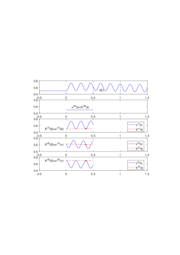
Figure 1: The top subplot gives a solution $x$ of the oscillatory problem (1) in the interval $-\tau\leq t\leq 3\tau$, $\tau=0.5$. The other subplots give the functions $x^{(\ell)}$ for $\ell=0,1,2,3$; these obviously provide all the information contained in $x$. The discontinuous lines in the last three panels depict the solution of the averaged system of ODEs (14). By definition of stroboscopic averaging, each $X^{(\ell)}$ exactly coincides with the corresponding $x^{(\ell)}$ at the initial time $t=0$. An unrealistically low value of the frequency $\Omega$ is used here so as not to clatter the plots.

In terms of the $x^{(\ell)}$, the problem (1)–(2) is given by

$$\frac{d}{dt}x^{(\ell)}(t)=$$ (11)

$$f(x^{(\ell)}(t),x^{(\ell-1)}(t),t+(\ell-1)\tau,\Omega(t+(\ell-1)\tau);\Omega),\>0\leq t\leq\tau,\>1\leq\ell\leq L,$$

in tandem with the conditions

$$x^{(\ell)}(0)=x^{(\ell-1)}(\tau),\qquad 1\leq\ell\leq L.$$ (12)

Remark 4

Note that $x^{(0)}$ is known from (9). The unknown function $x^{(1)}$ is determined from (11) with $\ell=1$ and the initial condition $x^{(1)}(0)=\varphi(0)$; once $x^{(1)}$ is known, $x^{(2)}$ is determined from (11) with $\ell=2$ and the initial condition $x^{(2)}(0)=x^{(1)}(\tau)$, etc. Thus, even though, in view of (12), the problem (11)–(12) has the appearance of a two-point boundary problem, we are really dealing with an initial-value problem (this was to be expected as (11)–(12) is just a way of writing (1)–(2)).

Obviously (11) is a highly-oscillatory system of ODEs (rather than DDEs)

$$\frac{d}{dt}{\bf x}={\bf f}({\bf x},t,\Omega t;\Omega),\qquad 0\leq t\leq\tau,$$ (13)

for the unknown function

$${\bf x}(t)=[x^{(1)}(t),\dots,x^{(L)}(t)],\qquad 0\leq t\leq\tau,$$

with values in $\mathbb{R}^{LD}$ ($x^{(0)}$ is known, see (9)). The algorithms to be described below are based on the integration of (13) with the help of SAM as described in the preceding section. If we denote by $X^{(\ell)}$ the averaged version of $x^{(\ell)}$, $\ell=1,\dots,L$, ($X^{(0)}(t)=\varphi(t-\tau)$, $0\leq t\leq\tau$) the averaged system for

$${\bf X}(t)=[X^{(1)}(t),\dots,X^{(L)}(t)],\qquad 0\leq t\leq\tau,$$

is of the form

$$\frac{d}{dt}X^{(\ell)}(t)=$$ (14)

$$F^{(\ell)}(X^{(\ell)}(t),X^{(\ell-1)}(t),\dots,X^{(0)}(t),t;\Omega),\quad 0\leq t\leq\tau,\quad 1\leq\ell\leq L,$$

where we note that $X^{(\ell+1)}$, …, $X^{(L)}$ do not appear in the right-hand side because $x^{(\ell)}$ (and therefore its averaged version $X^{(\ell)}$) does not depend on the values of the solution $x$ for $t>\ell\tau$.

Remark 5

With a terminology borrowed from linear algebra, we may say that the system (11) has a lower bidiagonal structure, while (14) is only lower triangular. The explicit formulas for the averaged system in Sanz-Serna & Zhu (2019) show that in fact for $J$ large, $X^{(\ell-2)}$,…, $X^{(0)}$ appear in the right-hand side of (14) in addition to $X^{(\ell-1)}$ and $X^{(\ell)}$.

4 Algorithms

We now introduce algorithms for the solution of (1)–(2).

4.1 Case I: the delay is an integer multiple of the period

We study first the particular case where the delay $\tau$ is an integer multiple of the period. The general situation requires algorithms with additional complications. We note that in some applications there is some freedom in choosing the exact value of the large angular frequency $\Omega$; one may then use that freedom to ensure that $\tau/T=\tau\Omega/(2\pi)$ is an integer and thus avoid the extra complications.

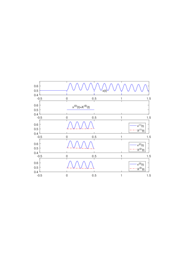
Figure 2: As Fig. 1 in the particular case where the delay $\tau$ is an integer multiple of the period $T$. The numerical approximation $X^{(\ell)}_{N}$ to $X^{(\ell)}(\tau)$ approximates $x^{(\ell)}(\tau)=x^{(\ell+1)}(0)$ and may be used as initial value to compute approximately $X^{(\ell+1)}(t)$, $0\leq t\leq\tau$, $\ell=1,\dots,L-1$.

We apply SAM, based on a macro step size $H$ of the form $\tau/N$ with $N$ a positive integer, to the integration of the $LD$ dimensional ODE system (13). While at the outset the initial condition ${\bf x}(0)$ is not known (see (12)), the triangular structure of the averaged system (14) noted in Remark 5 makes it possible to complete the application of SAM by successively computing, for $\ell=1,2,\dots,L$, the numerical approximations to the functions $X^{(\ell)}(t)$, $0\leq t\leq T$, very much as in Remark 4. One first applies SAM to the oscillatory problem for $x^{(1)}$. Because $H$ is a submultiple of $\tau$, the macrointegrator will produce an approximation $X^{(1)}_{N}$ to $X^{(1)}(\tau)=X^{(1)}(NH)$, see Figure 2. In addition we are assuming that $\tau/T\in\mathbb{N}$, so that the final time $t=\tau$ is stroboscopic and then $X^{(1)}(\tau)$ is a very accurate approximation to $x^{(1)}(\tau)$, i.e. to $x^{(2)}(0)$. Therefore $X^{(1)}_{N}$ provides an approximation to the missing initial value $x^{(2)}(0)$ and it is then possible to approximate with SAM the solution $x^{(2)}(t)$, $0\leq t\leq\tau$. Iterating this procedure one approximates all the $x^{(\ell)}(t)$, or, equivalently, the oscillatory solution $x(t)$, $0\leq t\leq t_{max}$.

Since coding SAM algorithms requires some care, it may be helpful to provide a detailed description of SAM for a particular choice of integrators and differentiation formula. This is done in Table 1 that refers to the case where the macro and microintegrators are chosen to be the familiar second-order formula of Runge that for $(d/dt)z=g(z,t)$ reads

$$z_{j+1/2}=z_{j}+\frac{\Delta t}{2}\,g(z_{j},t_{j}),\qquad z_{j+1}=z_{j}+\Delta t\,g(z_{j+1/2},t_{j}+\Delta t/2).$$

The formula needs two function evaluations per step. The algorithm uses the central difference formula (7) except when approximating $F^{(\ell)}$, $\ell=1,\dots,L$, in (14), at $t=0$ where the forward formula (6) is applied. At $t=0$ central difference are not applicable: backward microintegrations cannot be performed because the system (11) is only defined for $t\geq 0$ ($x^{(0)}$ is not defined for $t<0$, see (9)). The algorithm consists of an initialization block followed by a loop for the successive computation of the approximations to $X^{(\ell)}(t)$, $\ell=1,\dots,L$. Note the different treatment given at all the microintegrations to the third (slow time $t$) and fourth (fast rotating phase $\Omega t$) arguments of $f$; this is in agreement with Remark 2.

Table 1: SAM-RK2 Algorithm

$X^{(1)}_{0}=\varphi(0)$ % initial condition

Load history

For $\nu=0:\nu_{max}$

$x^{(0)}_{0,\nu}=\varphi(-\tau+\nu h)$, $x^{(0)}_{0,\nu+1/2}=\varphi(-\tau+(\nu+1/2)h)$,

end

For $n=1:N-1$

For $\nu=-\nu_{max}:\nu_{max}$

$x^{(0)}_{n,\nu}=\varphi(-\tau+nH+\nu h)$, $x^{(0)}_{n,\nu+1/2}=\varphi(-\tau+nH+(\nu+1/2)h)$,

end

end

Integration starts

For $\ell=1:L$

For $n=0:N-1$

Compute $F^{(\ell)}_{n}$

$t^{(\ell)}_{n}=nH+(\ell-1)\tau$ % initial time

$x^{(\ell)}_{n,0}=X^{(\ell)}_{n}$ % initial value

If $n=0$

Forward micro-integration

For $\nu=0:\nu_{max}-1$

$t^{(\ell)}_{0,\nu}=t_{0}^{(\ell)}+\nu h$, $t^{(\ell)}_{0,\nu+1/2}=t_{0}^{(\ell)}+(\nu+1/2)h$

$x^{(\ell)}_{0,\nu+1/2}=x^{(\ell)}_{0,\nu}+(h/2)f(x^{(\ell)}_{0,\nu},x^{(\ell-1)}_{0,\nu},t^{(\ell)}_{0,\nu},\Omega\nu h;\Omega)$

$x^{(\ell)}_{0,\nu+1}=x^{(\ell)}_{0,\nu}+hf(x^{(\ell)}_{0,\nu+1/2},x^{(\ell-1)}_{0,\nu+1/2},t^{(\ell)}_{0,\nu+1/2},\Omega(\nu+1/2)h;\Omega)$,

end

$F^{(\ell)}_{0}=(x^{(\ell)}_{0,\nu_{max}}-x^{(\ell)}_{0,0})/T$ % slope at 1st stage

of 1st macro-step for $X^{(\ell)}$

else

Forward micro-integration

For $\nu=0:\nu_{max}-1$,

$t^{(\ell)}_{n,\nu}=t_{n}^{(\ell)}+\nu h$, $t^{(\ell)}_{n,\nu+1/2}=t_{n}^{(\ell)}+(\nu+1/2)h$

$x^{(\ell)}_{n,\nu+1/2}=x^{(\ell)}_{n,\nu}+(h/2)f(x^{(\ell)}_{n,\nu},x^{(\ell-1)}_{n,\nu},t^{(\ell)}_{n,\nu},\Omega\nu h;\Omega)$

$x^{(\ell)}_{n,\nu+1}=x^{(\ell)}_{n,\nu}+hf(x^{(\ell)}_{n,\nu+1/2},x^{(\ell-1)}_{n,\nu+1/2},t^{(\ell)}_{n,\nu+1/2},\Omega(\nu+1/2)h;\Omega)$,

end

Backward micro-integration

For $\nu=0:\nu_{max}-1$,

$t^{(\ell)}_{n,-\nu}=t_{n}^{(\ell)}-\nu h$, $t^{(\ell)}_{n,-(\nu+1/2)}=t_{n}^{(\ell)}-(\nu+1/2)h$

$x^{(\ell)}_{n,-(\nu+1/2)}=x^{(\ell)}_{n,-\nu}-(h/2)f(x^{(\ell)}_{n,-\nu},x^{(\ell-1)}_{n,-\nu},t^{(\ell)}_{n,-\nu},-\Omega\nu h;\Omega)$

$x^{(\ell)}_{n,-(\nu+1)}=x^{(\ell)}_{n,-\nu}$

$-hf(x^{(\ell)}_{n,-(\nu+1/2)},x^{(\ell-1)}_{n,-(\nu+1/2)},t^{(\ell)}_{n,-(\nu+1/2)},-\Omega(\nu+1/2)h;\Omega)$,

end

$F^{(\ell)}_{n}=(x^{(\ell)}_{n,\nu_{max}}-x^{(\ell)}_{n,-\nu_{max}})/(2T)$ % slope at 1st stage

end

Macro-integration

$X^{(\ell)}_{n+1/2}=X^{(\ell)}_{n}+(H/2)F^{(\ell)}_{n}$, % 2nd stage of n-th macro-step

Compute $F^{(\ell)}_{n+1/2}$

$x^{(\ell)}_{n+1/2,0}=X^{(\ell)}_{n+1/2}$ % initial value

$t^{(\ell)}_{n+1/2}=(n+1/2)H+(\ell-1)\tau$ % initial time

Forward micro-integration

For $\nu=0:\nu_{max}-1$,

$t^{(\ell)}_{n+1/2,\nu}=t_{n+1/2}^{(\ell)}+\nu h,t^{(\ell)}_{n+1/2,\nu+1/2}=t_{n+1/2}^{(\ell)}+(\nu+1/2)h$

$x^{(\ell)}_{n+1/2,\nu+1/2}=x^{(\ell)}_{n+1/2,\nu}+(h/2)$

$f(x^{(\ell)}_{n+1/2,\nu},x^{(\ell-1)}_{n+1/2,\nu},t^{(\ell)}_{n+1/2,\nu},\Omega\nu h;\Omega)$

$x^{(\ell)}_{n+1/2,\nu+1}=x^{(\ell)}_{n+1/2,\nu}$

$+hf(x^{(\ell)}_{n+1/2,\nu+1/2},x^{(\ell-1)}_{n+1/2,\nu+1/2},t^{(\ell)}_{n+1/2,\nu+1/2},\Omega(\nu+1/2)h;\Omega)$,

end

Backward micro-integration

For $\nu=0:\nu_{max}-1$,

$t^{(\ell)}_{n+1/2,-\nu}=t_{n+1/2}^{(\ell)}-\nu h,t^{(\ell)}_{n+1/2,-(\nu+1/2)}=t_{n+1/2}^{(\ell)}-(\nu+1/2)h$

$x^{(\ell)}_{n+1/2,-(\nu+1/2)}=x^{(\ell)}_{n+1/2,\nu}$

$-(h/2)f(x^{(\ell)}_{n+1/2,\nu},x^{(\ell-1)}_{n+1/2,\nu},t^{(\ell)}_{n+1/2,-\nu},-\Omega\nu h;\Omega)$

$x^{(\ell)}_{n+1/2,-(\nu+1)}=x^{(\ell)}_{n+1/2,-\nu}-h\times$

$f(x^{(\ell)}_{n+1/2,-(\nu+1/2)},x^{(\ell-1)}_{n+1/2,-(\nu+1/2)},t^{(\ell)}_{n+1/2,-(\nu+1/2)},-\Omega(\nu+1/2)h;\Omega)$

end

$F^{(\ell)}_{n+1/2}=(x^{(\ell)}_{n+1/2,\nu_{max}}-x^{(\ell)}_{n+1/2,-\nu_{max}})/(2T)$ % slope at 2nd stage

Macro-step with RK2

$X^{(\ell)}_{n+1}=X^{(\ell)}_{n}+HF^{(\ell)}_{n+1/2}$

end

if $\ell<L$

$X^{(\ell+1)}_{0}=X^{(\ell)}_{N}$

end

end

Remark 6

The first-order forward difference formula is used $L$ times per run of the algorithm, regardless of the value of $H$ (or, equivalently, regardless of the number of macrosteps needed to span an interval of length $\tau$).

4.2 Case II: the delay is not an integer multiple of the period

In this case we apply SAM to the ODE system in (9) in the interval $0\leq t\leq MT$ with $M=\lfloor\tau/T\rfloor$ (see Figure 1). In the short final interval $MT\leq t\leq\tau$ (whose length is $<T$) we integrate numerically the oscillatory problem itself and for this purpose we choose the integrator and step length being used for the microintegrations. In this way the initial value $X^{(\ell)}(0)$, $\ell=2,\dots,L$, required by SAM is computed approximately as the numerical result at $t=\tau$ of the integration of the oscillatory equation for $x^{(\ell-1)}(t)$ in (9) that starts at $t=M\tau$ from the SAM approximation to $X^{(\ell-1)}(NT)\approx x^{(\ell-1)}(NT)$. The integration of the equation for $x^{(L)}(t)$ in $MT\leq t\leq\tau$ yields an approximation to $x(t_{max})$.

Remark 7

While the hypothesis $\tau/T\in\mathbb{N}$ obviously simplifies the algorithm, it is not necessary for the methods to perform satisfactorily, as the numerical experiments below will show. This should be compared with the situation for the integrator in Sanz-Serna & Zhu (2019), where, for systems of the general form (1), there is a degradation in the error behaviour if the hypothesis $\tau/T\in\mathbb{N}$ does not hold (see Remark 3 in Sanz-Serna & Zhu (2019)).

5 Error bounds

In this section we provide error bounds for the algorithms described above. We work first under the hypothesis that $\tau$ is a multiple of the period (Case I in the preceding section) and then consider the general situation. The section concludes with the presentation of some refinements. For simplicity, we assume that the macro and micro integrators are (consistent) Runge-Kutta methods.

5.1 Basic estimate: Case I

As explained above, if the delay is a multiple of the period, the integrators to be analyzed are just SAM algorithms for the system of ODEs (13). For $X^{(1)}$ the results given by our algorithms are those of macrointegrating (5) with inaccurate values of $F$. For $X^{(\ell)}$, $\ell>1$, we apply the macrointegrator with inaccurate values of $F$ and in addition with a starting value $X^{(\ell)}(0)$ that is itself not exact. Classical results of the theory of convergence of numerical ODEs show then that SAM solutions have an error bound

$$\mathcal{O}\left(H^{P}+\delta+\Omega\>\mu\right)$$ (15)

where

• The contribution $H^{P}$ ($P$ is the order of the macrointegrator) arises from the global error of the macrointegrator and would remain even if $F$ were known exactly rather than evaluated via finite differences. This contribution is uniform in $\Omega$ as $\Omega$ increases, because the stroboscopically averaged system being integrated is a polynomial in $\Omega^{-1}$ (Remark 1).

• $\delta=\delta(H,\Omega)$ is a bound for the error due to the finite-difference formula used to compute $F$.

• $\mu(h,\Omega)$ is a bound for the microintegrating error when computing approximately $\Phi_{T}(w)$ in (6) (or $\Phi_{\pm T}(w)$ in (7), etc.). The (large) factor $\Omega$ in front of $\mu$ in (15) is due to the denominator in the finite difference formulas (6), (7), etc.

We study $\mu$ assuming that the oscillatory system is written in the format (4). It is best to introduce the slow time $s=\Omega t$ that transforms (4) into

$$\frac{d}{ds}y=\Omega^{-1}f(y,s;\Omega).$$ (16)

This system has to be integrated over a forward period $0\leq s\leq 2\pi$ (or over a forward period and a backward period, etc. depending on the finite difference formula being used to recover $F$). Note that the rescaling of time is compatible with the RK discretization in the sense that the $y$ vectors produced by the algorithm when the system is integrated in the variable $t$ with step size $h$ coincide with those obtained when the system is integrated in the variable $s$ with step size $\Delta s=\Omega h$. Since we assumed at the outset that $\Omega^{-1}f$ is smooth and remains bounded together with its derivatives as $\Omega\uparrow\infty$, the microintegration errors for (16) may be estimated, uniformly in $\Omega$ as $\mu=\mathcal{O}((\Delta s)^{p})$, i.e.

$$\qquad\mu=\mathcal{O}(\Omega^{p}h^{p}),$$ (17)

where $p$ is the order of the microintegrator.

As an example we look at the algorithm in Table 1 with $P=p=2$. Second order differentiation contribute to $\delta$ with an $\Omega^{-2}$ term. Since the first-order difference formula is only used at a number of macrosteps that is fixed as $H\rightarrow 0$ (see Remark 6), its contribution to $\delta$ is $H\Omega^{-1}$. Thus we have the bound

$$\mathcal{O}\left(H^{2}+\Omega^{-2}+H\Omega^{-1}+\Omega^{3}h^{2}\right).$$

5.2 Basic estimate: Case II

In this case (15) has to be replaced by

$$\mathcal{O}\left(H^{P}+\delta+\Omega\>\mu+\nu\right),$$ (18)

where $\nu$ bounds the error introduced by the integrations of the oscillatory system in the final short interval $MT\leq t\leq\tau$. Since these are carried out in intervals of length $<T$ and there is a number $L$ of them independent of the problem parameters, from (17), we obtain the bounds

$$\nu=\mathcal{O}((\Delta s)^{p})\qquad{\rm i.e.}\qquad\nu=\mathcal{O}(\Omega^{p}h^{p}).$$ (19)

5.3 Refined microintegration estimates: $\mathcal{O}(\Omega^{-1})$ microintegration errors

There are numerous circumstances where (17) is pessimistic. An instance is given by the case where (4) is of the form

$$\frac{d}{dt}y=\Omega\>\Lambda(\Omega t)+f(y,\Omega t;\Omega),$$

with $\Lambda$ a (vector-valued) trigonometric polynomial and $f$ and its derivatives are bounded as $\Omega\uparrow\infty$.

In terms of the slow time $s$ we have

$$\frac{d}{ds}y=\Lambda(s)+\Omega^{-1}f(y,s;\Omega),$$ (20)

a system that may be seen as a perturbation of $(d/ds)y=\Lambda(s)$. For the unperturbed problem we have the following result that will be proved in Section 7.1.

Proposition 1

Let $\Lambda$ be a (vector-valued) trigonometric polynomial. A Runge-Kutta scheme applied to the initial-value problem $(d/ds)y=\Lambda(s)$, $y(0)=y_{0}$, with a constant stepsize $\Delta s=2\pi/M$ ($M$ a positive integer) gives approximations that are exact at $s=\pm 2\pi$ provided that $\Delta s$ is suffiently small.

Note that, by implication, the integrator also yields exact approximations at $s=\pm 4\pi$, $s=\pm 6\pi$, etc. Thus the computation of the values of $\Phi_{\pm kT}$ used in the finite-difference formulas will be free from error and, for the unperturbed problem, $\mu=0$. From the proposition it may be expected that for the perturbed system (20) the microintegration error after a whole number of periods will approach 0 as $\Omega\uparrow\infty$ with $\Delta s$ fixed. In fact in this case (17) may be replaced by

$$\mu=\Omega^{-1}\mathcal{O}((\Delta s)^{p})\qquad{\rm or}\qquad\mu=\mathcal{O}(\Omega^{p-1}h^{p}),$$ (21)

an estimate that will be established in Section 7.2.

5.4 Refined microintegration estimates: $\mathcal{O}(\Omega^{-2})$ microintegration errors

An even more favourable situation holds when in (4) $f$ and its derivatives remain bounded as $\Omega\uparrow\infty$ and as a function of its second argument is a trigonometric polynomial. According to (16), for $0\leq s\leq 2\pi$, $y(s)-y(0)=\mathcal{O}(\Omega^{-1})$ and we may consider a decomposition

$$\frac{d}{ds}y=\Omega^{-1}f(y(0),s;\Omega)+\Omega^{-1}\Big{(}f(y,s;\Omega)-f(y(0),s;\Omega)\Big{)}.$$

For the unperturbed system $(d/ds)y=\Omega^{-1}f(y(0),s;\Omega)$ the output of the microintegrations is exact in view of the preceding proposition; the perturbation is $\mathcal{O}(\Omega^{-2})$ for $0\leq s\leq 2\pi$ and (17) may be replaced by the improved estimate (Section 7)

$$\mu=\Omega^{-2}\mathcal{O}((\Delta s)^{p})\qquad{\rm or}\qquad\mu=\mathcal{O}(\Omega^{p-2}h^{p}).$$ (22)

We emphasize that the improved bounds for $\mu$ we have just discussed hold because the integration of the unperturbed problem is exact after a whole number of periods. The bound (19) cannot be improved similarly because there the integration is not carried out for a whole number of periods.

6 Numerical experiments

We now report numerical experiments based on SAM. They are based on the following algorithms:

Table 2: Coefficients of methods RK3 (left) and RK4 (right).

$\begin{array}[]{c|ccc}&&&\\[6.0pt] 0&&&\\[6.0pt] \frac{1}{3}&\frac{1}{3}&&\\[6.0pt] \frac{2}{3}&0&\frac{2}{3}&\\[6.0pt] \hline\cr\\[-6.0pt] &\frac{1}{4}&0&\frac{3}{4}\end{array}\qquad\qquad\begin{array}[]{c|cccc}0&&&&\\[6.0pt] \frac{1}{2}&\frac{1}{2}&&&\\[6.0pt] \frac{1}{2}&0&\frac{1}{2}&&\\[6.0pt] 1&0&0&1&\\[6.0pt] \hline\cr\\[-6.0pt] &\frac{1}{6}&\frac{2}{6}&\frac{2}{6}&\frac{1}{6}\end{array}$

1. SAM-RK3. This is a SAM algorithm, similar to that in Table 1, that uses the well-known third order RK method in Table 2 as macro and microintegrator. We approximate $F$ by means of the differentiation formula with $\mathcal{O}(\Omega^{-3})$ errors based on function values at $-2T$, $-T$, $0$, $T$. At $t=0$, where backward microintegrations are not possible, we use the $\mathcal{O}(\Omega^{-3})$ forward differentiation formula based on function values at $0$, $T$, $2T$, $3T$.

2. SAM-RK4. A SAM algorithm, similar to that in Table 1, that uses the ‘classical’ order four RK method (see Table 2) as macro and microintegrator. We approximate $F$ by means of the well-known differentiation formula based on function values at $\pm T$, $\pm 2T$ ($\mathcal{O}(\Omega^{-4})$ errors). For the first-stage of the formula at $t=0$, where backward microintegrations are not possible we use the $\mathcal{O}(\Omega^{-4})$ formula based on function values at $0$, $T$, $2T$, $3T$, $4T$. In addition the fourth stage requires values of $F$ at the end point $t=\tau$ and for those we use the $\mathcal{O}(\Omega^{-4})$ formula based on $-4T$, $-3T$, $-2T$, $-T$, $0$.

3. SS-Z. This is the integrator introduced in (Sanz-Serna & Zhu, 2019) that is not based on rewriting the system as an ODE.

Experiments using the method in Table 1 were also conducted, but will not be reported as its performance is very similar to that of SS-Z. In fact, the number of possible combinations of integrators and differentiation formulas is bewildering. The choices used here are meant to illustrate the possibilities of the SAM idea and we have not attempted to identify the most efficient combinations.

6.1 Test problems

We have integrated the two test problems used in (Sanz-Serna & Zhu, 2019). The first is given by (3) together with the history information $x_{1}(t)=0.5$, $x_{2}(t)=2.0$, for $-\tau\leq t\leq 0$. The constants in the model have the values $\alpha=2.5$, $\beta=2$, $A=0.1$, $\omega=0.1$, $B=4.0$, $\tau=0.5$. This leads to an ODE system that satisfies the hypotheses in Section 5.4 so that the estimate (22) holds.

The second test problem is the following more demanding variant of (3):

$$\frac{dx_{1}}{dt} = \frac{\alpha}{1+x_{2}^{\beta}}-x_{1}(t-\tau)+A\sin(\omega t)+\hat{B}\Omega\sin(\Omega t),$$ (23)

$$\frac{dx_{2}}{dt} = \frac{\alpha}{1+x_{1}^{\beta}}-x_{2}(t-\tau),$$

with $\hat{B}=0.1$ and all other constants and the initial history as for (3). Now the amplitude of the fast forcing grows linearly with $\Omega$ and, as a result, the solution undergoes fast oscillations of amplitude $O(1)$, as $\Omega\rightarrow\infty$ (rather than $O(\Omega^{-1})$ as it is the case for (3)). Clearly (23) leads to a system of ODEs of the form (20) and estimate (21) holds.

6.2 Results: case I

We first set $\Omega=8\pi,16\pi,\ldots$, so that the delay $\tau=0.5$ is an integer multiple of the fast period $T=2\pi/\Omega$.

Table 3: Maximum errors at stroboscopic times in $x_{1}$ for SAM-RK4 with respect to the reference solution for problem (3)

N	$\Omega=16\pi$	$\Omega=32\pi$	$\Omega=64\pi$	$\Omega=128\pi$	$\Omega=256\pi$	$\Omega=512\pi$	$\Omega=1024\pi$
1	1.18(-3)	6.17(-4)	3.48(-4)	1.86(-4)	9.41(-5)	4.50(-5)	1.95(-5)
2	***	3.01(-5)	1.70(-5)	9.09(-6)	4.62(-6)	2.23(-6)	9.98(-7)
4	***	***	1.00(-6)	5.40(-7)	2.77(-7)	1.35(-7)	6.18(-8)
8	***	***	***	3.34(-8)	1.72(-8)	8.44(-9)	3.89(-9)
16	***	***	***	***	1.12(-9)	5.26(-10)	2.23(-10)
32	***	***	***	***	***	2.93(-11)	1.87(-11)
64	***	***	***	***	***	***	2.30(-11)

6.2.1 Test problem (3)

For each value of $\Omega$, we have first computed a reference solution of the problem in the interval $[0,2]$ using the Matlab function dde23 with relative and absolute tolerances equal to $10^{-11}$; errors have been measured with respect to this reference solution. Notice that the interval $[0,2]$ includes the locations $t=\ell\times\tau$ for $0\leq\ell\leq 4$. When studying vibrational resonances in (3) the interest lies in much longer time intervals, but we have not used them in our study due to the extremely high cost of finding the reference solution with dde23 when $\Omega$ is large. We have run the algorithms with macro-stepsize $H=\tau/N$ and micro-stepsize $h=T/(2N)$ for $N=1,2,4,\ldots$ This implies that when $N$ is doubled, both the macro stepsize and the micro stepsize are divided by two and, consequently, the computational cost, which is independent of $\Omega$, is multiplied by four.

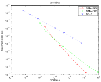
Figure 3: Maximum error at stroboscopic times, with respect to the reference solution, in the first component of SAM-RK4 (diamonds), SAM-RK3 (squares) and SS-Z (triangles) versus CPU time for $\Omega=1024\pi$. Errors for SAM-RK4 come from the last column in Table 3.

Table 3 shows, for the first component of the solution, maximum errors at stroboscopic times in the interval $0\leq t\leq 2$ when the integration is performed with SAM-RK4. Stars denote combinations $(N,\Omega)$ for which the numerical solution has not been computed because the macrostepsize $H$ is not significantly larger than the period $T$ and the heterogeneous multiscale approach does not make sense. Note that entries in the table below, say, $10^{-11}$ may not be reliable due to the accuracy we used in computing the reference solution. According to the estimates in the preceding section, for SAM-RK4 there is an $H^{4}$, i.e. $N^{-4}$, contribution to the error bound (15) arising from the macrointegrator, an $\Omega^{-4}$ contribution arising from the use of finite differences and $\Omega\mu$ may be bounded by $\Omega^{3}h^{4}$, or $\Omega^{-1}N^{-4}$. The numbers in the table have a clear $\Omega^{-1}N^{-4}$ behaviour, which shows that the error is mainly due to the microintegrations. For the values of $\Omega$ under consideration the finite differences employed are virtually exact and, in addition, the error arising from the macrointegrator is also negligible (the averaged solution varies very little in the short integration interval).

For SAM-RK3 the contributions to (15) are respectively $H^{3}$, $\Omega^{-3}$ and $\Omega^{2}h^{3}$. The results show an $\Omega^{2}h^{3}$, i.e. $\Omega^{-1}N^{-3}$, behaviour (which corresponds to the error being dominated by the microintegrations) and will not be reproduced here. Error bounds and numerical results for SS-Z may be seen in (Sanz-Serna & Zhu, 2019). We plot in Figure 3 an efficiency diagram comparing these three integrators. The figure represents, in doubly-logarithmic scale, the maximum error in $x_{1}$ at stroboscopic times versus the CPU time when $\Omega=1024\pi$. We first observe that the slopes of the different lines are close to $-1$ (triangles), $-3/2$ (squares) and $-2$ (diamonds). As mentioned above, due to our choice of $H$ and $h$ (i.e. $H=\tau/N$, $h=T/(2N)$, $N=1,2,\ldots,128$), the computational cost is multiplied by $2^{2}$ when $N$ is doubled and, consequently, the slopes observed in Figure 3 correspond to a dependence on $N$ of the form $N^{-2}$, $N^{-3}$, $N^{-4}$, in agreement with the bounds of the preceding section (and those for SS-Z presented in Sanz-Serna & Zhu (2019)). Comparing the three integrators, we also conclude that for errors larger than $10^{-4}$, SS-Z is the most efficient, for errors between $10^{-6}$ and $10^{-4}$ SAM-RK3 is preferable, and for errors smaller than $10^{-6}$ the more accurate SAM-RK4 requires the smallest CPU time. Similar conclusions may be drawn for other values of $\Omega$ (but the range of errors where one method is better than the others varies slightly with $\Omega$).

6.2.2 Test problem (23)

Table 4: Maximum errors at stroboscopic times in $x_{1}$ for SAM-RK4 with respect to the reference solution for problem (23)

N	$\Omega=16\pi$	$\Omega=32\pi$	$\Omega=64\pi$	$\Omega=128\pi$	$\Omega=256\pi$	$\Omega=512\pi$
1	1.62(-3)	1.64(-3)	1.65(-3)	1.65(-3)	1.65(-3)	1.65(-3)
2	***	8.26(-5)	8.29(-5)	8.29(-5)	8.29(-5)	8.29(-5)
4	***	***	4.72(-6)	4.73(-6)	4.73(-6)	4.73(-6)
8	***	***	***	2.93(-7)	2.93(-7)	2.93(-7)
16	***	***	***	***	1.83(-8)	1.83(-8)
32	***	***	***	***	***	1.15(-9)

Table 4 corresponds to (23) integrated with SAM-RK4. Errors for $\Omega=1024\pi$ are not reported because, with our facilities, the computation of the reference solution with dde23 would take several days. The error bounds are different from those for (3) because for this tougher problem the microintegration bound is as in (21) so that the impact $\Omega\mu$ of the microintegration is now $\Omega^{4}h^{4}$ or $N^{-4}$; this impact is then $\Omega$ independent. In fact, the main difference observed when comparing Tables 3 and  4, is that in Table 4 errors along each row stay constant while in Table 3 they decrease as $\Omega$ increases as discussed above.

On the other hand, we observe that the same macro stepsizes used to integrate (3) can be successfully used in this new, more challenging problem and lead to errors that are not widely different; this should be compared with the direct integration of the oscillatory problem with dde23 where the costs for (23) are much higher than those for (3).

6.3 Results: case II

We consider again the integration of (3) and (23) but now set $\Omega=25,50,\ldots$ These values are not very different from the values used in the preceding section, but now the delay $\tau=0.5$ is not an integer multiple of the period $T=2\pi/\Omega$ of the fast oscillations. The integrators SAM-RK3, SAM-RK4 and SS-Z have been run with macro-stepsize $H=H_{max}/N$, $N=1,2,4,\ldots$ with $H_{max}=MT$, $M=\lfloor\tau/T\rfloor$. The micro-stepsize is again $h=T/(2N)$. As explained in Section 4.2, in order to get solution values at integer multiples of $\tau$, each macrointegration from $0$ to $MT$ is followed by a short integration of the oscillatory problem from $MT$ to $\tau$. We only report a representative small sample of the experiments we performed.

Table 5: Errors at $t_{max}$ in $x_{1}$ for SAM-RK4 with respect to the reference solution for problem (3)

N	$\Omega=50$	$\Omega=100$	$\Omega=200$	$\Omega=400$	$\Omega=800$	$\Omega=1600$
1	3.98(-3)	3.93(-3)	2.27(-3)	3.91(-4)	3.99(-4)	4.82(-5)
2	***	2.16(-4)	1.55(-4)	2.21(-5)	1.84(-5)	3.37(-6)
4	***	***	5.14(-6)	1.32(-6)	9.01(-7)	2.07(-7)
8	***	***	***	8.79(-8)	5.46(-8)	1.71(-8)
16	***	***	***	***	3.10(-9)	1.05(-9)
32	***	***	***	***	***	5.56(-11)

Table 5 contains the errors in the first component of the solution of (3) at the final time $t_{max}=4\tau$, with respect to the reference dde23 solution when the integration is performed with SAM-RK4. In (18), $P$, $\delta$ and $\mu$ are as in Case I and the additional contribution $\nu$ from the short integrations is $(\Omega h)^{4}$, i.e. $N^{-4}$. The errors displayed in this table show a clear $N^{-4}$ behaviour along the columns. However the variation with $\Omega$ is now not so regular as we found in Table 3 for Case I, no doubt because now changing $\Omega$ changes the phase of the oscillation at the final time, where errors are measured.

Finally, we report in Table 6 errors in the first component of the solution of the challenging problem (23). This is to be compared with Table 4; again the error behaviour as a function of $\Omega$ is now more irregular, but the methodology outlined in this paper finds no difficulty in accurately integrating the problem.

Table 6: Errors at $t_{max}$ in $x_{1}$ for SAM-RK4 with respect to the reference solution for problem (23)

	N	$\Omega=50$	$\Omega=100$	$\Omega=200$	$\Omega=400$	$\Omega=800$
	1	4.86(-3)	9.97(-3)	1.20(-2)	3.19(-3)	8.30(-3)
	2	***	5.46(-4)	8.01(-4)	2.46(-4)	3.80(-4)
	4	***	***	2.63(-5)	1.45(-5)	1.89(-5)
	8	***	***	***	9.33(-7)	1.15(-6)
	16	***	***	***	***	6.56(-8)

7 Proofs and additional results

We conclude the paper by supplying the proofs of some results presented in Section 5. We also present some extensions of those results.

7.1 Proof of Proposition 1

It is clearly sufficient to carry out the proof for the particular case of the scalar differential equation $dy/ds=\exp(iks)$, with $k\neq 0$ an integer. The true solution has the value $y_{0}$ at $s=2\pi$. If $\{b_{j}\}_{j=1}^{\sigma}$ and $\{c_{j}\}_{j=1}^{\sigma}$ are the weights and abscissas of the RK formula and $M\Delta s=2\pi$, the numerical solution at $s=2\pi$ is

$$y_{M}=y_{0}+\Delta s\sum_{m=0}^{M-1}\sum_{j=1}^{\sigma}b_{j}\exp(ik((m+c_{j})\Delta s)).$$

Hence

$$y_{M}-y_{0}=\Delta s\sum_{j=1}^{\sigma}b_{j}\exp(ikc_{j}\Delta s)\sum_{m=0}^{M-1}\exp(ikm\Delta s).$$

If $\Delta s$ is sufficiently small $\exp(ik\Delta s)\neq 1$ and the inner sum takes the value

$$\frac{\exp(ikM\Delta s)-1}{\exp(ik\Delta s)-1}=\frac{\exp(i2k\pi)-1}{\exp(ik\Delta s)-1}=0.$$

As a result $y_{M}=y_{0}$, i.e. $y_{M}$ coincides with the true solution.

Remark 8

If $\exp(ik\Delta s)=1$ with $k\neq 0$, then $\exp(iks)=1$ at all mesh points $s=0,\Delta s,2\Delta s,\dots$, i.e. the oscillatory function $\exp(iks)$ is an alias of the constant function $1$. In that case, the inner sum equals $M$ and

$$y_{M}-y_{0}=2\pi\sum_{j=1}^{\sigma}b_{j}\exp(ikc_{j}\Delta s).$$

Thus the RK solution is not exact at $s=2\pi$.

7.2 Proof of the improved micro-integration estimates

Let us prove the error bound (21); the proof of (22) follows the same pattern and will not be given. We start by noting that the solution of the initial value problem given by $y(0)=y_{0}$ and (20) may be written as $y=v+z$, where the pair $(v,z)$ is the solution of the extended problem

$$\frac{dv}{ds}=\Lambda(s),\qquad v(0)=0,$$ (24)

$$\frac{dz}{ds}=\Omega^{-1}f(v+z,s;\Omega),\qquad z(0)=y_{0}.$$ (25)

By writing the equations that define the RK solution, it is straightforward to check that, similarly, the RK trajectory $y_{0}$, $y_{1}$, …, $y_{M}$ is given by $y_{m}=v_{m}+z_{m}$, $m=0,\dots,M$, where $(v_{0},z_{0})$,…, $(v_{M},z_{M})$ is the RK trajectory for the initial value problem (24)–(25). From the proposition we know that, for $\Delta s$ small, the RK approximation to the $v$ component of the extended solution is exact at $s=2\pi$, i.e. $v_{M}=v(2\pi)$ and the proof concludes by showing that the RK errors in the $z$ component $z_{M}-z(2\pi)$ possesses an $\Omega^{-1}\mathcal{O}((\Delta s)^{p}))$ bound.

The RK discretization of (24)–(25) is of the form

$$v_{m+1} = v_{m}+\Delta sF(m\Delta s,\Delta s),$$ (26)

$$z_{m+1} = z_{m}+\Delta s\Omega^{-1}G(v_{m}+z_{m},m\Delta s,\Delta s;\Omega),$$ (27)

where $F$ and $G$ are suitable increment functions; $G$ and its derivatives are bounded as $\Omega\uparrow\infty$. Clearly, for the quadrature in (24), $\max_{m}|v_{m}-v(m\Delta s)|=\mathcal{O}((\Delta s)^{p})$, with the constant implied in the $\mathcal{O}$ notation independent of $\Omega$. For the $z$ component we define the local error $\eta_{m}$ by

$$z((m+1)\Delta s)=z(m\Delta s)+\Delta s\Omega^{-1}G(v(m\Delta s)+z(m\Delta s),m\Delta s,\Delta s;\Omega)+\eta_{m}.$$

Since the right hand-side of the equation in (25) has a prefactor $\Omega^{-1}$, the same happens for all the associated elementary differentials Butcher (2016); hlw in the expansion of $z$ and as a consequence $\max_{m}|\eta_{m}|=\Omega^{-1}\mathcal{O}((\Delta s)^{p+1})$ (again the implied constant is $\Omega$-independent). Subtraction of the last display from (27) leads to ($C$ denotes an $\Omega$-independent Lipschitz constant)

$$|z_{m+1}-z((m+1)\Delta s)| \leq |z_{m}-z(m\Delta s)|$$

$$+\Delta s\Omega^{-1}C\Big{(}|v_{m}-v(m\Delta s)|+|z_{m}-z(m\Delta s)|\Big{)}$$

$$+|\eta_{m}|$$

$$= (1+\Delta s\Omega^{-1}C)|z_{m}-z(m\Delta s)|+\Delta s\Omega^{-1}\mathcal{O}((\Delta s)^{p}),$$

and recursively we arrive at $\max_{m}|z_{m}-z(m\Delta s)|=\Omega^{-1}\mathcal{O}((\Delta s)^{p})$ and the proof is ready.

7.3 Extensions

The improved bounds (21) and (22) are based on Proposition 1. This proposition does not hold if $\Lambda(s)$ is merely a smooth $2\pi$-periodic function rather than a trigonometric polynomial. In fact, if $\Lambda$ contains infinitely many Fourier modes, then for each choice of $\Delta s=2\pi/M$ there will be modes $\exp(iks)$ that are alias of the function $1=\exp(i0s)$ and therefore are not exactly integrated as we know from Remark 8. However for $\Lambda$ smooth and $2\pi$-periodic it is still possible to derive superconvergence results that show that the RK solution with $\Delta s=2\pi/M$ is more accurate at $s=2\pi$ than it is for $s<2\pi$. Those results are derived by decomposing the solution in a Fourier series. If $\Lambda$ has derivatives of all orders, then the RK error at the final point may be proved to be $\mathcal{O}((\Delta s)^{q})$ for arbitrary $q>0$. Under analyticity assumptions, the error may decrease exponentially. The situation is very similar to that of the trapezoidal rule studied in Trefethen & Weideman (2014). (In fact, due to the periodicity, the sum $\sum_{m=0}^{M-1}\exp(ikm\Delta s)$ we encountered in Section 7.1 may be written in trapezoidal form ${\sum_{m=0}^{\prime\prime M}}\exp(ikm\Delta s)$, where the double prime indicates that the first and last terms are halved.) By using the technique in Section 7.2 the superconvergence results for $(d/ds)y=\Lambda(s)$ give rise to improved micro-integration bounds for problems of the form (20) with $f$ bounded and $\Lambda$ $2\pi$-periodic or for the case where in (4) $f$ and its derivatives remain bounded as $\Omega$ increases.

References

- Ariel et al. (2009) Ariel, G., Engquist, B., Tsai, R.: A multiscale method for highly oscillatory ordinary differential equations with resonance. Math. Comput. 78, 929–956 (2009)
- Butcher (2016) Butcher, J.C.: Numerical methods for ordinary differential equations, (3rd edn.) John Wiley & Sons, Chichester (2016)
- Calvo et al. (2011a) Calvo, M.P., Chartier, Ph., Murua A., Sanz-Serna, J.M.: Numerical stroboscopic averaging for ODEs and DAEs. Appl. Numer. Math. 61, 1077–1095 (2011)
- Calvo et al. (2011b) Calvo, M.P., Chartier, Ph., Murua, A., Sanz-Serna, J.M.: A stroboscopic method for highly oscillatory problems. In: Numerical Analysis and Multiscale Computations (B. Engquist, O. Runborg & R. Tsai eds.) Springer, New York, pp. 73–87 (2011)
- Calvo & Sanz-Serna (2010) Calvo, M.P., Sanz-Serna, J.M.: Heterogeneous Multiscale Methods for mechanical systems with vibrations. SIAM J. Sci. Comput. 32, 2029–2046 (2010)
- Chartier et al. (2010) Chartier, Ph., Murua, A., Sanz-Serna, J.M.: Higher-order averaging, formal series and numerical integration I: B-series. Found. Comput. Math. 10, 695–727 (2010)
- Chartier et al. (2012) Chartier, Ph., Murua, A., Sanz-Serna, J.M.: Higher-order averaging, formal series and numerical integration II: the quasi-periodic case. Found. Comput. Math. 12, 471–508 (2012)
- Chartier et al. (2015) Chartier, Ph., Murua, A., Sanz-Serna, J.M.: Higher-order averaging, formal series and numerical integration III: error bounds. Found. Comput. Math. 15, 591–612 (2015)
- Daza et al. (2013a) Daza, A., Wagemakers, A., Rajasekar, S., Sanjuán, M.A.F.: Vibrational resonance in a time-delayed genetic toggle switch. Commun. Nonlinear Sci. Numer. Simul. 18, 411–416 (2013)
- E (2003) E, W.: Analysis of the heterogeneous multiscale method for ordinary differential equations. Comm. Math. Sci. 1, 423–436 (2003)
- E & Engquist (2003) E, W., Engquist, B.: The heterogeneous multiscale methods. Comm. Math. Sci. 1, 87–132 (2003)
- E et al. (2007) E, W., Engquist, B., Li, X., Ren, W., Vanden-Eijnden, E.: The heterogeneous multiscale method: a review. Commun. Comput. Phys. 2, 367–450 (2007)
- Engquist & Tsai (2005) Engquist, B., Tsai, Y.H.: Heterogeneous multiscale methods for stiff ordinary differential equations. Math. Comput. 74, 1707–1742 (2005)
- Gardner et al. (2000) Gardner, T.S., Cantor, C.R., Collins, J.J.: Construction of a genetic toggle switch in Escherichia coli. Nature 403, 393–342 (2000)
- (15) Hairer, E., Lubich, Ch., Wanner, G.: Geometric Numerical Integration (2nd edn.) Springer, Berlin (2006)
- Isaacson & Keller (1966) Isaacson, E., Keller, H.B.: Analysis of Numerical Methods. John Wiley & Sons, New York 1966
- Landa & McClintock (2000) Landa, P.S., McClintock, P.V.E.: Vibrational resonance. J. Phys. A 33, L433 (2000)
- Li et al. (2007) Li, J., Kevrekidis, P.G., Gear, C.W., Kevrekidis, I.G.: Deciding the nature of the coarse equation through microscopic simulations: the baby-bathwater scheme. SIAM Rev. 49, 469–487 (2007)
- Murua & Sanz-Serna (2016) Murua, A., Sanz-Serna, J.M.: Vibrational resonance: a study with high-order word-series averaging. Applied Mathematics and Nonlinear Sciences 1, 239-246 (2016)
- Murua & Sanz-Serna (2018) Murua, A., Sanz-Serna, J.M.: Averaging and computing normal forms with word series algorithms. In: Discrete Mechanics, Geometric Integration and Lie-Butcher Series (K. Ebrahimi-Fard & M. Barbero Liñán eds.) Springer, Berlin, pp. 115–137 (2018)
- Murua & Sanz-Serna (2019) Murua, A., Sanz-Serna, J.M.: Hopf algebra techniques to handle dynamical systems and numerical integrators. In: Proceedings of the 2016 Abel Symposium. Springer, to appear (2019)
- Sanz-Serna (1985) Sanz-Serna, J.M.: Stability and convergence in numerical analysis I: Linear problems-A simple, comprehensive account. In: Nonlinear Differential Equations (J. K. Hale & P. Martinez-Amores eds.) Pitman, Boston, pp. 64–113 (1985)
- Sanz-Serna (2009) Sanz-Serna, J.M.: Modulated Fourier expansions and heterogeneous multiscale methods. IMA J. Numer. Anal. 29, 595–605 (2009)
- Sanz-Serna & Zhu (2019) Sanz-Serna, J.M., Zhu, Beibei: A stroboscopic averaging algorithm for highly oscillatory delay problems. IMA J. Numer. Anal. to appear (2019)
- Trefethen & Weideman (2014) Trefethen, L.N., Weideman, J.A.C.: The exponentially convergent trapezoidal rule. SIAM Rev. 56, 385–458 (2014)