A microcanonical entropy correcting finite-size effects in small systems

Abstract

In a recent paper [Franzosi, Physica A 494, 302 (2018)], we have suggested to use of the surface entropy, namely the logarithm of the area of a hypersurface of constant energy in the phase space, as an expression for the thermodynamic microcanonical entropy, in place of the standard definition usually known as Boltzmann entropy. In the present manuscript, we have tested the surface entropy on the Fermi-Pasta-Ulam model for which we have computed the caloric equations that derive from both the Boltzmann entropy and the surface entropy. The results achieved clearly show that in the case of the Boltzmann entropy there is a strong dependence of the caloric equation from the system size, whereas in the case of the surface entropy there is no such dependence. We infer that the issues that one encounters when the Boltzmann entropy is used in the statistical description of small systems could be a clue of a deeper defect of this entropy that derives from its basic definition. Furthermore, we show that the surface entropy is well founded from a mathematical point of view, and we show that it is the only admissible entropy definition, for an isolated and finite system with a given energy, which is consistent with the postulate of equal a-priori probability.

I Introduction

The thermodynamics of an isolated system is described by the microcanonical ensemble, in which the averages of all the physical quantities are derived by the entropy. Thus, the starting point for the statistical description of any isolated system is the definition for the entropy. In the case of a classical Hamiltonian system, there are two accepted choices: the Boltzmann entropy and the Gibbs entropy. Recently, a third entropy definition has been proposed in Franzosi (2018), there the surface entropy has been defined similarly to the Boltzmann entropy but without a limit for a spread of energy that vanishes. In Ref. Franzosi (2018) we have proved that in the limit of a large number of degrees of freedom, the surface entropy predicts the same results as the Boltzmann entropy, included the possibility to observe negative temperatures. In the present work we show that, on the contrary, in the case of small systems these entropies can be inequivalent. Here we show, in fact, that the surface entropy has properties which make it an attractive definition for small systems. In particular, in Sec. III is reported the main result: We derive the surface entropy from first principles, we show that this definition is the only admissible for a classical isolated system with a given energy, which is consistent with the postulate of equal a-priori probability. Before this, in Sec. II, we report results of simulations on a Fermi-Pasta-Ulam non-linearly coupled oscillator chain, that show that in the case of the surface entropy there is not an appreciable dependence of the caloric equation from the system size, whereas, in the case of the Boltzmann entropy there is an evident dependence.

Let $H(x)$ be a classical Hamiltonian describing an autonomous many-body system of $n$ interacting particles in $d$ spatial dimensions. Let the coordinates and canonical momenta $(q_{1}\ldots,p_{1},\ldots)$ be represented as $N$-components vectors $x\in\mathbb{R}^{N}$, with $N=2nd$. Let $M_{E}=\left\{x\in\mathbb{R}^{N}|H(x)\leq E\right\}$ be the set of phase-space states with total energy less than or equal to $E$. The Gibbs entropy for this system is

$$S_{G}(E)=\kappa_{B}\ln\Omega(E)\,,$$ (1)

where $\kappa_{B}$ is the Boltzmann constant and

$$\Omega(E)=\dfrac{1}{h^{nd}}\int d^{N}x\Theta(E-H(x))$$ (2)

is the number of states with energy below $E$, $h$ is the Planck constant and $\Theta$ is the Heaviside function. Conversely, the Boltzmann entropy pertains to the energy-level sets $\Sigma_{E}=\left\{x\in\mathbb{R}^{N}|H(x)=E\right\}$ and is given in terms of $\omega(E)=\partial\Omega/\partial E$, according to

$$S_{B}(E)=\kappa_{B}\ln\left(\omega(E)\Delta\right)\,,$$ (3)

where the constant $\Delta$ has dimension of energy and makes the argument of the logarithm dimensionless, and

$$\omega(E)=\dfrac{1}{h^{nd}}\int d^{N}x\delta(E-H(x))\,,$$ (4)

is expressed in terms of the Dirac $\delta$ function. Remarkably, in the case of smooth level sets $\Sigma_{E}$, $\omega(E)$ can be cast in the following form Rugh (1997); Franzosi (2011, 2012)

$$\omega(E)=\dfrac{1}{h^{nd}}\int_{\Sigma_{E}}\dfrac{m^{N-1}(\Sigma_{E})}{\|\nabla H(x)\|}\,,$$ (5)

where $m^{N-1}(\Sigma_{E})$ is the metric induced from $\mathbb{R}^{N}$ on the hypersurface $\Sigma_{E}$ and $\|\nabla H(x)\|$ is the norm of the gradient of $H$ at $x$. Finally, in Ref. Franzosi (2018) we have proposed the definition of the surface entropy

$$S(E)=\kappa_{B}\ln\left(\sigma(E)\Lambda^{1/2}\right)\,,$$ (6)

where the constant $\Lambda$ has the dimension of action and makes the argument of the logarithm dimensionless and

$$\sigma(E)=\dfrac{1}{h^{nd}}\int_{\Sigma_{E}}m^{N-1}(\Sigma_{E})\,,$$ (7)

is the measure of $\Sigma_{E}$. Very recently, the long-standing debate on which one is the correct entropy definition, between the Boltzmann’s and the Gibb’s one, has became a topical one after the papers of Refs. Dunkel and Hilbert (2013); Hilbert et al. (2014); Hänggi et al. (2016), in which it has been argued that the Gibbs entropy yields a consistent thermodynamics, whereas the Boltzmann entropy would have some consistency issues. This fact, indeed, would have dramatic consequences about the foundations of statistical mechanics. For instance, the notion of negative temperatures is a well-founded concept in the Boltzmann description, whereas it is forbidden in the Gibbs description. On the contrary, in Refs. Buonsante et al. (2016, 2017), we have shown that the Boltzmann entropy provides a consistent description of the microcanonical thermostatistics of macroscopic systems, and, consequently, negative temperatures are a well-posed concept. For instance, in Ref. Buonsante et al. (2016) we show that, in the thermodynamic limit, the Gibbs and Boltzmann temperatures do coincide when the latter is positive whereas the inverse Gibbs temperature is identically null in the region where Boltzmann provides negative values for the temperature. This means that in correspondence of the energies where $\beta_{B}$ is negative, none microcanonical description based on the Gibbs entropy is possible, albeit the region of energies corresponding to $\beta_{B}<0$ is absolutely accessible to microscopic dynamics.

Nonetheless, the relation between the total energy and the inverse temperature, $E(\beta)$, for instance in the simple case of an isolated ideal gas system, derived with the standard Boltzmann entropy, is not an extensive quantity. Although this fact does not represent a problem in the case of macroscopic systems, since the correction to the extensive behaviour is of the order of $1/(nd)$, it may be an issue in the case of small systems since the measure of temperature (and other thermodynamic quantities) in such systems could be inaccurate. In order to overcome such issues, we have recently proposed the surface entropy (6), that reproduces the same results as the Boltzmann entropy for systems with a macroscopic number of particles but it predicts the correct extensivity for the total energy derived by the caloric equation, in the case of small systems Franzosi (2018). Therefore, in our opinion, the definition (6) represents a valid candidate for the solution of the problem regarding the correct statistical description of isolated finite systems.

Actually, a check of consistency of the surface entropy is lacking and the purpose of the present manuscript is, indeed, to provide a mathematical foundation of this entropy definition. Before starting such a discussion, we report the results of numerical simulations.

II Paradigmatic evidences

As an example, we consider the celebrated Fermi-Pasta-Ulam (FPU) $\beta$-model Fermi et al. (1965), described by the Hamiltonian

$$H=\sum^{n}_{j=1}\left[\dfrac{1}{2}p^{2}_{j}+\dfrac{1}{2}(q_{j}-q_{j+1})^{2}+\dfrac{\mu}{4}(q_{j}-q_{j+1})^{4}\right]\,,$$ (8)

where we have taken periodic boundary conditions. The FPU is a nonlinear chaotic system and it has been largely used as a toy model since the first numerical experiment by Fermi and co-authors. This apparently simple system has unveiled intriguing behaviours as to the dynamical instability Pettini et al. (2005a) and this is one of the reasons for its interest. Within the present study on the surface entropy, such a model exhibits two-fold convenience. Firstly, in this case, the statistical ensembles equivalence holds true and thermodynamic quantities derived in the canonical and in the microcanonical ensemble will agree in the thermodynamic limit. Secondly, the kinetic energy has the standard form and this permits to perform some analytical calculations Pearson et al. (1985). In addition, Hamiltonian (8) is unbounded from above and therefore the thermodynamics derived from the Boltzmann and Gibbs entropy are consistent Buonsante et al. (2016), at least in the case of macroscopic number of degrees of freedom. In the following, we report on a numerical analysis performed on the FPU model in which we have measured appropriate quantities along the dynamics generated by Hamiltonian (8), in order to derive the caloric equation either from the Boltzmann entropy and from the surface entropy. In order to test the reliability of the two entropy definitions, the simulations have been performed for several system sizes.

As far as the standard Boltzmann entropy, the form of Hamiltonian (8) allows using the Laplace-transform technique Pearson et al. (1985) in order to measure the Boltzmann inverse temperature

$$\beta_{B}=\left(\dfrac{n}{2}-1\right)\langle K^{-1}\rangle_{\mu c}\,,$$ (9)

where $K$ is the kinetic energy of (8) and where we indicate with $\langle\cdot\rangle_{\mu c}$ the time average of a given observable, taken over the trajectories corresponding to several initial conditions. In Ref. Franzosi (2018), we have shown that in the case of the surface entropy it results

$$\beta_{s}=\dfrac{\partial\sigma/\partial E}{\sigma}=\dfrac{(\partial\sigma/\partial E)/\omega}{\sigma/\omega}=\dfrac{\langle\nabla\left(\frac{\nabla H}{\|\nabla H\|}\right)\rangle_{\mu c}}{\langle\|\nabla H\|\rangle_{\mu c}}\,,$$ (10)

thus $\beta_{s}$ is derived from the ratio between the time averages of $\nabla\left({\nabla H}/{\|\nabla H\|}\right)$ and $\|\nabla H\|$, taken over the trajectories in the phase space, where $\nabla$ is the gradient in the $N$-dimensional phase space and $\|\cdot\|$ is the standard Euclidean norm. In addition to Eqs. (9) and (10) for $\beta_{B}$ and $\beta_{s}$, by resorting to the equipartition theorem we get a third alternative definition of temperature

$$\beta_{et}=\dfrac{n}{2\langle K\rangle_{\mu c}}\,.$$ (11)

The results of our simulations show that the mapping between temperature and energy derived from the latter expression provide a curve that can be assumed as the reference when the system size is varied. All the simulations have been performed with $\mu=0.1$. Note that, the relevant energy region is that of high energies, definitely above the strong stochasticity threshold, namely in the region where the system is ergodic Pettini et al. (2005b); Cerruti-Sola et al. (2008).

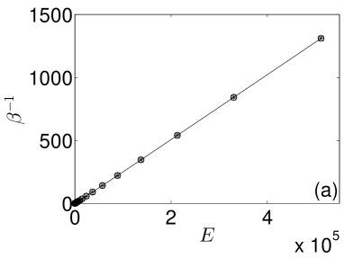
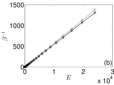
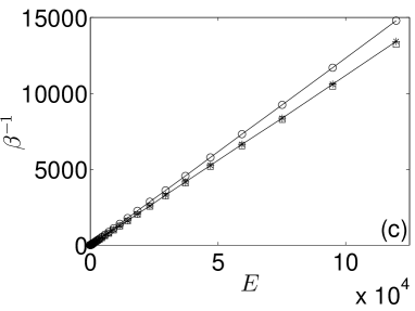
Figure 1: The figure compares the $\beta^{-1}$ derived from the three different definitions (9), (10) and (11) and measured for several values of the total density energy $E$ for different particle numbers: (a) $n=512$, (b) $n=24$, (c) $n=12$. We report the measured values for $\beta_{s}^{-1}$ using stars ($\star$), the measured values for $\beta^{-1}_{et}$ using open squares ($\Box$) and the measured values for $\beta^{-1}_{B}$ using open circles ($\circ$).

In Fig. 1 we report the comparison of the curves $\beta^{-1}(E)$ derived from the three different definitions (9), (10) and (11) and measured for several values of the total density energy $E$ and some system sizes. Already in the case of a system size of $512$ particles, the the inverse temperatures derived from the three entropy definitions agree in an excellent way. Remarkably, also in the case of a very small system size, as in the case reported in Fig. 1 panel (c), the two definitions (10) and (11) have a very good accordance. Nevertheless, the smaller the system size, the higher the discrepancy between $\beta^{-1}_{B}$ and the measured values of $\beta_{s}^{-1}$ and $\beta^{-1}_{et}$.

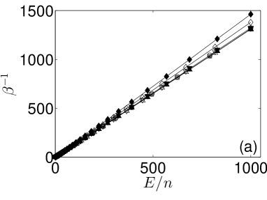
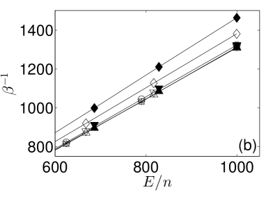
Figure 2: The figure compares the $\beta^{-1}$ derived from the three different definitions (9), (10) and (11) and measured for several values of the total density energy $E/n$ and three system sizes. In panel (a), with stars ($\star$) we report the measured values for $\beta^{-1}_{s}$ in the case $n=128$, with open squares ($\Box$) the measured values for $\beta^{-1}_{et}$ in the case $n=128$ and with open circles ($\circ$) the measured values for $\beta^{-1}_{B}$ in the case $n=128$. With open down triangles ($\triangledown$) we report the measured values for $\beta^{-1}_{s}$ in the case $n=24$, with open up triangles ($\triangle$) the measured values for $\beta^{-1}_{et}$ in the case $n=24$ and with open diamonds ($\lozenge$) the measured values for $\beta^{-1}_{B}$ in the case $n=24$. With full down triangles ($\blacktriangledown$) we report the measured values for $\beta^{-1}_{s}$ in the case $n=12$, with full up triangles ($\blacktriangle$) the measured values for $\beta^{-1}_{et}$ in the case $n=12$ and with full diamonds ($\blacklozenge$) the measured values for $\beta^{-1}_{B}$ in the case $n=12$. Panel (b), is a magnification of a small region of panel (a).

In Fig. 2 panel (a) we compare the curves $\beta^{-1}(E/n)$ derived from the three definitions (9), (10) and (11) and measured for several values of the density of the total energy $E/n$ and for three system sizes. Fig. 2 panel (b) is a magnification of a small region in Fig. 2 (a). Both the figures display the features described above: $\beta^{-1}$ derived according to the two definitions (10) and (11) show a very good accordance one another for large as well as small system size, and the smaller the system size, the higher the deviation between $\beta^{-1}_{B}$ and $\beta_{s}^{-1}$ and $\beta^{-1}_{et}$.

This analysis shows that the thermodynamic quantities derived from Boltzmann entropy in the case of a small system can be affected by relevant deviations from the asymptotic behaviour. On the contrary, the same does not happen when using the surface entropy. This seems to indicate that the microstatistical description of “intrinsically small” systems (nanoparticles, proteins, cellular systems) could be profitably improved by resorting to the surface entropy instead of the Boltzmann entropy.

Furthermore, in our opinion, the deviation of $\beta^{-1}_{B}$ from $\beta^{-1}_{et}$ observed when the system size is decreased can bring to a serious logical issue. In fact, let’s consider a macroscopic isolated system ${\cal S}$ at equilibrium, with a total energy density $\epsilon$, and let $\beta^{-1}_{B}=\beta^{-1}_{et}$ be the temperature of the system. We can now consider a small piece of such a system, ${\cal S}^{\prime}$, which is composed only by few particles. Obviously, the energy density $\epsilon^{\prime}$ of ${\cal S}^{\prime}$ will fluctuate with time. But, we can imagine to isolate the small system from the rest, exactly when the value of its energy density is $\epsilon$. Obviously, in this state, also the energy density of the rest of the system amount to $\epsilon$. We have two isolated (sub)systems, a macroscopic one and a small one. Now, by using the surface entropy, we obtain the same estimation of the temperature for both the systems, ${\cal S}$ and ${\cal S}^{\prime}$. On the contrary, the Boltzmann entropy provides a different estimation for the temperature of the small system.

III Derivation of the surface entropy

We have emphasized that the surface entropy fixes some of the pathologies that the Boltzmann entropy exhibits in the statistical description of small systems. By pushing our reasoning forward, we speculate that the issues shown by the Boltzmann entropy in the statistical description of small systems is actually the signature of a deeper flaw in its definition.

The postulate of equal a-priori probability, for a macroscopic system in thermodynamic equilibrium, asserts that its state is equally likely to be any state satisfying the macroscopic conditions of the system. Now, in the case of the microcanonical ensemble, usually one assumes as macroscopic condition for the system that its energy has values within a small interval of amplitude $\Delta E$ around $E$. Thus, the postulate of equal a-priori probability leads to the probability distribution

$$\rho(x)=\left\{\begin{array}[]{l}constant\,,\quad\mathrm{if}\,E\leq H(x)\leq E+\Delta E\,,\\ 0\,,\quad\mathrm{otherwise}\,.\end{array}\right.$$ (12)

In the limit $\Delta E\to 0$, this density leads to the expression for the measure on the energy-level hypersurfaces

$$\dfrac{m^{N-1}(\Sigma_{E})}{\|\nabla H(x)\|}\,,$$ (13)

whence one obtains the Boltzmann entropy. Nevertheless, if we assume as macroscopic condition for the system that its energy has a fixed value $E$, the postulate of equal a-priori probability leads to the probability distribution for the system

$$\rho(x)=\left\{\begin{array}[]{l}constant\,,\quad\mathrm{if}\,H(x)=E\,,\\ 0\,,\quad\mathrm{otherwise}\,,\end{array}\right.$$ (14)

that is the measure on the energy-level hypersurfaces

$${m^{N-1}(\Sigma_{E})}\,,$$ (15)

whence the surface entropy definition descends. Surface and Boltzmann entropies are inequivalent since the first assumes a uniform probability density on the constant energy hypersurface whereas in the case of the Boltzmann entropy the probability density is $1/\|\nabla H\|$. This entails in the second case a “concentration” of probability near to the points where the norm of the Hamiltonian gradient decreases. This is well shown in the simple example reported in Fig. 3.

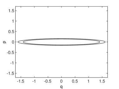
Figure 3: The figure shows two surfaces of constant energy for a one-dimensional harmonic oscillator with Hamiltonian $H=\beta^{2}p^{2}/2+q^{2}/2$. The two ellipses correspond to the choice $\beta=10$ and energy values $E_{1}=1$ (internal) and $E_{2}=1.3$ (external). The area difference is a strip of non-uniform thickness representing the inverse of the gradient norm of $H$, that is the non-uniform density probability of Eq. (13).

From this point of view, the two entropies derive from the two different definitions of isolated system.

For a classical isolated system, one can assume that the value of its total energy does not range in some finite interval of values but has some assigned value. Also within a quantum description, one can always assume an isolated system to be in an eigenstate of the Hamiltonian operator. Moreover, both in the classical and quantum cases, the energy indetermination $\Delta E$ is difficult to be quantified: it should be related to a measure process, that has a restricted meaning in the equilibrium theory. In other words, $\Delta E$ seems not to be a well-defined quantity which one gets rid of in the limit $\Delta E\to 0$ process.

On the other hand, it is important to emphasize the following property of the standard Boltzmann entropy. For the Boltzmann entropy, the measure on phase-space (13) coincides with the microcanonical invariant measure of the Hamiltonian dynamics. This fact has two main consequences: first, the possibility to measure the thermodynamical average of any physical quantity by means of time averages along a trajectory (or with phase-space integrals if the ergodic theorem holds true); second, and more important, the statistical weight of each microscopic configuration is invariant under the Hamiltonian flow. The first point is not an issue. In fact, the thermodynamic quantities, as, for instance, temperature and specific-heat, are defined in term of the derivatives of the entropy with respect to the energy, and in the case of the surface entropy, these derivatives can be measured via microcanonical averages along the dynamics, by using tricks analogous to that used in Eq. (10). As to the second point, the measure (15) is not invariant under the Hamiltonian flux. Nevertheless, $\Sigma_{E}$, its volume, and, consistently, $S_{s}$ are invariant under the Hamiltonian flux. This means that in the case of the surface entropy the invariance under the dynamics is a global property rather than local. The limitation from local to global of the invariance under the Hamiltonian flux that we have in the case of the surface entropy has no physical consequences since it is not experimentally observable. In fact, the thermodynamical quantities of an isolated system at equilibrium depend on the global entropy and not from local quantities. In addition, in order to measure in an experiment a given local property, it is necessary an interaction with an external apparatus and this makes the system no more isolated.

IV Consequences of the surface entropy

From a geometric point of view, the temperature derived from the surface entropy has an interesting interpretation: it is the average of the mean curvature of $\Sigma_{E}$ (the hypersurface $H(x)=E$) which is a geometric quantity. In fact, in Franzosi (2018) we have shown that in the case of the surface entropy it results

$$\beta_{s}=\dfrac{\int_{\Sigma_{E}}M(x)m^{N-1}(\Sigma_{E})}{\int_{\Sigma_{E}}m^{N-1}(\Sigma_{E})}\,,$$ (16)

where

$$M(x)=\dfrac{1}{\|\nabla H\|}\nabla\cdot\left(\dfrac{\nabla H}{\|\nabla H\|}\right)$$ (17)

is the local mean curvature divided by $\|\nabla H\|$. The latter term makes intensive the quantity measured with this average, as it is requested for the inverse temperature.

It is worth noting that it might be necessary to use the surface entropy instead of the usual Boltzmann form, also in the case of macroscopic systems in which the phase-space volume scales up as a function of the number of degrees of freedom of the system slower than exponentially. This is the case of the long-range interactions. In fact, in systems with short-range interaction the measure of the volumes $H(x)\leq E$ concentrates on the hypersurface $H(x)=E$ when the number of the degrees of freedoms increases, whereas for systems with long-range interaction the same is not necessarily true. Therefore, for the latter systems, the differences between the quantities derived using the surface and the Boltzmann entropy can be measurable also up to macroscopic sizes of the system.

A further domain of application of the surface entropy may be the problem of negative specific heats in the microcanonical ensemble Carignano and Gladich (2010). This phenomenon, that seems to violate the laws of thermodynamics, takes place in small systems (absolutely far from the thermodynamic limit), that is in systems with size smaller or comparable to the range of the forces driving their dynamics. For this reason, in these systems the equivalence between canonical and microcanonical ensembles is not valid and the microcanonical approach is the only that explains the emergence of negative specific heat. Examples of systems of this kind are found in different fields: we just mention clusters of sodium atoms Schmidt et al. (2001), clusters of stars Lynden-Bell (1999) and plasma Kiessling and Neukirch (2003).