Branching structures emerging from a continuous optimal transport model

Abstract.

Recently a Dynamic-Monge-Kantorovich formulation of the PDE-based $L^{1}$-optimal transport problem was presented. The model considers a diffusion equation enforcing the balance of the transported masses with a time-varying conductivity that evolves proportionally to the transported flux. In this paper we present an extension of this model that considers a time derivative of the conductivity that grows as a power law of the transport flux with exponent $\beta>0$. A sub-linear growth ($0<\beta<1$) penalizes the flux intensity and promotes distributed transport, with equilibrium solutions that are reminiscent of Congested Transport Problems. On the contrary, a super-linear growth ($\beta>1$) favors flux intensity and promotes concentrated transport, leading to the emergence of steady-state “singular” and “fractal-like” configurations that resemble those of Branched Transport Problems. We derive a numerical discretization of the proposed model that is accurate, efficient, and robust for a wide range of scenarios. For $\beta>1$ the numerical model is able to reproduce highly irregular and fractal-like formations without any a-priory structural assumption.

1. Introduction

In this paper we propose and analyze theoretically and numerically an extension of the Dynamic Monge-Kantorovich (DMK) Optimal Transport (OT) model recently presented in Facca et al. [12]. The DMK can be summarized as follows. Consider an open, bounded, connected, and convex domain $\Omega$ in $\mbox{\NUMBERS R}^{d}$ with smooth boundary. Given two non-negative rate densities, $f^{+}$ and $f^{-}$ such that $\int_{\Omega}f^{+}\,dx=\int_{\Omega}f^{-}\,dx$, consider $f:=f^{+}-f^{-}$. We want to find the pair $(\mu,u):[0,+\infty[\times\Omega\mapsto\mbox{\NUMBERS R}^{+}\times\mbox{\NUMBERS R}$ that solves:

(1a) $$-\operatorname{\operatorname{\nabla\cdot}}\left(\mu(t,x)\operatorname{\nabla}u(t,x)\right)=f(x),$$

(1b) $$\mu^{\prime}(t,x)=\mu(t,x)\left|\operatorname{\nabla}u(t,x)\right|-\mu(t,x),$$

(1c) $$\mu(0,x)=\mu_{0}(x)>0,$$

completed with zero Neumann boundary conditions. Here $\mu^{\prime}$ denotes derivative with respect to time. Hereafter, we omit the dependence from $x$ and kept only the time-dependence. We will use this convention whenever no confusion arises.

In Facca et al. [12] it is conjectured that the solution pair $(\mu(t),u(t))$ as function of time converges for $t\rightarrow\infty$ towards $(\mu^{*},u^{*})$ where, $\mu^{*}$ is the OT density and $u^{*}$ is a Kantorovich Potential associated to $f^{+}$ and $f^{-}$. The pair $(\mu^{*},u^{*})$ solves the Monge-Kantorovich (MK) partial differential equations introduced in Evans and Gangbo [11]. Local existence and uniqueness of $(\mu(t),u(t))$ for $t\in[0,\tau_{0}[$, with $\tau_{0}>0$ depending on the initial data, was proved under the hypotheses that $\mu_{0}$ is Hölder continuous and $f\in L^{\infty}(\Omega)$. However, well posedness and full regularity of the solution, as well as its convergence towards the solution of the MK equations, are still open issues. The conjecture is strongly supported by convincing numerical results reported in Facca et al. [12, 13]. Additionally, a Lyapunov-candidate functional for the dynamics is given by:

$$\mathcal{L}(\mu)=\frac{1}{2}\int_{\Omega}{\mu\left|\operatorname{\nabla}u_{f}(\mu)\right|^{2}}\,dx+\frac{1}{2}\int_{\Omega}{\mu}\,dx,$$

where $u_{f}(\mu)$ indicates the weak solution of the elliptic equation Eq. 1a for a given $f$. It is possible to prove that $\mathcal{L}$ decreases along the $\mu(t)$-trajectory and the OT density is its unique minimizer [13].

The extension we propose in this paper, suggested by the discrete counterpart reported in Tero et al. [22], modifies the dynamics of $\mu(t)$ by introducing a power law of the transport flux $\mu(t)\left|\operatorname{\nabla}u(t)\right|$ with exponent $\beta>0$. The proposed model can be described as the problem of finding the pair $(\mu(t),u(t))$ such that:

(2a) $$-\operatorname{\operatorname{\nabla\cdot}}\left(\mu(t)\operatorname{\nabla}u(t)\right)=f,$$

(2b) $$\mu^{\prime}(t)=\left[\mu(t)\left|\operatorname{\nabla}u(t)\right|\right]^{\beta}-\mu(t),$$

(2c) $$\mu(0)=\mu_{0}(x)>0,$$

completed with zero Neumann boundary conditions. Assuming well-posedness of the above system, we claim that, as in the case $\beta=1$, the solution pair $(\mu(t),u(t))$ converges toward an equilibrium configuration $(\mu^{*},u^{*})$ as $t\rightarrow\infty$. Moreover, we claim that this equilibrium point should be related to congested ($0<\beta<1$) and branched ($\beta>1$) OT problems. In fact, intuitively, a sub-linear growth should penalize flux intensity (i.e. the transport density) and promote distributed transport. Correspondingly, the equilibrium solutions should be reminiscent of Congested Transport Problem (CTP), a branch of OT theory that studies reallocation problems where mass concentration is penalized, and finds applications in, e.g., crowd motion and urban traffic (see, e.g., [21, 7, 9]). On the other hand, a super-linear growth should favor flux intensity and promote concentrated transport, leading to the emergence of “singular” and “fractal-like” configurations that resemble the structures typical of Branched Transport Problem (BTP). Branched transport is an area of OT that studies reallocation problems where mass concentration is encouraged along the transport paths, favoring “economy of scale”. This is a common strategy that can be easily assumed to be a fundamental mechanism in the development of many natural systems such as, e.g., tree branches and roots, blood vessels, river networks, etc. [1, 2, 19]. Note that any homogeneous positive function can replace the power law, thus non-linearly modulating the mixing of the different behaviors. We are interested in the simpler case of the power law as a model problem that incorporates all the interesting responses.

The above claims are supported by extensive numerical experiments on a number of different two-dimensional test cases and by some partial results and heuristic justifications. Among the latter, we are able to derive a Lyapunov-candidate functional $\mathcal{L}_{\beta}$ given by:

(3a) $$\mathcal{L}_{\beta}(\mu):=\mathcal{E}_{f}(\mu)+\mathcal{M}_{\beta}(\mu),$$

(3b) $$\mathcal{E}_{f}(\mu):=\frac{1}{2}\int_{\Omega}{\mu\left|\operatorname{\nabla}u_{f}(\mu)\right|^{2}}\,dx;\qquad\mathcal{M}_{\beta}(\mu):=\begin{cases}\displaystyle\frac{1}{2}\int_{\Omega}\ln(\mu)\,dx&\text{if }\beta=2\\ \displaystyle\frac{1}{2}\int_{\Omega}\frac{\mu^{\frac{2-\beta}{\beta}}}{\frac{2-\beta}{\beta}}\,dx&\text{otherwise}\end{cases}.$$

Similarly to the case $\beta=1$, $\mathcal{L}_{\beta}$ decreases in time along the $\mu(t)$-trajectory, thus it is natural to investigate if the Lyapunov-candidate functional admits a minimum, which is the natural limit candidate for our dynamics. Intuitively, such minimum provides a trade-off between the transport cost, measured by the term $\mathcal{E}_{f}(\mu)$, and the “infrastructure” cost, measured by the term $\mathcal{M}_{\beta}(\mu)$. For $0<\beta\leq 1$ the second term is convex, penalizing the concentration of the support of $\mu$, as prescribed by the CTP. On the other hand, for $1<\beta<2$ $\mathcal{M}_{\beta}(\mu)$ is concave, favoring the concentration of $\mu$ on narrow supports.

For the case $0<\beta<1$, we claim that the pair $(\mu(t),u(t))$ converges at long times toward $(\left|\operatorname{\nabla}u_{p}\right|^{p-2},u_{p})$, with $p=\frac{2-\beta}{1-\beta}$, where $u_{p}$ is the solution of the $p$-Poisson equation with forcing term $f$:

$$-\operatorname{\operatorname{\nabla\cdot}}(\left|\operatorname{\nabla}u_{p}\right|^{p-2}\operatorname{\nabla}u_{p})=f.$$

This conjecture is supported by the fact that, for $q=2-\beta$, minimization of $\mathcal{L}_{\beta}$ is equivalent to the following variational problem:

(4) $$\inf_{v\in[L^{q}(\Omega)]^{d}}\left\{\int_{\Omega}\frac{\left|v\right|^{q}}{q}\,dx\ :\ \operatorname{\operatorname{\nabla\cdot}}(v)=f\right\},$$

that is a classical formulation of the CTP. The equivalence between problem Eq. 4 for $q\in[1,2]$ and the solution of the $p$-Poisson equation, with $p$ conjugate to $q$, is a well known result [10]. The equivalence for $\beta=1,q=1$ has been proved in Facca et al. [12]. Analogously to the case $\beta=1$ studied in [12, 13], this new formulation of the $p$-Poisson equation leads to robust and accurate numerical discretization schemes, providing an unconventional yet very efficient approach, at least with respect to the classical augmented Lagrangian strategy usually adopted for the numerical solution of the $p$-Poisson equation [14, 3, 4].

The case $\beta>1$ is mostly addressed by numerical experimentation. A number of two-dimensional tests suggest a connection between the steady state equilibrium solution $(\mu^{*},u^{*})$ of the proposed model and solutions of the BTP, in particular, our reference formulation is that one introduced by Xia [26]. In this formulation,  Eq. 4 is rewritten in the case $0<q<1$, where the integral must be reinterpreted appropriately. Thus we now look for a vector valued measure $v$ solving for $0<q<1$ the following minization problem

(5) $$\inf_{v\in[\mathcal{M}(\Omega)]^{d}}\left\{\int_{\Omega}\left|\frac{dv}{d\mathcal{H}^{1}}\right|^{q}d\mathcal{H}^{1}\ :\ \operatorname{\operatorname{\nabla\cdot}}(v)=f\,dx\right\},$$

where $d\mathcal{H}^{1}$ denote the Hausdorff measure of dimension 1 (see  [21, 23] for the detailed definition). Although in our case we are still not able to exactly identify the relations with the reference BTP  formal calculations backed up by several numerical results, suggest strong connections with the functionals minimized in more classical BT problems. More precisely, we are not able to rigorously consider the singular measures typically arising in BT transport, but the numerical results are convincingly leading to structures that closely resemble the BT transport solutions.

Notwithstanding some evident numerical inaccuracies in approximating these singular structures and computational difficulties encountered in the solution of the highly ill-posed linear systems arising from the discretization of the elliptic equation, long-time numerical solutions seem to invariably reach a state of equilibrium. Correspondingly, depending on the source term, the spatial distributions of the approximated transport density $\mu_{h}^{*}$ seem to converge to fractal-like or low-dimensional structures. These singular configurations are shown to be sensitive to initial conditions, probably corresponding to local minima of a non-convex Lyapunov-candidate functional, being the sum of a convex and a concave functional, $\mathcal{E}_{f}$ and $\mathcal{M}_{\beta}$ . On the other hand, all the numerical experiments presented in this paper show how the supports of $\mu_{h}^{*}$ have the structure of an acyclic graph connecting the supports of $f^{+}$ and $f^{-}$. The absence of loops is a fundamental characteristic of the solution of the BTP  never imposed a priori in our model, that seems to suggest yet another relationship between the long-time numerical solution of DMK and the BT transport solution.

Only sparse examples in the literature addressing the numerical solution of the BT problem exist, both in the discrete [24] and in the continuous settings [17]. In this last work the authors introduce a $\varepsilon$-relaxed functional $\Gamma$-converging to the minimizer of problem in Eq. 4 as $\varepsilon\to 0$. A conjugate Gradient algorithm combined with finite difference spatial discretizations is used to find sequence of approximated minimizer. This approach has been showed to able to solve the BTP in simple problem settings, but still it suffers of the main problems we are facing in our approach ( e.g., parameters tuning, convergence to local minima).

In conclusion of this introduction, we would like to remark the similarities between the model proposed in our paper and the revisited version of the PP model presented in the discrete setting in [16] and, in a continuous setting, in the model of [15], where the modulating exponent $\beta$ is moved from the flux to the decay term of Eq. 2. In a recent analysis, [8] studies a model that is similar to our proposed dynamics under special conditions and connects it to discrete optimization problems addressing CTP and BTP. Moreover, our work seems to be related to the work in [25] on the discrete $p$-Laplace with $p<0$.

In this paper we want to highlight the optimization capabilities of the model that, despite the above mentioned limitations, seems to be well-suited for the solution of optimal (branched and congested) transport problems without imposing any a-priory graph topology. This is particularly relevant in the case of BTP where the topology of the optimal solution is actually the main unknown. Our results show that the relaxation introduced by the time-dependency in our extended DMK allows a relatively easy numerical formulation that is efficient and robust.

2. Lyapunov-candidate functional and its minimization

The local existence result obtained in [12] could be extended to the case $\beta>1$, but, numerical simulations and theoretical considerations suggest that the assumption of Hölder-continuity of $\mu$ needs to be relaxed. In this case any existence result seem out of reach at this time. However, being mostly concerned with the asymptotic behavior of $(\mu(t),u(t))$ solution of Eq. 2, in this work we assume existence and uniqueness of a solution pair for all $t\geq 0$, and present the formal derivation of the Lyapunov-candidate functional for all $\beta>0$, as given by the following Proposition.

Proposition 1.

Assume that there exists $\bar{t}>0$ such that Eq. 2 admits a solution pair $\left(\mu(t),u(t)\right)$ with $\mathcal{C}^{1}$-regularity in time for $t\in[0,\bar{t}[$. Then the Lyapunov-candidate functional $\mathcal{L}_{\beta}$ given in Eq. 3 is strictly decreasing along the $\mu(t)$ trajectories for all $\beta>0$, and its Lie derivative is given by:

(6) $$\frac{d}{dt}\left(\mathcal{L}_{\beta}(\mu(t))\right)=\\ -\frac{1}{2}\int_{\Omega}{\mu(t)^{\beta}\left(\left|\operatorname{\nabla}u(\mu(t))\right|^{\beta}-\mu^{\left(\frac{1-\beta}{\beta}\right)\beta}(t)\right)\left(\left|\operatorname{\nabla}u(\mu(t))\right|^{2}-\left(\mu^{\frac{1-\beta}{\beta}}(t)\right)^{2}\right)}\,dx.$$

Proof.

The proof is based on the equality

$$\frac{d}{dt}\left(\mathcal{E}_{f}(\mu(t))\right)=-\frac{1}{2}\int_{\Omega}{\mu^{\prime}(t)\left|\operatorname{\nabla}u_{f}(\mu(t))\right|^{2}}\,dx,$$

proved in [12] under the assumption of existence and uniqueness of the solution pair $(\mu(t),u(t))$. As a consequence, we can write:

$$\frac{d}{dt}\left[\mathcal{L}_{\beta}(\mu(t))\right]=\frac{d}{dt}\left[\mathcal{E}_{f}(\mu(t))+\mathcal{M}_{\beta}(\mu(t))\right]=\\ =-\frac{1}{2}\int_{\Omega}{\mu^{\prime}(t)\left(\left|\operatorname{\nabla}u_{f}(\mu(t))\right|^{2}-\mu^{\frac{2-\beta}{\beta}-1}(t)\right)}\,dx.$$

Substituting $\mu^{\prime}(t)$ defined by Eq. 2b in the previous equation, using for simplicity $u(t)$ in place of $u_{f}(\mu(t))$ and rearranging terms, we can write:

$$\frac{d}{dt}\mathcal{L}_{\beta}(\mu(t)) =-\frac{1}{2}\int_{\Omega}{\left(\left(\mu(t)\left|\operatorname{\nabla}u(t)\right|\right)^{\beta}-\mu(t)\right)\left(\left|\operatorname{\nabla}u(t)\right|^{2}-\mu^{\frac{2-\beta}{\beta}-1}(t)\right)}\,dx$$

$$\!=-\frac{1}{2}\int_{\Omega}{\mu(t)^{\beta}\left(\left|\operatorname{\nabla}u(t)\right|^{\beta}-\left(\mu^{\frac{1-\beta}{\beta}}(t)\right)^{\beta}\right)\left(\left|\operatorname{\nabla}u(t)\right|^{2}-\left(\mu^{\frac{1-\beta}{\beta}}(t)\right)^{2}\right)}\,dx,$$

which shows that the derivative of $\mathcal{L}_{\beta}$ along the $\mu(t)$-trajectories is strictly negative, since $\mu(t)$ is always strictly greater than zero when starting from a positive initial condition $\mu_{0}>0$. The same computations holds also for the case $\beta=2$. ∎

From Eq. 6 we can formally deduce that the derivative of $\mathcal{L}_{\beta}$ is equal to zero only when evaluated at the pair $(\mu^{*},u^{*})$ solution of:

(7) $$\left\{\begin{aligned} &-\operatorname{\operatorname{\nabla\cdot}}\left(\mu^{*}\operatorname{\nabla}u^{*}\right)=f,\\ &\mu^{*}=\left|\operatorname{\nabla}u^{*}\right|^{\frac{\beta}{1-\beta}}\quad\text{on}\quad\left\{\mu^{*}>0\right\},\end{aligned}\right.$$

when $\beta\neq 1$. It is worth pointing out that these last equations coincide with those we would obtain by imposing $\mu^{\prime}(t)=0$ in Eq. 2b. Moreover Eq. 7 immediately suggests a link between the large-time equilibrium state of Eq. 2 and the $p$-Poisson equation

$$-\operatorname{\operatorname{\nabla\cdot}}\left(\left|\operatorname{\nabla}u_{p}\right|^{p-2}\operatorname{\nabla}u_{p}\right)=f,$$

if the following relation between the exponents $\beta$ and $p$ holds

$$p-2=\frac{\beta}{1-\beta}.$$

However, since we are not able to provide rigorous proofs for all values of $\beta>0$, we analyze separately the cases $0<\beta<1$ and $\beta>1$, which, as it will be seen later, are related to the Congested and Branched Transport Problems, respectively.

2.1. Case $0<\beta<1$

In this instance we are able to show that the minimum of the Lyapunov-candidate functional $\mathcal{L}_{\beta}$ is related to the solution of a $p$-Poisson equation, as stated in the following Proposition.

Proposition 2.

Let $r=r(\beta)=(2-\beta)/\beta$, $q=q(\beta)=2-\beta$, $0<\beta<1$, $\mathcal{L}_{\beta}$ be defined as in Eq. 3, and $L^{r}_{+}(\Omega)$ be the space of non-negative functions in $L^{r}(\Omega)$. Given $f^{+},f^{-}\in L^{2}(\Omega)$ with equal mass, then

(8) $$\inf_{\mu\in L^{r}_{+}(\Omega)}\mathcal{L}_{\beta}(\mu)=\inf_{v\in[L^{q}(\Omega)]^{d}}\left\{\int_{\Omega}{\frac{\left|v\right|^{q}}{q}}\,dx\ :\ \operatorname{\operatorname{\nabla\cdot}}v=f\right\}.$$

Moreover, the functional $\mathcal{L}_{\beta}$ admits a unique minimizer $\mu_{\beta}^{*}\in L^{r}_{+}(\Omega)$ given by $\mu_{\beta}^{*}=\left|\operatorname{\nabla}u_{p}\right|^{p-2}$ where $u_{p}$ is the weak solution of the $p$-Poisson equation

(9) $$-\operatorname{\operatorname{\nabla\cdot}}(\left|\operatorname{\nabla}u_{p}\right|^{p-2}\operatorname{\nabla}u_{p})=f,$$

with $p$ the conjugate exponent of $q$, i.e., $p=\frac{2-\beta}{1-\beta}$.

Proof.

We start the proof recalling the following variational characterization of the energy functional $\mathcal{E}_{f}$ for a general non-negative measure $\mu$ [6]:

(10) $$\mathcal{E}_{f}(\mu) =\sup_{\varphi\in W^{1,p}(\Omega)}\!\left\{\int_{\Omega}\varphi f\,dx-\int_{\Omega}\frac{\left|\operatorname{\nabla}\varphi\right|^{2}}{2}\mu\,dx\right\}$$

$$=\inf_{w\in[L_{\mu}^{2}(\Omega)]^{d}}\!\left\{\int_{\Omega}\frac{\left|w\right|^{2}}{2}\mu\,dx\,:\,\operatorname{\operatorname{\nabla\cdot}}(\mu w)=f\right\},$$

where $W^{1,p}(\Omega)$ is the classical Sobolev space and, with some abuse of notation, $L_{\mu}^{2}=\{v:\int_{\Omega}v^{2}\mu\,dx<\infty\}$. Note that in the above result the divergence constraint is considered in the sense of distributions. Then, we can rewrite $\mathcal{L}_{\beta}(\mu)$ as:

(11) $$\mathcal{L}_{\beta}(\mu)=\inf_{w\in[L_{\mu}^{2}(\Omega)]^{d}}\left\{\Theta_{\beta}(\mu,w)\ :\operatorname{\operatorname{\nabla\cdot}}(\mu w)=f\right\}\quad\forall\mu\in L^{r(\beta)}_{+}(\Omega),$$

where

$$\Theta_{\beta}(\mu,w):=\frac{1}{2}\int_{\Omega}{\left|w\right|^{2}\mu}\,dx+\frac{1}{2}\int_{\Omega}{\frac{\mu^{\frac{2-\beta}{\beta}}}{\frac{2-\beta}{\beta}}}\,dx.$$

For any pair $(\mu,w)\in\left(L^{r}_{+}(\Omega),[L_{\mu}^{2}(\Omega)]^{d}\right)$ and for $q\in]1,2[$, we use Young inequality with conjugate exponents $2/q$ to obtain:

$$\int_{\Omega}{\left|w\mu\right|^{q}}\,dx=\int_{\Omega}{\left|w\right|^{q}\mu^{q/2}\mu^{q/2}}\,dx\leq\frac{q}{2}\int_{\Omega}{\left|w\right|^{2}\mu}\,dx+\frac{2-q}{2}\int_{\Omega}{(\mu^{\frac{q}{2}})^{\frac{2}{2-q}}}\,dx.$$

Since $\frac{q}{2-q}=\frac{2-\beta}{\beta}$, which yields the relation $q=q(\beta)=2-\beta$, dividing by $q$ we can rewrite the previous inequality as:

(12) $$\int_{\Omega}{\frac{\left|w\mu\right|^{(2-\beta)}}{(2-\beta)}}\,dx\leq\frac{1}{2}\int_{\Omega}{\left|w\right|^{2}\mu}\,dx+\frac{1}{2}\int_{\Omega}{\frac{\mu^{\frac{2-\beta}{\beta}}}{\frac{2-\beta}{\beta}}}\,dx=\Theta_{\beta}(\mu,w),$$

which holds for all $\mu\in L^{r(\beta)}_{+}(\Omega)$ and all $w\in[L_{\mu}^{2}(\Omega)]^{d}$. Now we take the infimum on both sides of the previous equation over the $\mu$-divergence constrained $w\in[L_{\mu}^{2}(\Omega)]^{d}$ and use characterization Eq. 11 to obtain:

$$\inf_{w\in[L_{\mu}^{2}(\Omega)]^{d}}\left\{\int_{\Omega}{\frac{\left|w\mu\right|^{(2-\beta)}}{(2-\beta)}}\,dx\ :\operatorname{\operatorname{\nabla\cdot}}(\mu w)=f\right\}\leq\mathcal{L}_{\beta}(\mu)\quad\forall\mu\in L^{r(\beta)}_{+}(\Omega).$$

Taking the infimum over all $\mu\in L^{r(\beta)}_{+}(\Omega)$ yields:

(13) $$\inf_{\mu\in L^{r(\beta)}_{+}(\Omega)}\left\{\inf_{w\in[L_{\mu}^{2}(\Omega)]^{d}}\left[\int_{\Omega}{\frac{\left|w\mu\right|^{(2-\beta)}}{(2-\beta)}}\,dx\ :\operatorname{\operatorname{\nabla\cdot}}(\mu w)=f\right]\right\}\leq\inf_{\mu\in L^{r(\beta)}_{+}(\Omega)}\mathcal{L}_{\beta}(\mu).$$

According to the relationship between the solution of the $p$-Poisson equation and CTP  we have that for any $q>1$ the optimal vector field is given by [10, ex. 2.2, Chapter 4]:

$$\operatornamewithlimits{argmin\vphantom{q}}_{v\in[L^{q}(\Omega)]^{d}}\left\{\int_{\Omega}{\frac{\left|v\right|^{q}}{q}}\,dx\ :\operatorname{\operatorname{\nabla\cdot}}(v)=f\right\}=v^{*}=-\left|\operatorname{\nabla}u_{p}\right|^{p-2}\operatorname{\nabla}u_{p},$$

where $p$ is the conjugate exponent of $q$. Now, for $q=2-\beta$ (and thus $p=(2-\beta)/(1-\beta)$) and using Eq. 13), we obtain:

(14) $$\int_{\Omega}{\frac{\left|\operatorname{\nabla}u_{p}\right|^{p}}{2-\beta}}\,dx =\int_{\Omega}{\frac{\left|v^{*}\right|^{(2-\beta)}}{2-\beta}}\,dx=\!\!\!\inf_{v\in[L^{(2-\beta)}(\Omega)]^{d}}\left\{\int_{\Omega}{\frac{\left|v\right|^{(2-\beta)}}{2-\beta}}\,dx\ :\operatorname{\operatorname{\nabla\cdot}}(v)=f\right\}$$

$$\leq\inf_{\mu\in L^{r(\beta)}_{+}(\Omega)}\left\{\inf_{w\in[L_{\mu}^{2}(\Omega)]^{d}}\left\{\int_{\Omega}{\frac{\left|w\mu\right|^{(2-\beta)}}{2-\beta}}\,dx\ :\operatorname{\operatorname{\nabla\cdot}}(\mu w)=f\right\}\right\}$$

$$\leq\inf_{\mu\in L^{r(\beta)}_{+}(\Omega)}\mathcal{L}_{\beta}(\mu)\leq\mathcal{L}(\mu^{*}_{\beta})=\mathcal{E}_{f}(\mu^{*}_{\beta})+\mathcal{M}_{\beta}(\mu^{*}_{\beta}).$$

We can compute the term $\mathcal{E}_{f}(\mu^{*}_{\beta})$ as follows. By Eq. 10, the following chain of inequalities is obtained:

$$\int_{\Omega}{\left(fu_{p}-\mu^{*}_{\beta}\frac{\left|\operatorname{\nabla}u_{p}\right|^{2}}{2}\right)}\,dx\leq\sup_{\varphi\in W^{1,p}(\Omega)}\int_{\Omega}{\left(f\varphi-\mu^{*}_{\beta}\frac{\left|\operatorname{\nabla}\varphi\right|^{2}}{2}\right)}\,dx$$

$$=\mathcal{E}_{f}(\mu^{*}_{\beta})=\inf_{w\in[L_{\mu^{*}_{\beta}}^{2}(\Omega)]^{d}}\left\{\int_{\Omega}{\frac{\left|w\right|^{2}}{2}\mu^{*}_{\beta}}\,dx\ :\operatorname{\operatorname{\nabla\cdot}}(\mu^{*}_{\beta}w)=f\right\}\leq\int_{\Omega}{\mu^{*}_{\beta}\frac{\left|\operatorname{\nabla}u_{p}\right|^{2}}{2}}\,dx,$$

Noting that $\int_{\Omega}{fu_{p}}\,dx=\int_{\Omega}{\left|\operatorname{\nabla}u_{p}\right|^{p}}\,dx$ holds since $u_{p}$ is the weak solution of Eq. 9, using $\mu^{*}_{\beta}=\left|\operatorname{\nabla}u_{p}\right|^{p-2}$, we obtain $\mathcal{E}_{f}(\mu^{*}_{\beta})=\int_{\Omega}{\frac{\left|\operatorname{\nabla}u_{p}\right|^{p}}{2}}\,dx$. Using this equality in Eq. 14 and noting that $p=(p-2)(2-\beta)/\beta$, we obtain:

$$\mathcal{L}_{\beta}(\mu^{*}_{\beta})=\mathcal{E}_{f}(\mu^{*}_{\beta})+\mathcal{M}_{\beta}(\mu^{*}_{\beta})=\int_{\Omega}{\frac{\left|\operatorname{\nabla}u_{p}\right|^{p}}{2-\beta}}\,dx.$$

Thus, all the inequalities in Eq. 14 are actually equalities, and we can conclude that $\mu^{*}_{\beta}$ is a minimum, which is unique since the functional $\mathcal{L}_{\beta}$ is strictly convex. This last assertion follows from the observation that $\mathcal{E}_{f}$ is convex, being the supremum of functionals that are linear with respect to $\mu$, and $\mathcal{M}_{\beta}$ is strictly convex for $0<\beta<1$. ∎

Remark 1.

The assumption $f^{+},f^{-}\in L^{2}(\Omega)$ can be relaxed whenever $\int_{\Omega}f\varphi\,dx$ is well defined for all $\varphi\in W^{1,p}(\Omega)$.

Propositions 1 and 2 suggest the formulation of the following conjecture for the case $0<\beta<1$:

Conjecture 1.

For $0\leq\beta\leq 1$ and for any initial data $\mu_{0}$, the pair $(\mu(t),u(t))$, solution of the extended dynamic Monge-Kantorovich equations Eq. 2, converges to the pair $(\left|\operatorname{\nabla}u_{p}\right|^{p-2},u_{p})$, where $u_{p}$ is the solution of the $p$-Poisson equation with

(15) $$p=\frac{2-\beta}{1-\beta}.$$

Remark 2.

We want to emphasize two remarkable facts regarding Conjecture 1. For $\beta\rightarrow 1$ the exponent of the $p$-Laplacian tends to infinity ($p\rightarrow+\infty$), coherently with the fact that the MK equations are the limit of the $p$-Poisson problem, as already shown, e.g., in [11]. At the same time, the exponent $q=2-\beta$ tends to $1$, in agreement with the equivalence between the MK equations and Beckmann Problem. When $\beta\rightarrow 0$ then $\mu(t)\rightarrow 1$ and $u(t)$ converges to the solution of a classical Poisson problem ($p=2$). Thus it is possible to include also the value $\beta=0$ in Conjecture 1,

2.2. Case $\beta>1$

In this section we discuss our attempts to extend the arguments presented in the previous section to the BT problem. We are particularly interested in understanding if the functional $\mathcal{L}_{\beta}(\mu(t))$, which by Proposition 1 is decreasing in time, admits a minimum as $t\rightarrow\infty$ and that this minimum is actually attained at $\mu^{*}$. However, in this case the Lyapunov-candidate functional is strongly non-convex, suggesting that several local minima exist, as indicated also by the numerical results reported in the next section that show strong dependence upon the initial data $\mu_{0}$. Mostly formal calculations and several numerical experiments consistently point towards the existence of a strong connection between BTP and the proposed formulation, but we are not able to exactly identify the BTP equivalent to the minimization of $\mathcal{L}_{\beta}$. In fact, the first part of the proof of Proposition 2 remains valid, at least for the case $1<\beta<2$, in which the exponent $q$ remains positive. Indeed, from Eq. 14 the following sequence of inequalities is derived:

$$\inf_{v\in[L^{q}(\Omega)]^{d}} \left\{\int_{\Omega}{\frac{\left|v\right|^{q}}{q}}\,dx\ :\operatorname{\operatorname{\nabla\cdot}}(v)=f\right\}$$

$$\leq \inf_{\mu,w}\left\{\int_{\Omega}{\frac{\left|w\mu\right|^{q}}{q}}\,dx\ :(\mu,w)\in L^{\frac{2-\beta}{\beta}}_{+}(\Omega)\times[L_{\mu}^{2}(\Omega)]^{d},\quad\operatorname{\operatorname{\nabla\cdot}}(w\mu)=f\right\}$$

$$\leq \inf_{\mu\in L^{r(\beta)}_{+}(\Omega)}\mathcal{L}_{\beta}(\mu).$$

This optimization problem resembles the BTP formulation in Eq. 5. However, we have to highlight an important difference between the two problems. The formulation in [23] uses integrals computed with respect to a Hausdorff measure that well adapts to the singular structures arising in BT. Our computations, on the other hand, are made always with respect to the Lebesgue measure, indicating that relation $q=2-\beta$ does not hold. Moreover, for $\beta\geq 2$, $\mathcal{L}_{\beta}$ is not well defined for $\mu$ attaining zero on some regions of $\Omega$, while we expect that the asymptotic $\mu^{*}$ will be zero on large portions of the domain. These two elements suggest that a proper re-formulation of the Lyapunov-candidate functional is required for $\beta>1$. One possible strategy to reconcile our inability to address singular measures is inspired by the Modica-Mortola approach, effectively used in [20, 17]. The main idea is to introduce a parameter $\varepsilon>0$ in Eq. 12 and use Young inequality with $\varepsilon$ as parameter in order to weight differently the energy and mass terms, $\mathcal{E}_{f}(\mu)$ and $\mathcal{M}_{\beta}(\mu)$, in $\mathcal{L}_{\beta}(\mu)$. Intuitively, $\varepsilon$ should be raised to a suitable power that allows the different energy and mass components to scale correctly. The main difficulty lies in the identification of the proper scaling power, but this identification is at the moment still elusive.

Despite these difficulties, together with some not completely understood theoretical issues, we present in the next section numerical simulations that suggest that system Eq. 2 admits a steady state equilibrium $(\mu^{*},u^{*})$, where the supports of the numerical solutions $\mu_{h}^{*}$ seem to approximate the typically singular (low-dimensional) formations emerging in BT problems and the vector field $v^{*}=-\mu^{*}\operatorname{\nabla}u^{*}$ solve the BTP as formulated in [23].

3. Numerical solution of the Extended DMK equations

In this section we report several two-dimensional numerical tests in support of our conjectures. In particular we try to approximate explicitly the steady state solution of Eq. 2 and look at the qualitative behavior of the equilibrium configurations for $t\rightarrow+\infty$ in the CTP ($0<\beta<1$) and BTP ($\beta>1$) cases. For $0<\beta<1$ we test Conjecture 1 comparing our results with an exact solution $u_{p}$ of the $p$-Poisson equation. For the case $\beta>1$, several experiments point to the existence of a connection between the large-time solution of our model and BTP solutions. For different values of $\beta$ and varying types of source terms $f^{+}$ and $f^{-}$, including two largely different test cases employing distributed and a point sources, our dynamics invariably converges to an equilibrium point in correspondence of which $\mu$ always displays branching singular structures.

3.1. The Numerical Approach

The discretization method is based on the Finite Element approach described in [12, 13]. Eq. 2b is projected into a piecewise constant finite dimensional space defined on a triangulation $\mathcal{T}_{h}(\Omega)$ of the domain $\Omega\subset\mbox{\NUMBERS R}^{d}$. The elliptic equation in Eq. 2a is discretized using linear conforming Galerkin finite elements defined on a mesh $\mathcal{T}_{h/2}(\Omega)$ obtained by uniform refinement of $\mathcal{T}_{h}(\Omega)$ (approach called $\mathcal{P}_{1,h/2}-\mathcal{P}_{0,h}$). We choose this spatial discretization method for its robustness and stability as shown in [13]. Accordingly, the approximate pair $(\mu_{h},u_{h})$ can be written as:

$$u_{h}(t,x)=\sum_{i=1}^{N}u_{i}(t)\varphi_{i}(x)\quad\varphi_{i}\in\mathcal{P}_{1}(\mathcal{T}_{h/2}),$$

$$\mu_{h}(t,x)=\sum_{k=1}^{M}\mu_{k}(t)\psi_{k}(x)\quad\psi_{k}\in\mathcal{P}_{0}(\mathcal{T}_{h}),$$

where $\mathcal{P}_{1}(\mathcal{T}_{h/2})$ and $\mathcal{P}_{0}(\mathcal{T}_{h})$ are piecewise linear conforming and piecewise constant FEM spaces, respectively. The time discretization of the projected system is obtained by means of forward Euler time stepping. Denoting with $\boldsymbol{\mu}^{k}$ and $\boldsymbol{u}^{k}$ the vectors collecting the values of $\mu_{h}$ on the triangles and of $u_{h}$ on the nodes at the $k$-th time step, the following sequence of linear systems needs to be solved:

(16a) $$\boldsymbol{A}[\boldsymbol{\mu}^{k}]\boldsymbol{u}^{k}=\boldsymbol{b},$$

(16b) $$\boldsymbol{\mu}^{k+1}=\boldsymbol{\mu}^{k}+\Delta t_{k}\left[\boldsymbol{B}_{\beta}[\boldsymbol{u}^{k}]\left(\boldsymbol{\mu}^{k}\right)^{\beta}-\boldsymbol{\mu}^{k}\right],$$

where $\boldsymbol{A}[\boldsymbol{\mu}^{k}]$ is the stiffness matrix associated to $\boldsymbol{\mu}^{k}$ and $\boldsymbol{B}_{\beta}[\boldsymbol{u}^{k}]$ is the matrix defining the norm of the gradient of $u_{h}(t^{k},x)$ raised to the power $\beta$. The time stepping is initiated from $\boldsymbol{\mu}^{0}$ obtained by projecting the initial data $\mu_{0}$ on the $\mathcal{P}_{0}(\mathcal{T}_{h})$ space. The above system is then iterated until the norm of the relative variation between two consecutive $\mu_{h}$ solutions is smaller than the tolerance $\tau_{\mbox{{\scriptsize T}}}$, i.e.:

$$\operatorname{var}(\mu_{h}^{k}):=\frac{\left\|\mu_{h}^{k+1}-\mu_{h}^{k}\right\|_{L^{2}(\Omega)}}{\Delta t_{k}\left\|\mu_{h}^{k}\right\|_{L^{2}(\Omega)}})\leq\tau_{\mbox{{\scriptsize T}}}.$$

When this occurs we assume that the equilibrium configuration has been reached.

At each time step, the linear system in Eq. 16a is solved via Preconditioned Conjugate Gradient (PCG) with an ad-hoc preconditioning strategy. This preconditioner, developed and discussed in details in [5], exploits the time-stepping sequence to devise an efficient and robust deflation strategy, whereby partial eigenpairs are evaluated to improve the spectral properties of the preconditioned linear system. This approach is fundamental to achieve convergence of the iterations in particular for the case $\beta>1$.

Remark 3.

It is natural to impose a lower bound on $\mu_{h}$ (say $10^{-10}$) to bound from below the smallest eigenvalue of the stiffness matrix in the FEM formulation and limit its condition number. This was indeed our first attempt. However, we quickly realized that our approach is not influenced by this lower bound. In fact, the solution of the linear system at each time step is the same and requires exactly the same number of PCG iterations irrespectively of the presence of the lower bound. Also the dynamics of $\mu_{h}$ and of the corresponding $\mathcal{L}_{\beta}$ for $0<\beta<2$ are not affected by the lower bound. On the other hand, in the case $\beta\geq 2$, the lower bound influences the value of the Lyapunov-candidate functional  which tends to $-\infty$ as $\mu\rightarrow 0$.

3.2. Numerical Experiments

3.2.1. Case $0<\beta\leq 1$

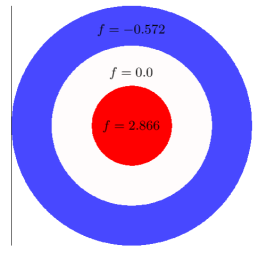
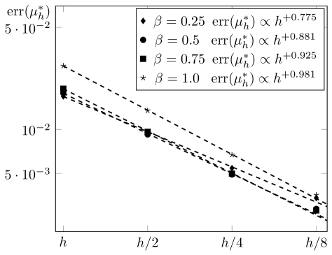
Figure 1. Left panel: spatial distribution of the forcing term $f(x,y)=F(r)$. The mesh points lie on the concentric circles that form the boundary of the supports of $f^{+}$ and $f^{-}$. Center panel: the spatial distribution of $f^{+}$ and $f^{-}$. Right panel: FEM experimental convergence for $\beta=0.25,0.5,0.75,1.0$. The legend above the figure reports the experimental convergence rates for each value of $\beta$.

In this series of tests we compare the long-time limit of $\mu_{h}$, denoted with $\mu_{h}^{*}$, against $\mu_{\beta}^{*}:=\left|\operatorname{\nabla}u_{p}\right|^{p-2}$, where $u_{p}$ is the solution of the $p$-Poisson equation, for which an explicit formula is known, and $p=(2-\beta)/(1-\beta)$, as given by Eq. 15 of Conjecture 1. We consider a two dimensional example taken from [3], where the radially symmetric forcing term is given by $f(x,y)=F(r)$ with $r=\sqrt{x^{2}+y^{2}}$ and $F:]0,1[\mapsto\mbox{\NUMBERS R}$. Under these assumptions, the exact solution of the $p$-Poisson equation is:

$$u_{p}(x,y)=U(r)=-\int_{r}^{1}\operatorname{\operatorname{sign}}(Z(t))\left|Z(t)\right|^{\frac{1}{p-1}}dt\quad Z(r)=-\frac{1}{r}\int_{0}^{r}tF(t)dt.$$

According to the relation between $p$ and $\beta$, we can write the following explicit formula for $\mu^{*}_{\beta}$:

(17) $$\mu^{*}_{\beta}(x,y)=\left|Z(r)\right|^{\frac{p-2}{p-1}}=\left|Z(r)\right|^{\beta}$$

Note that this $\mu^{*}_{\beta}$ is well defined also for $\beta=1$, a value corresponding to the case $p=+\infty$. This optimal density corresponds to the $OT$-density solution of the MK equations, a problem already considered within our setting in Facca et al. [12, 13].

In our numerical experiments we take $F$ as a piecewise constant function, positive in the interval $]0,1/3[$, zero in $[1/3,2/3]$, and negative in $]2/3,1[$. The value of $F$ on the positive and the negative parts is given by two constants $c_{1}$ and $c_{2}$ that are calculated to maintain orthogonality (up to machine precision) of the right hand side $\boldsymbol{b}$ of the linear system Eq. 16a with respect to the constant vectors. This tuning corrects for quadrature errors and is necessary to provide accurate approximations of the integrals and a-priori exclude errors and inaccuracies introduced by the piecewise representations of the circles. The mesh $\mathcal{T}_{h}$ and the forcing term $f$ are shown in Figure 1.

The numerical experiments consist in testing the existence of a steady state $\mu_{h}^{*}$ for different values of $\beta$ (0.25, 0.5, 0.75, 1.0) and evaluating the error with respect to the candidate exact solution $\operatorname{err}(\mu):={\left\|\mu-\mu^{*}_{\beta}\right\|_{L^{2}(\Omega)}}/{\left\|\mu^{*}_{\beta}\right\|_{L^{2}(\Omega)}}.$ We solve the extended DMK equations on a sequence of uniformly refined grids and evaluate the experimental convergence rate by means of $\operatorname{err}(\mu_{h}^{*})$. The sequence is built by uniform refinement of the initial unstructured mesh $\mathcal{T}_{h}(\Omega)$ , characterized by 5191 nodes and 10179 triangles (we generate it using Python package Meshpy). Convergence in time is tested by looking at the evolution of $\operatorname{var}(\mu_{h}(t))$ and $\operatorname{err}(\mu_{h}(t))$. Steady-state is considered achieved when $\tau_{\mbox{{\scriptsize T}}}=5\times 10^{-7}$.

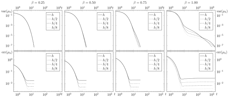
Figure 2. Log-log plots of $\operatorname{var}(\mu_{h}(t,\cdot))$ (upper panels) and $\operatorname{err}(\mu_{h}(t,\cdot))$ (lower panels) vs. time. The columns refer, from left to right, to the results obtained with $\beta=0.25,0.5,0.75,1.0$.

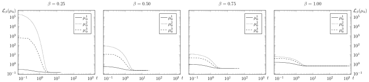
Figure 3. Time behavior of the Lyapunov-candidate functional $\mathcal{L}_{\beta}(\mu_{h}(t)$, for $\beta=0.25,0.5,0.75,1.0$ (from left to right) starting from three different initial data $\mu_{0}$. We report the results only for the coarser mesh as they do not seem to depend on mesh resolution.

The experimental convergence rates are shown in Figure 1, right panel, and vary in the range $m=0.775\div 0.981$ for $\beta=0.25\div 1$, respectively, thus displaying optimal convergence of the spatial discretization. Figure 2 shows the log-log plot of the time-variation $\operatorname{var}(\mu_{h}(t))$ (top row) and the relative error $\operatorname{err}(\mu_{h}(t))$ (bottom row) as a function of time for the same values of $\beta$. From the first set of plots we can see that, as time increases, the variation tends towards zero as power-law with a rate that is independent of the mesh level and decreases as the power $\beta$ increases. In other words, for any tested mesh, the smaller $\beta$ the faster the equilibrium configuration is reached. The case $\beta=1$ shows the slowest convergence towards steady-state and some influence of the mesh resolution appears. This is an evident signal of the difficulty of the MK problem. The relative error (Figure 2, lower row) stagnates at a relatively small time reaching values that decrease at a constant factor with the mesh level, coherently with the experimental convergence rates previously calculated. Note that, for all practical purposes, the time tolerance $\tau_{\mbox{{\scriptsize T}}}$ could be increased to much bigger values without affecting the $\operatorname{err}(\mu_{h}^{*})$, quantity that remains essentially stationary in all simulations after $t=10$, i.e., when $\operatorname{var}(\mu_{h}(t)\in[10^{-3},10^{-4}]$. However, for reasons of numerical testing, all our simulations are continued until the indicated tolerance $\tau_{\mbox{{\scriptsize T}}}$ is achieved.

To conclude our exploration of this case, we look at the time evolution of the Lyapunov-candidate functional $\mathcal{L}_{\beta}(\mu_{h}(t))$ starting from three different initial data $\boldsymbol{\mu}^{0}_{i}\ (i=1,2,3)$. Figure 3 shows the numerical results obtained for the uniform initial condition $\boldsymbol{\mu}^{0}_{1}=1$ and for the $\boldsymbol{\mu}^{0}_{2,3}$ distributions reported later in the left panel of Figure 9. In all simulations $\mathcal{L}_{\beta}(\mu_{h}(t))$ decreases monotonically and always attains the same minimum value independently of the initial conditions. For all the starting points, the value of $\mathcal{L}_{\beta}(\mu_{h}(t))$ becomes numerically stationary before $t=10$. However, its value continues to decrease but at progressively lower rates. Overall, these results provide convincing support of the correctness of Conjecture 1.

3.2.2. Case $\beta>1$

In this section we discuss our numerical results related to ramified transport by looking at some qualitative features that the solutions emerging from our proposed model share with more classical BT solutions reported e.g. in Xia [26]. We explore the numerical features of the discretization algorithm and its robustness by varying the exponent $\beta$, the mesh size parameter $h$, and the initial conditions $\boldsymbol{\mu}^{0}$. We look at the time-convergence of the solution towards an equilibrium point and at the behavior of the Lyapunov-candidate functional $\mathcal{L}_{\beta}$ as $t\rightarrow\infty$. All these results are critically assessed and are here submitted in support of our conjecture on the connection between the asymptotic configuration of our dynamics and the solution of the BTP.

To this aim, we consider three different test cases, TC1, TC2, and TC3 defined on the same domain $\Omega=[0,1]\times[0,1]$ and characterized by varying the forcing function. In TC1, $f^{+}$ and $f^{-}$ are two constant functions with equal value and supports in the rectangular areas $[1/8,3/8]\times[1/4,3/4]$ and $[5/8,7/8]\times[1/4,3/4]$, respectively. TC2 considers $f^{+}$ formed by $50$ Dirac source points randomly distributed in the region $\Omega=[0.1,0.9]\times[0.1,0.9]$, while the sink term $f^{-}$ is a single Dirac mass located at $(0.05,0.05)$ with intensity that balances $f^{+}$. TC3 simulates one Dirac source transporting towards two Dirac sinks, yielding $f^{+}=\delta_{(0.5,0.1)}$) and $f^{-}=0.5\delta_{(0.4,0.9)}+0.5\delta_{(0.6,0.9)}$. For this last case, the exact solution of  Eq. 5 is known as a function of the exponent $q$ and will be considered as reference solution. However, as already noticed in Section 2.2, we do not possess the exact relationship between the exponent $\beta$ of our DMK approach and $q$ of the standard BT formulation, and thus only a qualitative comparison is meaningful.

Sensitivity to initial data is tested for all three TCs by employing the same $\boldsymbol{\mu}^{0}_{i}\ (i=1,2,3)$ used in the previous example. In addition, for TC3, we use initial data concentrated along the reference solution to verify that the dynamics will not move the solution away from a “true” initial guess. We report the results for different values of $\beta\in\{1.1,1.5,2.0,3.0\}$. In this case of ramified transport, we expect $\mu_{h}^{*}$ to concentrate on supports that tend to become progressively singular with respect to the Lebesgue measure as the mesh is refined. Intuitively, the numerical transport density should tend towards zero outside these supports, while it remains positive and may grow indefinitely within these singular sets. This behavior is magnified as $\beta$ grows. Correspondingly, the ill-conditioning of the linear system in Eq. 16a grows, signaled by the large increase of the condition number of the system matrix $\boldsymbol{A}$ well beyond the possibilities of current linear system solvers. This phenomenon is intensified as $\beta$ increases. For this reason we do not address values of $\beta$ larger than 3. For the considered simulations, convergence of the conjugate gradient method is achieved only when using the ad-hoc preconditioner based on spectral information quickly described at the end of Section 3.1, developed and thoroughly tested in [5].

We experimentally test the numerical spatial convergence of the simulator by solving the same problem on successive refinements of an initial triangulation $\mathcal{T}_{h}$. For TC1 we use an initial grid of $1615$ nodes and $3100$ triangles, aligned with the supports of $f^{+}$ and $f^{-}$, while for TC2 the initial mesh is characterized by $1661$ nodes and $3192$ triangles. The $51$ points where the $f$ is concentrated coincide with grid nodes. Again, for all practical purposes, the value $\tau_{\mbox{{\scriptsize T}}}=5\times 10^{-7}$ is more than enough to reach the equilibrium configuration. We discuss the numerical behavior of the model by running simulations with $\beta=1.5$ as a representative example. We look at convergence towards equilibrium, spatial experimental convergence, behavior of the Lyapunov-candidate functional, and sensitivity to initial conditions. For all these tests, the behavior of the numerical solution and the convergence properties of the discretization approach are similar also for the other tested values of $\beta$. In all the numerical simulations, we experimented strong and sudden variations of $\mu_{h}$, since the term $\Delta\mu_{h}^{k}=\boldsymbol{B}_{\beta}[\boldsymbol{u}^{k}]\left(\boldsymbol{\mu}^{k}\right)^{\beta}-\boldsymbol{\mu}^{k}$ in Eq. 16b can rapidly increase by several orders of magnitude. This effect is amplified for larger values of $\beta$. To preserve the stability of the forward Euler scheme we use a time step $\Delta t_{k}$ whose size is tuned according to term $\Delta\mu_{h}^{k}$.

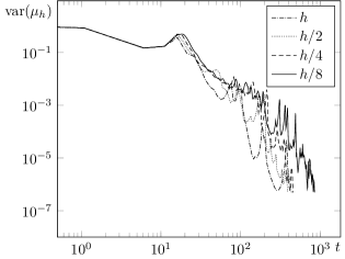
Figure 4. Case $\beta=1.5$, $\boldsymbol{\mu}^{0}\equiv 1$. Time evolution of $\operatorname{var}(\mu_{h}(t))$ on successive mesh refinements for TC1 (left) and TC2 (right).

Convergence towards equilibrium

We first start our discussion by looking at the time evolution of $\operatorname{var}(\mu_{h}(t))$ with uniform initial data $\boldsymbol{\mu}^{0}\equiv 1$ for both TC1 and TC2 (Figure 4). The behavior is globally decreasing but not monotone, unlike the case $\beta\leq 1$. After a reasonably smooth initial transient, the time evolution of $\operatorname{var}(\mu_{h}(t))$ presents oscillations with a frequency that increases at increasing refinement levels. Despite this irregular behavior, in both TCs all simulations seem to converge towards an equilibrium configuration $\left(\mu_{h}^{*},u_{h}^{*}\right)$ for all values of $\beta$ and for every grid and initial data $\boldsymbol{\mu}^{0}$ considered, thus supporting our conjecture that the proposed dynamics converge towards a steady state.

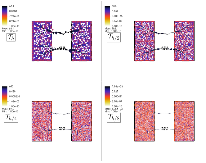
Figure 5. TC1: Numerical approximation $\mu_{h}^{*}$ for $\beta=1.5$ and $\boldsymbol{\mu}^{0}=1$ (logarithmic color scale). The supports of $f^{+}$ and $f^{-}$ are contoured in black. Four successive mesh levels are shown. The dotted rectangle in the lower central channel indicate the zoom window displayed in Figure 7. The color scale is limited at the minimum threshold of $10^{-10}$.

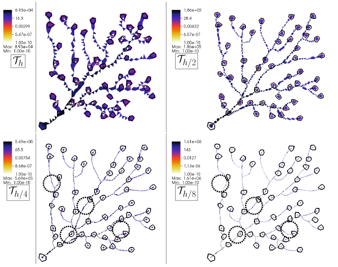
Figure 6. TC2: Numerical approximation $\mu_{h}^{*}$ for $\beta=1.5$ (logarithmic color scale). The initial data $\boldsymbol{\mu}^{0}$ is uniformly equal to $1$ on the entire domain. The small black circles indicate the approximate position of the Dirac masses. Four successive mesh-refinement levels are shown. In the bottom panels we have indicated with dashed circles the location of topological changes between two successively refined network structures. The color scale is limited at the minimum threshold of $10^{-10}$.

The spatial distributions of the limit equilibrium configurations $\mu_{h}^{*}$ are shown in Figures 5 and 6 for $\beta=1.5$ and $\boldsymbol{\mu}^{0}\equiv 1$ at successive grid refinements. Looking at the transient (not shown here), we observe supports of $\mu_{h}$, defined as the union of all triangles in $\mathcal{T}_{h}$ where $\mu_{h}$ is above a minimal threshold of $10^{-10}$, that initially coincide with $\Omega$ but then, as time progresses, tend to create singular structures where $\mu_{h}^{*}$ self-organizes in narrow channels connecting the supports of $f^{+}$ and $f^{-}$. These emerging networks present a hierarchical structure in which channels with higher flow capacity, determined by the values of $\mu_{h}^{*}$, repetitively branch into sub-channels until the whole support of $f$ is covered. The connection between disjoint $f$ supports is ensured by the formation of a limited number of concentrated channels. These emerging structures seem to approach a singular (one-dimensional) tree-like network, where loops are absent.

Notwithstanding the evident difficulty of comparing $\mu_{h}^{*}$ at different refinement levels, an underlying limit network is clearly appearing for all tested values of $\beta$, grid level, or initial data $\boldsymbol{\mu}^{0}$. In particular for TC1, we see in Figure 5 that, inside the supports of $f$, $\mu_{h}^{*}$ forms branching structures with seemingly fractal features. In the region outside the supports of $f$, $\mu_{h}^{*}$ concentrates on a series of connected triangles that create a tight channel with high conductivity linking the source and the sink regions. These effects persists at each refinement level, and the support of $\mu_{h}^{*}$ seems to approximate a one-dimensional network. In TC2 we clearly perceive another phenomenon whereby several branches in the $\mu_{h}^{*}$ tree depart from the expected rectilinear behavior. We attribute this occurrence to a problem of mesh-alignment of the numerical solution, presumably to be ascribed to the extreme spatial irregularity of $\mu_{h}^{*}$. We will discuss this difficulty later on. However, we are positively surprised by the capabilities of our numerical scheme to reproduce, albeit with inaccuracies, these singular structures. A final remark on the emerging structure concerns the occurrence of topological changes between the singular $\mu_{h}^{*}$ spatial distributions at different mesh refinement levels. This is mostly apparent in TC2, where we have highlighted with dotted circles substantial changes in the network topology as $h$ decreases. This phenomenon is an indication of the sensitivity to initial conditions of our BT model, and correspondingly, to the presence in the Lyapunov-candidate functional of several local minima to which our dynamics is attracted. This sensitivity will be analyzed in a later section.

Figure 7. TC1: behavior of $\mu_{h}^{*}$ in the zoomed areas located in the central channels identified as dotted ovals in Figure 5 (logarithmic color scale). The left panel reports the superposition of $\mu_{h}^{*}$ for triangulations $\mathcal{T}_{h}$ and $\mathcal{T}_{h/2}$, while the right panel superimposes $\mathcal{T}_{h/4}$, and $\mathcal{T}_{h/8}$. Only the triangles where $\mu_{h}^{*}$ is above the threshold $10^{-10}$ are shown.

Experimental convergence of spatial discretization

Convergence with respect to $h$ of these irregular structures is not easily verified. To better appreciate the differences between two successive mesh levels we look at a magnification of the solution of TC1 in the middle of one of the two channels connecting the source and the sink areas, where $\mu_{h}^{*}$ reaches its maximum. The zoomed areas are identified in Figure 5 with dotted ovals. As seen in Figure 7, this ideally low-dimensional structure is approximated, at each refinement level, by a sequence of triangles mostly connected only at nodes. The width of the “cross-section” of these channels is always formed by one triangle and thus decreases linearly with $h$ as the triangles are refined. The total flux remains constant since the mass to be transferred from $f^{+}$ to $f^{-}$ is the same. Correspondingly, $\mu_{h}^{*}$ always achieves its maximum in the triangles forming the central channels, with values that increase as the mesh is refined. At finer levels, the spatial distribution of $\mu_{h}^{*}$ becomes more irregular especially within the supports of $f^{+}$, as shown in Figure 5, displaying sudden jumps of several orders of magnitude. Notwithstanding these irregularities, the solution seems to converge towards some limit structure, supporting our conjecture that the equilibrium at $t\rightarrow\infty$ is reached by our dynamics.

As a consequence the condition number of the matrix $\boldsymbol{A[\mu_{h}]}$ of the FEM linear system Eq. 16a increases drastically, leading in some extreme cases to non-convergence of the PCG solver. As mentioned before, the spectral preconditioner we use [5] is developed to particularly address these problems. However, this strategy requires the construction of the Incomplete Cholesky factorization with partial fill-in of the SPD $\boldsymbol{A[\mu_{h}]}$ in Eq. 16a, which in radical occurrences of highly refined meshes and large $\beta$ (typically in our experience for $\beta\gg 3$) may not exist and cannot be calculated. In these cases we abort the simulation.

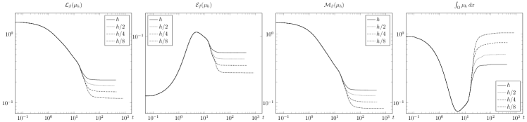
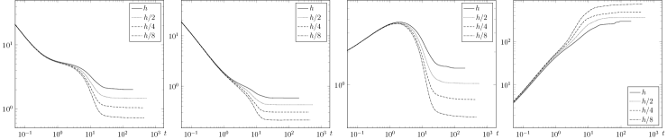
Figure 8. Time evolution of $\mathcal{L}_{\beta}(\mu_{h}(t))$, $\mathcal{E}_{f}(\mu_{h}(t))$, $\mathcal{M}_{\beta}(\mu_{h}(t))$, and $\int_{\Omega}\mu_{h}(t)\,dx$ (left to right) for TC1 (top) and TC2 (bottom), for all grid refinement levels, in the case $\beta=1.5$ $\boldsymbol{\mu}^{0}\equiv 1$.

Behavior of the Lyapunov-candidate functional

We conjecture that the converged numerical solutions actually correspond to local minima for $\mathcal{L}_{\beta}$. Thus we look at the time evolution of the Lyapunov-candidate functional $\mathcal{L}_{\beta}(\mu_{h}(t))$ and its constituents $\mathcal{E}_{f}(\mu_{h}(t))$, $\mathcal{M}_{\beta}(\mu_{h}(t))$, and $\int_{\Omega}(\mu_{h}(t))$. Figure 8 shows the time evolution of these components at the different refinement levels, using $\beta=1.5$ and $\boldsymbol{\mu}^{0}\equiv 1$ as starting data. All the plots show an initial common behavior followed by a distinct pattern as a function of $h$. Intuitively, higher resolutions allow better exploration of the state space and thus better asymptotic optimality, possibly leading to varying structures. It is interesting to note that the behavior for both TC1 and TC2 is consistent inasmuch as lower $h$ leads to lower values of $\mathcal{L}_{\beta}$. Moreover, differences of the equilibrium $\mathcal{L}_{\beta}$-value at consecutive mesh levels remain constant, corresponding to the constant ratio between subsequent $h$ parameters. These numerical simulations support the statements in Proposition 1 on the decrease in time of the $\mathcal{L}_{\beta}(\mu_{h}(t))$. Note that similar results are obtained for all powers $\beta$, initial data $\boldsymbol{\mu}^{0}$, and for both forcing terms considered. The presence of local minima is typically accompanied by sensitivity to initial conditions. Indeed, unlike the case $\beta\leq 1$, we observe this dependence, which in our cases clearly influences the asymptotic value $\mathcal{L}_{\beta}(\mu_{h}^{*})$.

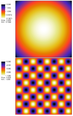
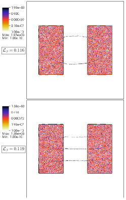
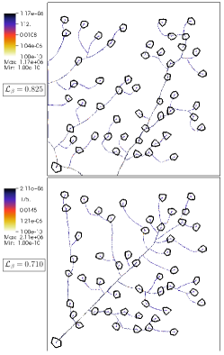
Figure 9. Spatial distribution of initial data $\boldsymbol{\mu}^{0}_{i}$ for $i=2,3$ (left panel), and the corresponding asymptotic state $\mu_{h}^{*}$ for TC1 (center) and TC2 (right) for the finest mesh and $\beta=1.5$. The value of the Lyapunov-candidate functional $\mathcal{L}_{\beta}$ is displayed on the box under the color scale. The color scale is limited at the minimum threshold of $10^{-10}$.

Table 1. Values of the Lyapunov-candidate functional $\mathcal{L}_{\beta}(\mu_{h}^{*})$ for $\beta=1.5$ in test cases TC1 and TC2 for different initial conditions.

IC	TC1	TC2	IC	TC1	TC2	IC	TC1	TC2
$\boldsymbol{\mu}^{0}_{1}$	0.116	0.722	$\boldsymbol{\mu}^{0}_{2}$	0.116	0.825	$\boldsymbol{\mu}^{0}_{3}$	0.119	0.710

Sensitivity to initial conditions

In this paragraph the above-mentioned dependence upon the initial condition $\boldsymbol{\mu}^{0}$ is explored by running both TC1 and TC2 starting from different spatial patterns. While the case $\boldsymbol{\mu}^{0}_{1}=1$ is shown in the previous sections, in Figure 9 we report the $\mu_{h}^{*}$ behavior obtained on the finest grid and for $\beta=1.5$ starting from $\boldsymbol{\mu}^{0}_{2}$ and $\boldsymbol{\mu}^{0}_{3}$, whose spatial distributions is shown in the left column. In the case of $\boldsymbol{\mu}^{0}_{2}$, where initial data attain their minimum value of $0.01$ at the center of the square, the supports of the equilibrium configurations of both TC1 and TC2 seem to avoid, altogether regions of lower initial density. On the other hand, an oscillatory starting configuration leads to added aggregating and distributive areas in the supports of $f^{+}$ and $f^{-}$. For TC1 this leads to the formation an additional central channel connecting $f^{+}$ and $f^{-}$. In TC2, the resulting tree seems closer to the one obtained with uniform ICs ($\boldsymbol{\mu}^{0}_{1}$) rather than to the case of central penalization ($\boldsymbol{\mu}^{0}_{2}$). This sensitivity to initial conditions suggests that the separate network patterns noted in Figure 6 are a result of both better resolution and different time-step size sequences, hinting at the presence of local minima from which the dynamics is not able to evade. Indeed, the value of $\mathcal{L}_{\beta}(\mu_{h}^{*})$ (summarized in table 1) in the case of three central channels (TC3) is larger than in the other two cases. On the other hand, for TC2, similar $\mathcal{L}_{\beta}$ values are achieved for $\boldsymbol{\mu}^{0}_{1}$ and $\boldsymbol{\mu}^{0}_{3}$, with $\boldsymbol{\mu}^{0}_{2}$ being higher. Note that the fact that $\boldsymbol{\mu}^{0}_{3}$ results in a smaller value of $\mathcal{L}_{\beta}$ with respect to the $\boldsymbol{\mu}^{0}_{1}$ solution can be intuitively justified by observing from the spatial patterns shown in Figures 6 and 9 that the checkerboard initial condition promotes connections between nodes that are more straight with respect to case of uniform IC. These results seem to indicate a rather flat optimization horizon with a number of similar minima towards which our dynamics leans as a function of the initial conditions.

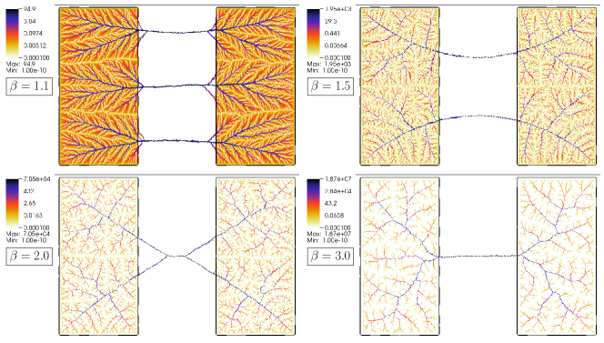
Figure 10. Behavior of the spatial distribution of $\mu^{*}_{\beta}$ for TC1 for different values of $\beta$. The color scale starts from $10^{-4}$, but the white regions indicate where $\mu^{*}_{\beta}$ attains the minimum threshold value of $10^{-10}$.

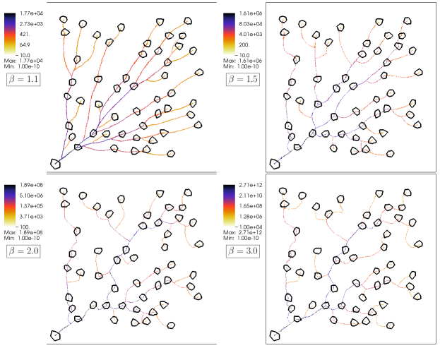
Figure 11. Behavior of the spatial distribution of $\mu^{*}_{\beta}$ for TC2 for different values of $\beta$. The color scales start from different initial values, but the white regions indicate where $\mu^{*}_{\beta}$ attains the minimum threshold value of $10^{-10}$.

Sensitivity to $\beta$

This paragraph explores the sensitivity of the proposed model to the power $\beta\in(1.1,1.5,2,3)$. Figures 10 and 11 report $\mu_{h}^{*}$ obtained for the different values of $\beta$ on the finest grid using uniform initial data $\boldsymbol{\mu}^{0}_{1}$ for TC1 and TC2, respectively. Looking at TC1, for increasing values of $\beta$ the proposed dynamics tends to create networks that seem to increasingly promote concentration. Channels characterized by larger transport density seem to be sparser and the source and sink areas are connected by fewer singular structures. In fact, the number of central channels created at the equilibrium varies from three for $\beta=1.1$ to one for $\beta=3$, with the final configuration showing no branching points in the central channel. In the TC2 case, a number of topological changes in the emerging networks are clearly noticed in the sequence. Moreover, inaccuracies emerge in the form of curve-shaped connections between branching points approximating the expected straight lines. These inaccuracies grow as $\beta$ increases and are clearly visible already for $\beta=2.0$. We argue that they are caused by the combined effects of grid alignment and the dependence upon the initial data, leading to a configuration possibly related to a local minimum of the Lyapunov-candidate functional.

For both test cases we note branching angles that increase with $\beta$, as observed in the BT theory of Xia [23] for decreasing values of $q$. Analogously, for TC2 the branching points move progressively away from the source nodes at increasing $\beta$. These results suggest that $\beta$ must increase as $q$ decreases.

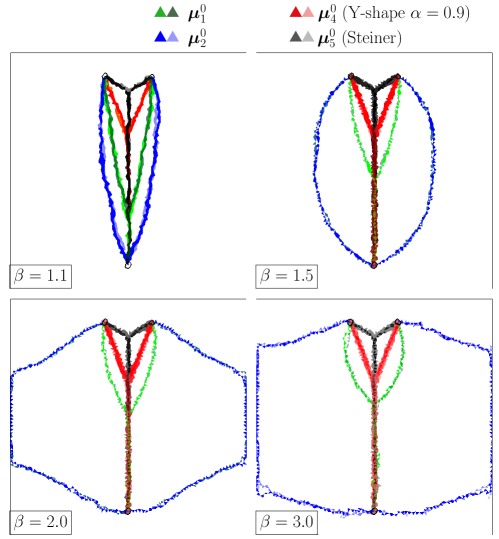
Figure 12. Spatial distribution of $\mu_{h}^{*}$ for TC3 starting form different initial data, as identify by different colors. The green and blue curves are obtained using $\boldsymbol{\mu}^{0}_{1}$ and $\boldsymbol{\mu}^{0}_{2}$, respectively. The red and the black curves report the solutions obtained by using an initial distribution concentrated along the Y-shaped known solution of the standard branched transport problem for $q=0.9,0$. The different panels show the equilibrium configurations of $\mu_{h}$ for $\beta=1.1,1.5,2.0,3.0$. Additionally, each color is represented with two different intensities to show the solutions obtained with two different meshes of the same size but different node distribution. The color scale is limited at the minimum threshold of $10^{-10}$.

Test Case 3

TC3 is designed to address two fundamental questions arising from the results of TC1 and TC2. First, we would like to explore the influence on $\mu_{h}^{*}$ of the grid geometry and of the initial data $\mu_{0}$. Then we would like to acquire some intuition on a possible relationship $\beta(q)$, in addition to the above observation that it must be a decreasing function. In this test case the optimal vector field $v^{*}$ solution of Eq. 4 is supported on a Y-shaped graph that branches at a point with coordinates $(0.5,c(q))$ with $c(q)$ a function that grows from $0.1$ for $q=1.0$ to $0.8422$ for $q=0.0$ [26]. Note that the latter value of $q$ corresponds to Steiner problem, for which the path branches at constant angles equal to $2/3\pi$. Figure 12 shows a number of simulation results for different values of $\beta$, different initial conditions, and different meshes. Each curve in a panel displays the large-time solution obtained with initial condition specified by the color codes in the top legend. In particular, the green and blue curves correspond to $\boldsymbol{\mu}^{0}_{1}$ and $\boldsymbol{\mu}^{0}_{2}$, respectively. The initial conditions identified with $\boldsymbol{\mu}^{0}_{4}$ and $\boldsymbol{\mu}^{0}_{5}$, (red and gray, respectively) are the projection on $\mathcal{T}_{h}$ of the BT Y-shaped transport path for $q=0.9$ and $q=0$. For each initial guess, we show two numerical solutions obtained from simulations run with two different triangulations of the same size but varying nodal distribution, identified with the same color but different intensity. The results reported in Figure 12 suggests that the choice of the initial data $\mu_{0}$ has a much stronger influence on the steady state configuration $\mu_{h}^{*}$, than the triangulation $\mathcal{T}_{h}$ used in the discretization of  Eq. 2. In fact, we note that, independently on the initial data $\mu_{0}$ or the power $\beta$, the supports of $\mu_{h}^{*}$ reported in Figure 12 with darker and lighter colors clearly concentrate on the same limit structure, which is only marginally influenced by the topological constraint imposed a-priori by the graph associated with the triangulation.

On the other hand, we clearly notice that the supports of $\mu_{h}^{*}$ tend to concentrate on regions where $\mu_{0}$ is larger, a behavior already observed in TC1 and TC2. For $\mu_{0}=\boldsymbol{\mu}^{0}_{4},\boldsymbol{\mu}^{0}_{5}$, the dynamics is not able to drive $\mu_{h}$ away from the strongly pre-imposed paths. For $\mu_{0}=\boldsymbol{\mu}^{0}_{2}$, $\mu_{h}^{*}$ distributes on two separate branches concentrating on regions with initially higher conductivities. Such behavior is more pronounced as $\beta$ grows. For the case $\mu_{0}=\boldsymbol{\mu}^{0}_{1}$, where the initial data is uniformly distributed and there is no a-priori bias, the support of $\mu_{h}^{*}$ forms a Y-like shape, with a bifurcation point at $(0,c(\beta))$ with $c(\beta)$ that is gradually increasing with $\beta$. However, we note how the point $(0,c(\beta))$ does not quite reach the bifurcation point $(0,c(q))$ of the reference solution for $q=0.9$ even for the largest value $\beta=3.0$.

Unfortunately, the only conclusion that can be deduced from this and the other test cases not reported here is the already mentioned decreasing behavior of $\beta(q)$. The strong dependence of our dynamics on the initial data does not allow a more accurate characterization of this relation.

4. Conclusions and discussion

We have presented and discussed an extension of the DMK model where the transient equation for $\mu$ is modulated by a power law of the transport flux with exponent $\beta>0$. The original DMK model introduced in [12] is a subset of the version discussed in this paper when $\beta=1$.

We conjecture that, for $0<\beta<1$, the long-time limit of the extended DMK model is equivalent to a $p$-Poisson Equation for $p=(2-\beta)/(1-\beta)$, and, consequently, it is equivalent to the CTP. Theoretical and numerical evidence support our claims and show that the extended DMK represents a new dynamic formulation of the $p$-Poisson equation and can be proposed as a relaxation for the efficient numerical solution of $p$-Laplacian.

In the case $\beta>1$, we claim a link between the steady state solution $(\mu^{*},u^{*})$ of our extended DMK model and solutions of BTPs. In this case, the complex solutions emerging from our dynamics remind of singular distributions typical of branched transport problems. However, when comparing both theoretically and numerically our BTP with the more classical BTP studied, e.g., in Xia [23], Santambrogio [20], Oudet and Santambrogio [17], Xia [25, 26], Pegon et al. [18] differences arise. In primis we need to acknowledge that our formulation, being based on the FEM approach, is based on densities that can be approximated with the Lebesgue measure. Next, we are not able to formulate an exact relationship between the equilibrium configurations $(\mu^{*},u^{*})$ and the more classical solutions of BTP. On the other hand, several numerical examples strengthen our confidence that our approach leads to interesting solutions that are promising in the quest for numerical solutions of BTPs. Indeed, our approach seems to be efficient and robust enough to produce trusty results at least for distributed sources.

References

- Banavar et al. [1999] J. R. Banavar, A. Maritan, and A. Rinaldo. Size and form in efficient transportation networks. Nature, 399(6732):130–132, May 1999.
- Banavar et al. [2014] J. R. Banavar, T. J. Cooke, A. Rinaldo, and A. Maritan. Form, function, and evolution of living organisms. Proc. Nat. Acad. Sci., 111(9):3332–3337, Mar. 2014.
- Barrett and Liu [1993] J. W. Barrett and W. Liu. Finite element approximation of the p-Laplacian. Math. Comp., 61(204):523–537, 1993.
- Benamou and Carlier [2015] J.-D. Benamou and G. Carlier. Augmented Lagrangian methods for transport optimization, mean field games and degenerate elliptic equations. J. Opt. Theory. Appl., 167(1):1–26, 2015.
- Bergamaschi et al. [2017] L. Bergamaschi, E. Facca, A. Martínez Calomardo, and M. Putti. Spectral preconditioners for the efficient numerical solution of a continuous branched transport model. J. Comput. Appl. Math., Submitted, 2017.
- Bouchitté et al. [1997] G. Bouchitté, G. Buttazzo, and P. Seppecher. Shape optimization solutions via Monge-Kantorovich equation. C. R. Math. Acad. Sci. Paris, 324(10):1185–1191, 1997.
- Brasco and Petrache [2014] L. Brasco and M. Petrache. A continuous model of transportation revisited. Journal of Mathematical Sciences (United States), 196(2):119–137, 2014. ISSN 15738795. doi: 10.1007/s10958-013-1644-7.
- Burger et al. [2018] M. Burger, J. Haskovec, P. Markowich, and H. Ranetbauer. A mesoscopic model of biological transportation networks. ArXiv e-prints, May 2018.
- Buttazzo et al. [2009] G. Buttazzo, C. Jimenez, and E. Oudet. An optimization problem for mass transportation with congested dynamics. SIAM J. Control Optim, 48(3):1961–1976, 2009. ISSN 03630129.
- Ekeland and Témam [1999] I. Ekeland and R. Témam. Convex Analysis and Variational Problems. Classics in Applied Mathematics. Society for Industrial and Applied Mathematics, 1999. ISBN 9780898714500.
- Evans and Gangbo [1999] L. C. Evans and W. Gangbo. Differential equations methods for the Monge–Kantorovich mass transfer problem, volume 653. American Mathematical Soc., 1999.
- Facca et al. [2018a] E. Facca, F. Cardin, and M. Putti. Towards a stationary Monge–Kantorovich dynamics: The Physarum Polycephalum experience. SIAM J. Appl. Math., 78(2):651–676, 2018a.
- Facca et al. [2018b] E. Facca, S. Daneri, F. Cardin, and M. Putti. Numerical solution of Monge-Kantorovich equations via a dynamic formulation. SIAM J. Sci. Comput., Submitted., 2018b.
- Glowinski and Marroco [1975] R. Glowinski and A. Marroco. Sur l’approximation, par éléments finis d’ordre un, et la résolution, par pénalisation-dualité d’une classe de problèmes de dirichlet non linéaires. Revue française d’automatique, informatique, recherche opérationnelle. Analyse numérique, 9(R2):41–76, 1975.
- Haskovec et al. [2015] J. Haskovec, P. Markowich, and B. Perthame. Mathematical analysis of a pde system for biological network formation. Communications in Partial Differential Equations, 40(5):918–956, 2015. doi: 10.1080/03605302.2014.968792. URL https://doi.org/10.1080/03605302.2014.968792.
- Hu and Cai [2013] D. Hu and D. Cai. Adaptation and optimization of biological transport networks. Phys. Rev. Lett., 111:138701, Sep 2013. doi: 10.1103/PhysRevLett.111.138701. URL https://link.aps.org/doi/10.1103/PhysRevLett.111.138701.
- Oudet and Santambrogio [2011] E. Oudet and F. Santambrogio. A Modica-Mortola approximation for branched transport and applications. Arch. Rational Mech. Anal., 201(1):115–142, 2011.
- Pegon et al. [2018] P. Pegon, F. Santambrogio, and Q. Xia. A fractal shape optimization problem in branched transport. J. Math. Pure Appl., 2018. in print.
- Rinaldo et al. [2014] A. Rinaldo, R. Rigon, J. R. Banavar, A. Maritan, and I. Rodriguez-Iturbe. Evolution and selection of river networks: statics, dynamics, and complexity. Proc. Nat. Acad. Sci., 111(7):2417–2424, Feb. 2014.
- Santambrogio [2010] F. Santambrogio. A Modica–Mortola approximation for branched transport. C. R. Math. Acad. Sci. Paris, 348(15):941–945, 2010.
- Santambrogio [2015] F. Santambrogio. Optimal transport for applied mathematicians. Birkäuser, NY, 2015.
- Tero et al. [2007] A. Tero, R. Kobayashi, and T. Nakagaki. A mathematical model for adaptive transport network in path finding by true slime mold. J. Theor. Biol., 244(4):553–564, Feb. 2007.
- Xia [2003] Q. Xia. Optimal paths related to transport problems. Comm. Cont. Math., 5(02):251–279, 2003.
- Xia [2010] Q. Xia. Notice of retraction numerical simulation of optimal transport paths. In Computer Modeling and Simulation, 2010. ICCMS’10. Second International Conference on, volume 1, pages 521–525. IEEE, 2010.
- Xia [2014] Q. Xia. On landscape functions associated with transport paths. Discr. Cont. Dyn. Sys., 34(4):1683–1700, 2014.
- Xia [2015] Q. Xia. Motivations, ideas and applications of ramified optimal transportation. ESAIM-Math. Model. Num., 49(6):1791–1832, 2015.