Large Datasets, Bias and Model Oriented Optimal Design of Experiments

Abstract

We review recent literature that proposes to adapt ideas from classical model based optimal design of experiments to problems of data selection of large datasets. Special attention is given to bias reduction and to protection against confounders. Some new results are presented. Theoretical and computational comparisons are made.

1 Introduction

For the analysis of big datasets statistical methods have been developed which use the full available dataset. For example new methodologies developed in the context of big data and focussed on a “divide-and-recombine” approach are summarised in wang2015statistical . Other two major methods address the scalability of big data through Bayesian inference based on a Consensus Monte Carlo algorithm scott2016bayes and sparsity assumptions tibshirani2015statistical .

In contrast other authors argue on the advantages of inference statements based on a well-chosen subset of the big dataset. Below we review some algorithms and papers for the model based selection of subsamples from a large dataset. While usually data can be collected in scientific studies via active or passive observation, big data is often collected in passive way. Rarely their collection is the result of a designed process. This generates sources of bias which either we do not know at all or are too costly to control. Nevertheless they will affect the overall distribution of the observed variables dunson2018 ; pescecladag .

Many authors in specialIssueStatProbLetters argues that analysis of big data set is effected by issues of bias and confounding, selection bias and other sampling problems (e.g. sharpes2018 for electronic health records). Often the causal effect of interest can only be measured on the average and great care has to be taken about the background population. The analysis of the full dataset might be prohibitive because of computational and time constraints. Indeed in some cases the analysis of the full dataset might also be not advisable Harford2014 . To recall just one example, Meng2018 reports that the simple sample proportion of a self-reported big dataset of size $2,300,000$ unit has the same mean squared error as the sample proportion from a suitable simple random sample of size $400$ and a Law of Large Population has been defined in order to qualify this.

Recently some researchers argued on the usefulness of utilising methods and ideas from Design of Experiment (DoE) for the analysis of big datasets, more specifically from model-based optimal experimental design. They argue that special models are useful, or even needed, to guard against hidden sources of bias and that a well-chosen subset of the big dataset can deliver equivalent answers compared to the full dataset at considerably less effort. For example one can resort to using randomization or latent variable methods. In Section 2 we review some of those papers (see also flassig2018model ) distinguishing models without bias, models with bias and no confounders, and models with confounders and no bias. We make some steps towards the generalisation to include both bias and confounders in Section 3. Theoretical and computational comparisons made using the software R lead us to conclude that so far these approaches are more suitable for tall dataset than for genuine large datasets and indicate that much work is needed to have efficient algorithms for subsample selection from large datasets in the presence of bias and confounders. To fix terminology we recall that a dataset is tall if the number of observations is much larger than the number of predictors, and large when it has many observations and predictors.

2 Model oriented selection of sub-dataset

The most general form of the considered model is that of a linear model for a response variable $\boldsymbol{Y}$

$$\boldsymbol{Y}(\boldsymbol{x},\boldsymbol{z})=\boldsymbol{f}^{\prime}(\boldsymbol{x})\boldsymbol{\theta}+\boldsymbol{h}^{\prime}(\boldsymbol{x})\boldsymbol{\psi}+\boldsymbol{g}^{\prime}(\boldsymbol{z})\boldsymbol{\phi}+\epsilon$$ (1)

with $\boldsymbol{\theta}\in\mathbb{R}^{p}$, $\boldsymbol{\psi}\in\mathbb{R}^{m}$ and $\boldsymbol{\phi}\in\mathbb{R}^{q}$ and with $\boldsymbol{x}\in\mathcal{X}$, $\boldsymbol{z}\in\mathcal{Z}$. The observed values are on the $\boldsymbol{x}$, while the $\boldsymbol{z}$ are unknown. Both the $\mathcal{X}$ and $\mathcal{Z}$ spaces are assumed to be finite and ^′ indicates transpose. The usual assumptions are taken on the random errors: $\epsilon_{i}$ are iid and $\operatorname{Var}(\epsilon_{i})=\sigma^{2}$. There are three terms in the model: the first corresponds to a classical linear model, the second to a bias term related to the variables $\boldsymbol{x}$ and the last term models a bias that may result from confounders, sources of bias which either we do not know at all or are too costly to control. We assume it to be linear for simplicity of comparison.

Special cases of the Model in Equation (1) have been addressed in order to adapt ideas from classical model based optimal DoE: montepiedra and wiens consider $\boldsymbol{f}^{\prime}(\boldsymbol{x})\boldsymbol{\theta}+\boldsymbol{h}^{\prime}(\boldsymbol{x})\boldsymbol{\psi}$, while pescecladag considers $\boldsymbol{f}^{\prime}(\boldsymbol{x})\boldsymbol{\theta}+\boldsymbol{g}^{\prime}(\boldsymbol{z})\boldsymbol{\phi}$. All search for a design which minimises the mean square error of the least square estimate (LSE) of the $\boldsymbol{\theta}$ parameters, guarding against the two different sources of bias. Recently, authors of drovandi and stufken proposed methods of data selection from large datasets in a DoE context, as a response to the more and more frequent need to analyse Big Data. However they do not guard against different sources of bias. We review these first.

2.1 Model without bias

In this section we consider the model $\operatorname{E}\left[Y(\boldsymbol{x})\right]=\boldsymbol{f}(\boldsymbol{x})^{\prime}\,\boldsymbol{\theta}$ and the two algorithms presented in drovandi and stufken . An optimal experimental design perspective is suggested in drovandi , where a retrospective sample set is drawn in accordance with a sampling plan or experimental design. Analysis and inference are then based on this designed sample. This approach is targeted towards applications of regression models with large number of observations and relative small number of predictors, otherwise the problem of finding the best subset of data becomes computationally hard or infeasible due to the curse of dimensionality.

The pseudocode of the algorithm is presented in Algorithm 1. The input to the algorithm is the support vector of the mean of a linear model, $\boldsymbol{f}$, a utility function $U$ based on $\boldsymbol{f}$, a distance function in $\mathcal{X}$ and a tall dataset called Data with typical row $(\boldsymbol{x},\boldsymbol{y}(\boldsymbol{x}))$ with $\boldsymbol{x}\in{\bf Data}\subset\mathcal{X}$. In drovandi various $U$ functions are considered and the Euclidean distance. The output of the algorithm is a subset of $n_{d}$ data points from Data which maximises some expected utility $U$, where $n_{d}$ is much smaller than the number of points in $\mathcal{X}$.

The key idea behind the algorithm is to “cluster” $\mathcal{X}$, or to “discretise” it, into a grid. Then $\boldsymbol{\theta}$ is estimated using an initial random sample from $\mathcal{X}$. Next the grid point $\boldsymbol{d^{\ast}}$ maximising $U$ is found and one or more $\boldsymbol{x}$ points in Data which are closest to $\boldsymbol{d^{\ast}}$ with respect to specified distance are added to the random sample. This is repeated until a subset of size $n_{d}$ is obtained.

Algorithm 1 Sample selection from Data based on $\operatorname{E}\left[Y(\boldsymbol{x})\right]{=}\boldsymbol{f}(\boldsymbol{x})^{\prime}\,\boldsymbol{\theta}$ according to drovandi

1:Fix a grid on $\mathcal{X}$

2:Sample randomly a subset of size $n_{t}<n_{d}$ from the Data and obtain the estimate of ${\boldsymbol{\theta}}$ or form a prior density function $p(\boldsymbol{\theta})$. Set the current sample size $n_{c}=n_{t}$

3:while $n_{c}\leq n_{d}$ or when a certain criteria is not met do

4:     Find the grid point $\boldsymbol{d^{\ast}}$ such that $\boldsymbol{d^{\ast}}{=}\underset{\boldsymbol{d}}{\operatorname{argmax}}\,\mathbb{E}[U(\boldsymbol{d},\boldsymbol{\theta},{\boldsymbol{y}}(\boldsymbol{d}))]$

5:     Find $\boldsymbol{x}$ in Data and not already sampled, which minimizes the distance $||\boldsymbol{x}-\boldsymbol{d}^{\ast}||$

6:     Add $(\boldsymbol{x},\boldsymbol{y}(\boldsymbol{x}))$ into the data subset, remove the observation $(\boldsymbol{x},\boldsymbol{y}(\boldsymbol{x}))$ from Data and set $n_{c}\leftarrow n_{c}+1$ (steps 5 and 6 may be performed multiple times to sub-sample a batch of data of size $m$, and setting $n_{c}\leftarrow n_{c}+m$)

7:     Re-estimate ${\boldsymbol{\theta}}$ or update the prior distribution $p(\boldsymbol{\theta})$

8:     go to while

The major features of Algorithm 1 is that it returns a subset of Data via an optimal, sequential and response adaptive procedure. The computations of the distances in point 5. and the optimisation problem in point 4. can be parallelised, thus speeding it up considerably. Parallelization is particularly useful when the stopping criterion, the utility function and/or the distance function are costly to evaluate or when the sampling grid is large. Its major drawback is that it requires full trust in the model. Also although it can be adapted for variable selection, the algorithm is efficient only for tall datasets, indeed point 5. and the computation of $U$ may suffer from the curse of dimensionality. Finally we note that the obtained optimal design can be used as train set of, e.g., a random forest, giving interesting results (see Example 1).

The second algorithm we present appears in stufken and is called IBOSS (Information-Based Optimal Subdata Selection). It is a deterministic algorithm to select the most informative data points for the model $\operatorname{E}\left[Y(\boldsymbol{x})\right]=\boldsymbol{f}(\boldsymbol{x})^{\prime}\,\boldsymbol{\theta}$. A pseudocode is given in Algorithm 2. The rational behind IBOSS is that $D$-optimal designs tend to be on the boundary of the available space. The selected points are shown to be optimal in the following sense.

Let Data have $N$ points. Data can coincide with $\mathcal{X}$. A subset of Data of size $n_{d}$ is sought which maximises a univariate optimality criterion function $\Psi$ of the information matrix

$$\boldsymbol{M}(\boldsymbol{\delta})=\frac{1}{\sigma^{2}}\sum_{i=1}^{N}\delta_{i}\boldsymbol{x}_{i}\boldsymbol{x}_{i}^{\prime}\,\,\text{ subject to }\sum_{i=1}^{N}\delta_{i}=n_{d}$$

where $\delta_{i}=1$ if point $i\in$ Data is selected and $\delta_{i}=0$ otherwise. The function $\Psi$ could be the determinant of $\boldsymbol{M}$, expressing thus $D$-optimality. In stufken the following inequality is proven for the $D$-optimality criterion

$$\operatorname{det}(\boldsymbol{M}(\boldsymbol{\delta}))\leq 4\left(\frac{n_{d}}{4\sigma^{2}}\right)^{p+1}\prod_{j=1}^{p}(x_{(N)j}-x_{(1)j})^{2}$$

where $x_{(N)j}-x_{(1)j}$ is the observed range of the $j$th variable and $\sigma^{2}$ is the model variance. This gives a function easy to optimize and larger than the desired utility function. Thus the optimal design is obtained by selecting iteratively $r{=}n_{d}/(2p)$ data points on the boundary of the observed range of each predictor. If $\frac{n_{d}}{2p}$ is not integer, one can clearly take floor or ceiling or choose a suitable $n_{d}$. Note that the full sample $\mathcal{X}$ does not need to be specified nor it is used. But the representativeness of Data for $Y$ in $\mathcal{X}$ has to be trusted.

We found the algorithm to work better for tall datasets and tested it for up to one million points in four variables (much larger datasets are considered in stufken ). It proved to be cost effective and can be parallelised. It requires full trust in the model and the output depends on the initial ordering of the variables in Step 3, as shown in the small two dimensional example in Figure 1 where the designs obtained starting with the variable $x_{1}$ (in red) or $x_{2}$ (in green) can be very different. For special cases a symmetry argument or a group action could be employed to establish the equivalence of the obtained design.

Algorithm 2 Pseudocode for IBOSS stufken

1:Assume $r=n_{d}/(2p)$ integer

2:Initialise selected sample $\boldsymbol{\delta}^{\ast}=\emptyset$

3:for $j=1,\ldots,p$ do

4:     for $1\leq i\leq N$ do

5:         if $j>2$ then

6:              $\textbf{Data}\longleftarrow\textbf{Data}\setminus\boldsymbol{\delta}^{\ast}$          

7:         Add the $r$ points with the smallest $x_{ij}$ value to $\boldsymbol{\delta}^{\ast}$

8:         Add the $r$ points with the largest $x_{ij}$ values to $\boldsymbol{\delta}^{\ast}$      

9:     end

10:end

11:Obtain an estimate of $\boldsymbol{\theta}$ with the selected $n_{d}$ data points

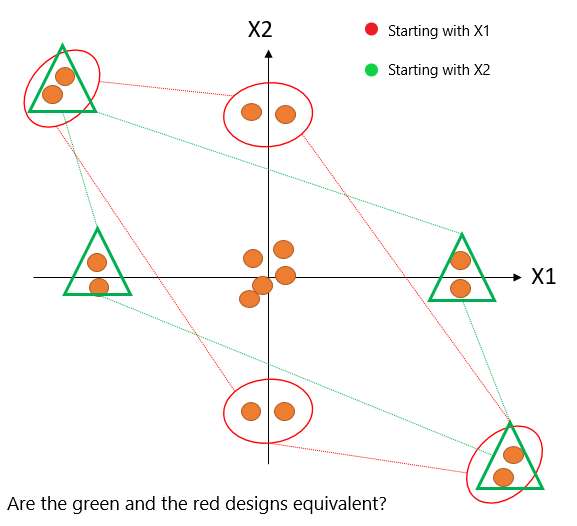
Figure 1: Effect of the initial ordering of the factors on the IBOSS output

2.2 Models with no confounders terms

The model of the form $\boldsymbol{Y}(\boldsymbol{x})=\boldsymbol{f}(\boldsymbol{x})^{\prime}\boldsymbol{\theta}+\boldsymbol{h}(\boldsymbol{x})^{\prime}\boldsymbol{\psi}+\boldsymbol{\epsilon}$ is considered in wiens . The sample space $\mathcal{X}$ is assumed to be a discrete finite set $\mathcal{X}=\left\{\boldsymbol{x_{1}},\ldots,\boldsymbol{x_{N}}\right\}$ and $\mathcal{X}$ can be thought of as the grid discretising the sample space in drovandi .

Several methods are presented in wiens for the construction of designs that are minimax robust for linear or nonlinear models whose mean structures cannot be guaranteed to have been specified with complete accuracy. (Actually the author considers a more general bias term than the one above, specifically the model $\operatorname{E}\left[Y(\boldsymbol{x})\right]=\boldsymbol{f}(\boldsymbol{x})^{\prime}\,\boldsymbol{\theta}+\psi(\boldsymbol{x})$ under the constraint $\sum_{\boldsymbol{x}\in\mathcal{X}}\boldsymbol{f}(\boldsymbol{x})\psi(\boldsymbol{x})=0$ which ensures identifiability.) The classical notions of $I$- and $D$-optimality are extended by taking into account the bias of the predictions and a minimax $I$- and $D$-robust design theory is developed. Imposing a neighbourhood structure on the regression response function, the proposed methods maximise the mean squared error over this neighbourhood, and then seek $I$- and $D$- robust designs that minimize this maximum loss.

Formally, let $\hat{\boldsymbol{\theta}}$ be the LSE of $\boldsymbol{\theta}$ based on a design $\boldsymbol{\xi}$. The two loss functions

$$\mathcal{I}(\psi,\boldsymbol{\xi}){=}\sum_{\boldsymbol{x}\in\chi}\mathbb{E}\left[\left(\boldsymbol{f}^{\prime}(\boldsymbol{x})\hat{\boldsymbol{\theta}}-\mathbb{E}[Y(\boldsymbol{x})]\right)^{2}\right]\quad\text{and}\quad\mathcal{D}(\psi,\boldsymbol{\xi}){=}\left(\operatorname{det}\mathbb{E}\left[(\hat{\boldsymbol{\theta}}-\boldsymbol{\theta})(\hat{\boldsymbol{\theta}}-\boldsymbol{\theta})^{\prime}\right]\right)^{1/p}$$

can be factorised as

$$\max_{\psi}\mathcal{I}(\psi,\boldsymbol{\xi}){=}\frac{\sigma^{2}+\tau^{2}}{n}\times\mathcal{I}_{\nu}(\boldsymbol{\xi})\quad\text{and}\quad\max_{\psi}\mathcal{D}(\psi,\boldsymbol{\xi}){=}\frac{\sigma^{2}}{n}\left(\frac{\sigma^{2}+\tau^{2}}{\sigma^{2}\operatorname{det}[\boldsymbol{F}^{\prime}\boldsymbol{F}]}\right)^{1/p}\times\mathcal{D}_{\nu}(\boldsymbol{\xi})$$

where $\mathcal{I}_{\nu}$ and $\mathcal{D}_{\nu}$ depend only on the sought design and on known quantities. Here $\boldsymbol{F}=\left[\boldsymbol{f}(\boldsymbol{x})\right]_{\boldsymbol{x}\in\mathcal{X}}$ is the full model matrix. The objective is to find $\underset{\boldsymbol{\xi}}{\operatorname{min}}\,\,\underset{\psi}{\operatorname{max}}\,\,\mathcal{D}(\psi,\boldsymbol{\xi})$ or $\underset{\boldsymbol{\xi}}{\operatorname{min}}\,\,\underset{\psi}{\operatorname{max}}\,\,\mathcal{I}(\psi,\boldsymbol{\xi})$.

In more details $\sigma^{2}$ is the model variance, $\tau$ a control parameter and $n$ the number of points in the design $\boldsymbol{\xi}$ with non zero probability mass. The design measure is indicated with $\boldsymbol{\xi}=\left\{\begin{array}[]{l}\boldsymbol{x}\\ \boldsymbol{\xi}_{\boldsymbol{x}}\end{array}\right\}_{\boldsymbol{x}\in\mathcal{X}}$ and can be collected in a diagonal matrix $\boldsymbol{D}(\boldsymbol{\xi})=\operatorname{diag}\left(\boldsymbol{\xi}_{\boldsymbol{x}}:\boldsymbol{x}\in\mathcal{X}\right)$. The key factors in $\mathcal{I}(\psi,\boldsymbol{\xi})$ and $\mathcal{D}(\psi,\boldsymbol{\xi})$ are

$$\mathcal{I}_{\nu}(\boldsymbol{\xi}) =(1-\nu)\operatorname{tr}\boldsymbol{R}^{-1}(\boldsymbol{\xi})+\nu\lambda_{max}\left(\boldsymbol{U}(\boldsymbol{\xi})\right)$$

$$\mathcal{D}_{\nu}(\boldsymbol{\xi}) =\left(\frac{1-\nu+\nu\lambda_{max}\left(\boldsymbol{R}^{1/2}(\boldsymbol{\xi})[\boldsymbol{U}(\boldsymbol{\xi})-\boldsymbol{I}_{p}]R^{1/2}(\boldsymbol{\xi})\right)}{\det[\boldsymbol{R}(\boldsymbol{\xi})]}\right)^{1/p}$$

where $\nu=\tau^{2}/(\sigma^{2}+\tau^{2})$, $\boldsymbol{I}_{p}$ the $p\times p$ identity matrix, $\lambda_{max}$ is the maximum eigenvalue. The control parameter $\nu$ is in $[0,1]$. For $\nu=0$, then $\mathcal{D}_{0}(\boldsymbol{\xi})$ gives the classical D-optimality and $\mathcal{I}_{0}(\boldsymbol{\xi})$ the classical I-optimality. For given $\nu\in(0,1]$ a design $\boldsymbol{\xi}$ on $\chi$ is defined to be I-robust if it minimizes $\mathcal{I}_{\nu}(\boldsymbol{\xi})$ in the class of all designs on $\chi$, and D-robust if it minimizes $\mathcal{D}_{\nu}(\boldsymbol{\xi})$. If $\nu=1$ then the uniform design is D-/I- robust.

The algorithm proposed in wiens is based on the QR-decomposition of $\boldsymbol{F}$, where $\boldsymbol{Q}$ is the $Q$-matrix in such decomposition, and finally

$$\boldsymbol{R}(\boldsymbol{\xi})=\boldsymbol{Q}^{\prime}\boldsymbol{D}(\boldsymbol{\xi})\boldsymbol{Q}\quad\text{ and }\quad\boldsymbol{U}(\boldsymbol{\xi})=\boldsymbol{R}^{-1}(\boldsymbol{\xi})\boldsymbol{Q}^{\prime}\boldsymbol{D}^{2}(\boldsymbol{\xi})\boldsymbol{Q}\boldsymbol{R}^{-1}(\boldsymbol{\xi})$$

Algorithm 3 Wiens approach for D-robustness and $\nu\neq 0,1$

1:Let the sample space be $\mathcal{X}=\{\boldsymbol{x_{i}}\}_{i=1,\ldots,N}$ and $\boldsymbol{e}_{i}$ the $i$-th column of the $I_{N}$ identity matrix, QR-decomposition of $\boldsymbol{F}$

2:Sample randomly a subset of size $n_{t}<n_{d}$ from the sample space ($n_{t}=1$ is ok). Set the current sample size $n=n_{t}$ and $\boldsymbol{\xi}=\left\{\begin{matrix}\boldsymbol{x}\\ \boldsymbol{\xi_{n,\boldsymbol{x}}}\end{matrix}\right\}_{\boldsymbol{x}\in\mathcal{X}}$

3:while $n\leq n_{d}$ or when a certain criteria is not met do

4:     compute • $\lambda$ maximum eigenvalue of $\boldsymbol{R}^{1/2}(\boldsymbol{\xi})[\boldsymbol{U}(\boldsymbol{\xi})-\boldsymbol{I}_{p}]R^{1/2}(\boldsymbol{\xi})$ • and $\boldsymbol{z}$ the corresponding eigenvector • the vectors $\boldsymbol{v}(\boldsymbol{\xi}){=}\boldsymbol{R}^{1/2}(\boldsymbol{\xi})\boldsymbol{z}(\boldsymbol{\xi})$ and $\boldsymbol{w}(\boldsymbol{\xi}){=}\boldsymbol{R}^{-1/2}(\boldsymbol{\xi})\boldsymbol{z}(\boldsymbol{\xi})$ • the matrices $\displaystyle\boldsymbol{J}(\boldsymbol{\xi})$ $\displaystyle=\lambda\left(\boldsymbol{R}^{-1}(\boldsymbol{\xi})+\boldsymbol{w}(\boldsymbol{\xi})\boldsymbol{w}^{\prime}(\boldsymbol{\xi})\right)+\left(\boldsymbol{w}(\boldsymbol{\xi})\boldsymbol{v}^{\prime}(\boldsymbol{\xi})+\boldsymbol{v}(\boldsymbol{\xi})\boldsymbol{w}^{\prime}(\boldsymbol{\xi})\right)$ $\displaystyle\boldsymbol{K}(\boldsymbol{\xi})$ $\displaystyle=2\boldsymbol{w}(\boldsymbol{\xi})\boldsymbol{w}^{\prime}(\boldsymbol{\xi})$ • and $$T(\boldsymbol{\xi})=(1-\nu)\boldsymbol{Q}\boldsymbol{R}^{-1}(\boldsymbol{\xi})\boldsymbol{Q}^{\prime}+\nu[\boldsymbol{Q}\boldsymbol{J}(\boldsymbol{\xi})\boldsymbol{Q}^{\prime}-\boldsymbol{D}(\boldsymbol{\xi})\boldsymbol{Q}\boldsymbol{K}(\boldsymbol{\xi})\boldsymbol{Q}^{\prime}],$$ • the largest diagonal element of $T(\boldsymbol{\xi})$ and assume it is in entry $(i,i)$

5:     Update the weights of $\boldsymbol{\xi_{n,\boldsymbol{x}}}$ to $\boldsymbol{\xi_{n+1,\boldsymbol{x}}}=\left(\frac{n}{n+1}\right)\left(\boldsymbol{\xi}_{n}+\frac{1}{n}\boldsymbol{e}_{i}\right)$

6:     go to while.

The pseudocode is given in Algorithm 3. Its main features are that bias is accounted for and the optimal design is known prior observing. The method is supported by strong theoretical background. As given the algorithm is purely sequential, but it can be tweaked to become adaptive. Unfortunately it requires the QR-decomposition of a high dimensional matrix and requires to keep in memory large matrices. Current available implementation is not very performing but a smart implementation may overcome some of these issues and make the algorithm efficient for significatively large sample sizes.

Next we recall some precursory work on optimal subdata collection for linear regression based on the information matrix montepiedra which, we believe, is useful in the presence of big data. For $\xi_{\boldsymbol{x}}$ as above, the information matrix can be written as

$$M=\int_{\mathcal{X}}\left(\begin{matrix}\boldsymbol{f}\\ \boldsymbol{h}\end{matrix}\right)\left(\boldsymbol{f}^{\prime},\boldsymbol{h}^{\prime}\right)\,d\,\xi_{\boldsymbol{x}}=\left[\begin{array}[]{cc}M_{11}&M_{12}\\ M_{21}&M_{22}\end{array}\right]$$

where $M_{11}$ depends only on $\boldsymbol{f}$ and $M_{22}$ depends only on $\boldsymbol{g}$. The mean square error of the LSE of $\theta$ is $\mathbb{E}\{(\hat{\boldsymbol{\theta}}-\boldsymbol{\theta})(\hat{\boldsymbol{\theta}}-\boldsymbol{\theta})^{\prime}\}{=}\sigma^{2}N^{-1}R$ where

$$R=M_{11}^{-1}{+}\left(\frac{N}{\sigma}\right)^{2}M_{11}^{-1}M_{12}\boldsymbol{\psi}\boldsymbol{\psi}^{\prime}M_{21}M_{11}^{-1}$$

and the loss function for $D$-optimality becomes

$$\operatorname{det}(R)=\operatorname{det}(M_{11}^{-1})\,\left(1+\left(\frac{N}{\sigma}\right)^{2}\boldsymbol{\psi}^{\prime}M_{21}M_{11}^{-1}M_{12}\boldsymbol{\psi}\right)$$

A $D$-optimal design for bias reduction satisfies the following optimisation problems

$$\xi^{\ast}=\underset{\xi}{\operatorname{argmax}}\operatorname{det}(M_{11})\text{ such that }\left(\frac{N}{\sigma}\right)^{2}\boldsymbol{\psi}^{\prime}M_{21}M_{11}^{-1}M_{12}\boldsymbol{\psi}\leq B$$

for a given $B$. (The authors in montepiedra also study variance reduction but here we focus on bias reduction as far more relevant in the analysis of big data.) Thus the objective becomes to determine $\xi^{\ast}=\operatorname{argmax}_{\xi}\operatorname{det}(M_{11})$ such that $\left(\frac{N}{\sigma}\right)^{2}\boldsymbol{\psi}^{\prime}M_{21}M_{11}^{-1}M_{12}\boldsymbol{\psi}\leq B$. A design $\xi^{\ast}$ is optimal if and only if there exists $\lambda^{\ast}\geq 0$ such that

$$d_{1}(\boldsymbol{x},\xi^{\ast})+\lambda^{\ast}d_{2}(\boldsymbol{x},\xi^{\ast})\leq p-\lambda^{\ast}B$$

for all $\boldsymbol{x}\in\mathcal{X}$, where

$$d_{1}(\boldsymbol{x},\xi) =\boldsymbol{f}(\boldsymbol{x})^{\prime}M_{11}^{-1}\boldsymbol{f}(\boldsymbol{x})\,\,\text{ and }\,\,d_{2}(\boldsymbol{x},\xi)=\phi^{2}(\boldsymbol{x},\xi)-2\phi(\boldsymbol{x},\xi)r(\boldsymbol{x})$$

with

$$r(\boldsymbol{x}) =\frac{N}{\sigma}\boldsymbol{\psi}^{\prime}\boldsymbol{h}(\boldsymbol{x})\,\,\text{ and }\,\,\phi(\boldsymbol{x},\xi)=\int_{\mathcal{X}}\boldsymbol{f}(\boldsymbol{x})^{\prime}M_{11}^{-1}\boldsymbol{f}(\boldsymbol{x}^{\prime})\xi(d\boldsymbol{x}^{\prime})$$

This gives a strong theoretical background and makes a good link with the next sections but does not provide specific algorithms nor applies to big data directly.

2.3 Models with no bias terms

Models of the form $\boldsymbol{Y}(\boldsymbol{x,z})=\boldsymbol{f}(\boldsymbol{x})^{\prime}\boldsymbol{\theta}+\boldsymbol{g}(\boldsymbol{z})^{\prime}\boldsymbol{\phi}+\boldsymbol{\epsilon}$ have been considered in pescecladag . Let $\xi_{\boldsymbol{x,z}}$ be a design measure on $\mathcal{X}\times\mathcal{Z}$. The information matrix is

$$M={\int}_{\mathcal{X}\times\mathcal{Z}}\left(\begin{matrix}\boldsymbol{f}\\ \boldsymbol{g}\end{matrix}\right)\left(\boldsymbol{f}^{\prime},\boldsymbol{g}^{\prime}\right)\,d\,\xi_{\boldsymbol{x,z}}$$

The mean square error of the LSE of $\theta$ is $\sigma^{2}N^{-1}R$ where

$$R=M_{11}^{-1}{+}\left(\frac{N}{\sigma}\right)^{2}M_{11}^{-1}M_{12}\boldsymbol{\phi}\boldsymbol{\phi}^{\prime}M_{21}M_{11}^{-1}$$

and the loss function for $D$-optimality depends on both $\boldsymbol{x}$ and $\boldsymbol{z}$ and it is

$$\operatorname{det}(R)=\operatorname{det}(M_{11}^{-1})\,\left(1+\left(\frac{N}{\sigma}\right)^{2}\boldsymbol{\phi}^{\prime}M_{21}M_{11}^{-1}M_{12}\boldsymbol{\phi}\right)$$

We assume $\boldsymbol{g}(\boldsymbol{z})^{\prime}\boldsymbol{\phi}$ unknown, belonging to some function class. For each $\boldsymbol{x}\in\textbf{Data}$ there is an unobserved $\boldsymbol{z_{x}}\in\mathcal{Z}$. Let $\boldsymbol{G}=[\boldsymbol{g}(\boldsymbol{z_{x}})]_{\boldsymbol{x}\in\textbf{Data}}$ and $P_{Z}$ be a randomization distribution for the $\boldsymbol{z_{x}}$’s. In the game theoretical approach in pescecladag , a $D$-optimal design measure is one maximising

$$\underset{P_{Z}}{\min}~{}\mathbb{E}_{P_{Z}}\left\{\max_{\begin{subarray}{c}\text{ \small{function}}\\ \text{\small{class}}\end{subarray}}\,\boldsymbol{G}^{\prime}\boldsymbol{\phi}\boldsymbol{F}M_{11}^{-2}\boldsymbol{F}^{\prime}\boldsymbol{\phi}^{\prime}\boldsymbol{G}\right\}$$

3 General formulation: model with bias and confounders

In this section we consider the more general form for the response variable $\boldsymbol{Y}$ in Model (1), define the variance function to be $d((\boldsymbol{x},\boldsymbol{z}),\boldsymbol{\xi})=\boldsymbol{f}^{\prime}(\boldsymbol{x})M(\boldsymbol{\xi})^{-1}\boldsymbol{f}(\boldsymbol{x})$ and assume that $M(\boldsymbol{\xi})$ is a closed and bounded subset of the semi-definite positive matrices. Then a version of the General Equivalence Theorem for Model (1) holds.

Theorem 3.1

For a design measure $\boldsymbol{\xi}^{\ast}$ the following statements are equivalent

1. $\boldsymbol{\xi}^{\ast}$ maximizes $\operatorname{det}(M(\boldsymbol{\xi}))$

2. $\boldsymbol{\xi}^{\ast}$ achieves $\min_{\boldsymbol{\xi}}\max_{(x,z)\in\mathcal{X}\times\mathcal{Z}}d((\boldsymbol{x},\boldsymbol{z}),\boldsymbol{\xi})$

3. $\max_{(x,z)\in\mathcal{X}\times\mathcal{Z}}d((\boldsymbol{x},\boldsymbol{z}),\boldsymbol{\xi}^{\ast})=p+m+q-2$.

Proof

There are two further equivalent conditions which allows a circular proof. One is a local D-optimality condition

$$\emph{(iv)}\frac{\partial}{\partial(\boldsymbol{x},\boldsymbol{z})}\log\operatorname{det}\left(M\left(\left(1-\alpha\right)\boldsymbol{\xi}^{\ast}+\alpha\boldsymbol{\xi}^{\prime}\right)\right)\mid_{\alpha=0}\,\leq\,\boldsymbol{0}$$

where $\boldsymbol{\xi}^{\ast}$ and $\boldsymbol{\xi}^{\prime}$ are design measures. The fifth equivalent condition is

$$\emph{(v)}\,\,d((\boldsymbol{x},\boldsymbol{z}),\boldsymbol{\xi})\leq p+m+q-2\,\,\,\text{ for all }(\boldsymbol{x},\boldsymbol{z})\in\mathcal{X}\times\mathcal{Z}$$

That Item (i) implies (iv) is straigthforward. To show that Item (iv) implies (v) we use the matrix identity $\frac{\partial}{\partial\alpha}\log\operatorname{det}(A)=\operatorname{tr}\left(A^{-1}\frac{\partial A}{\partial\alpha}\right).$. Thus

$$\frac{\partial}{\partial(\boldsymbol{x},\boldsymbol{z})}\log \operatorname{det}\left(M\left(\left(1-\alpha\right)\boldsymbol{\xi}^{\ast}+\alpha\boldsymbol{\xi}^{\prime}\right)\right)\mid_{\alpha=0}$$

$$=\operatorname{tr}\left(M^{-1}\left(\left(1-\alpha\right)\boldsymbol{\xi}^{\ast}+\alpha\boldsymbol{\xi}^{\prime}\right)\cdot\frac{\partial}{\partial\alpha}M\left(\left(1-\alpha\right)\boldsymbol{\xi}^{\ast}+\alpha\boldsymbol{\xi}^{\prime}\right)\right)\mid_{\alpha=0}$$

$$=\operatorname{tr}\left(M^{-1}\left(\left(1-\alpha\right)\boldsymbol{\xi}^{\ast}+\alpha\boldsymbol{\xi}^{\prime}\right)\cdot\frac{\partial}{\partial\alpha}\left((1-\alpha)M(\boldsymbol{\xi}^{\ast})+\alpha M(\boldsymbol{\xi}^{\prime})\right)\right)\mid_{\alpha=0}$$

$$=\operatorname{tr}\left(M^{-1}\left(\left(1-\alpha\right)\boldsymbol{\xi}^{\ast}+\alpha\boldsymbol{\xi}^{\prime}\right)\cdot\left(-M(\boldsymbol{\xi}^{\ast})+M(\boldsymbol{\xi}^{\prime})\right)\right)\mid_{\alpha=0}$$

$$=\operatorname{tr}\left(M^{-1}(\boldsymbol{\xi}^{\ast})\cdot(-M(\boldsymbol{\xi}^{\ast})+M(\boldsymbol{\xi}^{\prime}))\right)\ =\operatorname{tr}\left(-I_{p+m+q-2}+M^{-1}(\boldsymbol{\xi}^{\ast})M(\boldsymbol{\xi}^{\prime})\right)$$

$$=-(p+m+q-2)+\operatorname{tr}\left(\int_{\mathcal{X}\times\mathcal{Z}}d((\boldsymbol{x},\boldsymbol{z}),\boldsymbol{\xi}^{\ast})\,\boldsymbol{\xi}^{\prime}(dx,dz)\right)$$

so that the statement in (iv) is equivalent to $\int_{\mathcal{X}\times\mathcal{Z}}d((\boldsymbol{x},\boldsymbol{z}),\boldsymbol{\xi}^{\ast})\,\boldsymbol{\xi}^{\prime}(dx,dz)\leq p+m+q-2$ for all $\boldsymbol{\xi}^{\prime}$. This holds in particular when $\boldsymbol{\xi}^{\prime}$ places mass one at a specific point $(\boldsymbol{x},\boldsymbol{z})$. But this is $d((\boldsymbol{x},\boldsymbol{z}),\boldsymbol{\xi}^{\ast})\leq p+m+q-2$ for all $(\boldsymbol{x},\boldsymbol{z})$, so (v) is verified.

To prove that (iii) is equivalent to (iv), we can show that

$$\max_{(x,z)\in\mathcal{X}\times\mathcal{Z}}d((\boldsymbol{x},\boldsymbol{z}),\boldsymbol{\xi}^{\ast})\geq p+m+q-2\text{ for all }(\boldsymbol{x},\boldsymbol{z})$$

But this follows from the fact that a maximum is always greater than or equal to an average, so

$$\max_{(x,z)\in\mathcal{X}\times\mathcal{Z}}d((\boldsymbol{x},\boldsymbol{z}),\boldsymbol{\xi}^{\ast}) \geq\int_{\mathcal{X}\times\mathcal{Z}}d((\boldsymbol{x},\boldsymbol{z}),\boldsymbol{\xi}^{\ast})\,\boldsymbol{\xi}^{\ast}(dx,dz)$$

$$=\operatorname{tr}\left(M^{-1}(\boldsymbol{\xi}^{\ast})M(\boldsymbol{\xi}^{\ast})\right)=\operatorname{tr}(I_{p+m+q-2})=p+m+q-2$$

As we assumed that $M(\boldsymbol{\xi})$ is a closed and bounded subset of the semi-definite positive matrices, $\boldsymbol{\xi}^{\ast}$ achieves the bound

Lastly we prove that (iii) implies (i). We use the identity $\operatorname{tr}(A)\geq n\cdot\operatorname{det}(A)^{\frac{1}{n}}$ for an $n\times n$ matrix $A$. Thus for $k=p+m+q-2$ we have

$$k =\max_{(x,z)\in\mathcal{X}\times\mathcal{Z}}d((\boldsymbol{x},\boldsymbol{z}),\boldsymbol{\xi}^{\ast})\geq\int_{\mathcal{X}\times\mathcal{Z}}d((\boldsymbol{x},\boldsymbol{z}),\boldsymbol{\xi}^{\ast})\,\boldsymbol{\xi}^{\prime}(dx,dz)$$

$$=\operatorname{tr}\left(M^{-1}(\boldsymbol{\xi}^{\ast})M(\boldsymbol{\xi}^{\prime})\right)\geq k\cdot\operatorname{det}\left(M^{-1}(\boldsymbol{\xi}^{\ast})M(\boldsymbol{\xi}^{\prime})\right)^{\frac{1}{k}}$$

$$=k\cdot\left(\operatorname{det}\left(M^{-1}(\boldsymbol{\xi}^{\ast})\right)\operatorname{det}\left(M(\boldsymbol{\xi}^{\prime})\right)\right)^{\frac{1}{k}}=k\cdot\left(\frac{\operatorname{det}(M(\boldsymbol{\xi}^{\prime}))}{\operatorname{det}(M(\boldsymbol{\xi}^{\ast}))}\right)^{\frac{1}{k}}$$

From this $\operatorname{det}(M(\boldsymbol{\xi}^{\ast}))\geq\operatorname{det}(M(\boldsymbol{\xi}^{\prime}))$, which is (i); so we have (iii) holds if and only if (i) holds. ∎

3.1 Guard against bias

In analogy to Subsection 2.3, we want to protect the usual LSE of $\boldsymbol{\theta}$ in Model (1) against the two bias terms $\boldsymbol{\psi}$ and $\boldsymbol{\phi}$. The information matrix for a $\xi_{\boldsymbol{x},\boldsymbol{z}}$ design measure on $\mathcal{X}\times\mathcal{Z}$ can be written as

$$M=M(\boldsymbol{\xi})={\int}_{\mathcal{X}\times\mathcal{Z}}\left(\begin{matrix}\boldsymbol{f}\\ \boldsymbol{h}\\ \boldsymbol{g}\end{matrix}\right)\left(\boldsymbol{f}^{\prime},\boldsymbol{h}^{\prime},\boldsymbol{g}^{\prime}\right)\,d\,\xi_{\boldsymbol{x,z}}=\left[\begin{array}[]{ccc}M_{11}&M_{12}&M_{13}\\ M_{21}&M_{22}&M_{23}\\ M_{31}&M_{32}&M_{33}\end{array}\right]$$

where by symmetry $M_{12}$ is the transpose of $M_{21}$ and so on. The mean square error matrix of the LSE of $\boldsymbol{\theta}$ is $\sigma^{2}N^{-1}R$ where $N$ is the sample size, $\sigma^{2}$ the common variance of the error terms for the Model (1) and where

$$R=M_{11}^{-1}{+}\left(\frac{N}{\sigma}\right)^{2}M_{11}^{-1}\left[M_{12}~{}M_{13}\right]\left[\boldsymbol{\psi}~{}\boldsymbol{\phi}\right]^{\prime}\left[\boldsymbol{\psi}^{\prime}~{}\boldsymbol{\phi}^{\prime}\right]\left[\begin{array}[]{c}M_{21}\\ M_{31}\end{array}\right]^{\prime}M_{11}^{-1}$$

Above we gave an elementary proof of a General Equivalence Theorem in order to get a relation between optimality criteria (D-, G- and A-optimality). In this subsection we are interested in minimising loss functions of the matrix $R$. Future work will focus on making a relation between the loss functions of $M(\boldsymbol{\xi})$ and $R$, in order to use the General Equivalence Theorem also for the matrix $R$. In particular, here we concentrate on the A-optimality and derive a formula for $\operatorname{tr}(R)$

$$\operatorname{tr}(R)= \operatorname{tr}\left(M_{11}^{-1}{+}\left(\frac{N}{\sigma}\right)^{2}M_{11}^{-1}\left[M_{12}~{}M_{13}\right]\left[\boldsymbol{\psi}~{}\boldsymbol{\phi}\right]^{\prime}\left[\boldsymbol{\psi}^{\prime}~{}\boldsymbol{\phi}^{\prime}\right]\left[M_{21}~{}M_{31}\right]^{\prime}M_{11}^{-1}\right)$$

$$= \operatorname{tr}\left(M_{11}^{-1}\right)+\left(\frac{N}{\sigma}\right)^{2}\operatorname{tr}\left(M_{11}^{-1}\right.$$

$$\left.\left[M_{12}\boldsymbol{\psi}\boldsymbol{\psi}^{\prime}M_{21}+M_{13}\boldsymbol{\phi}\boldsymbol{\phi}^{\prime}M_{31}+M_{12}\boldsymbol{\psi}\boldsymbol{\phi}^{\prime}M_{31}+\left(M_{12}\boldsymbol{\psi}\boldsymbol{\phi}^{\prime}M_{31}\right)^{\prime}\right]M_{11}^{-1}\right)$$

$$= \operatorname{tr}\left(M_{11}^{-1}\right)+\left(\frac{N}{\sigma}\right)^{2}\operatorname{tr}\left(M_{11}^{-1}M_{12}\boldsymbol{\psi}\boldsymbol{\psi}^{\prime}M_{21}M_{11}^{-1}\right)+\left(\frac{N}{\sigma}\right)^{2}\operatorname{tr}\left(M_{11}^{-1}M_{13}\boldsymbol{\phi}\boldsymbol{\phi}^{\prime}M_{31}M_{11}^{-1}\right)$$

$$+2\left(\frac{N}{\sigma}\right)^{2}\operatorname{tr}\left(M_{11}^{-1}M_{12}\boldsymbol{\psi}\boldsymbol{\phi}^{\prime}M_{31}M_{11}^{-1}\right)$$

$$= \operatorname{tr}(M_{11}^{-1})+\left(\frac{N}{\sigma}\right)^{2}\operatorname{tr}(S_{2})+\left(\frac{N}{\sigma}\right)^{2}\operatorname{tr}(S_{3})+2\left(\frac{N}{\sigma}\right)^{2}\operatorname{tr}(S_{4})$$

where

$$\operatorname{tr}(S_{2}) =\operatorname{tr}\left(M_{11}^{-1}M_{12}\boldsymbol{\psi}\boldsymbol{\psi}^{\prime}M_{21}M_{11}^{-1}\right)=\operatorname{tr}\left(\boldsymbol{\psi}^{\prime}M_{21}M_{11}^{-1}M_{11}^{-1}M_{12}\boldsymbol{\psi}\right)$$

$$=\boldsymbol{\psi}^{\prime}M_{21}M_{11}^{-2}M_{12}\boldsymbol{\psi}$$

$$\operatorname{tr}(S_{3}) =\boldsymbol{\phi}^{\prime}M_{31}M_{11}^{-2}M_{13}\boldsymbol{\phi}$$

$$\operatorname{tr}(S_{4}) =\boldsymbol{\phi}^{\prime}M_{31}M_{11}^{-2}M_{12}\boldsymbol{\psi}$$

and thus

$$\operatorname{tr}(R) =\operatorname{tr}\left(M_{11}^{-1}\right)$$ (2)

$$+\left(\frac{N}{\sigma}\right)^{2}\left(\boldsymbol{\psi}^{\prime}M_{21}M_{11}^{-2}M_{12}\boldsymbol{\psi}+\boldsymbol{\phi}^{\prime}M_{31}M_{11}^{-2}M_{13}\boldsymbol{\phi}+\boldsymbol{\phi}^{\prime}M_{31}M_{11}^{-2}M_{12}\boldsymbol{\psi}\right)$$

In $\operatorname{tr}(R)$, the first and second terms depend only on $\boldsymbol{x}$ and te third term on $\boldsymbol{x}$ and on $\boldsymbol{z}$ but not on the bias $\boldsymbol{h}$. When the foruth term is equal to zero, then the minimization of the $\operatorname{tr}(R)$ can be done separately on the $\boldsymbol{x}$ variables and the $\boldsymbol{z}$ variables and generalization to non linear confounders is easier.

4 Examples and simulations

Example 1

Algorithm 1 is applied on the simulated mortgage defaults (year 2000) dataset analysed in drovandi . The dataset has $1,000,000$ data points, a binary response for the mortgage default $Y_{i}\sim\text{\emph{Binary}}(\pi_{i})$ and four covariates: credit Score ($\boldsymbol{x}_{1}$), age of the house in years ($\boldsymbol{x}_{2}$), number of years the mortgage holder has been employed at current job ($\boldsymbol{x}_{3}$) and amount of credit card debt ($\boldsymbol{x}_{4}$). The scaled values of the data points are clustered around the grid in Table 1, so we take this as the grid used in Algorithm 1. The response is skewed: $Y_{i}=1$ in 1031 units and $Y_{i}=0$ for $998,969$ units and following drovandi we assume $Y_{i}\sim\text{\emph{Binary}}(\pi_{i})$ and a logistic model $\text{\emph{logit}}(\pi_{i})=\theta_{0}+\theta_{1}x_{1i}+\theta_{2}x_{2i}+\theta_{3}x_{3i}+\theta_{4}x_{4i}$.

Covariate	Grid
creditscore	-4, -3, -2, -1, 0, 1, 2, 3, 4
houseAge	-2, -1, 0, 1, 2
yearsemploy	-2, -1, 0, 1, 2, 3, 4
ccDebt	-2, -1, 0, 1, 2, 3, 4

Table 1: Grid generated by data points.

The maximum likelihood estimates of the parameters of the logit models are obtained starting with $n_{t}=5,000$ points in step 2. and with a final sample of size $n_{d}=6,200$. The estimates are consistent with those in drovandi .

Further to drovandi in Figure 2 we investigate the effect of the choice of the initial sample on the parameter estimates: black refers to an initial sample including all units for which $Y=1$ (a dope training set in machine learning), red to a randomly selected initial sample, green to a stratified sample: we considered the distribution of ccDebt for the sub-population for which $Y=1$ and sampled one data points for each quantile, since preliminary analysis indicates that ccDebt effect most the response. All the estimates converge to the same values, but the black being quicker as expected.

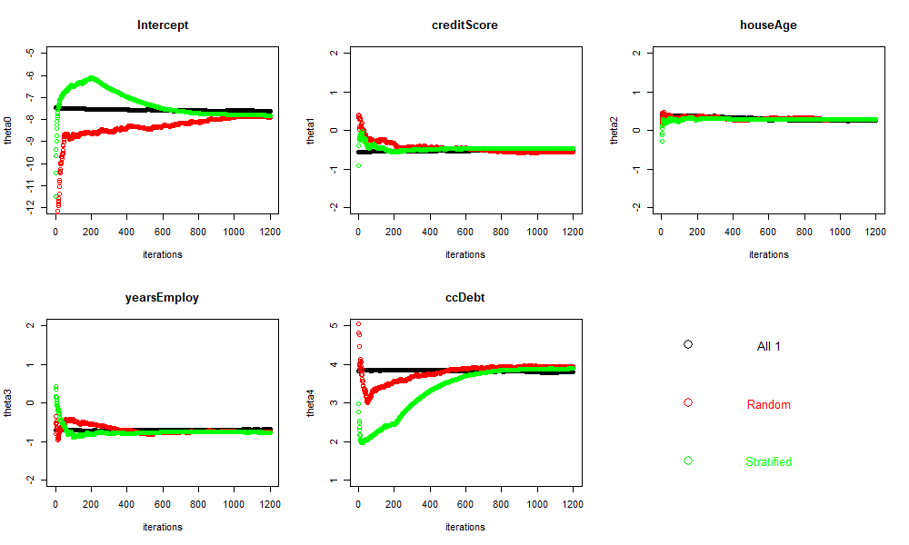
Figure 2: Effect of the initial sample on the output of Algorithm 1

The performance of Algorithm 1 in terms of the prediction of the response outcomes is tested on $10,010$ data points that are not considered above. The comparison is made with random forests (RF) and neural networks (NN) build with a random training set or with the final “best” sample obtained through Algorithm 1. The results are report in Table 2. Algorithm 1 performs better than the other approaches with a random training set, but the performance of a RF or a NN is better when starting with the best sample from Algorithm 1.

Model	Confusion matrix
Algorithm 1	$\begin{bmatrix}9765&3\\ 235&7\\ \end{bmatrix}$
RF + random train	$\begin{bmatrix}10000&10\\ 0&0\\ \end{bmatrix}$
RF + best sample	$\begin{bmatrix}9718&2\\ 282&8\\ \end{bmatrix}$
NN + random train	$\begin{bmatrix}10000&10\\ 0&0\\ \end{bmatrix}$
NN + best sample	$\begin{bmatrix}9176&0\\ 824&10\\ \end{bmatrix}$

Table 2: Confusion matrices of different methods.

Example 2

Algorithms 1 and 2 are compared on simulated data from the model $y=-x/2-5/3+0.35\,\sin(x^{2})+z/9+\epsilon$ which includes both the bias term $0.35\,\sin(x^{2})$ and the confounder term $g(z)=z/9$. Hundred and five points in $\mathbb{R}^{2}$ were generated from two independent gaussian random variables $X\sim\mathcal{N}(2,1)$ and $Z\sim\mathcal{N}(0,1)$ for the first and second component of the points, respectively. The grid used in the algorithms is given by $200$ uniformly distributed points for $x$, chosen between the minimum and the maximum generated values, and crossed with $200$ points for $z$ chosen in the same manner.

Figure 3 shows the twelve point optimal designs returned by the two algorithms (in green Algorithm 1 and in red Algorithm 2) when the $D$-optimality utility function is computed on $-x/2-5/3+z/9$. Algorithm 2 pushes the selected points more on the boundary of the $(x,z)$-plane. The plot in the left panel of Figure 4 projects the designs in Figure 3 of the response-$x$ plane, the right plot compares on the same plane the “optimal” designs returned by the two algorithms when all biases are ignored and the optimality function is thus computed on $-x/2-5/3$. As expected the outputs for the models with no confounders are very similar, begin different in just one point. Always the value of the utility function is larger for Algorithm 2.

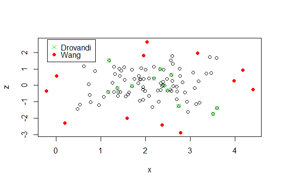
Figure 3: Outputs from Algorithms 1 in red and 2 in green for Example 2

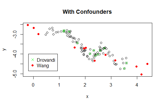
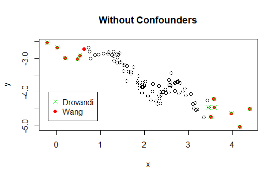
Figure 4: Different utilities for Example 2

Example 3

Next we consider $105$ integer in $-100{:}100$ and the model $x+\cos(x)+z/9+\epsilon$ with $\epsilon\sim\mathcal{N}(0,1)$. The $D$-optimal designs returned by Algorithms 1, 2 and 3 are plotted on the $x{-}z$ plane in Figure 5. In the right panel the utility function $\operatorname{det}X^{t}X$ is based only on $x$, that is does not include any information of the bias and the confounder terms. To make a comparison, isn the left panel the utility function is based on $(x,z/9)$, that is the term modelling confounders is used. The control parameter $\nu$ in Algorithm 3 is set equal to $0.5$. The grid used in the Algorithms for the $z$ is of hundred points in $-3/3$ and also hundred points were taken for the $x$ grid in $-100:100$. We tried different discretization for the grids and the results were the same.

In all our trials when comparing the designs obtained from a model, say $x$, and from a model with confounders, say $x+z/9$, Algorithms 1 and 3 give results more similar.

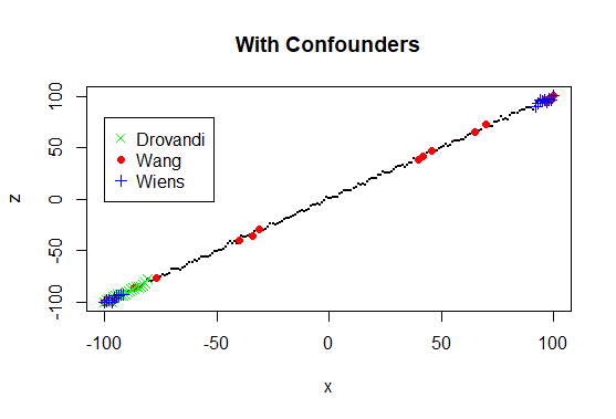
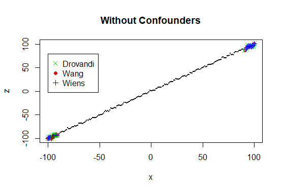
Figure 5: Different utilities for Example 3

5 Conclusions and future work

In Section 2 we reviewed literature which considers special cases of Model (1) in order to adapt ideas from classical model based optimal DoE: montepiedra and wiens consider a linear model with a bias term while pescecladag consider a linear model with confounders, searching for a design which minimises the mean square error of the LSE of the $\boldsymbol{\theta}$ parameters. Here in Section 3 we follow that but guarding against the two different sources of bias.

The algorithms in drovandi and stufken offer methods of data selection from large datasets in a DoE context, however they do not guard against different sources of bias. We are currently integrating the above ideas with those algorithms with the objective of providing efficient subsample selection methods for problems with known confounders and also with unknown confounders.

We also presented some preliminary results on a unified theory to take into account selection bias, model bias and bias due to confounders in the choice of a subsample for an efficient estimation, in the least square sense, of parameters expressing the effect of interest. Still much work is needed to turn this into an algorithm for the selection of efficient subsamples from large or big data sets. Furthermore the results in Section 3 need to be refined, possibly linking them with the algorithms in Section 2.

References

- (1) C. C. Drovandi, C. Holmes, J. M. McGree, K. Mengersen, S. Richardson and E. G. Ryan, Principles of Experimental Design for Big Data Analysis, Statistical Science, 32(3), 385–404 (2017).
- (2) D. B. Dunson, Statistics in the big data era: Failures of the machine, Statistics and Probability Letters, 136, 4–9 (2018).
- (3) J. J. Faraway and N. H. Augustin, When small data beats big data, Statistics and Probability Letters, 136, 142–145 (2018).
- (4) R. J. Flassig and R. Schenkendorf, Model-based design of experiments: Where to go?, Manuscript (2018).
- (5) T. Harford, Big data: are we making a big mistake?, Significance, December 2014, 14-19, reprint from The Financial Times (2014).
- (6) X. L. Meng, Statistical paradises and paradoxes in big data (I): law of large populations, big data paradox, and the 2016 US presidential election, The Annals of Applied Statistics, 12(2), 685–726 (2018).
- (7) G. Montepiedra and V. V. Fedorov, Minimum bias design with constraints, Journal of Statistical Planning and Inference, 63, 97–111 (1997).
- (8) E. Pesce, E. Riccomagno and H. P. Wynn, Passive and active observation: experimental design issues in big data, arXiv:1712.06916 (2017).
- (9) S. L Scott, A. W. Blocker, F. V. Bonassi, H. A. Chipman, Edward I George, and Robert E McCulloch, Bayes and big data: The consensus monte carlo algorithm, International Journal of Management Science and Engineering Management, 11(2), 78–88 (2016).
- (10) L. D.. Sharpes, The role of statistics in the era of big data: Electronic health records for healthcare research, Statistics and Probability Letters, 136, 105–110 (2018).
- (11) L. M. Sangalli (editor), The role of Statistics in the era of Big Data, Statistics and Probability Letters, 136 (Special issue).
- (12) R. Tibshirani, M. Wainwright and T. Hastie, Statistical learning with sparsity: the lasso and generalizations, Chapman and Hall/CRC (2015).
- (13) H. Wang, M. Yang and J. Stufken, Information-Based Optimal Subdata Selection for Big Data Linear Regression, Journal of the American Statistical Association (in press) (2018).
- (14) C. Wang, M. H. Chen, E. Schifano, J. Wu and J. Yan, Statistical methods and computing for big data, Statistics and its interface, 9(4), 399 (2016).
- (15) D.P. Wiens, I-robust and D-robust designs on a finite design space, Statistics and Computing 28(2), 241–258 (2018).