Fractal character of the phase ordering kinetics of a diluted ferromagnet

Abstract

We study numerically the coarsening kinetics of a two-dimensional ferromagnetic system with aleatory bond dilution. We show that interfaces between domains of opposite magnetisation are fractal on every lengthscale, but with different properties at short or long distances. Specifically, on lengthscales larger than the typical domains’ size the topology is that of critical random percolation, similarly to what observed in clean systems or models with different kinds of quenched disorder. On smaller lengthscales a dilution dependent fractal dimension emerges. The Hausdorff dimension increases with increasing dilution $d$ up to the value $4/3$ expected at the bond percolation threshold $d=1/2$. We discuss how such different geometries develop on different lengthscales during the phase-ordering process and how their simultaneous presence determines the scaling properties of observable quantities.

I Introduction

The growth of order in a system quenched across a phase transition is a paradigm of slow relaxation Bray94 ; Puri-Book ; Corberi2010 . A classical example, that we will consider in this paper, is provided by the coarsening kinetics of a ferromagnet after a quench from an equilibrium state above the critical temperature to a temperature $T_{f}$ below it. Considering a uniaxial magnet, for simplicity, the non-equilibrium evolution is characterised by an early development of domains – small scale realisation of the two symmetry related low temperature equilibrium phases – and the subsequent growth of their characteristic linear size $R(t)$.

In the clean cases, that is in the absence of any source of quenched disorder, such as impurities, external disturbances or lattice defects, the geometrical properties of ordered regions are well understood Bray94 ; Corberi2008 : domains are compact objects surrounded by interfaces which are subjected to thermal roughening. However, in the small $T_{f}$ limit and at long times, roughening effects are negligible when observed on the characteristic scale $R(t)$, and domain walls appear as regular, non fractal objects. These features are reflected by the behaviour of correlation functions, such as the structure factor Bray94 .

The geometry of the growing structure on scales much larger than the typical size of the domains, instead, is non trivial and has been investigated in two dimensions recently Arenzon07 ; Sicilia07 ; Sicilia08 ; Sicilia09 ; Blanchard12 ; Blanchard14 ; Tartaglia15 ; Blanchard17 ; Tartaglia16 ; Corberi17 ; Insalata18 ; Tartaglia18 . It was shown that, next to $R(t)$, another length $R_{p}(t)>R(t)$ is growing faster and, on scales $R(t)\ll r\ll R_{p}(t)$ the geometry is that of random percolation at criticality. This growing percolative structure invades the whole system at the size-dependent time $t_{p}(L)$ when $R_{p}(t_{p})$ becomes of the order of the linear size $L$ of the sample. The awareness of percolative features is not only important on its own, since its appearance in a strongly correlated system is unexpected and highly non-trivial, but represents also a cornerstone of one of the few existing analytical theories of phase-ordering. Indeed, since the distribution of cluster areas is exactly known in critical percolation Cardy03 , simply inferring their evolution after the quench allows one to arrive at an exact expression for the area distribution at any time Arenzon07 ; Sicilia07 . Moreover, the recognition that the systems quickly approach a critical percolation situation after a quench allowed one to understand the results on the percentage of blocked states found after quenches to zero temperature Barros09 ; Olejarz12 ; Blanchard13 .

When quenched disorder is present in the system, as it is very often the case when dealing with real materials, the understanding is poorer than in the clean cases. It is known from the theoretical study of model systems that even a tiny amount of quenched noise strongly inhibits the growth process Oh86 ; Oguz90 ; BrayHumayun ; Puri91 ; Puri93 ; Rao93 ; Rao93b ; Oguz94 ; Gyure95 ; Fisher98 ; Fisher01 ; Corberi02 ; Paul04 ; Paul05 ; Henkel06 ; Paul07 ; Aron08 ; Henkel08 ; Lippiello10 ; Park10 ; Corberi11 ; Corberi12 ; Corberi15 . This fact was confirmed in some experimental work on real materials Ikeda90 ; Schins93 ; Shenoy99 ; Likodimos00 ; Likodimos01 . The slowing down is accompanied by modifications of the scaling properties of the correlation functions with respect to those of clean systems Corberi15 ; Likodimos00 ; Likodimos01 . Despite all the above, it was shown in Corberi17 ; Insalata18 that basic properties, such as the compact geometry of the growing domains and their boundaries and the emergence of the percolative structure on scales beyond $R(t)$, remain unchanged when going from a clean two-dimensional Ising system to one with quenched disorder in the form of random fields or random bonds.

Notwithstanding the interest of the results discussed insofar, a full characterisation of the geometrical properties of coarsening in disordered ferromagnets remains a subject to be further pursued. Among the many open questions, the generality of what found in Corberi17 ; Insalata18 for the random field Ising model (RFIM) and the random bond Ising model (RBIM) needs to be investigated. In particular, the behaviour of these systems in the very asymptotic regime is unexplored because the numerical study in Corberi17 ; Insalata18 focused on the long-lasting transient regime Corberi11 ; Corberi12 before the system crosses over to the late non-equilibrium stage at a certain time $t_{cross}$.

In this paper we give a contribution to answering these and related questions by studying numerically the geometry of coarsening in a system with a different kind of quenched disorder, the bond-diluted Ising model (BDIM), namely a ferromagnetic spin system where pairwise interactions are randomly nullified with probability $d$, the dilution. We consider this model because on the one hand $t_{cross}$ is sufficiently short to allow one to enter the asymptotic stage and, on the other hand, because it was shown to possess a richer dynamical structure as compared to different disordered ferromagnetic systems Corberi13 .

Our results show profound differences between the BDIM and what was found in Corberi17 ; Insalata18 for the RFIM and the RBIM. These differences regard both the geometric features of the correlated region on scales $r<R(t)$ and the way in which the percolative structure develops for $r>R(t)$.

Studying the properties of the average squared winding angle, a quantity that probes the geometry of the interfaces, we show that, at variance with the clean case, the domain walls are fractal with a fractal dimension $D$. This Hausdorff dimension increases with $d$ up to the value $D=4/3$ expected at the bond percolation threshold $d_{c}=1/2$. To the best of our knowledge this is the first time that the fractality of interfaces has been quantified for this kind of system. Let us remark that growing domain boundaries are not fractal in the clean IM, the RFIM nor the RBIM for $t<t_{cross}$ (although they may be fractal for $t>t_{cross}$ in cases with quenched randomness).

Regarding the behaviour at large distances $r>R(t)$ our results confirm that a spanning cluster with the topology of critical random percolation also develops in the present model, as in the clean case and in the RFIM and RBIM. However, what changes here is the dynamics whereby this object develops and grows. Indeed, while in Corberi17 ; Insalata18 it was found that $R_{p}(t)$ is related to $R(t)$ in a way which is independent of the presence of disorder, on its nature (i.e. whether considering random fields or random bonds) and on its amount, here such relation depends on $d$. In particular, at $d=d_{c}$, where the bond network is itself a critical percolation cluster, we find that the property $R_{p}(t)>R(t)$ is no longer obeyed, since $R_{p}(t)$ and $R(t)$ coincide, as it could be expected.

These results, and in particular the dependencies of $D$ and $R_{p}(t)$ on the amount of disorder $d$, help us clarifying the superuniversal properties of coarsening kinetics. Superuniversality Fisher88 can be expressed as the fact that the only effect of quenched disorder is to slow down the coarsening process, namely the increase of $R(t)$, leaving other properties, such as the geometric ones, unchanged. Some numerical simulations gave support to this property in a number of systems Paul04 ; Paul05 ; Puri91 ; Puri92 ; Biswal96 ; Loureiro10 ; Gyure95 , including the RFIM and RBIM for $t<t_{cross}$ BrayHumayun ; Rao93b ; Puri93 ; Sicilia08 ; Aron08 , while other numerical studies pointed against its validity Lippiello10 ; Fisher01 ; Fisher98 ; Corberi02 ; Corberi11 ; Corberi12 . In the RFIM and the RBIM the squared winding angle discussed above does not depend on the presence of quenched disorder nor on its strength provided that distances are measured in units of $R(t)$. However, something different happens in the BDIM, since the effects of disorder cannot be simply accounted for by $R(t)$, and the scaling functions of observable quantities and the fractal dimension $D$ of the interfaces are also modified.

This paper is organised as follows: in Sec. II we define the BDIM model and some quantities that will be considered for its characterisation. In Sec. III we present and discuss the results of our simulations. We conclude the Article and discuss some open problems and future perspectives in Sec. IV.

II Model and observable quantities

We consider a system with Hamiltonian

$${\cal H}(\{S_{i}\})=-\sum_{\langle ij\rangle}J_{ij}S_{i}S_{j}+\sum_{i}H_{i}S_{i}\;,$$ (1)

where $S_{i}=\pm 1$ are Ising spin variables located at the vertices of a two-dimensional $L\times L$ square lattice that we label $i$, with $i=1,\dots,N=L^{2}$. $\langle ij\rangle$ denotes nearest neighbour sites $i$ and $j$ on the lattice. In the following we will study the bond-diluted Ising model (BDIM) where $H_{i}\equiv 0$ and the $J_{ij}$’s are uncorrelated random variables with probability $P(J_{ij})=(1-d)\,\delta_{J_{ij},J}+d\,\delta_{J_{ij},0}$, where $\delta$ is the Kronecker function, $J>0$, and $d$ is the dilution. The same Hamiltonian (1) also describes two different disordered model, the RFIM and the RBIM. Specifically, for the RFIM one has $J_{ij}\equiv J$ and $H_{i}=\pm h$ is uncorrelated in space and sampled from a symmetric bimodal distribution, whereas for the RBIM, the fields vanish $H_{i}\equiv 0$ and the ferromagnetic coupling constants are $J_{ij}=J+\delta_{ij}$, where $\delta_{ij}$ are independent random numbers extracted from a flat distribution in $[-\delta,+\delta]$, with $\delta<J$. The geometrical properties of these two models have been studied in a previous paper Corberi17 and, in the present analysis, we will often compare their behaviour to the one of the BDIM, where richer results are found.

Before studying the dynamics of the BDIM, let us review some of its equilibrium properties. Given the structure of the coupling constants, it is clear that for $d>d_{c}=1-p_{c}$, where $p_{c}$ is the bond percolation threshold ($p_{c}=1/2$ in the two-dimensional case considered here) the bond network is disconnected (in the thermodynamic limit). Hence the spin system is fragmented into separated parts and a globally ordered (magnetised) state cannot exist at any temperature, not even at $T=0$. For this reason we will restrict our attention to $d\leq d_{c}$ in the following. In this range of dilution the system undergoes a phase transition at a critical temperature $T_{c}(d)$ which decreases from $T_{c}(0)$ – the transition temperature of the usual model without dilution – to $T_{c}(d_{c})=0$ Selke98 ; Heuer92 ; Kim94 ; Stinchcombe83 . The coarsening dynamics of a ferromagnetic Ising model with dilution was studied in Burioni06 ; Burioni07 ; Burioni13 ; Corberi15 ; Park10 ; Paul07 ; Iwai93 .

A dynamic update is introduced by reversing spins with the Glauber transition rates

$$w(S_{i}\to-S_{i})=\frac{1}{2}\left[1-S_{i}\tanh\left(\frac{H^{W}_{i}}{T}\right)\right]$$ (2)

where $H^{W}_{i}$ is the local Weiss field

$$H^{W}_{i}=\sum_{j\in nn(i)}J_{ij}S_{j}\;,$$ (3)

and the sum runs over the nearest neighbours $nn(i)$ of $i$. Here and in the following we measure temperature in units of the Boltzmann constant.

We will consider an instantaneous quench in which the system is prepared at time $t=0$ in an infinite temperature equilibrium state, namely an uncorrelated one with zero magnetisation, and it is subsequently evolved by attempting spin flips according to the transition rates (2) evaluated at the final temperature $T=T_{f}$ of the quench. Periodic boundary conditions will be adopted.

Let us now define the various observables that we will consider in our study. The average size of the growing domains $R(t,d)$ will be computed as Bray94 ; Puri-Book ; Corberi2010

$$R(t,d)=L^{2}[E(t,d)-E_{eq}(d)]^{-1}\;,$$ (4)

where $E(t,d)=\langle H(t)\rangle$ is the non-equilibrium average (namely taken over different initial condition and thermal histories) of the energy at time $t$, and $E_{eq}(d)$ is the energy of the equilibrium state at $T_{f}$. Equation (4) is a standard method to determine the typical size of the domains in clean systems Bray94 and is well suited to be applied also to diluted systems, as discussed in Corberi13 ; Corberi15 .

The wrapping probability $\pi(t,d)$ is the probability that at time $t$ a connected wrapping cluster of equally aligned spins is present in the system. The wrapping cluster can cross the system in different ways. It can span the system from one side to the other horizontally or vertically. The probabilities of these events will be denoted as $\pi_{1,0}(t,d)$ and $\pi_{0,1}(t,d)$, respectively. On the square lattice one has $\pi_{0,1}(t,d)=\pi_{1,0}(t,d)$. A cluster can also span the sample in both horizontal and vertical directions, with probability $\pi_{0,0}(t,d)$. Finally, clusters can percolate along one of the two diagonal directions with equal probabilities $\pi_{1,-1}(t,d)$ and $\pi_{1,1}(t,d)$. With periodic boundary conditions the torus can be wrapped more than once but this occurs with extremely small probability and we will not consider these spanning configurations.

The fractal properties of the domain boundaries can be studied by considering the (average) squared winding angle $\langle\theta^{2}(r,t,d)\rangle$ defined as follows: at a given time, for any two points $i,j$ on the external perimeter of a cluster we compute the angle $\theta_{ij}$ (measured counterclockwise) between the tangent to the perimeter in $i$ and the one in $j$. Upon repeating the procedure for all the couples of perimeter points at distance $r$, taking the square and averaging over the non-equilibrium ensemble, $\langle\theta^{2}(r,t,d)\rangle$ is obtained. For numerical convenience we have considered only the largest cluster in the system.

Another quantity we will analyse is the pair connectedness function $C(r,t,d)$. In percolation theory Stauffer ; Saberi ; Christensen this quantity is defined as the probability that two points at distance $r$ belong to the same cluster. In spin systems we use the same definition where, in this case, two spins belong to the same cluster if they are aligned and are connected by a path of aligned spins. In order to compute this quantity at a given time we first identify all the domains of positive and negative spins. Then we evaluate $C(r,t)$ as

$$C(r,t,d)=\frac{1}{4L^{2}}\sum_{i}\sum_{i_{r}}\langle\delta_{S_{i},S_{i_{r}}}\rangle\;,$$ (5)

where $\delta_{S_{i},S_{j}}=1$ if the two spins belong to the same cluster and $\delta_{S_{i},S_{j}}=0$ otherwise, and $i_{r}$ is a site at distance $r$ from $i$.

III Numerical results

In this Section we present and discuss the outcome of our numerical simulations. These have been performed on systems with different sizes, from $91\times 91$ up to $512\times 512$, with periodic boundary conditions, and an average over $10^{4}-10^{5}$ realisations has been taken. The data presented in the following are usually obtained for the largest size ($512\times 512$), while smaller sizes are used to control finite size effects, see for instance Figs. 2 and 3 and the related discussion. We have performed quenches with $J=2$ to $T_{f}=0.75$ and $T_{f}=1$ and we found similar results in the two cases. Both these temperatures are below $T_{c}$ in the whole range of dilutions considered in our simulations. In the following, we will discuss data for $T_{f}=0.75$ unless otherwise stated.

In Fig. 1 we show the characteristic length $R(t,d)$ after the quench of systems with various dilutions. The behaviour of this quantity has been thoroughly discussed in Corberi13 ; Corberi15 and in Corberi15d for two and three dimensional systems, respectively, with both site or bond dilution. The main feature we want to stress here is the strong dependence of the growth law on the amount of disorder, a feature that is usually observed in ferromagnetic systems with any kind of quenched disorder. In particular, the usual law $R(t,0)\sim t^{1/2}$ is observed for the clean case only. The growth slows down upon increasing $d$ up to values of order $d=0.2-0.3$ and then it gets progressively faster as $d$ is further raised. This non-monotonic behaviour is interpreted in Corberi13 ; Corberi15 ; Corberi15d as due to the relatively fast growth at $d=d_{c}$ induced by the percolative structure of the bond network. Notice, however, that the kinetics is slower than in the clean case for any $d>0$.

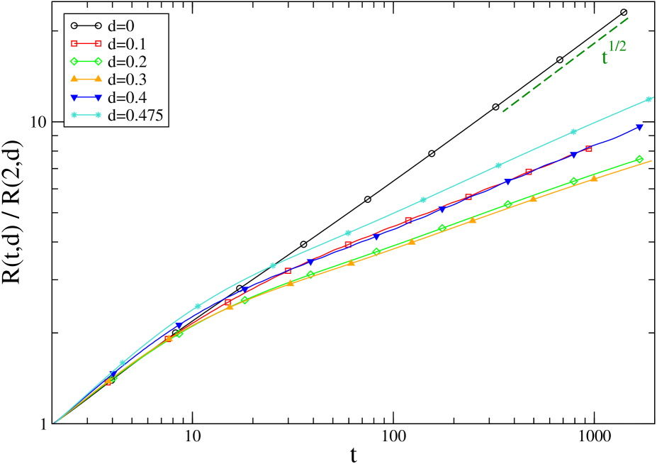
Figure 1: $R(t,d)/R(2,d)$ against time $t$ after the quench, for different choices of $d$, see the key. Dividing by $R(2,d)$ allows to better compare curves with different $d$. The dashed green line is the behaviour $t^{1/2}$ expected for the pure system with $d=0$.

Let us now discuss the behaviour of the wrapping probabilities. These quantities are exactly known for two-dimensional critical percolation under periodic boundary conditions. They are Pinson

$$\pi_{0,1}+\pi_{1,0} \simeq 0.3388\;,$$

$$\pi_{0,0} \simeq 0.61908\;,$$ (6)

$$\pi_{1,-1}+\pi_{1,1} \simeq 0.04196\;.$$

The behaviour of the wrapping probabilities during the phase-ordering process in the case without dilution is plotted in Fig. 2. In this figure, and in the following ones, we use $R(t,d)$ as a natural reparametrization of time. The wrapping probabilities start from zero immediately after the quench, because the initial state is a random mixture of an equal amount of up and down spins and there cannot be any spanning cluster in such a configuration given that the site percolation threshold ($\simeq 0.59...$) is larger than the fraction 1/2 of both kinds of spins. At long times (large $R(t,d)$) the crossing probabilities saturate to values which are very precisely consistent with the ones at critical percolation given in Eq. (6), as pointed out in Barros09 ; Olejarz12 . This fact is a first confirmation that the spanning object is a percolation cluster. These asymptotic values are attained around a certain value of $R$ that can be interpreted as $R(t_{p},d)$, where $t_{p}$ is the time when the growing percolative structure hits the system boundaries, namely $R_{p}(t_{p},d)=L$.

Comparing curves relative to systems with different size one observes that $R(t_{p},d)$ increases with $L$. This is because, as already discussed, the cluster which spans the system at $t_{p}$ does not appear altogether at that particular time but its size $R_{p}$ gradually grows until it crosses the entire system. One finds that a collapse of the wrapping probabilities for different system sizes is achieved by plotting the $\pi$’s against $R(t,d)/L^{a(d)}$, and the best collapse is obtained for $a(0)=0.178$ in this case, as shown in the inset of Fig. 2.

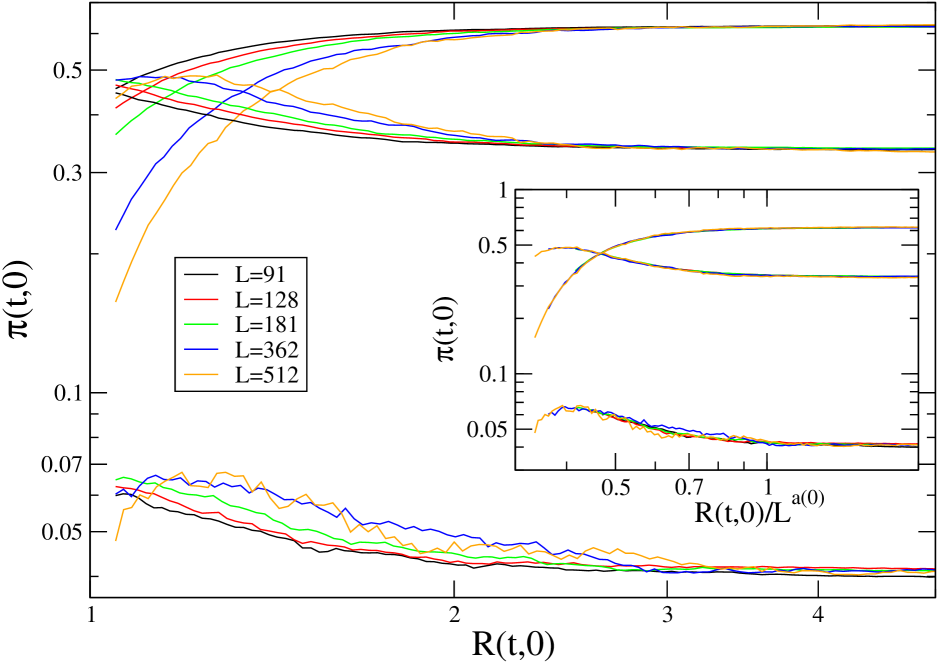
Figure 2: The wrapping probabilities $\pi(t,0)$ are plotted against $R(t,0)$ with double logarithmic scales, for $d=0$, the clean model. The curves reaching the largest saturation value correspond to the probability $\pi_{0,0}(t,0)$ (different curves are for different system sizes, see the colour code in the key). The curves reaching the lowest asymptotic value represent the probability $\pi_{1,-1}(t,0)+\pi_{1,1}(t,0)$. Finally, the remaining curves that approach an intermediate value close to 0.338 corresponds to $\pi_{0,1}(t,0)+\pi_{1,0}(t,0)$. In the inset the same quantities are plotted against $R(t,0)/L^{a(0)}$, with $a(0)=0.178$.

Before moving on to the study of the wrapping probabilities in the presence of dilution it is useful to summarise what is known for other kinds of quenched disorder, namely in the case of the RFIM and the RBIM. It was shown in Corberi17 that the presence of disorder does not change the qualitative nor the quantitative behaviour of the $\pi$’s. Indeed, by fixing the system size $L$ and plotting the crossing probabilities against $R(t)$, it was found that the curves corresponding to the clean case, the RFIM and the RBIM, fall one on top of the other, despite the fact that, as in the dilute case, the addition of frozen randomness greatly slows down the kinetics. The superposition is observed for any strength of the quenched disorder, namely for different values of $h$ and $\delta$. This property, sometimes referred to as superuniversality Fisher88 , implies that the sole effect of disorder is to change the form of $R(t)$, leaving other properties unmodified.

On the other hand, by varying the system size $L$, one can again obtain data collapse for the wrapping probabilities by plotting them against $R(t)/L^{a}$, where $a$ is an exponent which turns out to be independent both on the kind and strength of disorder.

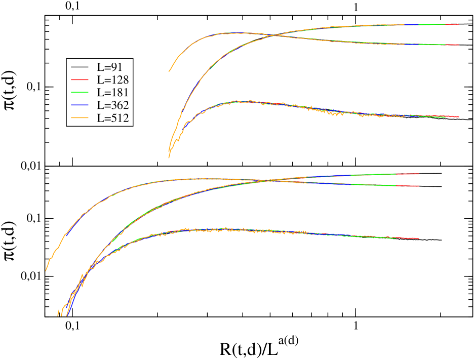
Figure 3: The wrapping probabilities $\pi(t,d)$ are plotted against $R(t,d)/L^{a(d)}$ with double logarithmic scales, for $d=0.25$ (upper panel, $a(0.25)=0.32$) and $d=0.4$ (lower panel, $a(0.4)=0.54$). The curves reaching the largest saturation value show the probability $\pi_{0,0}(t,d)$ (different curves correspond to different system sizes, see the colour code in the key). The curves reaching the lowest asymptotic value display the probability $\pi_{1,-1}(t,d)+\pi_{1,1}(t,d)$ and the other ones correspond to $\pi_{0,1}(t,d)+\pi_{1,0}(t,d)$.

Let us now consider the system at hand in this paper. When dilution is present, the qualitative features of the wrapping probability do not change, as it can be seen in Fig. 3. This is similar to what was observed in the RFIM and the RBIM. In particular, the limiting values of the $\pi$’s are the ones given in Eq. (6), a fact which again confirms the percolative nature of the spanning clusters. However, rescaling the curves with the value of the exponent $a(0)=0.178$ of the clean case does not produce any superposition of the curves for different system sizes. A good collapse can be still obtained, but using a $d$-dependent exponent $a(d)$, as it can be seen in Fig. 3 in the cases with $d=0.25$ and $d=0.4$ (data collapses of comparable quality are obtained for any $d$, with appropriate values of $a(d)$).

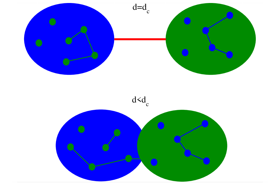
Figure 4: Pictorial representation of the phase-ordering process at $d=d_{c}$ (upper part) or $d<d_{c}$ (lower part). The blue and green regions are domains with spins up and down. The red line connecting them for $d=d_{c}$ is a red bond. See the text for a thorough explanation of the meaning of this sketch.

The fact that the exponent $a(d)$ must depend on $d$ is suggested by an argument according to which $a(d_{c})=1$, which is very different from $a(0)=0.178$. The argument is the following. Right at $d=d_{c}$ the network of the $J_{ij}$’s is a percolation structure. It is well known that such a fractal is characterised by the presence of so-called red bonds, namely bonds whose removal results in the disconnection of the network. This geometry is pictorially sketched in the upper part of Fig. 4. It is also known Burioni06 ; Burioni07 ; Burioni13 ; Corberi15 that, during phase-ordering kinetics at low temperatures on such a structure, interfaces between domains of opposite spins are located, with large probability, on the red bonds, where they get pinned for a very long time $\tau_{pin}$. Indeed, after depinning they quickly travel in a time $\tau_{move}\ll\tau_{pin}$ towards the next red bond. Since $\tau_{pin}/\tau_{move}\to\infty$ for $T_{f}\to 0$, in the low-temperature limit configurations in which the interface is located away from a red bond can be neglected if one is interested in the typical (average) configurations of the system at a generic time. In Fig. 4 the blue region on the left represents a group of, say, up spins, and the green region is a group of down spins. Inside such regions small islands of reversed spins can be present, and we draw them schematically by circles that can be connected among them (this is rendered by lines). The two large regions (blue and green) are linked by a red bond where the interface is located. Clearly i) the two blobs correspond to domains of aligned spins (possibly with thermal fluctuations in their interiors) and hence their size is of order $R$ and ii) the size ${\cal R}$ of the percolation cluster cannot be larger than the size $R$ of the domains because, in order to do that, the (say) left region should be connected through the red bond to some down spin inside the right region, but in this case the interface would not be located on the red bond. This implies that $R$ and ${\cal R}$ coincide and hence $a(d_{c})=1$. Notice that the situation is very different for $d<d_{c}$, where red bonds do not exist and the two domains are now connected by a number of order $R$ of links instead that by a single red bond, as represented in the lower part of the figure. In this case the percolation cluster can extend beyond $R$. For instance the down spins of the right domain could be connected to some of the islands of reversed spins inside the up domain, as shown in the figure. In this configuration the size $R$ of the correlated domains remains of the order of the typical size of the two blobs, but ${\cal R}$ can extend much beyond $R$.

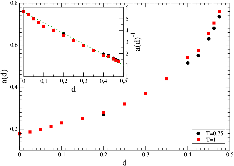
Figure 5: The exponent $a(d)$ against $d$, for $T_{f}=0.75$ and $T_{f}=1$ (see the key). In the inset we plot $a(d)^{-1}$ against $d$. The dotted green line represents $a(d)^{-1}=a(0)^{-1}-cd$, with $c=2(a(0)^{-1}-1)$.

The dependence of $a$ on $d$ is shown in Fig. 5 for two temperatures. From the comparison between these two cases one concludes that $a(d)$ is rather independent of $T_{f}$. These results imply that the formation of a spanning percolative cluster occurs at progressively larger values of $R$ as $d$ is increased. In other words, dilution slows down this process. Moreover, data show that the result of the previous argument, namely $a(1)=1$, is consistent with the numerical outcome. Let us mention that in Ref. Blanchard14 it was conjectured that, on deterministic lattices, $a\propto n_{c}^{-1}$, where $n_{c}$ is the average coordination number of the network. Since in our diluted case $n_{c}(d)=n_{c}(0)(1-d)$, a blind extension of the conjecture above to the random lattice at hand would result in the linear behaviour $a(d)^{-1}\propto n_{c}(0)(1-d)$. Although this form does not strictly describe the data, nevertheless, a linear decrease of $a(d)^{-1}$ with $d$ is neatly observed. Indeed, in the inset of Fig. 5 one sees that a behaviour of the form $a(d)^{-1}=a(0)^{-1}-cd$ (dotted greed line), where $c=2(a(0)^{-1}-1)$ is a constant, is well consistent with the numerical results.

The next quantity we consider is the averaged squared winding angle of the spin cluster interfaces. Its behaviour is exactly known in $2d$ critical percolation at $p=p_{c}$ Duplantier ; Wilson , where one has

$$\langle\theta^{2}_{perc}(r,r_{0})\rangle=a+K\ln\left(\frac{r}{r_{0}}\right)\,.$$ (7)

$a$ is a non-universal constant and $r_{0}$ is the lattice spacing. Beyond percolation theory, Eq. (7) is valid for the winding angle of a self similar interface, the fractal dimension of which, $D$, is related to $K$ by $D=4/(4-K)$. $\langle\theta^{2}\rangle$ was measured on the interfaces of the phase-ordering domains in the clean Ising model in Corberi17 . It was found that the form (7) is obeyed, with $R(t,0)$ playing the role of $r_{0}$, and with two different values of $K$ on scales $r\ll R(t,0)$ and $r\gg R(t,0)$. For $r\ll R(t,0)$ one probes the geometrical properties of the interfaces of the correlated domains. Since these are compact objects with a regular interface one has $D=1$, and hence $K=0$ nota . On the other hand, for $r\gg R(t,0)$ the fractal nature of the interface of the percolating structure emerges, leading to $K=K_{perc}$. This can be seen in Fig. 6 by looking at the curve with $d=0$. In the case of the RFIM and the RBIM, once the data for the winding angle are plotted against $r/R$, one finds a perfect superposition of the curves for the disordered models with those of the clean case Corberi17 . This is similar to what was observed for the crossing probabilities and is, again, due to the superuniversality property.

Let us now consider the case with dilution. The main difference with the behaviour of the IM, RFIM and RBIM is that in the regime $r\ll R(t,d)$ one finds $K=K(d)$, with $K(d)$ an increasing function of $d$ (see the inset of Fig. 6). This means that the interfaces of the correlated domains which are growing are fractal.

The following argument suggests that for $r\ll R(t,d)$, $K(d_{c})=1$. Indeed, up to now, we have considered the so-called spin or geometrical clusters built by connecting nearest neighbouring sites occupied by the same spin value. For the bond percolation corresponding to the dilution $d=d_{c}$, the natural objects to consider are the Fortuin-Kasteleyn (FK) clusters FK for which the $K$ of their interface is $K=K^{\rm FK}_{int}=12/7$ and, therefore, the fractal dimension is $D^{\rm FK}_{int}=4/(4-K^{\rm FK}_{int})=7/4$. However, we are studying here the interfaces of the spin clusters Delfino and we are therefore measuring a $K$ (and its associated fractal dimension) that will not take this value. In fact, we are measuring a $K$ that has been shown to be equal to the one of the external perimeter of the FK clusters Duplantier2 ; Adams . For any critical $Q$ state Potts model, and critical percolation is a particular case with $Q=1$, the fractal dimensions of the FK clusters interface, $D^{\rm FK}_{int}$, and the one of the FK clusters external perimeter, $D^{\rm FK}_{extp}$, are related by the equation $(D^{\rm FK}_{int}-1)(D^{\rm FK}_{extp}-1)=1/4$ Duplantier2 . Replacing $D^{\rm FK}_{int}=7/4$ one readily finds $D^{\rm FK}_{extp}=4/3$ and $K^{\rm FK}_{extp}=K(d_{c})=1$. We see in the inset of Fig. 6 that, indeed, data are consistent with $K(d_{c})=1$ which then implies that the fractal dimension of the interfaces is $D=4/3$ at $d=d_{c}$. Notice also that $K(d)$ increases in an approximately linear way with $d$, a fact for which we have no explanation.

In the large distance regime, for $r\gg R(t,d)$, one recovers the slope $K=K_{perc}=12/7$, that is independent of $d$ and the same as the one observed for the clean system, which shows quite convincingly that the geometry of the clusters of aligned spins on such large scales is the one of percolation.

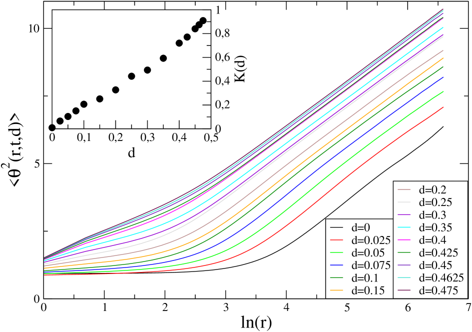
Figure 6: The averaged squared winding angle $\langle\theta^{2}(r,t,d)\rangle$ is plotted against $\ln r$ for different values of the dilution $d$ (see the key). For each $d$ the data refer to the longest simulated time (this time is $t=1218$, 1218, 939, 1125, 939, 1680, 1681, 939, 1865, 2142, 1681, 2603, 2603, 2603, 2603 for $d=0,0.25,\dots,0.475$, respectively). In the inset the slope $K(d)$ of the small $r$ part of the curves is plotted against $d$. This quantity was computed by a linear fitting of the curves in the range $0.6\leq\ln r\leq 1.4$.

The behaviour of $\langle\theta^{2}\rangle$ for a fixed value of $d$ and different times is shown in the inset of Fig. 7 (a similar behaviour is obtained for all values of $d$ below $d_{c}$). Here we see that the value $r_{cross}$ of $r$ where there is a change in the slope of the curve increases as time elapses. Since $R(t,d)^{D}$ is a natural length associated to the fractal character of the interfaces we assume, as in Ref. Tartaglia18 , that $r_{cross}\sim R(t,d)^{D}$. Hence, recalling the discussion above, we argue that $\langle\theta^{2}\rangle$ obeys the following form

$$\langle\theta^{2}(r,t,d)\rangle=\left\{\begin{array}[]{ll}a(d)+K(d)\ln r&\qquad\mbox{for}\quad r\ll R(t,d)^{D}\;,\\ a(d)+K(d)\ln[R(t,d)^{D}]+K_{perc}\ln\left[\frac{r}{R(t,d)^{D}}\right]&\qquad\mbox{for}\quad r\gg R(t,d)^{D}\;.\end{array}\right.$$ (8)

This formula simply expresses the fact that the squared winding angle has two linear behaviours with slopes $K(d)$ and $K_{perc}$ which match at $r=R(t,d)^{D}$. Clearly, for $r\simeq R(t,d)^{D}$, $\langle\theta^{2}\rangle$ interpolates smoothly between the two limiting forms of Eq. (8). According to this conjecture one should have

$$\langle\theta^{2}(r,t,d)\rangle-K(d)\ln[R(t,d)^{D}]=f_{d}\left[\frac{r}{R(t,d)^{D}}\right]$$ (9)

with

$$f_{d}(x)=\left\{\begin{array}[]{ll}K(d)\;\ln x&\qquad\mbox{for}\quad x\ll 1\;,\\ K_{perc}\,\ln x&\qquad\mbox{for}\quad x\gg 1\;.\end{array}\right.$$ (10)

Equation (9) implies that plotting $\langle\theta^{2}(r,t,d)\rangle-K(d)\ln[R(t,d)^{D}]$ as a function of $r/R(t,d)^{D}$ for each value of $d$ should lead to data collapse of the curves at different times on the mastercurve with the properties (10). We check this feature in Fig. 7. Here, in the main part of the figure, we find a very good collapse of the curves, and the limiting behaviour of the mastercurve agrees with those in Eq. (10). Similar results are found for any value of $d$. Notice, however, that the mastercurve $f_{d}(x)$ depends on $d$. As a last remark, let us point out that the non trivial fractal character of the interfaces due to dilution, which gives rise to $K=K(d)$, is observed up to scales as large as $R^{D}>R$. This is at variance with possible effects due to thermal roughening, see the discussion in nota , which are confined to very short length scales. It is, instead, similar to what we observed in two other cases: (i) the quench to a critical point, in particular, the one of the clean Ising model Blanchard12 and (ii) the dynamics of the voter model Tartaglia15 ; Tartaglia18 .

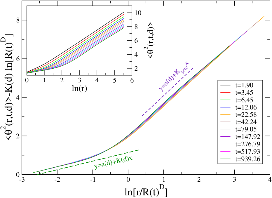
Figure 7: In the inset $\langle\theta^{2}(r,t,d)\rangle$ evaluated at different times $t$ (see the key) is plotted against $\ln r$ for a system with $d=0.25$. In the main part of the figure, for the same sets of data of the inset (but only for $t\geq 22.58$, in order to focus on the asymptotic behaviour), we plot the quantity $\langle\theta^{2}(r,t,d)\rangle-K(d)\ln[R(t,d)^{D}]$ (see Eq. (9)) against $\ln[r/R(t,d)^{D}]$. The dashed green and violet lines are the linear behaviours with slopes $K(d)$ and $K_{perc}$, respectively.

Let us now turn to the properties of the pair connectedness defined in Eq. (5). For large distances $r$, random percolation theory at $p=p_{c}$ in a $d=2$ infinite system gives Stauffer ; Saberi ; Christensen

$$C_{perc}(r,r_{0})\sim\left(\frac{r}{r_{0}}\right)^{-2\Delta}$$ (11)

where $r_{0}$ is a microscopic length, e.g. the lattice spacing, and with the critical exponent $\Delta=5/48$. Since we are considering a system with periodic boundary conditions which corresponds to a torus, then for a system of finite size $L$, the form (11) contains some correction of order ${r/L}$ which will cause an upward bending of the curve with respect to the algebraic behaviour Corberi17 .

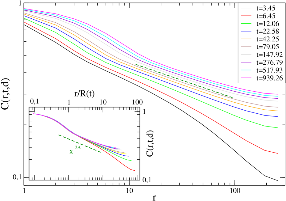
Figure 8: The pair connectedness function $C(r,t,d)$ is plotted against $r$ at different times (see the key) for $d=0.25$. The dashed green line is the algebraic behaviour $x^{-2\Delta}$ of critical percolation Eq. (11). In the inset the same data (except the one at the earliest time) are plotted against $r/R(t)$.

In Fig. 8 we plot the pair connectedness against $r$ measured in the coarsening stage of the diluted model with $d=0.25$ at different times (similar results are found for other values of $d$). Qualitatively, the behaviour of these curves is analogous to the one that was found in the clean case and in the RFIM and RBIM Corberi17 . A first observation is that, since the number of domains decreases during coarsening, the probability that two randomly chosen points belong to the same cluster, namely the area $\sum_{r}C(r,t,d)$ below the curves, increases in time. Secondly, the behaviour of the pair connectedness is different for $t\ll t_{p}$ and $t\gg t_{p}$. Indeed, for $t\gg t_{p}$ the percolating structure has established for $r>R(t,d)$, whereas it is not well developed for $t\ll t_{p}$. This is reflected by the fact that the slope $r^{-2\Delta}$ is clearly observed for sufficiently large values of $r$ in the curves for $t\gtrsim 42.25$, whereas a faster decay occurs at early times. Let us notice also that the $r^{-2\Delta}$ behaviour is spoiled at very large $r$ or more precisely for finite values of ${r\over L}$ since our simulations are done on a torus geometry. For $t\gg t_{p}$ the pair connectedness crosses over between a short distance behaviour, for $r\ll R(t,d)$, where the properties inside the correlation distance are tested, to the large distance behaviour, $r\gg R(t,d)$, where there is no correlation and the percolative structure emerges. In this regime one expects Eq. (11) to hold, with $r_{0}=R(t,d)$ Corberi17 . This behaviour can be summarised in the scaling form

$$C(r,t,d)={\cal C}_{d}\left(\frac{r}{R(t,d)}\right),$$ (12)

valid for an infinite system, with

$${\cal C}_{d}(x)\sim x^{-2\Delta}$$ (13)

for $x\gg 1$. In the inset of Fig. 8 we plot the same data of the main figure against $r/R(t,d)$, in order to check the accuracy of Eqs. (12) and (13). In this plot one clearly sees that the curves change behaviour around $r/R(t,d)=1$. For $r/R(t,d)<1$ one has a good collapse at all times, even for $t<t_{p}$. This is because the growth of correlations on scales $r<R(t,d)$ is independent of the establishment of percolation on scales much larger than $R(t,d)$. For $r/R(t,d)>1$ one expects data collapse only for $t>t_{p}$ and in a range of $r$ free from finite size effects. This is indeed observed in the inset of Fig. 8. Notice that the finite size effects limit the range over which collapse is observed to smaller and smaller values of $r/R(t,d)$ in this kind of plot. Let us also mention that one can collapse the curves for $r/R(t,d)>1$ with a different rescaling Corberi17 . Indeed, finite size scaling implies that in a system of size $L$ the form (13) changes into ${\cal C}_{d}(x)\simeq x^{-2\Delta}\Lambda(r/L)$, where $\Lambda(x)$ is a scaling function describing the finite size properties. Hence, by plotting $[r/R(t,d)]^{2\Delta}C(r,t,d)$ against $r/L$ one should get data collapse for $r\gg R(t,d)$ at different times and for different system sizes. This is shown to be true in the inset of Fig. 9 (here, since the system size $L$ is fixed we plot simply against $r$).

A final important remark is the fact that, as already observed for the squared winding angle, the scaling function ${\cal C}_{d}$ does actually depend on $d$. This implies that superuniversality does not hold for this quantities. We show this in the main part of Fig. 9, where we plot $C(r,t_{max},d)$, where $t_{max}$ is the longest simulated time, against $r/R(t,d)$ (this is the best determination of ${\cal C}_{d}$ apart from finite size effects), for $d=0.05$, $d=0.25$ and $d=0.4$. This figure shows a marked difference between the scaling functions as $d$ is varied, despite a certain similarity among the curves.

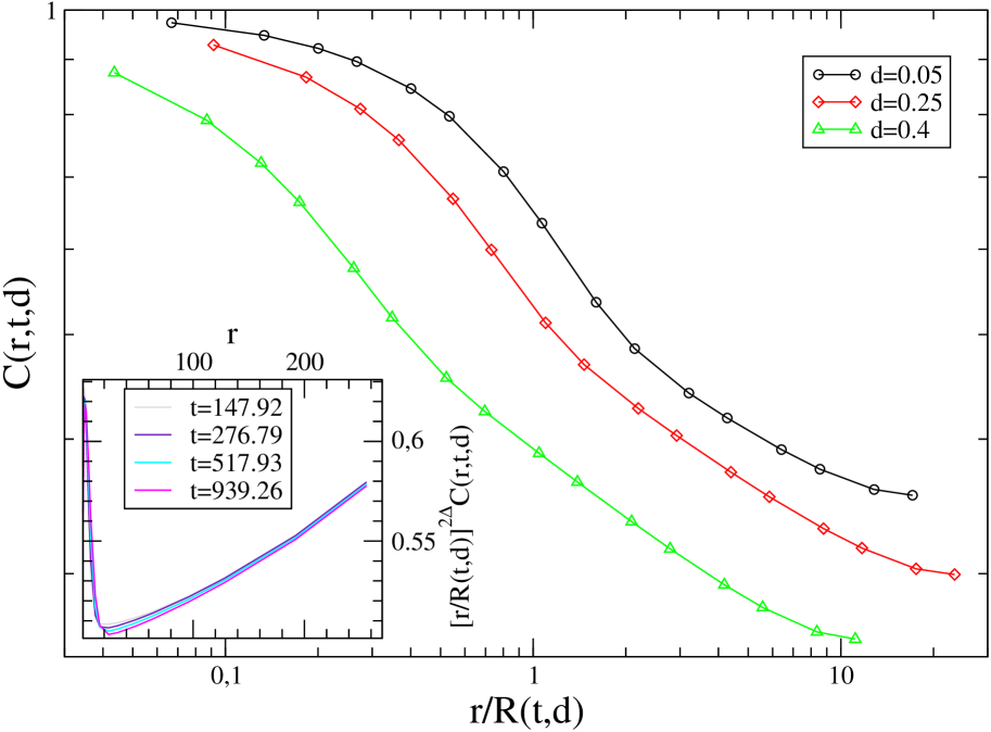
Figure 9: The pair connectedness function $C(r,t,d)$ at the longest simulated time is plotted against $r/R(t,d)$ for $d=0.05$, $d=0.25$, and $d=0.4$ (see the key). In the inset, the data for $d=0.25$ are presented by plotting $[r/R(t,d)]^{2\Delta}C(r,t,d)$ against $r$, in order to collapse the finite size part of the curves.

IV Conclusions

In this paper we studied numerically the phase-ordering kinetics of the two-dimensional BDIM with Glauber transition rates, i.e. with non conserved order parameter dynamics, quenched from an equilibrium initial state at infinite temperature to a low temperature $T_{f}$. The growth law and other dynamical properties of this system, with similar choices of the model parameters, had been considered in Corberi15 , and in the three dimensional case in Corberi15b . The closely related model with site dilution was analysed in Corberi13 . In all these studies it was argued that the growth law is logarithmically slow for any $0<d<d_{c}$. For the limiting values of the dilution, instead, the system behaves differently. With $d=0$ there is no disorder and the usual algebraic law $R(t,0)\sim t^{1/2}$ holds. The case $d=d_{c}$, instead, is much less trivial, because the fractal character of the bond network (or site network in the case of site dilution), results in an algebraic growth of $R(t,d_{c})$ regulated by a temperature dependent exponent.

In this paper we continue the study of the coarsening kinetics of diluted systems focusing on the characterisation of the geometrical properties of the dynamic configurations of the quenched BDIM on the square lattice. Beyond addressing some of the properties of the domains and their boundaries, an issue that has been longly discussed in system with quenched disorder  Nattermann87 ; Fisher86 ; Kardar87 ; Halpin89 ; Huse85 ; Kardar85 ; Huse85b ; Corberi16 ; Corberi16b , we also investigate the geometrical properties on scales much larger than those of the correlated regions, following a more recent research line aimed at the comprehension and characterisation of the emerging percolative features.

We find that domain walls are fractal interfaces with a Hausdorff dimension that depends continuously on the dilution parameter $d$. This is at variance with what is expected for the RBIM Nattermann87 ; Fisher86 ; Kardar87 ; Halpin89 where the roughness of the interfaces due to the bond randomness is expected to be described by a unique exponent, irrespective of the amount of disorder. This is at odds with the fact the the BDIM is an instance of a system with bond disorder, as the RBIM, and one could have expected the same exponent in the two cases (and independently of the strength of disorder) since both belong to the “interface disorder” family of systems.

Our results confirm the development, on scales larger than $R(t,d)$, of an uncorrelated object with the topology of a critical percolation cluster. The size $R_{p}(t,d)$ of this object grows faster (for any $d<d_{c}$) than $R(t,d)$, in a way which is regulated by a dilution-dependent exponent. Interestingly, right at $d_{c}$, $R_{p}(t,d)\propto R(t,d)$, a fact which is possibly due to the percolative nature of the bond network itself.

This study allows us to discuss the issue of superuniversality in this system. Our results clearly indicate that, at variance with what was found for the RFIM and the RBIM considered in Refs. Corberi17 ; Insalata18 , this property is not obeyed (at least not fully) in the BDIM. This conclusion is reached by the recognition that geometrical features such as $D$ and $R_{p}$ show a continuous dependence on the amount of dilution. Indeed, our study shows that physical quantities such as, for instance, the crossing probabilities, the averaged squared winding angle and the pair connectedness function obey some instance of scaling form, but with scaling functions that are themselves dependent on the dilution parameter $d$. We expect similar results to hold for the related model with site dilution.

Acknowledgements L. F. C. is a member of Institut Universitaire de France. We warmly thank our former students T. Blanchard and A. Tartaglia for several years of collaborative research on these topics. F.C. acknowledges financial support by MIUR project PRIN2015K7KK8L.

References

- (1) A. J. Bray, Adv. Phys. 43, 357 (1994).
- (2) Kinetics of Phase Transitions, edited by S. Puri and V. Wadhawan, (CRC Press, Boca Raton, 2009).
- (3) F. Corberi, L. F. Cugliandolo, and H. Yoshino, Growing length scales in aging systems in: Dynamical heterogeneities in glasses, colloids, and granular media, edited by L. Berthier, G. Biroli, J.-P. Bouchaud, L. Cipeletti, and W. van Saarloos (Oxford University Press, Oxford, 2010).
- (4) F. Corberi, E. Lippiello, and M. Zannetti, Phys. Rev. E 78, 011109 (2008).
- (5) J. J. Arenzon, A. J. Bray, L. F. Cugliandolo, and A. Sicilia, Phys. Rev. Lett. 98, 145701 (2007).
- (6) A. Sicilia, J. J. Arenzon, A. J. Bray, and L. F. Cugliandolo, Phys. Rev. E 76, 061116 (2007).
- (7) A. Sicilia, J. J. Arenzon, A. J. Bray, and L. F. Cugliandolo, EPL 82, 10001 (2008).
- (8) A. Sicilia, Y. Sarrazin, J. J. Arenzon, A. J. Bray, and L. F. Cugliandolo, Phys. Rev. E 80, 031121 (2009).
- (9) T. Blanchard, L. F. Cugliandolo, and M. Picco, J. Stat. Mech. P05026 (2012).
- (10) T. Blanchard, F. Corberi, L. F. Cugliandolo, and M. Picco, EPL 106, 66001 (2014).
- (11) A. Tartaglia, L. F. Cugliandolo, and M. Picco, Phys. Rev. E 92, 042109 (2015).
- (12) A. Tartaglia, L. F. Cugliandolo, and M. Picco, Europhys. Lett. 116, 26001 (2016).
- (13) T. Blanchard, A. Tartaglia, L. F. Cugliandolo, and M. Picco, J. Stat. Mech. 113201 (2017).
- (14) F. Corberi, L. F. Cugliandolo, F. Insalata, and M. Picco, Phys. Rev. E 95, 022101 (2017).
- (15) F. Insalata, F. Corberi, L. F. Cugliandolo, and M. Picco, J. Phys.: Conf. Ser. 956, 012018 (2018).
- (16) A. Tartaglia, L. F. Cugliandolo, and M. Picco, J. Stat. Mech. 083202 (2018).
- (17) J. Cardy and R. M. Ziff, J. Stat. Phys. 110, 1 (2003).
- (18) K. Barros, P. L. Krapivsky, and S. Redner, Phys. Rev. E 80, 040101 (2009).
- (19) J. Olejarz, P. L. Krapivsky, and S. Redner, Phys. Rev. Lett. 109, 195702 (2012).
- (20) T. Blanchard and M. Picco, Phys. Rev. E 88, 032131 (2013).
- (21) J. H. Oh, and D. Choi, Phys. Rev. B 33, 3448 (1986).
- (22) E. Oguz, A. Chakrabarti, R. Toral, and J. D. Gunton, Phys. Rev. B 42, 704 (1990).
- (23) A. J. Bray and K. Humayun, J. Phys. A 24 , L1185 (1991).
- (24) S. Puri, D. Chowdhury, and N. Parekh, J. Phys. A 24, L1087 (1991).
- (25) S. Puri and N. Parekh, J. Phys. A 26, 2777 (1993).
- (26) M. Rao and A. Chakrabarti, Phys. Rev. E 48, R25(R) (1993).
- (27) M. Rao and A. Chakrabarti, Phys. Rev. Lett. 71, 3501 (1993).
- (28) E. Oguz, J. Phys. A 27, 2985 (1994).
- (29) M. F. Gyure, S. T. Harrington, R. Strilka, and H. E. Stanley, Phys. Rev. E 52, 4632 (1995).
- (30) D. S. Fisher, P. Le Doussal, and C. Monthus, Phys. Rev. Lett. 80, 3539 (1998).
- (31) D. S. Fisher, P. Le Doussal, and C. Monthus, Phys. Rev. E 64, 066107 (2001).
- (32) F. Corberi, A. de Candia, E. Lippiello, and M. Zannetti, Phys. Rev. E 65, 046114 (2002).
- (33) E. Lippiello, A. Mukherjee, S. Puri, and M. Zannetti, Europhys. Lett. 90, 46006 (2010).
- (34) R. Paul, S. Puri, and H. Rieger, Europhys. Lett. 68, 881 (2004).
- (35) R. Paul, S. Puri, and H. Rieger, Phys. Rev. E 71, 061109 (2005).
- (36) M. Henkel and M. Pleimling, Europhys. Lett. 76, 561 (2006).
- (37) R. Paul, G. Schehr, and H. Rieger, Phys. Rev. E 75, 030104(R) (2007).
- (38) C. Aron, C. Chamon, L. F. Cugliandolo, and M. Picco, J. Stat. Mech. P05016 (2008).
- (39) M. Henkel and M. Pleimling, Phys. Rev. B 78, 224419 (2008).
- (40) H. Park and M. Pleimling, Phys. Rev. B 82, 144406 (2010).
- (41) F. Corberi, E. Lippiello, A. Mukherjee, S. Puri, and M. Zannetti, J. Stat. Mech. P03016 (2011).
- (42) F. Corberi, E. Lippiello, A. Mukherjee, S. Puri, and M. Zannetti, Phys. Rev. E 85, 021141 (2012).
- (43) F. Corberi, R. Burioni, E. Lippiello, A. Vezzani, and M. Zannetti, Phys. Rev. E 91, 062122 (2015).
- (44) H. Ikeda, Y. Endoh, and S. Itoh, Phys. Rev. Lett. 64, 1266 (1990).
- (45) A. G. Schins, A. F. M. Arts, and H. W. de Wijn, Phys. Rev. Lett. 70, 2340 (1993).
- (46) D. K. Shenoy, J. V. Selinger, K. A. Grüneberg, J. Naciri, and R. Shashidhar, Phys. Rev. Lett. 82, 1716 (1999).
- (47) V. Likodimos, M. Labardi, and M. Allegrini, Phys. Rev. B 61, 14440 (2000).
- (48) V. Likodimos, M. Labardi, X. K. Orlik, L. Pardi, M. Allegrini, S. Emonin, and O. Marti, Phys. Rev. B 63, 064104 (2001).
- (49) F. Corberi, E. Lippiello, A. Mukherjee, S. Puri, and M. Zannetti, Phys. Rev. E 88, 042129 (2013).
- (50) D. S. Fisher and D. A. Huse, Phys. Rev. B 38, 373 (1988).
- (51) D. Stauffer and A. Aharony, Introduction to Percolation Theory (Taylor and Francis, London, 1994).
- (52) K. Christensen, Percolation Theory (Imperial College Press, London, 2002).
- (53) A. A. Saberi, Phys. Rep. 578, 1 (2015).
- (54) F. Corberi, Comptes rendus - Physique 16, 332 (2015).
- (55) S. Puri and N. Parekh, J. Phys. A 25, 4127 (1992).
- (56) A. J. Bray and K. Humayun, J. Phys. A 24, L1185 (1991).
- (57) B. Biswal, S. Puri, and D. Chowdhury, Physica A 229, 72 (1996).
- (58) C. Castellano, F. Corberi, U. Marini Bettolo Marconi, and A. Petri, Journal de Physique IV 8,93 (1998).
- (59) F. Corberi, E. Lippiello, and M. Zannetti, J. Stat. Mech. P10001 (2015).
- (60) Y. Imry and S.-k. Ma, Phys. Rev. Lett. 35, 1399 (1975).
- (61) J. L. Iguain, S. Bustingorry, A. B. Kolton, and L. F. Cugliandolo, Phys. Rev. B 80, 094201 (2009).
- (62) H. Pinson, J. Stat. Phys. 75, 1167 (1994).
- (63) B. Duplantier and H. Saleur, Phys. Rev. Lett. 60, 2343 (1988).
- (64) B. Wieland and D. B. Wilson, Phys. Rev. E 68, 056101 (2003).
- (65) F. Corberi, E. Lippiello and M. Zannetti, J. Stat. Mech. P10001 (2015).
- (66) R. Burioni, D. Cassi, F. Corberi, and A. Vezzani, Phys. Rev. Lett. 96, 235701 (2006).
- (67) R. Burioni, D. Cassi, F. Corberi, and A. Vezzani, Phys. Rev. E 75, 011113 (2007).
- (68) R. Burioni, F. Corberi, and A. Vezzani, Phys. Rev. E 87, 032160 (2013).
- (69) It should be mentioned that, in principle, if the quench is made to a finite temperature , roughening of interfaces takes place and, on scales of the order of the roughening length , this should result in . However, since in the roughness of the interface is of order Corberi2008 ; Corberi16 , where is a constant which vanishes for , this effect would produce on scales so small that the effect cannot be observed in our data (see Fig. 6).
- (70) P.W. Kasteleyn and E.M. Fortuin, J. Phys. Soc. Jpn. Suppl. 26 (1969) 11; Physica 57 (1972) 536.
- (71) G. Delfino, M. Picco, R. Santachiara, and J. Viti, J. Stat. Mech. (2013) P11011.
- (72) B. Duplantier, Phys. Rev. Lett. 84, 1363 (2000).
- (73) D. A. Adams, L. M. Sander, and R. M. Ziff, J. Stat. Mech. (2010) P03004.
- (74) F. Corberi, E. Lippiello, and M. Zannetti, Europhys. Lett. 116, 10006 (2016).
- (75) T. Nattermann, Europhys. Lett. 4, 1241 (1987).
- (76) M. E. Fisher, J. Chem. Soc., Faraday Trans. 82, 1569 (1986).
- (77) M. Kardar, J. Appl. Phys. 61, 3601 (1987).
- (78) T. Halpin-Healy, Phys. Rev. Lett. 62, 442 (1989); Phys. Rev. A 42, 711 (1990).
- (79) D. A. Huse and C. L. Henley, Phys. Rev. Lett. 54, 2708 (1985).
- (80) M. Kardar, Phys. Rev. Lett. 55, 2923 (1985).
- (81) D. A. Huse, C. L. Henley, and D. S. Fisher, Phys. Rev. Lett. 55, 2924 (1985).
- (82) F. Corberi, E. Lippiello, and M. Zannetti, J. Phys. A: Math. Theor. 49, 185001 (2016).
- (83) M. P. O. Loureiro, J. J. Arenzon, L. F. Cugliandolo, and A. Sicilia, Phys. Rev. E 81, 021129 (2010).
- (84) T. Iwai, and H. Hayakawa, J. Phys. Soc. Japon 62, 1583 (1993).
- (85) W. Selke, L. N. Shchur, and O. A. Vasilyev, Physica A 259, 388 (1998).
- (86) H.-O. Heuer, Phys. Rev. B 45 (1992) 5691.
- (87) J.-K. Kim, and A. Patrascioiu, Phys. Rev. Lett. 72 (1994) 2785.
- (88) R. Stinchcombe, in: Phase Transitions and Critical Phenomena, vol.7, C. Domb and J. L. Lebowitz, eds., (Academic Press, New York, 1983).