Magnetic Phases of Frustrated Ferromagnetic Spin-Trimer System Gd₃Ru₄Al₁₂ With a Distorted Kagome Lattice Structure

Abstract

The magnetization and specific heat measurements have been performed on single-crystalline Gd₃Ru₄Al₁₂, wherein magnetic Gd–Al layers with a distorted Kagome lattice structure and non magnetic Ru–Al layers are stacked alternately along the $c$ axis. A recent investigation has indicated that the distorted Kagome lattice structure of Gd–Al layers effectively translates into an antiferromagnetic triangular lattice in association with ferromagnetic spin trimerization at low temperatures. We investigate the successive phase transitions and peculiar features of magnetic phases on this effective triangular lattice of spin trimers. This spin system is found to be a $XY$ like Heisenberg model. The magnetic phase diagrams indicate the existence of frustration and ${\bm{Z}_{2}}$ degeneracy. The magnetization and specific heat imply the successive phase transitions with partial disorder and a T-shaped spin structure in the ground state.

I Introduction

Metallic $4f$ frustrated spin systems often exhibit peculiar features at low temperatures. Ternary intermetallic compounds RE₃Ru₄Al₁₂ (RE: rare earth) crystallize in a hexagonal structure of Gd₃Ru₄Al₁₂-type, which belongs to the space group $P6_{3}/mmc$ Niermann2002 . In this crystal, magnetic RE-Al layers and non-magnetic Ru-Al layers stack alternately along the $c$ axis [Figs. 1 (a) and (b)] VESTA . As shown in Fig. 1 (c), the RE ions form a distorted kagome lattice or a breathing kogome lattice composed of two different sized regular triangles and unequal sided hexagons. RE₃Ru₄Al₁₂ has been investigated intensively in recent years because of the various phenomena it shows at low temperatures. La₃Ru₄Al₁₂ is Pauli paramagnetic (PM) and Pr₃Ru₄Al₁₂ and Nd₃Ru₄Al₁₂ are ferromagnetic (FM) Ge2012 ; Ge2014 ; Troc2012 ; Gorbunov2016 . Ce₃Ru₄Al₁₂ is thought to be a valence fluctuation system Niermann2002 . When the RE sites are replaced by heavy RE ions, RE₃Ru₄Al₁₂ shows antiferromagnetic (AFM) properties. Yb₃Ru₄Al₁₂ is an $XY$-antiferromagnet with Néel order at $T_{\rm N}=1.5$ K Nakamura2014 ; Nakamura2015 . This compound is a heavy fermion system with enhanced Sommerfeld coefficients $\gamma_{0}=120$ mJ/(K² Yb-mol. Dy₃Ru₄Al₁₂ is an AFM compound with $T_{\rm N}=7$ K, which has a noncollinear spin structure Gorbunov2014 . Regardless of the long range AFM ordering, this compound shows a large $\gamma_{0}$ value of about 500 mJ/(K² Dy-mol) in the temperature range 7-20 K. Gorbunov et al. attributed this large $\gamma_{0}$ value to spin fluctuations induced in the Ru 4$d$ electrons by the exchange field acting from Dy 4$f$ electrons Gorbunov2014 . Chanragiri et al. have found characteristics of spin glass like dynamics in Dy₃Ru₄Al₁₂ in AFM phase which indicates a complex ground state under the influence of geometrical frustration Chandragiri2016 .

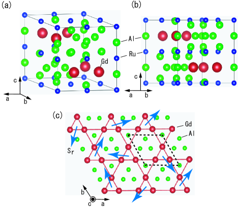
Figure 1: (Color online) (a) Structure of Gd₃Ru₄Al₁₂ Niermann2002 ; VESTA . The red (large), blue (small) and light green (middle) spheres denote Gd, Ru and Al ions, respectively. (b) Structure projected parallel to the $ab$ plane. (c) A Gd–Al layer projected parallel to the $c$ axis. The red (larger) and light green (smaller) spheres denote Gd and Al ions, respectively. Bonds are drawn between the nearest neighbor and next nearest neighbor Gd ions. The blue arrows indicate resultant spin $\bm{S}_{r}$ ($S_{r}=21/2$) on the FM trimers. The broken rhombus indicates a unit cell.

In 2016, Chandragiri et al. reported the magnetic behavior of poly-crystalline Gd₃Ru₄Al₁₂, whose magnetic susceptibility follows the Curie–Weiss law above 200 K and whose Curie–Weiss temperature ($\theta_{p}$) has been estimated to be +80 K Chandragiri2016_2 . The magnetic susceptibility begins to increase rapidly with temperature decreasing below 50 K, which implies the development of a FM correlation between the spins. However, it exhibits a sharp peak at 18.5 K, indicating AFM order. The magnetic specific heat exhibits a broad maximum around 50 K, suggesting a glassy ground state. On the other hand, the magnetic susceptibility exhibits a very small difference under zero field cool (ZFC) and field cool (FC) conditions. The behavior of the magnetic susceptibility under magnetic fields is mimics that expected for the Griffiths phase Griffiths1969 . Very recently, Nakamura et al. investigated the low-temperature magnetic and thermodynamic properties of single-crystalline Gd₃Ru₄Al₁₂ Nakamura2018 . They proposed that ferromagnetic (FM) spin trimers are formed on small Gd-triangles at low temperatures, and that the distorted Kagome lattice of Gd₃Ru₄Al₁₂ effectively transforms into an antiferromagnetic triangular lattice (AFMTL) at low temperatures. The blue arrows $\bm{S_{r}}$ in Fig. 1 denote the resultant spin ($S_{r}=21/2$) formed by the Ruderman–Kittel–Kasuya–Yosida (RKKY) interaction on the trimers. These $\bm{S_{r}}$’s begin to be formed around 150 K and are completed below 70 K. The binding energy is thought to be 184 K per Gd ion. On further decreasing temperature, Gd₃Ru₄Al₁₂ exhibit successive AFM phase transition at $T_{2}=18.6$ K and $T_{1}=17.5$ K. The magnetic entropy at $T_{2}=18.6$ K is only 40% of $R{\rm ln}8$, indicating spin frustration. Because binding energy is much higher than that at these transition temperatures, the FM trimers are probably stable even in the ordered phases.

The ground state and magnetic phase diagrams of two-dimensional (2D) AFMTL’s and three-dimensional (3D), or layered AFMTL’s of Heisenberg models and related models (Heisenberg-Ising and Heisenberg-$XY$ models) have been extensively investigated for long years from the view point of geometrical frustration Kawamura1998Review . On the other hand, the oscillatory features of the RKKY interaction lead to the frustration arising from the competition between the near and far-neighbor interactions, which induce the spin glass in random system and spiral magnets in periodic systems Kawamura1998Review . In the case of Gd₃Ru₄Al₁₂, the long range and oscillatory feature of the RKKY interaction also induces a geometrical frustration in association with the formation of FM trimers at low temperatures Nakamura2018 . The present paper addresses the spin structures in the ordered phases and magnetic phase diagrams of the layered frustrated spin trimer system Gd₃Ru₄Al₁₂ wherein the geometrical and the interaction-compete-type frustrations coexist. The $\bm{S_{r}}$ system in Gd₃Ru₄Al₁₂ is regarded as an AFMTL lattice of the Heisenberg model with a certain degree strong anisotropy and interlayer interactions at low temperatures. The long reaching range of the RKKY interaction may lead to some clear appearances of the geometrical frustration regardless of a slightly complicated geometrical structure of the distorted kagome lattice.

II Typical magnetic phase diagrams with weak anisotropy

The Hamiltonian of 2D Heisenberg model with weak anisotropy on AFMTL’s under the field is written as,

$$\mathscr{H}=J\sum_{i,j}{\bm{S}_{i}}{\bm{S}_{j}}-D\sum_{i}(S_{i}^{z})^{2}+g_{s}\mu_{\rm B}H_{z}\sum_{i}S_{i}^{z}.$$ (1)

Here, the first term on the right side denotes the exchange interaction, the second term denotes the local anisotropy at $i$ site, and the last term denotes the Zeeman energy. When $D$ is negative, the spin system is $XY$ like (easy plane type anisotropy), and when $D$ is positive, the spin system is Ising like (easy axis type anisotropy). Several theoretical investigations of frustrated AFMTL or layered AFMTL with anisotropy predict two successive phase transitions when $D>0$ at zero field MiyashitaKawamura1985 ; Miyashita1986 ; Kawamura1998Review . In this case, the spin component along the easy axis and the other spin components are ordered at distinct temperatures. In the case where the anisotropy is relatively strong, three successive phase transitions are expected Melchy2009 . On the other hand, when $D<0$, only single-phase transition is expected at zero field MiyashitaKawamura1985 ; Miyashita1986 ; Kawamura1998Review .

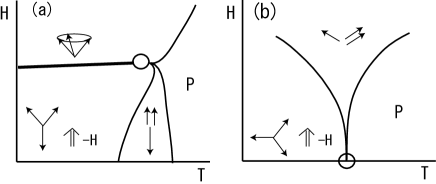
Figure 2: Schematic magnetic phase diagrams of frustrated layered AFMTL with weak anisotropic interaction Kawamura1990 ; Kawamura1998Review . (a) Easy axis type. The bold line indicates first-order transition and the open circle denotes a tetracritical point. Fields are directed along the easy axis. (b) Easy plane type. The open circle denotes a tetracritical point. Fields are directed parallel to the easy plane. The minus sign of ${\bm{H}}$ denotes that the magnetic moments are in the opposite directions of the spins.

The Hamiltonian of the layered Heisenberg model with weak anisotropy on AFMTL’s under the field is written as

$$\mathscr{H} =J\sum_{i,j}{\bm{S}_{i}}{\bm{S}_{j}}+J^{\prime}\sum_{i,j}{\bm{S}_{i}}{\bm{S}_{j}}-D\sum_{i}(S_{i}^{z})^{2}$$

$$\quad+g_{s}\mu_{\rm B}H_{z}\sum_{i}S_{i}^{z}.$$ (2)

Here, the first term on the right side indicates intralayer exchange interaction and the second term indicates interlayer exchange interaction. When the anisotropy is the easy axis type ($D>0$), two successive phase transitions are expected at zero field, similar to the 2D lattice Kawamura1990 ; Kawamura1998Review . We illustrate schematic phase diagrams in Fig. 2 according to these previous studies. In the IMT phase shown in Fig. 2 (a), only longitudinal spin component is ordered. The ground state is the noncolinear spin structure. This state translates to the umbrella structure at high fields in association with the first order phase transition when the field is applied along the easy axis. A tetracritical point is predicted at the high temperature end of the first order boundary. When $D<0$, only single-phase transition is expected at zero field, similar to 2D system, and this transition point becomes a tetracritical point due to $\bm{Z_{2}}$ degeneracy. CsNiCl₃ is known for a substance that shows a phase diagram such as that in Fig. 2 (a) Clark1972 ; Poirier1990 ; Backmann1993 ; Kadowaki1987 ; Maegawa1988 and CsMnBr₃ is for a substance that shows a diagram such as that in Fig. 2 (b) Gaulin1989 .

III Sample preparation and experimental method

We melted 3N-Gd, 3N-Ru, and 5N-Al in a tetra-arc furnace and pulled a single-crystal ingot. Considering evaporation loss, the initial weight of Al was increased by 1–2% in comparison to the stoichiometric amount. The obtained ingot was about 2–3 cm in length and 3 mm in diameter. We determined the crystal structure of the ingot by X-ray diffraction with crushed powder samples. The diffraction pattern was consistent with that of a previous report Niermann2002 . The lattice constants of Gd₃Ru₄Al₁₂ were obtained as 0.8778 nm for the $a$ axis and 0.9472 nm for the $c$ axis. The length of the side of the small regular triangle was 0.3698 nm and that of the large regular triangle was 0.5079 nm. We cut three crystal samples from the ingot, one for magnetization measurements of 29.55 mg and the others for specific heat measurements of 7.76 mg and 13.99 mg. All samples are the same as those used in the previous investigation Nakamura2018 . The specific heat measurements of the specific heat were performed by a thermal relaxation method using a commercial instrument (PPMS-9, Quantum Design Inc.) above 2 K and a quasi-adiabathic method with a hand-made instrument below 2 K. The magnetization was measured using two superconducting quantum interference device magnetometers (MPMS, Quantum Design Inc.).

IV Experimental Results

IV.1 The magnetic phase transition with changing temperature

The temperature dependence of magnetic susceptibility $\chi_{a*}$ (${\bm{H}}\parallel a*$) of Gd₃Ru₄Al₁₂ is shown in Fig. 3 (a). The open circles and crosses denote the ZFC and FC processes under a field of 100 Oe, respectively. Both $\chi_{a*}$ exhibit very small differences between the ZFC and FC processes. Because the applied magnetic field is weak, these results include few percent error in the absolute values. The upward arrows in Fig. 3 (a) indicate phase transition points. Figure 3 (b) shows the second derivatives of $\chi_{a*}$ in relation to temperature. We identify the inflexion points in $\chi_{a*}$ as the transition points. The weak anomalies shown in Fig. 3 (b) at 12 K arise from thermocouple conversion in MPMS and are not essential. In the present paper, we refer to the lower and higher transition temperatures as $T_{1}$ and $T_{2}$, and low temperature phase and intermediate temperature (IMT) phase as phase I and phase II, respectively, in accordance with the previous report Nakamura2018 .

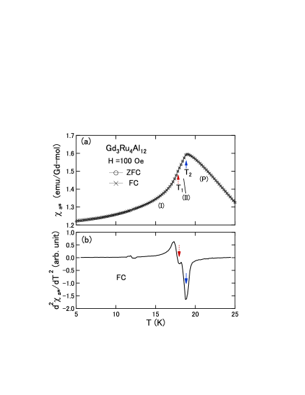
Figure 3: (Color online) (a) Temperature dependence of magnetic susceptibility $\chi_{a*}$. The open circles and crosses denote $\chi$ measured in ZFC (5$\rightarrow$25 K) and FC (25$\rightarrow$5 K) processes under a field of 100 Oe. The broken red and solid blue upward arrows indicate phase transition temperatures. The strength of the fields contains several Oe errors. (b) The second derivative of $\chi_{a*}$ (FC) in relation with temperature. The broken red and solid blue downward arrows correspond to inflection points in $\chi_{a*}$.

Selected temperature dependence of the magnetic susceptibility $M/B$ and specific heat at several fields is presented in Fig. 4, where $T_{1}$ and $T_{2}$ are commonly indicated by the red dotted lines and blue solid lines, respectively. Figure 4 (a) shows $M/B$ under fields directed along the $a$ axis. The measurements were performed with FC processes and we identified the reflection points of $M/B$ as the phase transition points. When fields are applied along the $a$ axis, the IMT phase II only appears in the low field range. Gd₃Ru₄Al₁₂ directly translates from the PM phase into phase I in the high field range.

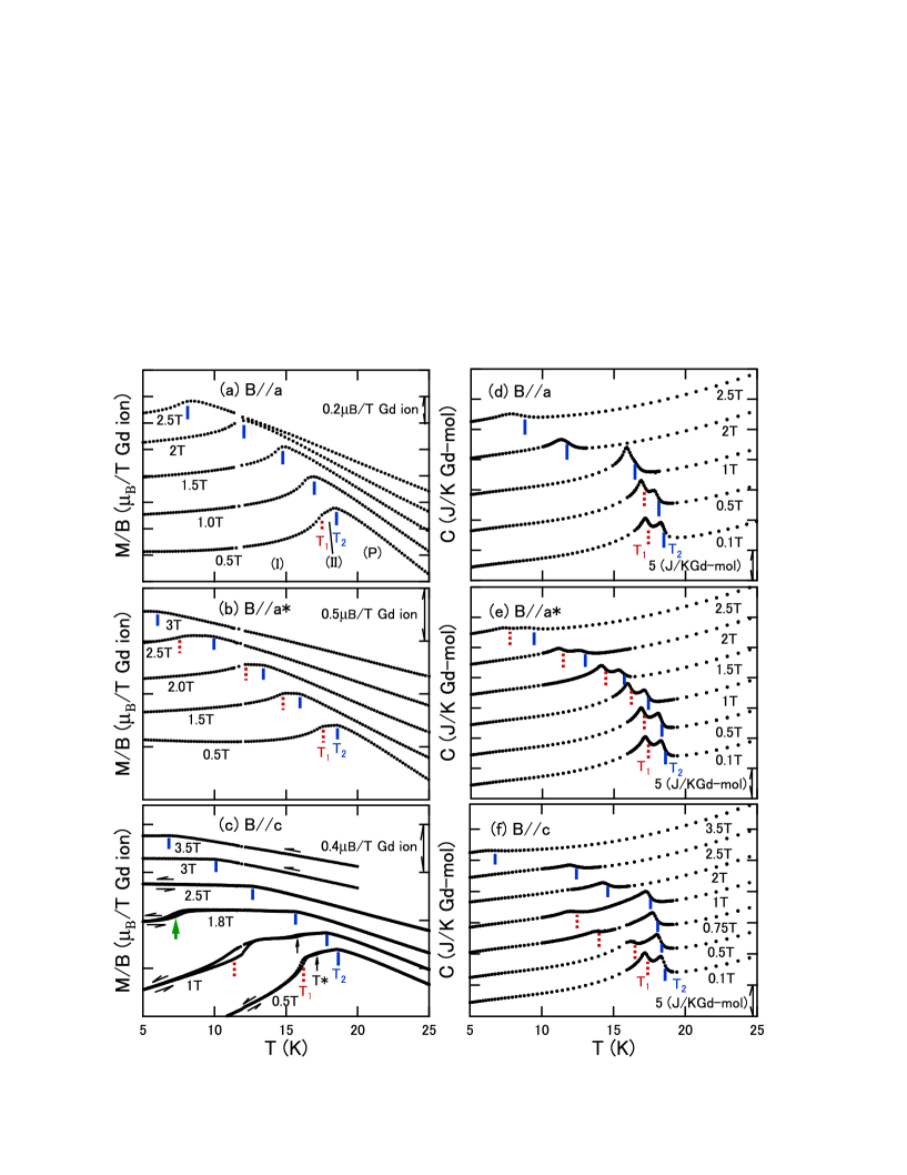
Figure 4: (Color online) Phase transition points of Gd₃Ru₄Al₁₂ observed (a)–(c) in the temperature dependence of magnetization and (d)–(f) in the specific heat. The fields are directed along the (a), (d) $a$ axis; (b), (d) $a^{*}$ axis; (e) and (f) $c$ axis. The red dotted lines and blue solid lines commonly indicate $T_{1}$ and $T_{2}$, respectively. The bold green arrow in panel (c) indicates the phase II/phase III transition point at 1.8 T. The origin of each set of data is shifted for ease of viewing. $T^{*}$ in (c) panel denotes the weak anomalies that may not be phase transition points (see text).

Magnetic susceptibility $M/B$ under several fields directed along the $a^{*}$ axis are presented in Fig. 4 (b). The measurements were performed FC processes. When fields are applied along the $a^{*}$ axis, phase II appears even in the high field range. As evident in Fig. 4 (b), one of the characteristic features of the IMT phase II is the weak temperature dependence in $M/B(T)$. In other words, $M/B$ behaves like a transverse susceptibility in phase II.

In Fig. 4 (c), magnetic susceptibility $M/B$ under fields directed along the $c$ axis are presented. The measurements were performed with FC and field heat (FH) processes in succession at 0.5, 1, 1.8 and 2.5 T, and with FC process at 3 and 3.5 T. When the field is directed along the $c$ axis, $M/B(T)$ shows hysteresis loops at $T_{1}$ in the range $0.3\leq B\leq 2$ T. We identified the inflection points in $M/B$ as $T_{2}$ and centers of the hysteresis loops as $T_{1}$. The bold green upward arrow denotes the phase II/phase III transition points at 1.8 T. We have found an additional phase III in the intermediate fields for ${\bm{B}}\parallel c$. As indicated in Fig. 4 (c) by black upward arrows and symbol $T^{*}$, small anomalies are observed between $T_{1}$ and $T_{2}$ in the field range $0.3\leq B\leq 1.5$ T. However, we could not observe any anomaly in the specific heat at $T^{*}$ as mentioned later. Probably, the anomalies at $T^{*}$ in $M/B$ does not indicate phase transition. As shown in Fig. 4 (c), the IMT phase II appears over the wide temperature ranges in the intermediate field range. Attention should be paid to the temperature dependence of $M/B$ in phase II. When fields are weak, $M/B$ shows some temperature dependence in phase II, but when the field becomes slightly strong, $M/B$ is almost temperature-independent in this phase. Apparently, $M/B$ is a transverse susceptibility in phase II at slightly strong fields. In phase I, $M/B$ shows larger temperature dependence. Apparently, the component of the longitudinal magnetic susceptibility exists in phase I.

The specific heat $C$ at several fields under the fields directed along the $a$ axis are presented in Fig. 4 (d). Corresponding to the successive phase transitions at $T_{1}$ and $T_{2}$, clear $\lambda$-shaped peaks are observed in the specific heat at low fields. In the present study, we identified the phase transition points as the middle points on the right-side slopes of the peaks. The two peaks shown at low fields change into a single peak at high fields. This behavior of the transition points is consistent with that observed in the $M/B$ shown in Fig. 4 (a).

In Fig. 4 (e), specific heat $C$ at several fields under the fields directed along the $a^{*}$ axis are shown. Corresponding to the successive phase transitions at $T_{1}$ and $T_{2}$, clear $\lambda$-shaped peaks are observed as well. The IMT phase II is observed even in high fields similar to the case of observation of the magnetic susceptibility presented in Fig. 4 (b).

Specific heat $C$ at several fields under the fields directed along the $c$ axis are presented in Fig. 4 (f). Clear $\lambda$-shaped peaks are observed at $T_{1}$ and $T_{2}$. The IMT phase II occupies a wide temperature range at intermediate field range. We could not find any indication of phase transition at $T^{*}$ in the specific heat. Probably, the anomalies at $T^{*}$ are so not indicate phase transitions. They may indicate certain domain motion in Phase II.

IV.2 The magnetic phase transitions with changing field

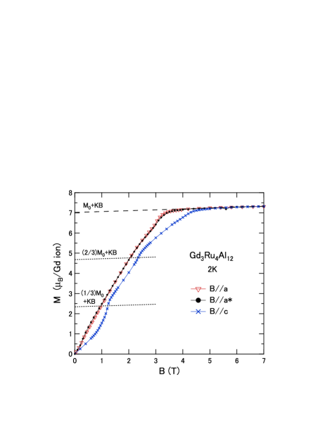
Figure 5: (Color online) Magnetization curves of Gd₃Ru₄Al₁₂ at 2 K in a field increasing process. The fields are directed along the $a$, $a^{*}$ and $c$ axes. The broken line is a fit to the formula $M(B)=M_{0}+KB$ in the range $5.6<B<7$ T for ${\bm{B}}\parallel c$. Here, $M_{0}$ is a constant independent of the field and $K$ is a proportion constant. The doted lines are guides for eye denoting the functions $M(B)=FM_{0}+KB$ $(F=1/3$, 2/3).

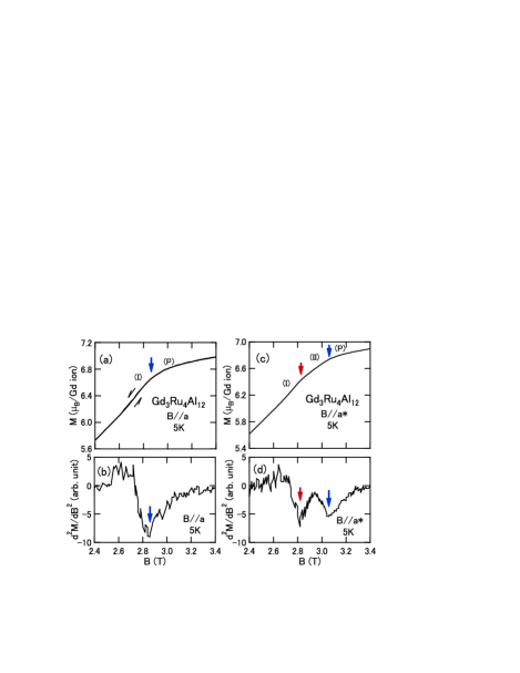
Figure 6: (Color online) (a) Data of $M(B)$ of Gd₃Ru₄Al₁₂ for ${\bm{B}}\parallel a$ at 5 K. (b) The second derivative of $M$ in panel (a) with the elevating field process. (c) Data of $M(B)$ Gd₃Ru₄Al₁₂ for ${\bm{B}}\parallel a*$. (d) The second derivative of $M$ in panel (c). The arrows are indications of phase transition points.

The field dependence of magnetization $M$ of Gd₃Ru₄Al₁₂ at 2 K is displayed in Fig. 5. Overall, the magnetic anisotropy is clearly seen, i.e. $ab$ is an easy plane of magnetization and $c$ is a difficult axis of magnetization. The anisotropy in the $ab$ plane is very small. The additional phase III appears in the intermediate field range $1.25<B<2.4$ T when the field is applied along the $c$ axis at 2 K. Regardless of the difference in field direction, $M$ shows a tendency to increase approximately linearly with magnetic field in the high field range. We assume that $M$ at high fields can be described using $M(B)=M_{0}+KB$. Here, $M_{0}$ is a constant that does not depend on the field and $K$ is a proportion constant. The broken line in Fig. 5 is a fit to the data for ${\bm{B}}\parallel c$ in the range $5.6<B<7$ T. The magnetization $M_{0}=7.02$ $\mu_{\rm B}$ obtained for ${\bm{B}}\parallel c$ agrees with that expected for Gd³⁺ ($S=7/2$). The proportion constant $K$ is estimated to be 4.3$\times 10^{-2}$ $\mu_{\rm B}$T^-1 (2.4$\times 10^{-2}$ emu). If we assume that $K$ arises from Pauli paramagnetism from Ru 4$d$ electrons, it is three orders larger than that for usual transition metals Kriessman1954 . However, this is not the heavy fermion behavior. As we mention later, the low temperature specific heat of Gd₃Ru₄Al₁₂ is not $T$-linear in the very low temperature range. To determine the accurate magnetization processes as field functions, more precise and wide range measurements in the high field range are needed. As shown in Fig. 5, two spin-flopping-like anomalies appear in $M$ for ${\bm{B}}\parallel c$ axis at around 1.25 and 2.4 T. The dotted lines in Fig. 5 are $M$ calculated from the formula $M(B)=FM_{0}+B$ ($F=1/3$, 2/3). Apparently, the spin-flopping-like anomalies appear at the points where the magnetization of Gd ions is approximately equal to $(1/3)M_{0}$ and $(2/3)M_{0}$.

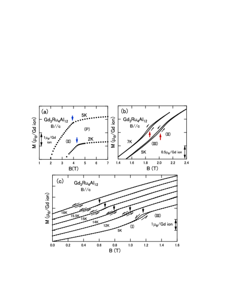
Figure 7: (Color online) Data of $M(B)$ of Gd₃Ru₄Al₁₂ for $B\parallel c$ at several temperatures. (a) $M(B)$ in the high field range, (b) in the intermediate field range, and (c) in the low field range. The arrows indicate the phase transition points.

Figure 6 (a) presents the $M(B)$ curve for ${\bm{B}}\parallel a$ at 5 K. The blue downward arrow indicates the phase I/PM phase transition point at 2.86 T. Here, we regard the reflection point as the phase transition point. Figure 6 (b) shows the second derivative of $M$ in panel (a) with elevating field process. The minimum point in this figure corresponds to the reflection point. When the field is directed along the $a$ axis, Gd₃Ru₄Al₁₂ translates from phase I to PM phase directly.

Fig. 6 (c) shows the $M(B)$ curve for $B\parallel a^{*}$ at 5 K, and Fig. 6 (d) shows the second derivative of $M$ in panel (c). The red arrows at a lower field side and the blue arrows at a higher field side indicate the phase I/phase II transition point at 2.82 T and the phase II/PM phase transition point at 3.06 T. The minimum points shown in the second derivative of $M$ shown in Fig. 6 (d) correspond to these transition points, respectively. When the fields are directed along the $a^{*}$ axis, phase II appears in the intermediate field range even at low temperatures.

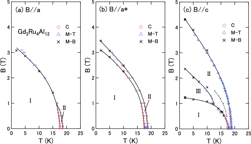
Figure 8: (Color online) Magnetic phase diagrams of Gd₃Ru₄Al₁₂ for (a) ${\bm{B}}\parallel a$, (b) ${\bm{B}}\parallel a^{*}$, and (c) ${\bm{B}}\parallel c$ axes. The red circles, blue triangles, and black crosses indicate the phase transition points determined from specific heat, and $M/B(T)$ and $M/B(B)$ measurements. Data for $C$ at zero field are taken from the reference Nakamura2018 . The dotted line in the right panel corresponds to $T^{*}$ shown in Fig. 4 (c). This line may not be a phase boundary.

Figure 7 displays the magnetization curves under the fields directed along the $c$ axis. The solid downward blue arrows in Fig. 7 (a) indicate the phase II/PM phase transition that occurs at high fields. The magnetization curves in the intermediate field range shows small hysteresis loops, as shown in Fig. 7 (b). The upward red arrows indicate phase III/phase II transitions and the hysteresis loops imply that this transition is of first order. Similar small hysteresis loops are shown in the low field range, as shown in Fig. 7 (c). The black arrows indicate the phase I/phase III transitions. The hysteresis loops imply that this phase transition is of first order as well. The additional phase III is observed in the intermediate field range when fields are directed along the $c$ axis, which is the hard axis of magnetization. This implies that phase III is induced with spin flopping. It is probable that Gd₃Ru₄Al₁₂ undergoes two successive spin flopping, when fields are applied along the $c$ axis.

IV.3 Magnetic phase diagrams

Analyzing the results of measurements of magnetic susceptibility, magnetization, and specific heat, we determined the magnetic phase diagrams of Gd₃Ru₄Al₁₂, as depicted in Fig. 8. The whole view of the magnetic phase diagrams presented in Fig. 8 is unexpectedly anisotropic for Gd compounds. They look different from the phase diagrams of non-frustrated AFM spin systems. The existence of the IMT phase II implies the existence of geometrical frustration. However, there are several features different from the phase diagrams of the typical frustrated AFMTL’s with weak anisotropy and weak interlayer interactions shown in Fig. 2 in terms of the particulars. Let us take a look at the details. Two successive AFM phase transitions have been observed at zero field. This feature is different from that of the phase diagram in Fig. 2 (b). Two double critical points, or Néel points, exist at zero field instead of the single tetracritical point. For $B\parallel a$, the AFM phase I occupies the low-$T$ and low-$B$ regions. Between phase I and the PM phase, phase II occupies a strip region at low fields. At a glance, this strip region appears similar to that shown in Fig. 2 (a). However, the first-phase transition line shown in Fig. 2 (a) is not observed in Fig. 8 (a). In addition, as shown in Fig. 8 (a), phase I directly contacts the PM phase with a boundary in the high field range. On the other hand, there is a high field phase with umbrella spin structure in Fig. 2 (a). For $B\parallel a^{*}$, the boundaries of phase I/phase II and phase II/PM phase display double lines that do not cross and show the difference from non-frustrated AFM spin systems. Probably, these double lines are clear appearance of frustration. When the field is applied along the $c$ axis, as shown in Fig. 8 (c), phase III appears between phase I and phase II in the intermediate field range and phase II relatively occupies a wide region in the diagram. As mentioned before, the magnetization shows hysteresis loops at the phase I/phase III and phase III/phase II transition points, and therefore, both these transitions are of first order. The dotted line in Fig. 8 (c) corresponds to weak anomalies at $T*$ shown in Fig. 4 (c). This line may not be the phase boundary and may correspond to certain domain motion.

The phase diagrams in Fig. 8 appear as if they are a superposition of two independent non-frustrated AFM spin systems with different anisotropies, at a glance. One is the spin system that has easy plane (the $ab$ plane) type and the other is that having easy axis (the $c$ axis) type. The easy plane-type spin system exhibits a simple single-phase boundary and the easy axis-type spin system shows spin flopping when fields are applied along the $c$ axis, as shown in Fig. 8 (c) and Fig. 5. However, as evident from Figs. 8, there is a feature we cannot understand as the superposition of two independent spin systems. Noted that phase I appears as a lower-temperature phase of phase II but phase II does not appear as a lower-temperature phase of phase I. This implies that these phases do not appear independently. Overall, the magnetic phase diagrams of Gd₃Ru₄Al₁₂ indicate the existence of frustration, but present several distinct appearances from those of the typical Heisenberg model with weak anisotropy and weak interlayer interactions on layered AFMTL’s.

V Discussion

V.1 Single trimer magnetic anisotropy

In Gd₃Ru₄Al₁₂, FM trimers ($S_{r}=21/2$) form the AFMTL at low temperatures Nakamura2018 . First, we discuss the single trimer anisotropy. As shown in Fig. 9, the magnetic anisotropy is observed even in the PM phase in the temperature range below 70 K, where ${\bm{S}_{r}}$ are completed Nakamura2018 . This suggests that magnetic anisotropy is induced by the formation of FM trimer. One possible origin of anisotropy is electromagnetic interaction. Figure 10 displays an FM trimer on which three magnetic moments $\bm{m}_{i}$ ($i=1,2,3;m_{i}=7\mu_{\rm B}$) are placed. Here, the subscripts $i=1,2,3$ indicate the number of vertices, and $\mu_{\rm B}=927.400\times 10^{-26}$ JT^-1 is the Bohr magneton. The vector $\bm{r}_{ij}$ denotes the position of vertex $j$ from vertex $i$. The flux density $\bm{B}_{ij}$ at the vertex $j$ induced by $\bm{m}_{i}$ at the vertex $i$ is given by

$${\bm{B}_{ij}}=-\frac{\mu_{0}}{4\pi r^{3}}\left[{\bm{m}_{i}}-\frac{3({\bm{m}_{i}}\cdot{\bm{r}_{ij}}){\bm{r}_{ij}}}{r^{2}}\right].$$

When the FM trimer is formed at low temperatures, all three magnetic moments are written as ${\bm{m}}$. Therefore, the electromagnetic energy of the trimer is

$$E_{em}=\frac{\mu_{0}}{4\pi r^{3}}\biggl{[}3{\bm{m}}^{2}-3\sum_{ij}\frac{({\bm{m}}\cdot{\bm{r}_{ij}})^{2}}{r^{2}}\biggr{]}$$

at a unit of ${\rm J}$ per ${\bm{S}_{r}}$, where the suffix runs over $(ij=12,23,31)$. This energy becomes the lowest when ${\bm{m}}$ is directed in the $ab$ plane. The electromagnetic energy $E_{em}$ gives rise to the easy plane-type anisotropy, and gives isotropy in the $ab$ plane. However, the amplitude of this energy is approximately 2.7 K per ${\bm{S}_{r}}$. This is too small to explain the anisotropy experimentally observed only for that, as mentioned later.

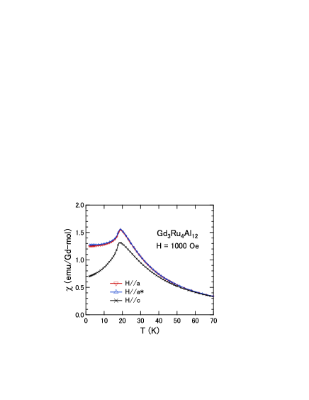
Figure 9: (Color online) Temperature dependence of magnetic susceptibility of Gd₃Ru₄Al₁₂. The applied field is 1000 Oe. The data are taken from the referenceNakamura2018 .

Figure 10: (Color online) Magnetic moments $\bm{m}_{i}$ ($m_{i}=7\mu_{\rm B}$) on an FM trimer. Here, the subscripts $i=1,2,3$ denote the vertices of the triangle. The red spheres indicate Gd ions. The vector $\bm{r}_{ij}$ denotes the position of the vertex $j$ from vertex $i$.

Another possible origin of the single trimer anisotropy is the generation of the orbital angular momentum of Gd³⁺ ($4f^{7},S=7/2$) ions. The 4$f$ electrons of Gd ions do not carry orbital angular momentum in general. However, in the case of Gd₃Ru₄Al₁₂, Gd ions occupy the asymmetric site in the crystal. Therefore, the ions would feel odd parity CEF at each site, which induces the mixing between the $4f$ and $3d$ electrons of the Gd ion, and the Gd ions obtain some angular orbital momentum. This would result in single ion anisotropy. In addition, the existence of orbital moments can lead to spatially anisotropic RKKY interactions Timm2005 , which may induce single trimer anisotropy through a similar mechanism to the case of the above electromagnetic interaction, but detailed mechanism is unknown at present. Probably, a combined effect of the anisotropy due to the odd parity CEF and the electromagnetic interaction is the origin of the single trimer anisotropy.

In any case, we need to determine the magnitude of the single trimer anisotropy in ordered phases experimentally. The magnetic susceptibilities in Fig. 9 at low temperatures are replotted in Fig. 11 on expanded scales. In this figure, magnetic susceptibilities are plotted as the function of $T^{2}$. In phase I, AFM spin waves are expected to contribute to the magnetization at finite temperatures. According to previous theories based on spin wave approximation, the contribution of the three-dimensionally propagating AFM spin waves can be expressed as $M(T)-M(0)\propto T^{2}$ for isotropic systems Kubo1952 ; QTS ; Jaccarino and $M(T)-M(0)\propto T^{1.5}\exp{(-E_{g}/T)}$ for anisotropic systems Jaccarino when the temperatures are sufficiently lower than Néel temperature. Here, $M(0)$ is the magnetization at 0 K and $E_{g}$ is the energy gap in the AFM magnon dispersion,

$$E_{g}=(nk_{\rm B})^{-1}\,\hbar\Omega=(nk_{\rm B})^{-1}\,\hbar\sqrt{\omega_{A}^{2}+2\omega_{ex}\omega_{A}},$$ (3)

at a unit of K per magnon. Here, $n$ is the mole number of propagation medium ${\bm{S}_{r}}$’s, $\Omega$ the lowest precession frequency of magnons, $\hbar\omega_{A}=2\mu_{\rm B}B_{A}$ the crystal magnetic anisotropic energy on single trimer and $\hbar\omega_{ex}=2JSz$ the energy deduced by the exchange interactions from nearest neighbor ${\bm{S}_{r}}$’s of number $z$. The effective anisotropic flux density ${\bm{B}_{A}}$ depends on the directions in general. When the applied external flux density is sufficiently weak, $M$ can be replaced by $\chi$ as

$$\chi(T)-\chi(0) =C_{1}\,T^{2},$$ (4)

$$\chi(T)-\chi(0) =C_{2}\,T^{1.5}\exp{(-E_{g}/T)},$$ (5)

where $C_{1}$ and $C_{2}$ are proportion constants. When $E_{g}$ is large, the dispersion relation is given by,

$$\hbar\omega(k)=\hbar\Omega+D_{a}k^{2},$$ (6)

for small wave number $k$, where $D_{a}$ is proportion constant. The second term in the right side is similar to that for FM magnons. Thus, the numbers of the excited magnons at temperature $T$ is approximately in proportion to $T^{1.5}\exp{(-E_{g}/T)}$.

The solid blue and red curved lines in Fig. 11 are fits to Eq. 5. The calculated data well reproduce the experimentally observed $\chi_{a}$ and $\chi_{a*}$. The temperature dependence of these susceptibilities in the low temperature range can be understood as the contribution from three dimensionally propagate spin waves under ${\bm{B}_{A}}$. The $E_{g}$ obtained are 24 K for $\chi_{a}$ and 29 K for $\chi_{a*}$, being isotropic in the $ab$ plane. On the other hand, it can be seen that $\chi_{c}$ changes as a linear function of $T^{2}$ in the low temperature range. The solid straight line in Fig. 11 is a fit to Eq. 4. The temperature dependence of $\chi_{c}$ is well explained by three dimensionally propagate spin wave contribution without ${\bm{B}_{A}}$ above 4.5 K. It is inferred that single trimer anisotropy of Gd₃Ru₄Al₁₂ is easy plane type. The ${\bm{S}_{r}}$’s which are parallel to the $ab$ plane feels relatively strong ${\bm{B}_{A}}$ along their directions, and the others which are parallel to the $c$ axis only feel weak ${\bm{B}_{A}}$. The observations of ${\bm{B}_{A}}$ indicate that the ${\bm{S}_{r}}$ system of Gd₃Ru₄Al₁₂ is an easy plane type, and the strength of the anisotropy is rather strong. This would have certain degree of characteristics of $XY$ model.

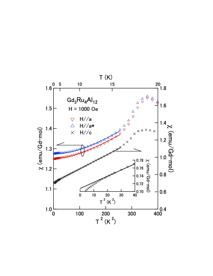
Figure 11: (Color online) Temperature dependence of the magnetic susceptibility of Gd₃Ru₄Al₁₂. The data is taken from Fig. 9 and replotted on a $T^{2}$-scale. The applied field is 1000 Oe. The solid curved lines are fits to Eq. 4 and the solid straight line is a fit to Eq. 5. These lines also indicate the fitting regions. The magnetic susceptibility for ${\bm{H}}\parallel c$ is presented in the inset on expanded scales. The fitting line is expanded to the zero temperature in the inset.

V.2 Spin structure of the ground state

When the anisotropy is weak, the ground state of AFMTL’s are approximately the 120^∘ structure. However, the actual anisotropy is not weak in Gd₃Ru₄Al₁₂. If the single trimer anisotropy is easy plane like, the basal plane of the 120^∘ structure must be parallel to the $ab$ plane. In this case, it is difficult to explain the longitudinal component of magnetic susceptibility in $\chi_{c}$ shown in Fig. 9. In addition, it is difficult to explain the the first order phase transition with spin flopping induced by the flux density ${\bm{B}}\parallel c$ shown in Fig. 8 and Fig. 5. The 120^∘ structure would be change into the umbrella structure in Fig. 2 (a) in the high field region without spin flopping. Probably, we should consider some ground states of Gd₃Ru₄Al₁₂ being different from the 120^∘ structure. Instead of the structure, let us examine the T-shaped structure shown in Fig. 12. In this figure, three ${\bm{S}_{r}}$’s are on the vertexes of the triangle. A pair of ${\bm{S}_{r}}$’s depicted by solid black arrows in opposite directions are directed parallel to the $ab$ plane. The relative directions of these ${\bm{S}_{r}}$’s are fixed in opposite, but the direction of the pair is not strongly fixed in the $ab$ plane. The other ${\bm{S}_{r}}$ illustrated by broken red arrow is directed along the $c$ axis.

Figure 12: (Color online) Spin structures of Gd₃Ru₄Al₁₂ in phase I on the triangle of the trimers. The bold black arrows denote the resultant spin $\bm{S}_{r}$’s ($S_{r}=21/2)$ directed in the $ab$ plane. The broken red arrows indicates the $\bm{S}_{r}$ directed perpendicular to the $c$ axis.

Let us estimate the effective exchange flux densities and anisotropic field from $\chi_{a}$ (${\bm{B}}\parallel a$) and $\chi_{c}$ (${\bm{B}}\parallel c$). A set of T-structured ${\bm{S}_{r}}$’s under the very weak applied flux density ${\bm{B}}_{a}\parallel a$ is depicted in Fig. 13 (a). In this figure, ${\bm{B}_{ex}}$’s indicate the effective flux densities which act on the pair of ${\bm{S}_{r}}$’s. The angle $\phi$ is the angle between the pair and $a$ axis. Figure 13 (b) displays the same T-structure ${\bm{S}_{r}}$’s projected parallel to $a^{*}$ axis. In this figure, ${\bm{B}}_{ex}^{\prime}$ denotes the effective flux density which acts on the ${\bm{S}_{r}}$ depicted by the broken red arrows. Because the in-plane anisotropy is weak, $\phi$ would be equally distributed over the range from $-\pi/2$ to $\pi/2$ due to domain structure. The magnetic susceptibility arising from the pairs become to be a mixture of longitudinal susceptibility and transverse susceptibility when the ${\bm{B}_{a}}$ is applied along the $a$ axis. The $\chi_{a}$ expected is

$$\chi_{a}(0{\rm K}) =2\times\frac{1}{9}N_{\rm A}(2\mu_{\rm B}S_{r})B_{ex}^{-1\,}\frac{1}{\pi}\int_{-\pi/2}^{\pi/2}\sin^{2}\phi\,d\phi$$

$$\quad+\frac{1}{9}N_{\rm A}(2\mu_{\rm B}S_{r})B_{ex}^{\prime-1}$$

in a unit of J/(T² Gd-mol). Here, $N_{\rm A}$ is the Avogadro number. As we mentioned later, the ${\bm{B}}_{ex}$ and ${\bm{B}}_{ex}^{\prime}$ are induced at $T_{2}$ and $T_{1}$, respectively. Since the $T_{1}$ and $T_{2}$ are approximately equal, $B_{ex}$ would be approximately equal to $B_{ex}^{\prime}$. Therefore, we assume $B_{ex}=B_{ex}^{\prime}$. Thus,

$$\chi_{a}(0{\rm K})=\frac{2}{9}N_{\rm A}(2\mu_{\rm B}S_{r})B_{ex}^{-1}.$$ (7)

The $\chi_{a}(1.8{\rm K})$ observed is 1.25 emu/(Gd-mol) as shown in Fig. 11. This is converted into 2.24 $\mu_{\rm B}{\rm T}^{-1}$. Therefore, the effective field $B_{ex}$ is estimated to be 2.08 T. On the other hand, when the field is applied along the $c$ axis, as shown in Fig. 13 (c), the ${\bm{S}_{r}}$ directed along the $c$ axis does not contribute to magnetic susceptibility at 0 K, and only the pair of ${\bm{S}_{r}}$’s directed in the $ab$ plane contribute to the susceptibility, being affected by ${\bm{B}_{A}}$’s. In this case, $\chi_{c}(0{\rm K})$ would be approximately given by,

$$\chi_{c}(0{\rm K})=2\times\frac{1}{9}N(2\mu_{\rm B}S_{r})\left(B_{ex}+B_{A}\right)^{-1}.$$ (8)

The actual $\chi_{c}(1.8{\rm K})$ observed is 0.700 emu/(Gd-mol) as shown in Fig. 11. This is converted into 1.25 $\mu_{\rm B}{\rm T}^{-1}$. Substituting this and $B_{ex}=2.08$ T into Eq. 8, $B_{A}$ is obtained to be 1.64 T. The gain in the anisotropic energy for ${\bm{S}_{r}}$’s which directed in the $ab$ plane is $k_{\rm B}^{-1}(2\mu_{\rm B}S_{r})B_{A}=23.1$ K per ${\bm{S}_{r}}$. This is 8.5 times larger than that estimated from electromagnetic interaction before. If we assume the 120^∘ structure parallel to the $ab$ plane, the ratio $\chi_{a}(0{\rm K})/\chi_{c}(0{\rm K})$ is expected to be 0.89 considering $B_{A}$. This shows significant disagreement with the ratio 1.79 experimentally obtained at 1.8 K.

Assuming the T-structure, we have estimated $B_{ex}$ and $B_{A}$ from the low temperature limits of $\chi$’s. We would be able to calculate $E_{g}$ in Eq. 3 from these. Considering that the number of ${\bm{S}_{r}}$’s is $2/9$ moles, the energy $(nk_{\rm B})^{-1}\hbar\omega_{A}=(nk_{\rm B})^{-1}2\mu_{\rm B}B_{A}$ is obtained to be 9.90 K. If we assume that $B_{ex}$ is determined only by the exchange interactions from the nearest neighbor ${\bm{S}_{r}}$’s, $(nk_{\rm B})^{-1}\hbar\omega_{ex}=(nk_{\rm B})^{-1}(2\times 2\mu_{\rm B}B_{ex})=25.2$ K. Substituting these into Eq. 3, we obtain $E_{g}=24$ K. This agrees with that obtained from the temperature dependence of $\chi$ before.

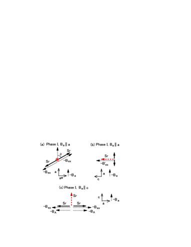
Figure 13: (Color online) The T-structure spins under a weak applied external flux density ${\bm{B}_{a}}\parallel a$, projected parallel to (a) $c$ axis and (b) $a^{*}$ axis. Here, ${\bm{B}_{ex}}$ and ${\bm{B}^{\prime}_{ex}}$ is the internal effective flux density originating from exchange interactions which acts on ${\bm{S}_{r}}$ at each trimer. (c) The T-structure spins projected parallel to $ab$ plane under the ${\bm{B}_{a}}\parallel c$. ${\bm{B}_{A}}$ is the effective anisotropic flux density. The minus signs of the flux densities denote that the magnetic moments and the spins are in opposite direction.

V.3 Spin structure in phase II

If we consider only the interactions among the three ${\bm{S}_{r}}$’s and easy plane anisotropy, the Hamiltonian is written as

$$\mathscr{H}=J\sum_{ij}{\bm{S}_{i}}{\bm{S}_{j}}-D\sum_{i=1,2,3}(S_{i}^{z})^{2},\quad(D<0).$$ (9)

Here, the first summation runs over $ij=12,23,31$. Equation 9 shows that the T-structure has two types of independent operations, which give degeneracies in energy. One is the operations with respect to the 2D rotation of the pair of ${\bm{S}_{r}}$’s indicated by solid black arrows in Fig. 12 around the $c$ axis, and the other is the conversion operation of the directions of the ${\bm{S}_{r}}$ depicted by the broken red arrows with respect to the symmetry plane $ab$. The former type form a 2D rotational group ${\bm{S}_{1}}$, and the latter type forms a cyclic group of order two ${\bm{Z}_{2}}$ with the identity operator. This suggests that these two kinds of degeneracies lead to the successive phase transitions.

We suggest phase II is the phase wherein only ${\bm{S}_{1}}$ symmetry is broken, as shown in Fig. 14. In this figure, a collinear pair of ${\bm{S}_{r}}$’s in the opposite directions is directed in the $ab$ plane and the angle $\phi$ is fixed in the Gd–Al layer. The open circle in Fig. 14 denotes the partial disorder site (trimer). Since the anisotropy in the $ab$ plane is small, the directions of the pair may be distributed in the $ab$ plane by the domain structure at low fields. However, when the fields increase by certain degree, the directions of the pairs would be oriented in the direction perpendicular to the applied field, or in the easy direction to magnetize. Then the pair would show transverse magnetic susceptibility. Actually, as shown in Figs. 4 (b) and (c), the magnetization of Gd₃Ru₄Al₁₂ under the field shows weak temperature dependence in phase II, not being dependent on the directions of applied fields. This is a feature of transverse magnetic susceptibility. When temperature becomes lower than $T_{1}$, ${\bm{Z}_{2}}$ degeneracy is lifted and the spin structure changes into the T-structure. In association with this change, the component of the longitudinal magnetic susceptibility would be added to $\chi_{c}$. Actually, the magnetization at 0.5 and 1 T in Fig. 4 (c) exhibits rapid decrease with decreasing temperature below $T_{1}$. This is considered to be the contribution of longitudinal magnetic susceptibility. As we mentioned before, phase II does not appear at a lower temperature side of phase I, while phase I appears at a lower temperature side of phase II (Fig. 8). This is easily understood if we assume the above partial disorder in phase II.

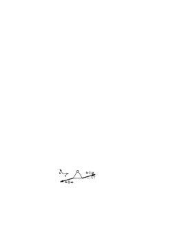
Figure 14: The spin structure in phase II on the triangle of the trimers. A pair of ${\bm{S}_{r}}$’s in opposite directions is directed parallel to the $ab$ plane, and the open circle denotes the partial disordered site (trimer). The angle $\phi$ rotation around the $c$ axis is an element of the ${\bm{S}_{1}}$ group (see text).

So far the spin structure of Gd₃Ru₄Al₁₂ has not been determined by microscopic measurements. However, we discuss a possible orientation to examine the consistency between the ${\bm{S}_{r}}$ structures shown in Figs. 12 and 14 and the successive phase transitions mentioned above. We illustrate the ${\bm{S}_{r}}$ orientation in phase I on a Gd–Al layer in Fig. 15 (a). The small gray triangles indicate trimers. The black arrows denote the ${\bm{S}_{r}}$’s directed in the $ab$ plane, and the red $\odot$ and $\otimes$ indicate ${\bm{S}_{r}}$’s directed along the $c$ axis. As shown in Fig. 15 (a), each triangle of the trimers exhibits a T-structure. Let us note of the ${\bm{S}_{r}}$ surrounded by the broken red circle in Fig. 15 (a). This ${\bm{S}_{r}}$ receives exchange interactions $J$ from six nearest neighbor ${\bm{S}_{r}}$’s in the same layer, but these exchange interactions are canceled out with each other. Such condition would lead to a partial disorder in phase II, as illustrated in Fig. 14. Figure 15 (b) shows the ${\bm{S}_{r}}$’s on two nearest neighbor Gd–Al layers. The broken arrows denote the AFM interlayer exchange integral $J^{\prime}$ which acts between the nearest ${\bm{S}_{r}}$’s on the nearest layers. This interaction generates spontaneous ${\bm{S}_{r}}$’s at the partially disordered sites below $T_{1}$.

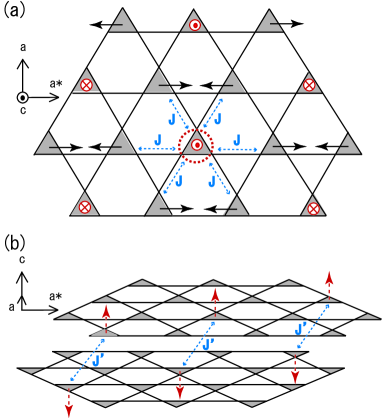
Figure 15: (Color online) A possible ${\bm{S}_{r}}$ structure in phase I. The gray triangles denote the trimers. In this figure, spiral modulations are not considered. (a) The ${\bm{S}_{r}}$’s illustrated by the solid black arrows are directed in the $ab$ plane and those by the red $\odot$ are in the opposite $c$ axis direction and the others by $\otimes$ are in the negative $c$ axis directions. $J$ denotes the exchange integral between nearest ${\bm{S}_{r}}$’s in the same Gd–Al layer. (b) The broken red arrows indicate ${\bm{S}_{r}}$’s directed along the $c$ axis. $J^{\prime}$ denotes the exchange integral between the nearest ${\bm{S}_{r}}$’s on the nearest neighbor Gd–Al layer. In this panel, only a part of the ${\bm{S}_{r}}$’s is illustrated for easy look.

As shown in Fig. 15, the number of ${\bm{S}_{r}}$’s that order at $T_{2}$ is expected to be two times larger than the number of ${\bm{S}_{r}}$’s that order at $T_{1}$. According to the mean field theory of second order phase transitions, the jumps of the magnetic specific heat $\Delta C_{m}$ at $T_{1}$ and at $T_{2}$ are expected to be proportional to the numbers of ${\bm{S}_{r}}$’s, which order at each temperature. We present the magnetic specific heat $C_{m}$ of Gd₃Ru₄Al₁₂ at zero field in the vicinity of phase transition temperatures in Fig. 16. The dotted lines in this figure are fits to lines. The jumps $\Delta C_{m1}$ at $T_{1}$ and $\Delta C_{m2}$ at $T_{2}$ are found to be 2.35 and 4.78 J/(K Gd-mol), respectively, or 0.282$R$ and 0.574$R$ in the unit of gas constant $R$, respectively. The ratio $\Delta C_{m2}/\Delta C_{m1}$ obtained is 2.03, which agrees well with that expected from Fig. 15.

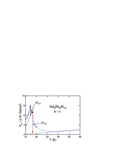
Figure 16: (Color online) Magnetic specific heat jumps of Gd₃Ru₄Al₁₂ at zero field. Data are taken from the reference Nakamura2018 . The dotted lines are fits to lines in the ranges 17.9–18.3 K and 28.2–39.5 K. $\Delta C_{m1}$ and $\Delta C_{m2}$ are obtained as 2.35 and 4.78 J/(K Gd-mol), respectively.

V.4 Spin structure in phase III and the anisotropic energy

As shown in Fig. 8, we have observed the additional phase III in the intermediate field range when fields are directed along the $c$ axis. The hysteresis loops shown in Fig. 7 (c) indicates that the phase I/phase III transition is first order. We present the change in the spin structures assumed in association with this transition in Fig. 17 (c). In this figure, panel (a) denotes the T-structures on A-triangle and B-triangle. These two triangles are on the nearest neighbor layers as shown in Fig. 15 (b). In the absence of the field, the ${\bm{S}_{r}}$’s denoted by the red broken arrows on each triangle are directed along the $c$ axis and canceled out with each other. Between these two ${\bm{S}_{r}}$’s the AFM interaction $J^{\prime}$ is acting (Fig. 15). When the external flux densities ${\bm{B}_{a}}$ are applied along the $c$ axis as illustrated in Fig. 17 (b), the ${\bm{S}_{r}}$’s depicted by the broken red arrows occur to be spin flopping and phase III appears. Figure 17 (c) shows the ${\bm{S}_{r}}$’s in Fig. 17 (b) projected in a direction perpendicular to Fig. 17(b) and parallel to the $ab$ plane. With further increasing the field, the AFM coupling between the broken red arrows in Fig. 17 is broken and the phase III/phase II transition occurs.

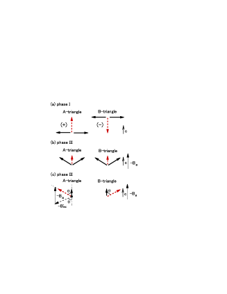
Figure 17: (Color online) (a) The T-structures of ${\bm{S}_{r}}$’s in phase I at zero field. The resultant spins ${\bm{S}_{r}}$’s depicted by the broken red arrows on triangles are directed along the $c$ axis and interact with each other antiferromagnetically. The signs ($+$) and ($-$) correspond to the degrees of freedom of ${\bm{Z}_{2}}$ degeneracy. (b) The canted T-structures in phase III under an applied external flux density ${\bm{B}_{a}}\parallel c$. The broken red arrows indicate the occurrence of spin flopping. The minus sign of ${\bm{B}_{a}}$ denotes the opposite directions of the ${\bm{S}_{r}}$’s and the magnetic moments. (c) The ${\bm{S}_{r}}$’s in panel (b) projected to the direction perpendicular to (b) and parallel to the $ab$ plane.

The spin flopping illustrated in Figs. 17 (a) and (b) occurs at 1.25 T as evident in Fig. 8 (c). We define the angle $\theta$ as shown in Fig. 17 (c), and assume that the anisotropic energy acts on the ${\bm{S}_{r}}$’s depicted by the red broken arrows as $\Delta_{Sr}(1-\cos^{2}{\theta})$ in a unit of J per ${\bm{S}_{r}}$. Figure 18 represents the field dependence of the energy of the pair. When the pair is assumed to be directed in the $c$ axis, the energy of the pair is field independent. On the other hand, when the pair is assumed to be directed in the $ab$ plane at zero field, the magnetization $2\mu_{\rm B}S_{r}(B_{a}/B_{ex}^{\prime})$ is induced by ${\bm{B}_{a}}$. Then the energy of the pair is approximately written as,

$$E(B_{a})=2\Delta_{Sr}-\mu_{\rm B}S_{r}(B_{a}^{2}/B_{ex}^{\prime}),$$

in the weak field range. Since spin flopping occurs at $E=0$, $\Delta_{Sr}$ is given by

$$\Delta_{Sr}=(1/2)\mu_{\rm B}S_{r}(B_{t}^{2}/B_{ex}^{\prime}).$$

Here, the transition field is $B_{t}=1.25$ T and $B^{\prime}_{ex}$($\doteqdot B_{ex}$) is 2.08 T, as we mentioned before. Then, the anisotropic energy $\Delta_{Sr}=3.7\times 10^{-23}$ J per ${\bm{S}_{r}}$, or 2.6 K per ${\bm{S}_{r}}$ is obtained. In phase III, the pair of ${\bm{S}_{r}}$’s depicted by broken red arrows in Fig 17 (b) and (c) are approximately oriented along the high energy directions concerning the anisotropic energy in phase III. Therefore, these ${\bm{S}_{r}}$’s tend to eliminate AFM coupling and change their directions along the $c$ axis in the high field range due to the anisotropic energy. Thus, the phase III/phase II boundary shifts to a lower field side. As evident in Fig. 7 (b), hysteresis loops are observed in magnetization at the phase III/phase II transition points. Therefore, this transition is first order. On the other hand, the anisotropic flux density ${\bm{B}_{A}}$ stabilizes AFM phase II when the applied fields are directed along the $c$ axis, and it would shift the phase II/PM phase boundary to a higher field side. The anisotropic flux density $B_{A}$ is obtained as 1.64 T. This approximately agrees with the shift of phase II/PM phase boundary at 1.8 K as evident in Fig. 8. These are the reasons why phase II occupies the wide region of the phase diagram for ${\bm{B}}\parallel c$. As shown in the inset of Fig. 11, $\chi_{c}$ deviates from the $T^{2}$ behavior below 4.5 K. This deviation may arise from $\Delta_{Sr}$. This energy is sufficiently low compared to $T_{1}$, but it can affect the magnetic susceptibility in the approximate range $T\lesssim 2\Delta_{Sr}$.

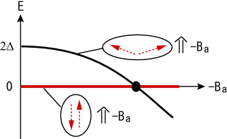
Figure 18: (Color online) (a) Field dependence of the energy of the pair of ${\bm{S}_{r}}$’s. The red bold line denotes the change in the energy when the pair is assumed to be directed along the $c$ axis. The solid black curve indicates the energy when the pair is assumed to be parallel to the $ab$ plane at zero field and canted by the applied flux density.

V.5 Low energy magnetic excitations and long period structures

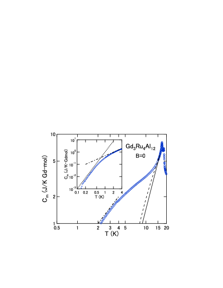
Figure 19: (Color online) Magnetic specific heat $C_{m}$ of Gd₃Ru₄Al₁₂ at zero field on a log$T$-log$C_{m}$ plot. Experimental data (open blue circles) are taken from the reference Nakamura2018 . The solid line is the eye guide, which indicates the slope of $C_{m}\propto T^{3}$. The broken line is the eye guide, which denotes $C_{m}$ with $E_{g}=24$ K (see text). The dotted-broken line is the eye guide, which indicates the slope of $C_{m}\propto T$. The inset shows $C_{m}$ in the low temperature range on a log$T$-log$C_{m}$ plot. The dotted line and dotted-broken line in the inset are eye guides, which indicate the slopes of $C_{m}\propto T^{3}$ and $C_{m}\propto T$, respectively.

The magnetic susceptibility of Gd₃Ru₄Al₁₂ in phase I can be explained by the three-dimensionally propagating spin waves or magnons. On the other hand, the specific heat of Gd₃Ru₄Al₁₂ in phase I shows peculiar behaviors. Figure 19 displays the magnetic specific heat $C_{m}$ of Gd₃Ru₄Al₁₂ at zero field on a log$T$-log$C_{m}$ plot. In this figure, the open blue circles indicate experimental data of $C_{m}$. It is well known that 3D AFM magnons contribute to the specific heat in proportion to $T^{3}$ when the magnon dispersion is gapless QTS . The solid line in Fig. 19 is the temperature dependence of $C_{m}$ expected from AFM magnons without energy gap. When magnon dispersion is written by Eq. 6, $C_{m}$ is given by,

$$C_{m}\propto e^{-(E_{g}/T)}\left[\frac{5}{2}\,T^{\frac{3}{2}}+2E_{g}\,T^{\frac{1}{2}}+\frac{2}{3}(E_{g})^{2}\,T^{-\frac{1}{2}}\right].$$

The broken line in Fig. 19 is $C_{m}$ of AFM magnons with energy gap $E_{g}=24$ K. The exponential factor on the right side mainly determines the temperature dependence. Both calculated data are normalized at 16 K, which is the high temperature end of the fitting range of magnetic susceptibility shown in Fig. 11. As evident in Fig. 19, both contributions from magnons rapidly decrease with decreasing temperature, therefore, we cannot reproduce $C_{m}$ experimentally observed by adding these two at any ratio. The actual $C_{m}$ of Gd₃Ru₄Al₁₂ decreases more slowly with decreasing temperature. This means that certain low energy excitations other than magnons exist in phase I at low temperatures. It is known that a heavy fermion often coexists with AFM magnons Furuno1985 ; Kadowaki1986 . However, the low energy excitation in Gd₃Ru₄Al₁₂ is not a heavy fermion. The inset in Fig. 19 displays $C_{m}$ in the low temperature range on a log$T$-log$C_{m}$ plot. The dotted-broken line and the dotted line are the eye guides which indicate the slopes of the functions $C_{m}\propto T$ and $C_{m}\propto T^{3}$, respectively. The temperature dependence of $C_{m}$ approximately follows $T^{3}$ behavior below 0.5 K, being contradictory to heavy fermion state. In addition to this, no $T^{2}$ behavior is observed in the low temperature electrical resistivity of Gd₃Ru₄Al₁₂ Nakamura2018 . It is probable that certain low energy quasi-particles which do not contribute to magnetization may contribute to the low temperature $C_{m}$ of Gd₃Ru₄Al₁₂. For example, vortexes proposed by Kawamura and Miyashita may be one of the candidates of low energy excitation KawamuraMiyashita1984 .

In the present paper, we have investigated basic properties and spin structures of Gd₃Ru₄Al₁₂ using macroscopic measurements. It is inferred that spiral spin structures may be induced by the competition between far and near neighbors interactions. However, such long period structures and detailed of the low energy excitations should be investigated by microscopic measurements. Unfortunately, Gd ions are good absorbers of neutrons, but investigations by resonant X-ray diffraction may be applicable. For example, the cycloidal magnetic structure of GdRu₂Al₁₀ has been determined by this method Matsumura2017 .

VI Summary

We grew single crystals of Gd₃Ru₄Al₁₂ with the distorted kogome lattice structure wherein stacked AFMTL is formed in association with spin trimerization and the geometrical frustration and interaction-compete-type frustration coexist via the RKKY interaction. Gd₃Ru₄Al₁₂ is found to be a spin system that has a certain degree of strong easy plane-type anisotropy and interlayer interactions. It is highly probable that a partial disorder occurs in this ${\bm{S}_{r}}$’s system. With decreasing temperature, first, the AFM long-range order, wherein ${\bm{S}_{r}}$’s are directed in the $ab$ plane, occurs at $T_{2}$ and IMT phase II appears. This phase is a partial disordered phase wherein 1/3 of ${\bm{S}_{r}}$’s is not arranged and only ${\bm{S}_{1}}$ degeneracy is lifted. With further decreasing temperature, ${\bm{S}_{r}}$’s at the disordered sites exhibit the AFM order wherein a part of them are oriented along the $c$ axis at $T_{1}$. In association with this transition, ${\bm{Z}_{2}}$ degeneracy is lifted. Thus, the noncollinear T-structure of ${\bm{S}_{r}}$ is formed in phase I. We found an additional phase III in intermediate fields directed along the $c$ axis, where spin flopping has occurred in the part of ${\bm{S}_{r}}$’s which is directed in the $c$ axis at zero field. The temperature dependence of the magnetic susceptibilities is well explained by the contribution of three dimensionally propagating magnons. On the other hand, the specific heat in this phase is not understandable only as the contribution of magnons. Certain magnetic excitations other than magnons or heavy fermion may exist owing to the frustration.

References

- (1) J. Niermann and W. Jeitschko, Z. Anorg. Allg. Chem. 628, 2549 (2002).
- (2) Drawing of the crystal structure was produced using VESTA, K. Momma and F. Izumi, J. Appl. Cryst. 44, 1272 (2011).
- (3) W. Ge, H. Ohta, C. Michioka, and K. Yoshimura, J. Phys. (Conf. Scri.) 344, 012023 (2012).
- (4) W. Ge, C. Michioka, H. Ohta, and K. Yoshimura, Soli. Stat. Comm. 195, 1 (2014).
- (5) U3Ru4Al12 is known as a 5 heavy fermion system with non-colinear spin structure., R. Troć, M. Pasturel, O. Tougait, A. P. Sazonov, A. Gukasov, C. Sułkowski, and H. Noël, Phys. Rev. B 85, 064412 (2012).
- (6) D. I. Gorbunov, M. S. Henriques, A. V. Andreev, V. Eigner, A. Gukasov, X. Fabrèges, Y. Skourski, V. Petr̆íc̆ek and J. Wosnitza, Phys. Rev. B 93, 024407 (2016).
- (7) S. Nakamura, S. Toyoshima, N. Kabeya, K. Katoh, T. Nojima, and A. Ochiai, in Proceedings of the International Conference on Strongly Correlated Electrons Systems (SCES2013), Tokyo, JPS Conf. Proc. 3, 014004 (2014).
- (8) S. Nakamura, S. Toyoshima, N. Kabeya, K. Katoh, T. Nojima, and A. Ochiai, Phys. Rev. B 91, 214426 (2015).
- (9) D. I. Gorbunov, M. S. Henriques, A. V. Andreev, A. Gukasov, V. Petříček, N. V. Baranov, Y. Skourski, V. Eigner, M. Paukov, J. Prokleška, and A. P. Gonçalves, Phys. Rev. B 90, 094405 (2014).
- (10) V. Chandragiri, K. K. Iyer, and E. V. Sampathkumaran, Intermetallics 76, 26 (2016).
- (11) V. Chandragiri, K. K. Iyer, and E. V. Sampathkumaran, J. Phys. (Cond. Mat.) 28, 286002 (2016).
- (12) R. B. Griffiths, Phys. Rev. Lett. 23, 17 (1969).
- (13) S. Nakamura, N. Kabeya, M. Kobayashi, K. Araki, K. Katoh, and A. Ochiai, Phys., Rev. B 98, 054410 (2018).
- (14) For review, H. Kawamura, J. Phys. (Cond. Mat.) 10, 4707 (1998).
- (15) S. Miyashita, and H. Kawamura, J. Phys. Soc. Jpn., 54, 3385 (1985).
- (16) S. Miyashita, J. Phys. Soc. Jpn. 55, 3605 (1986).
- (17) P.-É. Melchy, and M. E. Zhitomirsky, Phys. Rev. B 80, 064411 (2009).
- (18) H. Kawamura, A. Caillé, and M. L. Plumer, Phys. Rev. B 41, 4416 (1990).
- (19) R. H. Clark, and W. G. Moulton, Phys. Rev. B 5, 788 (1972).
- (20) M. Poirier, A. Caillé, and M. L. Plumer, Phys. Rev. B 41, 4869 (1990).
- (21) D. Beckmann, J. Wosnitza, and H. v. L’́ohneysen, Phys. Rev. Lett. 71, 2829 (1993).
- (22) H. Kadowaki, K. Ubukoshi, and K. Hirakawa, J. Phys. Soc. Jpn. 56, 751 (1987).
- (23) S. Maegawa, T. Goto, and Y. Ajiro, J. Phys. Soc. Jpn. 57, 1402 (1988).
- (24) B. D. Gaulin, T. E. Mason, and M. F. Collins, J. Z. Larese, Phys. Rev. Lett. 62, 1380 (1989).
- (25) C. J. Kriessman, and Herbert B. Callen, Phys. Rev. 94, 837 (1954).
- (26) C. Timm, and A. H. MacDonald, Phys. Rev. B 71, 155206 (2005).
- (27) R. Kubo, Phys. Rev. 87, 568 (1952).
- (28) C. Kittel in Quantum theory of solids, (John Wiley and Sons Inc., New York, 1964), 2nd printing, Cap. 4, p. 62.
- (29) V. Jaccarino in Magnetism, edited by G. T. Rado and H. Suhl, (Academic Press, New York and London, 1965), Vol. IIA, Cap. 5, p. 319.
- (30) T. Furuno, N. Sato, S. Kunii, T. Kasuya, and W. Sasaki, J. Phys. Soc. Jpn. 54, 1899 (1985).
- (31) Concerning large specific heat coefficients and large -terms of the resistivity in heavy fermion compounds, K. Kadowaki, and S. B. Woods, Solid. Stat. Comm. 58, 507 (1986), K. Miyake, T. Matsuura, and C. M. Varma, Soli. Stat. Comm. 71, 1149 (1989).
- (32) H. Kawamura and S. Miyashita, J. Phys. Soc. Jpn. 53, 4138 (1984). Since the ground state of Gd3Ru4Al12 is not the 120∘ structure, the type of vortexes illustrated in Fig. 2 in this reference may not be excited but the type of vortexes in Fig. 3 may be available.
- (33) T. Matsumura, T. Yamamoto, H. Tanida, and M. Sera, J. Phys. Soc. Jpn. 86, 094709 (2017).