A graphic approach to gauge invariance induced identity

Abstract

All tree-level amplitudes in Einstein-Yang-Mills (EYM) theory and gravity (GR) can be expanded in terms of color ordered Yang-Mills (YM) ones whose coefficients are polynomial functions of Lorentz inner products and are constructed by a graphic rule. Once the gauge invariance condition of any graviton is imposed, the expansion of a tree level EYM or gravity amplitude induces a nontrivial identity between color ordered YM amplitudes. Being different from traditional Kleiss-Kuijf (KK) and Bern-Carrasco-Johansson (BCJ) relations, the gauge invariance induced identity includes polarizations in the coefficients. In this paper, we investigate the relationship between the gauge invariance induced identity and traditional BCJ relations. By proposing a refined graphic rule, we prove that all the gauge invariance induced identities for single trace tree-level EYM amplitudes can be precisely expanded in terms of traditional BCJ relations, without referring any property of polarizations. When further considering the transversality of polarizations and momentum conservation, we prove that the gauge invariance induced identity for tree-level GR (or pure YM) amplitudes can also be expanded in terms of traditional BCJ relations for YM (or bi-scalar) amplitudes. As a byproduct, a graph-based BCJ relation is proposed and proved.

1 Introduction

Gauge invariance has been shown to provide a strong constraint on scattering amplitudes in recent years. It was not only used to solve amplitudes explicitly (see e.g., Boels:2016xhc ; Arkani-Hamed:2016rak ; Boels:2017gyc ; Boels:2018nrr ) but also applied in understanding hidden structures of amplitudes. One interesting application is that a recursive expansion of single-trace Einstein-Yang-Mills (EYM) amplitudes can be determined by gauge invariance conditions of external gravitons in addition with a proper ansatz Fu:2017uzt ; Chiodaroli:2017ngp (the approach based on Cachazo-He-Yuan (CHY) formula Cachazo:2013gna ; Cachazo:2013hca ; Cachazo:2013iea ; Cachazo:2014xea is provided in Teng:2017tbo ). Applying the recursive expansion repeatedly, one expresses an arbitrary tree level single-trace EYM amplitude in terms of pure Yang-Mills (YM) ones whose coefficients are conveniently constructed by a graphic rule Du:2017kpo . This expansion can be regarded as a generalization of the earlier studies on EYM amplitudes with few gravitons Stieberger:2016lng ; Nandan:2016pya ; delaCruz:2016gnm ; Schlotterer:2016cxa . When the relation between gravity amplitudes and single-trace EYM amplitudes are further considered Fu:2017uzt , we immediately expand any tree level gravity amplitude as a combination of Yang-Mills ones. It was shown that the recursive expansion for single-trace EYM amplitudes can be extended to all tree level multi-trace amplitudes via replacing some gravitons by gluon traces appropriately Du:2017gnh .

In the explicit form of the recursive expansion proposed in Fu:2017uzt , gauge invariance conditions for all but one graviton (so-called ‘fiducial graviton’) are naturally encoded into the strength tensors as well as amplitudes with fewer gravitons. Nevertheless, the gauge invariance for the fiducial graviton does not manifest and further implies an nontrivial identity between EYM amplitudes. This identity plays as a consistency condition, which guarantees locality, in the Britto-Cachazo-Feng-Witten (BCFW) recursion approach Britto:2004ap ; Britto:2005fq to the expansion of EYM amplitudes Fu:2017uzt . Equivalently, if we take the gauge invariance condition of the fiducial graviton in the pure YM expansion, we immediately obtain a nontrivial identity for color-ordered YM amplitudes whose coefficients are polynomial functions of Lorentz inner products and depend on both polarizations of gravitons and external momenta. Similar discussions on generating relations for YM amplitudes by imposing gauge invariance can be found in Barreiro:2013dpa ; Boels:2016xhc ; Nandan:2016pya ; Chiodaroli:2017ngp ; Du:2017gnh ; Boels:2017gyc ; Du:2018khm . An application of the gauge invariance induced identity is the proof of the equivalence between distinct approaches Du:2016tbc ; Carrasco:2016ldy ; Du:2017kpo to scattering amplitudes in nonlinear sigma model Du:2018khm .

Apart from the gauge invariance induced identity, color-ordered Yang-Mills amplitudes have also been shown to satisfy Kleiss-Kuijf (KK) Kleiss:1988ne and Bern-Carrasco-Johansson (BCJ) relations Bern:2008qj , which reduce the number of independent amplitudes to $(n-3)!$ (proofs can be found in Stieberger:2009hq ; BjerrumBohr:2009rd ; Feng:2010my ; Chen:2011jxa ). A notable difference from the gauge invariance induced identity is that KK and BCJ relations do not include external polarizations in the coefficients. Thus it seems that the gauge invariance induced identity provides a new relation beyond KK and BCJ relations. However, direct evaluations of several examples Fu:2017uzt ; Chiodaroli:2017ngp ; Du:2017gnh imply that the gauge invariance induced identity is just a combination of BCJ relations. Due to the complexity of the coefficients in the expansion of EYM amplitudes, these examples provided in Fu:2017uzt ; Chiodaroli:2017ngp ; Du:2017gnh cannot be straightforwardly generalized to arbitrary case. Hence there is still lack of a systematical study on the full connection between the gauge invariance induced identity and BCJ relations.

In this paper, we investigate the relationship between an arbitrary gauge invariance induced identity, which is derived from the expansion of tree level single-trace EYM amplitudes or pure GR amplitudes, and general BCJ relations. We propose a ‘refined graphic rule’ in which different types of Lorentz inner products $\epsilon\cdot\epsilon$, $\epsilon\cdot k$ and $k\cdot k$, constructed by half polarizations of gravitons $\epsilon^{\mu}$ and external momenta $k^{\mu}$, are distinguished by different types of lines. Similar graphic rules have already been applied in the study of CHY formula (see Huang:2017ydz ; Lam:2018tgm ). By expressing the coefficients in the gauge invariance induced identity according to the refined graphic rule and collecting those terms with the same structure of the lines corresponding to coefficients $\epsilon\cdot\epsilon$ and $\epsilon\cdot k$ (such a structure is called a skeleton) in particular examples, we find that the gauge invariance induced identity can always be expressed by a combination of BCJ relations.

To generalize our observations to arbitrary case, more hidden structures of graphs should be revealed. We show that a skeleton of a graph corresponding to the gauge invariance induced identity always consists of no less than two maximally connected subgraphs (components) which are mutually disjoint with each other. Any physical graph, which agrees with the refined graphic rule, can be reconstructed by (i) first connecting these components (via $k\cdot k$ lines) into a graph with only two disjoint (called final upper and lower) blocks properly, (ii) then connecting the two disjoint blocks by a $k\cdot k$ line. For any given configuration of the final upper and lower blocks, spurious graphs are also introduced for convenience. We prove that the spurious graphs belonging to different configurations of the two disjoint blocks always cancel in pairs. Hence the sum over all physical graphs containing a same skeleton can be given by summing over both physical and spurious graphs with the same skeleton. A critical observation is that the total contribution of all physical and spurious graphs containing a same configuration of the final upper and lower blocks induces a graph-based BCJ relation which can be expanded in terms of traditional BCJ relations. As a consequence, the general gauge invariance induced identity from the expansion of tree level single-trace EYM amplitude is precisely expanded in terms of (traditional) BCJ relations. Similar discussions are applied to the gauge invariance induced identity of tree level GR amplitudes. The only notable difference is that the transversality of polarizations and momentum conservation in the pure gravity case should be taken into account. By the help of the language of CHY formulas Cachazo:2013gna ; Cachazo:2013hca ; Cachazo:2013iea ; Cachazo:2014xea , we further conclude that the gauge invariance induced identities of Yang-Mills-scalar (YMS) and pure YM amplitudes are combinations of BCJ relations for bi-scalar amplitudes.

The structure of this paper is following. In section 2, we review the expansion of tree level single-trace EYM amplitudes, the gauge invariance induced identity as well as traditional BCJ relations, which will be useful in the remaining sections. The refined graphic rule for the gauge invariance induced identity, which is derived from single-trace EYM amplitudes, as well as the main idea of this paper are provided in section 3. In section 4, direct evaluations of examples are presented. The construction rules of all physical and spurious graphs containing a same skeleton are given in section 5. We show that the total contribution of physical and spurious graphs corresponding to a same configuration of the two disjoint blocks induces the graph-based-BCJ relation which is further proven to be a combination of traditional BCJ relations in section 6. Discussions on identities induced by the gauge invariance of pure GR and YM amplitudes are displayed in section 7. We summarize this work in section 8. Conventions and complicated graphs are included in the appendix.

2 Expansion of tree level single-trace EYM amplitudes, gauge invariance induced identity and traditional BCJ relation

In this section, we review the recursive expansion of single-trace EYM amplitudes, the graphic rule, the gauge invariance induced identity from single-trace EYM amplitudes as well as the BCJ relations for Yang-Mills amplitudes.

2.1 Recursive expansion of tree level single-trace EYM amplitudes

Tree level single-trace EYM amplitude $A(1,2,\dots,r\|\,\mathsf{H})$ with $r$ gluons $1$, $2$, … , $r$ and $s$ gravitons $h_{1}$, $h_{2}$, …, $h_{s}$ can be recursively expanded as (see Fu:2017uzt )

$$A(1,2,\dots,r\|\,\mathsf{H}) = \sum\limits_{\boldsymbol{h}|\,\widetilde{\mathsf{h}}}\,\sum\limits_{\boldsymbol{\sigma}\in\{2,\dots,r-1\}\shuffle\{\boldsymbol{h},h_{a}\}}C_{h_{a}}(\boldsymbol{h})A\bigl{(}1,\boldsymbol{\sigma},r\big{\|}\,\widetilde{\mathsf{h}}\bigr{)},$$ (2.1)

where the full graviton set $\{h_{1},\dots,h_{s}\}$ is denoted by $\mathsf{H}$ and an arbitrarily chosen $h_{a}\in\mathsf{H}$ is called fiducial graviton. The first summation on the RHS is taken over all possible splittings of the set $\mathsf{H}\setminus{h_{a}}\to\boldsymbol{h}|\,\widetilde{\mathsf{h}}$ and all permutations of elements in $\boldsymbol{h}$ for a given splitting. For a fixed splitting $\mathsf{H}\setminus{h_{a}}\to\boldsymbol{h}|\,\widetilde{\mathsf{h}}$ and a fixed permutation of elements in $\boldsymbol{h}$, the second summation is taken over all the possible shuffle permutations $\boldsymbol{\sigma}\in\{2,\dots,r-1\}\shuffle\{\boldsymbol{h},h_{a}\}$ (i.e. permutations in which the relative orders of elements in each set are kept). The coefficient $C_{h_{a}}(\boldsymbol{h})$ for a given splitting $\mathsf{H}\setminus{h_{a}}\to\boldsymbol{h}|\,\widetilde{\mathsf{h}}$, a given permutation $\{i_{1},i_{2},\dots,i_{j}\}$ of elements in $\boldsymbol{h}$ and a given shuffle permutation $\boldsymbol{\sigma}$ is defined by

$$C_{h_{a}}(\boldsymbol{h})\equiv\epsilon_{h_{a}}\cdot F_{i_{j}}\cdot\dots\cdot F_{i_{2}}\cdot F_{i_{1}}\cdot Y_{i_{1}}(\boldsymbol{\sigma}),$$ (2.2)

where the strength tensor $F_{i}^{\mu\nu}$ is

$$F_{i}^{\mu\nu}\equiv k_{i}^{\mu}\epsilon_{i}^{\nu}-k_{i}^{\nu}\epsilon_{i}^{\mu}~{}$$ (2.3)

and $Y_{i_{1}}(\boldsymbol{\sigma})$ denotes the sum of all momenta of gluons $l\in\{1,2,\dots,r-1\}$ s.t. $\boldsymbol{\sigma}^{-1}(l)<\boldsymbol{\sigma}^{-1}(i_{1})$.

2.2 Graphic rule for the pure YM expansion of tree level single-trace EYM amplitudes

Applying the recursive expansion (2.1) repeatedly, we finally express the single-trace EYM amplitude $A(1,2,\dots,r\|\,\mathsf{H})$ in terms of pure YM ones

$$A(1,2,\dots,r\|{\mathsf{H}}) = \sum\limits_{\boldsymbol{\sigma}\in\{2,\dots,r-1\}\shuffle\,\text{perms}\,{\mathsf{H}}}\mathcal{C}(1,\boldsymbol{\sigma},r)A(1,\boldsymbol{\sigma},r).$$ (2.4)

In the above equation, we summed over all possible permutations $\boldsymbol{\sigma}\in\{2,\dots,r-1\}\shuffle\,\text{perms}\,{\mathsf{H}}$ in which the relative order of elements in $\{2,\dots,r-1\}$ is preserved and $\text{perms}\,{\mathsf{H}}$ are all possible permutations of elements in $\mathsf{H}$. The coefficient $\mathcal{C}(1,\boldsymbol{\sigma},r)$ for any permutation $\boldsymbol{\sigma}$ is given by

$$\mathcal{C}(1,\boldsymbol{\sigma},r)=\sum\limits_{\mathcal{F}\in\mathcal{G}(1,\boldsymbol{\sigma},r)}\mathcal{C}^{[\mathcal{F}]},$$ (2.5)

where $\{\mathcal{G}(1,\boldsymbol{\sigma},r)\}$ is used to denote the set of graphs $\mathcal{F}$ constructed by the following graphic rule:

• Define a reference order $\boldsymbol{\rho}$ of gravitons, then all $s$ gravitons are arranged into an ordered set

  $$\mathsf{R}=\{h_{\rho(1)},h_{\rho(2)},\dots,h_{\rho(s)}\}.~{}~{}$$ (2.6)

  The position $\rho^{-1}(l)$ of $l$ ($l\in\mathsf{H}$) in the ordered set $\mathsf{R}$ is called the weight of $l$. Apparently, $h_{\rho(s)}$ is the highest-weight node in $\mathsf{R}$.

• Pick the highest-weight element $h_{\rho(s)}$ (the fiducial graviton for the first step recursive expansion) from the ordered set $\mathsf{R}$, an arbitrary gluon (root) $l\in\{1,2,\dots,r-1\}$ as well as gravitons $i_{1},{i_{2}},\dots,i_{j}\in\mathsf{H}$ s.t. $\sigma^{-1}(l)<\sigma^{-1}(i_{1})<\sigma^{-1}(i_{2})<\dots\sigma^{-1}(i_{j})<\sigma^{-1}(h_{\rho(s)})$. Here the position of $i$ in the permutation $\sigma$ is denoted by $\sigma^{-1}(i)$. By considering each particle in the set $\{l,i_{1},i_{2},\dots,i_{j},h_{\rho(s)}\}$ as a node, we construct a chain $\mathbb{CH}=\left[h_{\rho(s)},i_{j},\dots,i_{1},l\right]$ which starts from the node $h_{\rho(s)}$ towards the node $l$. The graviton $h_{\rho(s)}$, the gluon $l$ and gravitons $i_{1}$, $i_{2}$, … , $i_{j}$ are correspondingly mentioned as the starting node, the ending node and the internal nodes of this chain. We defined the weight of a chain by the weight of the starting node of the chain. The factor associated to this chain is

  $$\epsilon_{h_{\rho(s)}}\cdot F_{i_{j}}\cdot F_{i_{j-1}}\cdot\dots\cdot F_{{i_{1}}}\cdot k_{l}.$$ (2.7)

  Redefine $\mathsf{R}$ by removing ${i_{1}}$, ${i_{2}}$, …, ${i_{j}}$, $h_{\rho(s)}$: $\mathsf{R}\to\mathsf{R}\,^{\prime}=\mathsf{R}\setminus\{{i_{1}},{i_{2}},...,{i_{j}},h_{\rho(s)}\}$.

• Picking $l^{\prime}\in\{1,2,\dots,r-1\}\cup\{{i_{1}},{i_{2}},...,{i_{j}},h_{\rho(s)}\}$, the highest-weight element $h_{\rho^{\prime}(s^{\prime})}$ (which is the fiducial graviton for the second step recursive expansion) in $\mathsf{R}\,^{\prime}$ as well as gravitons ${i^{\prime}_{1}}$, ${i^{\prime}_{2}}$, …, ${i^{\prime}_{j^{\prime}}}\in\mathsf{R}\,^{\prime}$ s.t. $\sigma^{-1}(l^{\prime})<\sigma^{-1}({i_{1}^{\prime}})<\sigma^{-1}({i_{2}^{\prime}})<\dots<\sigma^{-1}({i_{j^{\prime}}^{\prime}})<\sigma^{-1}(h_{\rho^{\prime}(s^{\prime})})$, we define a chain $\mathbb{CH}=\{h_{\rho^{\prime}(s^{\prime})},i^{\prime}_{j^{\prime}},i^{\prime}_{j^{\prime}-1},\dots,i^{\prime}_{1},l^{\prime}\}$ starting from $h_{\rho(s^{\prime})}$ and ending at $l^{\prime}$. This chain is associated with a factor

  $$\epsilon_{h_{\rho^{\prime}(s^{\prime})}}\cdot F_{{i^{\prime}_{j^{\prime}}}}\cdot F_{{i^{\prime}_{j^{\prime}-1}}}\cdot\dots\cdot F_{{i_{1}^{\prime}}}\cdot k_{l^{\prime}}.$$ (2.8)

  Remove ${i_{1}^{\prime}}$,${i_{2}^{\prime}}$, …, ${i_{j^{\prime}}^{\prime}}$, $h_{\rho^{\prime}(s^{\prime})}$ from the ordered set $\mathsf{R}\,^{\prime}$ and redefine $\mathsf{R}\to\mathsf{R}\,^{\prime\prime}=\mathsf{R}^{\prime}\setminus\{{i_{1}^{\prime}},{i_{2}^{\prime}},\dots,{i_{j^{\prime}}^{\prime}},h_{\rho^{\prime}(s^{\prime})}\}$.

• Repeating the above steps until the ordered set $\mathsf{R}$ is empty, we obtain a graph $\mathcal{F}$ in which graviton trees are planted at gluons (roots) $\{1,\dots,r-1\}$. For any given graph $\mathcal{F}$, the product of the factors accompanied to all chains produces a term $\mathcal{C}^{[\mathcal{F}]}$ in the coefficient $\mathcal{C}(1,\boldsymbol{\sigma},r)$ in eq. (2.4). Thus the final expression of $\mathcal{C}(1,\boldsymbol{\sigma},r)$ is given by summing over all possible graphs constructed by the above steps, i.e. eq. (2.5).

2.3 Gauge invariance induced identity from tree level single-trace EYM amplitudes

Gauge invariance requires that an EYM amplitude has to vanish when the ‘half’ graviton polarization $\epsilon_{h_{i}}$ is replaced by momenta $k_{h_{i}}$ for any $h_{i}\in\mathsf{H}$. Consequently, the pure-YM expansion eq. (2.4) should become zero under the replacement $\epsilon_{h_{i}}\to k_{h_{i}}$. Assuming that the half polarization $\epsilon_{h_{i}}$ is included in the coefficients in eq. (2.4), our discussion can be classified into the following two cases:

• If $h_{i}$ is the highest-weight element $h_{\rho(s)}$ (the fiducial graviton for the first-step expansion) in the reference order $\mathsf{R}$, it must be a starting node of some chain but cannot be an internal node of any chain. The gauge invariance condition for $h_{i}$ is not manifest and implies the following nontrivial relation for pure Yang-Mills amplitudes

  $$\sum\limits_{\boldsymbol{\sigma}\in\{2,\dots,r-1\}\shuffle\,\text{perms}\,{\mathsf{H}}}\mathcal{C}(1,\boldsymbol{\sigma},r)\big{|}_{\scriptsize\epsilon_{h_{\rho(s)}}\to k_{h_{\rho(s)}}}A(1,\boldsymbol{\sigma},r)=0,$$ (2.9)

  in which the coefficient $\mathcal{C}(1,\boldsymbol{\sigma},r)\big{|}_{\scriptsize\epsilon_{h_{\rho(s)}}\to k_{h_{\rho(s)}}}$ is obtained from eq. (2.5) via replacing $\epsilon_{h_{\rho(s)}}$ by $k_{h_{\rho(s)}}$. In other words, the chains led by $h_{\rho(s)}$ are of the form $k_{h_{\rho(s)}}\cdot F_{i_{j}}\cdot\dots\cdot F_{i_{2}}\cdot F_{i_{1}}\cdot k_{l}$.

• If $h_{i}$ is some graviton other than $h_{\rho(s)}$, it can be either an internal node or a starting node of some chain. The former case vanishes naturally because of the antisymmetry of the strength tensor $F^{\mu\nu}_{h_{i}}$. The latter case is achieved if the gauge invariance condition eq. (2.9) is already satisfied by amplitudes with fewer gravitons because in this case: (i) $h_{i}$ plays as the fiducial graviton for some intermediate-step recursive expansion in the graphic rule, and (ii) the sum over all the graphs, which contain the same chain structure produced by the preceding steps, is proportional to the LHS of the gauge invariance condition (2.9) (with $h_{\rho(s)}\to h_{i}$) for fewer-graviton EYM amplitudes (Elements on chains produced by the preceding steps are considered as gluons).

Since the gauge invariance condition for $h_{i}\neq h_{\rho(s)}$ is always achieved when the identity eq. (2.9) for fewer gravitons holds, our discussion can just be focused on the case with $h_{i}=h_{\rho(s)}$.

2.4 BCJ relation

Tree level color-ordered YM amplitudes have been proven to satisfy the following general BCJ relation (this general BCJ relation was introduced in BjerrumBohr:2009rd ; Chen:2011jxa ):

$$\sum\limits_{\boldsymbol{\sigma}\in\boldsymbol{\beta}\,\shuffle\,\boldsymbol{\alpha}}\,\sum\limits_{l\in\boldsymbol{\beta}}\left(k_{l}\cdot X_{l}(\boldsymbol{\sigma})\right)A(1,\boldsymbol{\sigma},r)=0,$$ (2.10)

where $\boldsymbol{\beta}$ and $\boldsymbol{\alpha}$ are two ordered sets of external gluons, $X_{l}(\boldsymbol{\sigma})$ denotes the sum of all momenta of gluons $a\in\{1,\boldsymbol{\sigma}\}\cup\boldsymbol{\beta}$ satisfying $\sigma^{-1}(a)<\sigma^{-1}(l)$ (the gluon $1$ is always considered as the first one in the permutation $\boldsymbol{\sigma}$). In this paper, we the expression on the LHS of the eq. (2.10) is denoted as

$$\mathcal{B}(1\,|\,\boldsymbol{\beta},\boldsymbol{\alpha}\,|\,r)=\sum\limits_{\boldsymbol{\sigma}\in\boldsymbol{\beta}\,\shuffle\,\boldsymbol{\alpha}}\,\sum\limits_{l\in\boldsymbol{\beta}}\left(k_{l}\cdot X_{l}(\boldsymbol{\sigma})\right)A(1,\boldsymbol{\sigma},r).$$ (2.11)

3 Refined graphic rule and the main idea

In the previous section, we have shown that the gauge invariance condition for a single-trace EYM amplitude induces a nontrivial identity eq. (2.9) for pure Yang-Mills ones. The difference from BCJ relation is that coefficients in eq. (2.9) contain not only Mandelstam variables $k_{a}\cdot k_{b}$ but also other two types of Lorentz inner products $\epsilon_{a}\cdot\epsilon_{b}$ and $\epsilon_{a}\cdot k_{b}$ which involve half polarizations $\epsilon^{\mu}$. Such feature can be straightforwardly understood when all strength tensors $F_{i}^{\mu\nu}$ on both types of chains $\epsilon_{a}\cdot F_{i_{j}}\cdot\dots\cdot F_{i_{2}}\cdot F_{i_{1}}\cdot k_{l}$ and $k_{\rho(s)}\cdot F_{i_{j}}\cdot\dots\cdot F_{i_{2}}\cdot F_{i_{1}}\cdot k_{l}$ are expanded according to the definition (2.3). As shown by explicit examples in Fu:2017uzt , the identity eq. (2.9) in fact can be expanded in terms of BCJ relations eq. (2.10) without referring any property of external polarizations $\epsilon_{i}^{\mu}$. Nevertheless, this observation cannot be trivially extended to the general identity eq. (2.9) because of the complexity of coefficients in eq. (2.9). Thus the relationship between the gauge invariance induced identity eq. (2.9) and BCJ relation eq. (2.10) is still unclear. In this section, we propose a refined graphic rule and show the main idea for studying the relationship between the identity eq. (2.9) and BCJ relation eq. (2.10), which will be helpful for our generic study in the coming sections.

3.1 Refined graphic rule for single trace tree-level EYM amplitudes

In the graphs constructed by the rule in section 2, the three types of Lorentz inner products $\epsilon_{a}\cdot\epsilon_{b}$, $\epsilon_{a}\cdot k_{b}$ and $k_{a}\cdot k_{b}$ cannot be distinguished. To investigate the general relationship between the gauge invariance induced identity (2.9) and BCJ relation eq. (2.10), we propose the following graphic rule by expanding all strength tensors $F_{a}^{\mu\nu}$ s.t. the three types of Lorentz inner products are represented by three distinct types of lines:

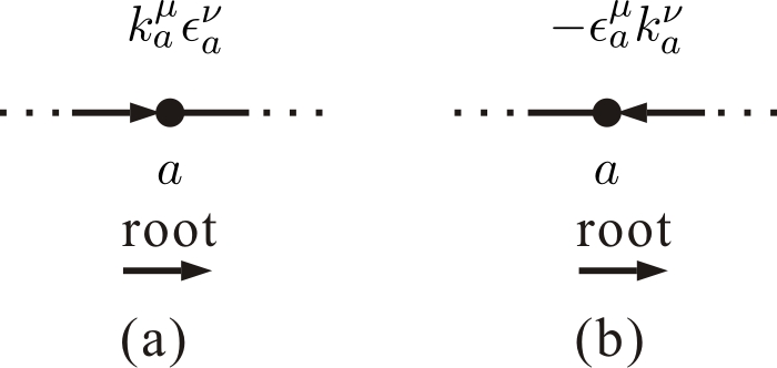
Figure 1: Two types of internal nodes of chains

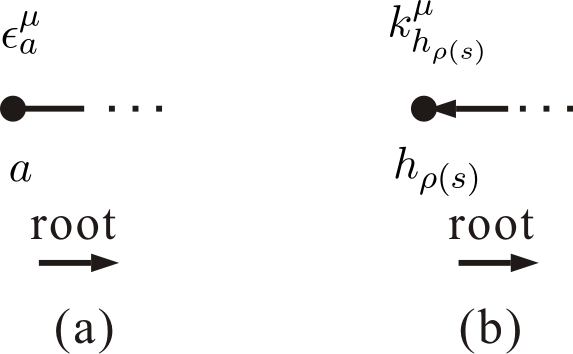
Figure 2: Two types of starting points of chains.

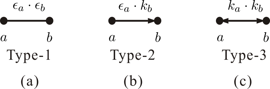
Figure 3: Three types of lines between nodes.

• Internal nodes In the original graphic rule, each internal node stands for a strength tensor $F_{a}^{\mu\nu}$. When $F_{a}^{\mu\nu}$ is expanded into $k_{a}^{\mu}\epsilon_{a}^{\nu}-k_{a}^{\nu}\epsilon_{a}^{\mu}$, the corresponding internal node represents either $k_{a}^{\mu}\epsilon_{a}^{\nu}$ or $-k_{a}^{\nu}\epsilon_{a}^{\mu}$. Here the momentum $k_{a}^{\mu}$ and the ‘half’ polarization $\epsilon_{a}^{\nu}$ are respectively presented by an ingoing arrow line and an outcoming solid line. Then the strength tensor $F_{a}^{\mu\nu}$ becomes the sum of the two graphs in Fig. 1. As shown in Fig. 1 (a), we associate a plus with an arrow pointing to the direction of root. An arrow pointing deviate from root is associated with a minus (see Fig. 1 (b)).

• Starting nodes of chains In the gauge invariance induced identity (2.9), each starting node of a chain is associated with either a ‘half’ polarization $\epsilon_{a}^{\mu}$ of some element other than $h_{\rho(s)}$ or the momentum $k_{h_{\rho(s)}}^{\mu}$ of the highest-weight element $h_{\rho(s)}$ in the ordered set $\mathsf{R}$. Thus two distinct types of starting nodes are required. Noting that all chains are directed to roots, we introduce these two types of starting nodes Fig. 2 (a) and (b) by removing $(...\cdot k)$ and $(-1)(...\cdot\epsilon)$ from the internal nodes shown by Fig. 1 (a) and (b) respectively.

• Ending nodes of chains Each internal/starting node of a chain or a root (the element in the original gluon set $\{1,\dots,r\}$) can also be the ending node of another chain. The contraction of an ending node $b$ of some chain with its neighbor on the same chain always has the form $(...\cdot k_{b})$. Therefore, the ending node of a chain should be attached by a line of form $k_{a}\cdot k_{b}$ or $\epsilon_{a}\cdot k_{b}$.

• Three types of lines between nodes Contractions of Lorentz indices are represented by connecting lines associated to nodes together. There are three distinct types of lines as shown by figure 3 (a) (type-1), (b) (type-2) and (c) (type-3) corresponding to the Lorentz inner products $\epsilon_{a}\cdot\epsilon_{b}$, $\epsilon_{a}\cdot k_{b}$ and $k_{a}\cdot k_{b}$.

With the above improvement, the coefficients $\mathcal{C}(1,\boldsymbol{\sigma},r)\Big{|}_{\epsilon_{h_{\rho(s)}}\to k_{h_{\rho(s)}}}$ of the gauge invariance induced identity eq. (2.9) is then written by summing over all refined graphs. Thus eq. (2.9) becomes

$$\sum\limits_{\boldsymbol{\sigma}\in\{2,\dots,r-1\}\shuffle\,\text{perms}\,{\mathsf{H}}}\left[\sum\limits_{\mathcal{F}\in\mathbb{G}(1,\boldsymbol{\sigma},r)}\mathcal{D}^{[\mathcal{F}]}\right]\,A(1,\boldsymbol{\sigma},r)=0,$$ (3.1)

where $\mathbb{G}(1,\boldsymbol{\sigma},r)$ denotes the set of all refined graphs which are allowed by the permutation $\{1,\boldsymbol{\sigma},r\}$ according to the refined graphic rule. It is worth noting that a given graph $\mathcal{F}$ can be allowed by various permutations.

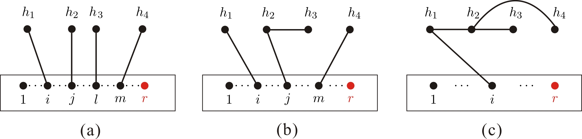
Figure 4: Examples of old-version graphs for the gauge invariance induced identity eq. (2.9). Here, the node $h_{4}$ denotes $k^{\mu}_{h_{4}}$, while the nodes $h_{1}$, $h_{2}$ and $h_{3}$ denote $\epsilon^{\mu}_{h_{1}}$, $\epsilon^{\mu}_{h_{2}}$ and $\epsilon^{\mu}_{h_{3}}$, respectively. We color the element $r$ by red to remind that the element $r$ always plays as the rightmost element in any permutation corresponding to a given graph. Only $1,\dots,r-1$ can be roots.

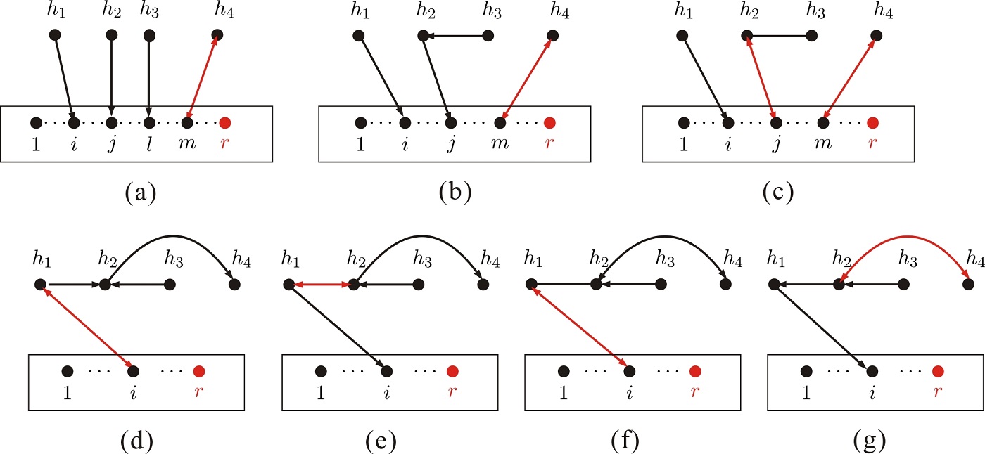
Figure 5: Graphs constructed by the refined graphic rule. The graph (a) corresponds to the old-version graph Fig. 4 (a), the graphs (b) and (c) correspond to the old-version graph Fig. 4 (b), while the graphs (d)-(g) correspond to the old-version graph Fig. 4 (c).

3.1.1 Examples for the refined graphic rule

Now we take the identity induced by the gauge invariance of the amplitude $A(1,\dots,r\|\,h_{1},h_{2},h_{3},h_{4})$ as an example. We assume the reference order is $\mathsf{R}=\{h_{1},h_{2},h_{3},h_{4}\}$ and consider the gauge invariance induced identity eq. (3.1) with $\epsilon_{h_{4}}\to k_{h_{4}}$.

Example-1  For any given permutation $\boldsymbol{\sigma}\in\{2,\dots,r-1\}\shuffle\{h_{1}\}\shuffle\{h_{2}\}\shuffle\{h_{3}\}\shuffle\{h_{4}\}$, there must be old-version graphs Fig. 4 (a) contributing terms of the form $(k_{h_{4}}\cdot k_{m})(\epsilon_{h_{3}}\cdot k_{l})(\epsilon_{h_{2}}\cdot k_{j})(\epsilon_{h_{1}}\cdot k_{i})$ ($i,j,l,m\in\{1,\dots,r-1\}$) to the coefficient $\mathcal{C}(1,\boldsymbol{\sigma},r)|_{\tiny\epsilon_{h_{\rho(s)}}\to k_{h_{\rho(s)}}}$. The refined graph for such a coefficient is shown by Fig. 5 (a), in which each chain led by $h_{1}$, $h_{2}$ or $h_{3}$ consists of only one type-2 line, while the chain led by $h_{4}$ is a type-3 line.

Example-2  For any permutation $\boldsymbol{\sigma}\in\{2,\dots,r-1\}\shuffle\{h_{4}\}\shuffle\{h_{2},h_{3}\}\shuffle\{h_{1}\}$, there exist old-version graphs Fig. 4 (b) consisting of three chains $(k_{h_{4}}\cdot k_{m})$, $(\epsilon_{h_{3}}\cdot F_{h_{2}}\cdot k_{j})$ and $(\epsilon_{h_{1}}\cdot k_{i})$ $(i,j,m\in\{1,\dots,r-1\})$. For given $i,j,m\in\{1,\dots,r-1\}$, the graph Fig. 4 (b) contributes a term $(k_{h_{4}}\cdot k_{m})(\epsilon_{h_{3}}\cdot F_{h_{2}}\cdot k_{j})(\epsilon_{h_{1}}\cdot k_{i})$ to $\mathcal{C}(1,\boldsymbol{\sigma},r)|_{\tiny\epsilon_{h_{\rho(s)}}\to k_{h_{\rho(s)}}}$. According to the refined graphic rule, this coefficient is given by summing the two graphs Fig. 5 (b) and (c) together:

$$\text{(b)}:(k_{h_{4}}\cdot k_{m})(\epsilon_{h_{3}}\cdot k_{h_{2}})(\epsilon_{h_{2}}\cdot k_{j})(k_{h_{1}}\cdot k_{i}),~{}~{}\text{(c)}:(-1)(k_{h_{4}}\cdot k_{m})(\epsilon_{h_{3}}\cdot\epsilon_{h_{2}})(k_{h_{2}}\cdot k_{j})(k_{h_{1}}\cdot k_{i}).$$ (3.2)

Example-3  For any permutation $\boldsymbol{\sigma}\in\{2,\dots,r-1\}\shuffle\{h_{1},h_{2},\{h_{3}\}\shuffle\{h_{4}\}\}$, there exist old-version graphs Fig. 4 (c) (for $i\in\{1,\dots,r-1\}$) each of which contains two distinct chains $(k_{h_{4}}\cdot F_{h_{2}}\cdot F_{h_{1}}\cdot k_{i})$ and $(\epsilon_{h_{3}}\cdot k_{2})$. Thus the total contribution of such a graph is $(k_{h_{4}}\cdot F_{h_{2}}\cdot F_{h_{1}}\cdot k_{i})(\epsilon_{3}\cdot k_{2})$. According to the refined graphic rule, the coefficient for a given $i\in\{1,\dots,r-1\}$ is provided by the sum of the four graphs Fig. 5 (d), (e), (f) and (g):

$$\text{(d)}:(-1)^{2}(k_{h_{4}}\cdot\epsilon_{h_{2}})(k_{h_{2}}\cdot\epsilon_{h_{1}})(k_{h_{1}}\cdot k_{i})(\epsilon_{h_{3}}\cdot k_{h_{2}})~{}\,\text{(e)}:(-1)(k_{h_{4}}\cdot\epsilon_{h_{2}})(k_{h_{2}}\cdot k_{h_{1}})(\epsilon_{h_{1}}\cdot k_{i})(\epsilon_{h_{3}}\cdot k_{h_{2}})$$

$$\text{(f)}:(-1)(k_{h_{4}}\cdot k_{h_{2}})(\epsilon_{h_{2}}\cdot\epsilon_{h_{1}})(k_{h_{1}}\cdot k_{i})(\epsilon_{h_{3}}\cdot k_{h_{2}})~{}~{}~{}\,\text{(g)}:~{}(k_{h_{4}}\cdot k_{h_{2}})(\epsilon_{h_{2}}\cdot k_{h_{1}})(\epsilon_{h_{1}}\cdot k_{i})(\epsilon_{h_{3}}\cdot k_{h_{2}}).$$ (3.3)

3.2 The main idea

Having established the refined graphic rule, we are now ready for studying the relationship between the gauge invariance induced identity eq. (3.1) and BCJ relation eq. (2.10). In the coming sections, we will prove that the gauge invariance induced identity eq. (3.1) can be expanded into a combination of BCJ relations. The main idea is following:

Step-1 The factorization of coefficients  For any graph $\mathcal{F}$ constructed by the refined graphic rule, the coefficient $\mathcal{D}^{[\mathcal{F}]}$ can be factorized as a product of two coefficients $\mathcal{P}^{[\mathcal{F}^{\prime}]}$ and $\mathcal{K}^{[{\mathcal{F}\setminus\mathcal{F}^{\prime}}]}$ associated with a total factor $(-1)^{\mathcal{N}(\mathcal{F})}$. Here, the skeleton $\mathcal{F}^{\prime}$ is the subgraph which is obtained by deleting all type-3 lines from $\mathcal{F}$. The factor $\mathcal{P}^{[\mathcal{F}^{\prime}]}$ associated to the skeleton $\mathcal{F}^{\prime}$ contains only factors of forms $(\epsilon_{a}\cdot\epsilon_{b})$ and $(\epsilon_{a}\cdot k_{b})$. We use $\mathcal{F}\setminus\mathcal{F}^{\prime}$ to stand for the subgraph which is obtained by deleting all type-1 and 2 lines from $\mathcal{F}$ (i.e. the complement of the skeleton). The factor $\mathcal{K}^{[{\mathcal{F}\setminus\mathcal{F}^{\prime}}]}$ corresponding to ${\mathcal{F}\setminus\mathcal{F}^{\prime}}$ contains only Mandelstam variables $(k_{a}\cdot k_{b})$. The total factor $(-1)^{\mathcal{N}(\mathcal{F})}$ depends on the number $\mathcal{N}(\mathcal{F})$ of arrows pointing deviate from the direction of roots ( except the one connected to the highest-weight node $h_{\rho(s)}$ because we do not associate a minus to the arrow Fig. 2 (b) ). For instance, the factor $\mathcal{D}^{[\mathcal{F}^{\prime}]}$ for the graph Fig. 5 (d) is $(-1)^{2}(\epsilon_{h_{1}}\cdot k_{h_{2}})(\epsilon_{h_{2}}\cdot k_{h_{4}})(\epsilon_{h_{3}}\cdot k_{h_{3}})(k_{h_{1}}\cdot k_{i})$ which can be factorized into $\mathcal{P}^{[\mathcal{F}^{\prime}]}=(\epsilon_{h_{1}}\cdot k_{h_{2}})(\epsilon_{h_{2}}\cdot k_{h_{4}})(\epsilon_{h_{3}}\cdot k_{h_{3}})$ and the factor $\mathcal{K}^{[{\mathcal{F}\setminus\mathcal{F}^{\prime}}]}=(k_{h_{1}}\cdot k_{i})$ with a total sign $(-1)^{\mathcal{N}(\mathcal{F})}=(-1)^{2}$. With this factorization, the LHS of the gauge invariance induced identity eq. (3.1) is expressed by

$$T\equiv\sum\limits_{\boldsymbol{\sigma}\in\{2,\dots,r-1\}\shuffle\,\text{perms}\,{\mathsf{H}}}\biggl{[}\sum\limits_{\mathcal{F}\in\mathbb{G}(1,\boldsymbol{\sigma},r)}(-1)^{\mathcal{N}(\mathcal{F})}\mathcal{P}^{[\mathcal{F}^{\prime}]}\mathcal{K}^{[{\mathcal{F}\setminus\mathcal{F}^{\prime}}]}\biggr{]}\,A(1,\boldsymbol{\sigma},r).$$ (3.4)

Here, we emphasize that a given skeleton $\mathcal{F}^{\prime}$ can belong to different permutations $\boldsymbol{\sigma}\in\{2,\dots,r-1\}\shuffle\,\text{perms}\,{\mathsf{H}}$.

Step-2 Collecting all terms corresponding to the graphs $\mathcal{F}\supset\mathcal{F}^{\prime}$ for any given skeleton $\mathcal{F}^{\prime}$ When all graphs containing the same skeleton are collected together, the expression eq. (3.4) becomes

$$T=\sum\limits_{\mathcal{F}^{\prime}}\mathcal{P}^{[\mathcal{F}^{\prime}]}\biggl{[}\sum\limits_{\begin{subarray}{c}\mathcal{F}\text{~{}s.t.}\\ \mathcal{F}\supset\mathcal{F}^{\prime}\end{subarray}}(-1)^{\mathcal{N}(\mathcal{F})}\mathcal{K}^{[{\mathcal{F}\setminus\mathcal{F}^{\prime}}]}\sum\limits_{\boldsymbol{\sigma}^{\mathcal{F}}}\,A(1,\boldsymbol{\sigma}^{\mathcal{F}},r)\biggr{]},$$ (3.5)

where we summed over (i) all possible skeletons $\mathcal{F}^{\prime}$, (ii) all possible graphs $\mathcal{F}$ which are constructed by the refined graphic rule and satisfy $\mathcal{F}\supset\mathcal{F}^{\prime}$ for a given skeleton $\mathcal{F}^{\prime}$, (iii) all permutations $\boldsymbol{\sigma}^{\mathcal{F}}$ for a given $\mathcal{F}$.

Step-3 Finding out the relationship between terms associated with a skeleton and the LHS of BCJ relations For any given skeleton $\mathcal{F}^{\prime}$ in eq. (3.5), we will prove that the expression in the square brackets can be written in terms of the LHS of BCJ relations.

We first present direct evaluations of simple examples in the next section and then prove the general cases in section 5 and section 6.

4 Direct evaluations

In this section, we show that the expression in the square brackets in eq. (3.5) can be expanded in terms of the LHS of BCJ relations by direct evaluation of simple examples.

4.1 The identity with $\mathsf{H}=\{h_{1}\}$

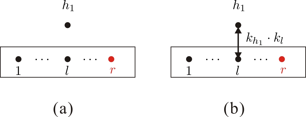
Figure 6: The graph (a) is the skeleton $\mathcal{F}\,^{\prime}$ for the gauge invariance induced identity (3.1) with $\mathsf{H}=\{h_{1}\}$. The graph (b) for $l\in\{1,\dots,r-1\}$ is a typical graph $\mathcal{F}$ containing the skeleton (a).

When the set $\mathsf{H}$ contains only one element $h_{1}$, the LHS of the identity eq. (2.9) has the form

$$T=\sum\limits_{\boldsymbol{\sigma}}(k_{h_{1}}\cdot Y_{h_{1}}(\boldsymbol{\sigma}))A(1,\boldsymbol{\sigma}\in\{2,\dots,r-1\}\shuffle\{h_{1}\},r),$$ (4.1)

which is apparently $\mathcal{B}(1\,|\,\{h_{1}\},\{2,\dots,r-1\}\,|\,r)$ (see eq. (2.11)). Eq. (4.1) can be understood as eq. (3.5) for the specific case $\mathsf{H}=\{h_{1}\}$: (i) The skeleton $\mathcal{F}^{\prime}$ is shown by Fig. 6 (a) and contributes a trivial factor $\mathcal{P}^{[\mathcal{F}^{\prime}]}=1$. (ii) Graphs $\mathcal{F}\supset\mathcal{F}^{\prime}$ (for all $l\in\{1,2,\dots,r-1\}$) are given by Fig. 6 (b) and the kinematic factors $\mathcal{K}^{[\mathcal{F}\setminus\mathcal{F}^{\prime}]}$ are $k_{h_{1}}\cdot k_{l}$. (iii) Permutations allowing the graph Fig. 6 (b) for a given $l\in\{1,2,\dots,r-1\}$ are $\boldsymbol{\sigma}^{l}\in\{2,\dots,l,\{h_{1}\}\shuffle\{l+1,\dots,r-1\}\}$. All together, eq. (3.5) for this example reads

$$T=1\cdot\biggl{[}\sum\limits_{l\in\{1,2,\dots,r-1\}}(k_{h_{1}}\cdot k_{l})\sum\limits_{\boldsymbol{\sigma}^{l}}A(1,\boldsymbol{\sigma}^{l}\in\{2,\dots,l,\{h_{1}\}\shuffle\{l+1,\dots,r-1\}\},r)\biggr{]}.$$ (4.2)

We can collect the coefficients for a given permutation $\boldsymbol{\sigma}\in\{1,\{h_{1}\}\shuffle\{2,\dots,r-1\},r\}$ in the above equation. Noting that each $l$ satisfying $\boldsymbol{\sigma}^{-1}(l)<\boldsymbol{\sigma}^{-1}(h_{1})$ contributes a factor $k_{h_{1}}\cdot k_{l}$, we find that the total factor for $\boldsymbol{\sigma}$ is $(k_{h_{1}}\cdot Y_{h_{1}}(\boldsymbol{\sigma}))$. When all permutations $\boldsymbol{\sigma}\in\{2,\dots,r-1\}\shuffle\{h_{1}\}$ are considered, the expression eq. (4.2) becomes eq. (4.1).

4.2 The identity with $\mathsf{H}=\{h_{1},h_{2}\}$

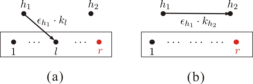
Figure 7: Graphs (a) and (b) are the skeletons $\mathcal{F}^{\prime}$ for the gauge invariance induced identity (3.1) with $\mathsf{H}=\{h_{1},h_{2}\}$.

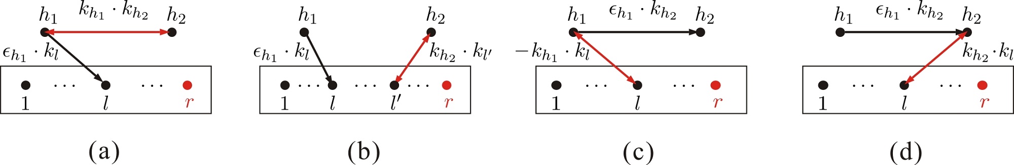
Figure 8: Graphs (a) and (b) are those graphs $\mathcal{F}$ containing the skeleton $\mathcal{F}^{\prime}=\text{Fig.~{}\ref{Fig:Figure2} (a)}$. Graphs containing the skeleton $\mathcal{F}^{\prime}=\text{Fig.~{}\ref{Fig:Figure2} (b)}$ are given by (c) and (d).

The next to simplest example is the identity (2.9) with two gravitons $h_{1}$ and $h_{2}$. Here, we assume that the reference order is $\mathsf{R}=\{h_{1},h_{2}\}$ and consider the gauge invariance condition for $h_{2}$. According to the old-version graphic rule, the LHS of the gauge invariance induced identity eq. (2.9) is written as

$$T = \Bigl{[}k_{h_{2}}\cdot F_{h_{1}}\cdot Y_{h_{1}}+(k_{h_{2}}\cdot Y_{h_{2}})(\epsilon_{h_{1}}\cdot Y_{h_{1}})\Bigr{]}A(1,\{2,\dots,r-1\}\shuffle\{h_{1},h_{2}\},r)$$ (4.3)

$$+ \Bigl{[}(k_{h_{2}}\cdot Y_{h_{2}})(\epsilon_{h_{1}}\cdot Y_{h_{1}})+(k_{h_{2}}\cdot Y_{h_{2}})(\epsilon_{h_{1}}\cdot k_{h_{2}})\Bigr{]}A(1,\{2,\dots,r-1\}\shuffle\{h_{2},h_{1}\},r).$$

When the strength tensor $F^{\mu\nu}$ is expanded, we arrive the following expression

$$T = \Bigl{[}(k_{h_{2}}\cdot k_{h_{1}})(\epsilon_{h_{1}}\cdot Y_{h_{1}})-(k_{h_{2}}\cdot\epsilon_{h_{1}})(k_{h_{1}}\cdot Y_{h_{1}})+(k_{h_{2}}\cdot Y_{h_{2}})(\epsilon_{h_{1}}\cdot Y_{h_{1}})\Bigr{]}A(1,\{2,\dots,r-1\}\shuffle\{h_{1},h_{2}\},r)$$ (4.4)

$$+ \Bigl{[}(k_{h_{2}}\cdot Y_{h_{2}})(\epsilon_{h_{1}}\cdot Y_{h_{1}})+(k_{h_{2}}\cdot Y_{h_{2}})(\epsilon_{h_{1}}\cdot k_{h_{2}})\Bigr{]}A(1,\{2,\dots,r-1\}\shuffle\{h_{2},h_{1}\},r),$$

which can be regarded as a result of the refined graphic rule. In eq. (4.4), only one polarization $\epsilon_{h_{1}}$ appears in the coefficients. Since $\epsilon_{h_{1}}$ can be contracted with the momentum of either $l\in\{1,\dots,r-1\}$ or $h_{2}$, the skeletons $\mathcal{F}^{\prime}$ can be classified into two categories: (i) Fig. 7.(a) (for $l\in\{1,2,\dots,r-1\}$) and (ii) Fig. 7.(b).

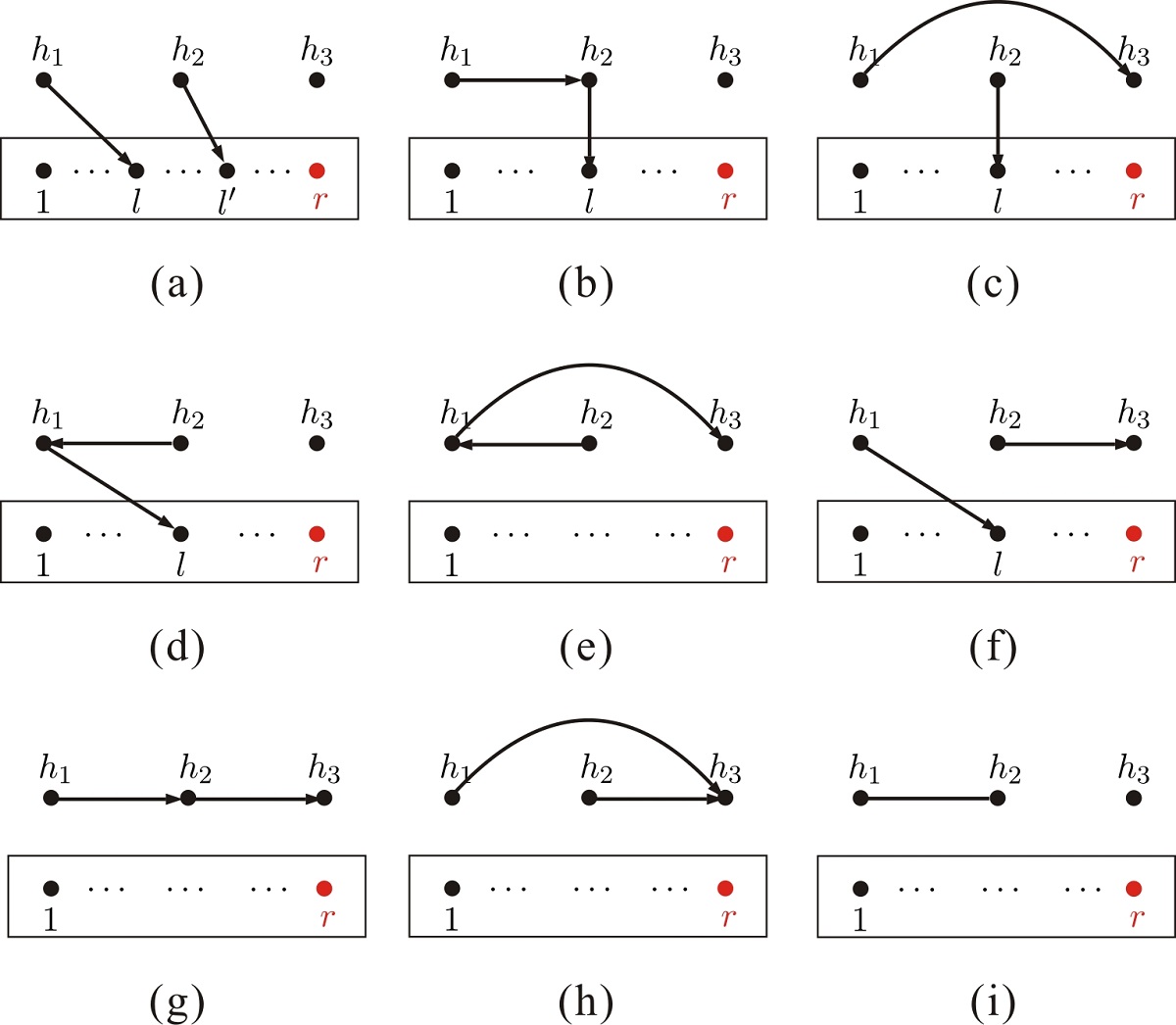
Figure 9: All skeletons for the gauge invariance induced identity with $\mathsf{H}=\{h_{1},h_{2},h_{3}\}$.

The skeleton Fig. 7 (a) with a given $l\in\{1,2,\dots,r-1\}$ contributes a factor $\mathcal{P}^{[\mathcal{F}^{\prime}]}=\epsilon_{h_{1}}\cdot k_{l}$. Graphs $\mathcal{F}$ containing the skeleton Fig. 7 (a) are displayed by Fig. 8 (a) and (b). The factor $\mathcal{K}^{[\mathcal{F}\setminus\mathcal{F}^{\prime}]}$ for $\mathcal{F}=\text{Fig.~{}\ref{Fig:Figure3} (a)}$ is $k_{h_{2}}\cdot k_{h_{1}}$ and the corresponding permutations $\boldsymbol{\sigma}^{\mathcal{F}}$ are

$$\boldsymbol{\sigma}^{\mathcal{F}}\in\{2,\dots,l,\{h_{1},h_{2}\}\shuffle\{l+1,\dots,r-1\}\}.$$ (4.5)

The factor $\mathcal{K}^{[\mathcal{F}\setminus\mathcal{F}^{\prime}]}$ for $\mathcal{F}=\text{Fig.~{}\ref{Fig:Figure3} (b)}$ is $k_{h_{2}}\cdot k_{l^{\prime}}$ $(l^{\prime}=\{1,2,\dots,r-1\})$ and the corresponding permutations $\boldsymbol{\sigma}^{\mathcal{F}}$ satisfy

$$\boldsymbol{\sigma}^{\mathcal{F}}\in\{2,\dots,l,\{h_{1}\}\shuffle\{l+1,\dots,l^{\prime},\{h_{2}\}\shuffle\{l^{\prime}+1,\dots,r-1\}\}\}~{}~{}(1\leq l\leq l^{\prime}\leq r-1)$$

$$\boldsymbol{\sigma}^{\mathcal{F}}\in\{2,\dots,l^{\prime},\{h_{2}\}\shuffle\{l^{\prime}+1,\dots,l,\{h_{1}\}\shuffle\{l+1,\dots,r-1\}\}\}~{}~{}(1\leq l^{\prime}<l\leq r-1).$$ (4.6)

Then the expression in the square brackets of eq. (3.4), which is associated to the skeleton $\mathcal{F}\,^{\prime}=\text{Fig.~{}\ref{Fig:Figure2} (a)}$ for a given $l\in\{1,2,\dots,r-1\}$, is explicitly written as

$$(k_{h_{2}}\cdot k_{h_{1}})\sum\limits_{\boldsymbol{\sigma}}A(1,\boldsymbol{\sigma}\in\{2,\dots,l,\{h_{1},h_{2}\}\shuffle\{l+1,\dots,r-1\}\},r)$$

$$+ \sum\limits_{\begin{subarray}{c}l\,^{\prime}\in\{1,2,\dots,r-1\}\\ \text{s.t.~{}}l\,^{\prime}\geq l\end{subarray}}(k_{h_{2}}\cdot k_{l\,^{\prime}})\sum\limits_{\boldsymbol{\sigma}}A(1,\boldsymbol{\sigma}\in\{2,\dots,l,\{h_{1}\}\shuffle\{l+1,\dots,l^{\prime},\{h_{2}\}\shuffle\{l^{\prime}+1,\dots,r-1\}\}\},r)$$

$$+ \sum\limits_{\begin{subarray}{c}l\,^{\prime}\in\{1,2,\dots,r-1\}\\ \text{s.t.~{}}l\,^{\prime}<l\end{subarray}}(k_{h_{2}}\cdot k_{l\,^{\prime}})\sum\limits_{\boldsymbol{\sigma}}A(1,\boldsymbol{\sigma}\in\{2,\dots,l^{\prime},\{h_{2}\}\shuffle\{l^{\prime}+1,\dots,l,\{h_{1}\}\shuffle\{l+1,\dots,r-1\}\}\},r).$$

The sum over all permutations $\boldsymbol{\sigma}$ in the above expression can be obtained by summing over all possible $\boldsymbol{\sigma}\in\{h_{2}\}\shuffle\boldsymbol{\beta}$ for a fixed $\boldsymbol{\beta}\in\{2,\dots,l,\{h_{1}\}\shuffle\{l+1,\dots,r-1\}\}$ and then summing over all possible $\boldsymbol{\beta}\in\{2,\dots,l,\{h_{1}\}\shuffle\{l+1,\dots,r-1\}\}$. For a fixed $\boldsymbol{\beta}\in\{2,\dots,l,\{h_{1}\}\shuffle\{l+1,\dots,r-1\}\}$, the coefficients for $\boldsymbol{\sigma}\in\{h_{2}\}\shuffle\,\boldsymbol{\beta}$ are collected as

$$\sum\limits_{\begin{subarray}{c}l\,^{\prime}\in\{1,\dots,r-1\}\\ \sigma^{-1}(l\,^{\prime})<\sigma^{-1}(h_{2})\end{subarray}}k_{h_{2}}\cdot k_{l\,^{\prime}} ~{}~{}~{}~{}~{}\text{if }\sigma^{-1}(h_{2})<\sigma^{-1}(l),$$

$$\sum\limits_{\begin{subarray}{c}l\,^{\prime}\in\{1,\dots,r-1\}\\ \sigma^{-1}(l\,^{\prime})<\sigma^{-1}(l)\end{subarray}}k_{h_{2}}\cdot k_{l\,^{\prime}}+\sum\limits_{\begin{subarray}{c}l\,^{\prime}\in\{1,\dots,r-1\}\\ \sigma^{-1}(l)<\sigma^{-1}(l\,^{\prime})<\sigma^{-1}(h_{2})\end{subarray}}k_{h_{2}}\cdot k_{l\,^{\prime}} ~{}~{}~{}~{}~{}\text{if }\sigma^{-1}(l)<\sigma^{-1}(h_{2})<\sigma^{-1}(h_{1}),$$

$$\sum\limits_{\begin{subarray}{c}l\,^{\prime}\in\{1,\dots,r-1\}\\ \sigma^{-1}(l\,^{\prime})<\sigma^{-1}(l)\end{subarray}}k_{h_{2}}\cdot k_{l\,^{\prime}}+\sum\limits_{\begin{subarray}{c}l\,^{\prime}\in\{1,\dots,r-1\}\\ \sigma^{-1}(l)<\sigma^{-1}(l\,^{\prime})<\sigma^{-1}(h_{2})\end{subarray}}k_{h_{2}}\cdot k_{l\,^{\prime}}+k_{h_{2}}\cdot k_{h_{1}} ~{}~{}~{}~{}~{}\text{if }\sigma^{-1}(h_{2})>\sigma^{-1}(h_{1}),$$

where the first line in the above expression comes from the last term of eq. (4.2), the second line gets contributions from both the second and the last terms of eq. (4.2), the third line gets contributions of all the three terms of eq. (4.2). Apparently, all the three cases can be uniformly written as $k_{h_{2}}\cdot X_{h_{2}}(\boldsymbol{\sigma})$ where $X_{h_{2}}(\boldsymbol{\sigma})$ is the sum of all elements (including the element $1$) appearing on the LHS of $h_{2}$ in the permutation $\boldsymbol{\sigma}$. Therefore eq. (4.2) can be reorganized as

$$\sum\limits_{\sigma\in\{h_{2}\}\shuffle\,\boldsymbol{\beta}}\big{(}k_{h_{2}}\cdot X_{h_{2}}(\boldsymbol{\sigma})\big{)}A(1,\boldsymbol{\sigma},r)=\mathcal{B}(1\,|\,\{h_{2}\},\boldsymbol{\beta}\,|\,r),~{}(\text{for }\boldsymbol{\beta}\in\{2,\dots,l,\{h_{1}\}\shuffle\{l+1,\dots,r-1\}\})$$ (4.9)

which is a combination of the LHS of fundamental BCJ relations.

The skeleton $\mathcal{F}^{\prime}=\text{Fig.~{}\ref{Fig:Figure2} (b)}$ contributes a factor $P^{[\mathcal{F}^{\prime}]}=\epsilon_{h_{1}}\cdot k_{h_{2}}$. Graphs $\mathcal{F}\supset\mathcal{F}^{\prime}$ containing the skeleton Fig. 7 (b) are presented by Fig. 8 (c) and (d) which are associated with the factors $\mathcal{K}^{[\mathcal{F}\setminus\mathcal{F}\,^{\prime}]}=-k_{h_{1}}\cdot k_{l}$ and $\mathcal{K}^{[\mathcal{F}\setminus\mathcal{F}\,^{\prime}]}=k_{h_{2}}\cdot k_{l}$, respectively. Permutations $\boldsymbol{\sigma}^{\mathcal{F}}$ corresponding to Fig. 8 (c) and (d) are

$$\boldsymbol{\sigma}^{\mathcal{F}}\in\{2,\dots,l,\{h_{1},h_{2}\}\shuffle\{l+1,\dots,r-1\}\}\text{ and }\boldsymbol{\sigma}^{\mathcal{F}}\in\{2,\dots,l,\{h_{2},h_{1}\}\shuffle\{l+1,\dots,r-1\}\},$$ (4.10)

where $1\leq l\leq r-1$. Thus the expression in the square brackets of eq. (3.4) for the skeleton Fig. 7 (b) is given by

$$- \sum\limits_{l\in\{1,2,\dots,r-1\}}(k_{h_{1}}\cdot k_{l})\sum\limits_{\boldsymbol{\sigma}}A(1,\dots,l,\boldsymbol{\sigma}\in\{h_{1},h_{2}\}\shuffle\{l+1,\dots,r-1\},r)$$ (4.11)

$$+ \sum\limits_{l\in\{1,2,\dots,r-1\}}(k_{h_{2}}\cdot k_{l})\sum\limits_{\boldsymbol{\sigma}}A(1,\dots,l,\boldsymbol{\sigma}\in\{h_{2},h_{1}\}\shuffle\{l+1,\dots,r-1\},r).$$

All possible permutations $\boldsymbol{\sigma}$ in the above expression belong to $\{2,\dots,r-1\}\shuffle\{h_{1}\}\shuffle\{h_{2}\}$, thus one can pick out $\boldsymbol{\sigma}$ and collect all coefficients accompanying with it. The coefficient is $(k_{h_{1}}\cdot Y_{h_{1}}(\boldsymbol{\sigma}))$ for any $\boldsymbol{\sigma}\in\{h_{1},h_{2}\}\shuffle\{2,\dots,r-1\}$ and $(k_{h_{2}}\cdot Y_{h_{2}}(\boldsymbol{\sigma}))$ for any $\boldsymbol{\sigma}\in\{h_{2},h_{1}\}\shuffle\{2,\dots,r-1\}$. Hence Fig. 7 (b) becomes

$$-\sum\limits_{\boldsymbol{\sigma}\in\{h_{1},h_{2}\}\shuffle\{2,\dots,r-1\}}(k_{h_{1}}\cdot Y_{h_{1}}(\boldsymbol{\sigma}))A(1,\boldsymbol{\sigma},r)+\sum\limits_{\boldsymbol{\sigma}\in\{h_{2},h_{1}\}\shuffle\{2,\dots,r-1\}}(k_{h_{2}}\cdot Y_{h_{2}}(\boldsymbol{\sigma}))A(1,\boldsymbol{\sigma},r),$$ (4.12)

which can be further arranged as

$$-\sum\limits_{\boldsymbol{\beta}\in\{h_{2}\}\shuffle\{2,\dots,r-1\}}\,\sum\limits_{\boldsymbol{\sigma}\in\{h_{1}\}\shuffle\,\boldsymbol{\beta}}\,(k_{h_{1}}\cdot X_{h_{1}}(\boldsymbol{\sigma}))\,A(1,\boldsymbol{\sigma},r)$$ (4.13)

$$+\sum\limits_{\boldsymbol{\sigma}\in\{h_{2},h_{1}\}\shuffle\{2,\dots,r-1\}}(k_{h_{2}}\cdot X_{h_{2}}(\boldsymbol{\sigma})+k_{h_{1}}\cdot X_{h_{1}}(\boldsymbol{\sigma}))A(1,\boldsymbol{\sigma},r)$$

$$= -\sum\limits_{\boldsymbol{\beta}\in\{h_{2}\}\shuffle\{2,\dots,r-1\}}\mathcal{B}(1\,|\,\{h_{2}\},\boldsymbol{\beta}\,|\,r)+\mathcal{B}(1\,|\,\{h_{2},h_{1}\},\{2,\dots,r-1\}\,|\,r).$$

Finally, the expression in the square brackets of eq. (3.4) for the skeleton Fig. 7 (b) has been expanded into the LHS of BCJ relations.

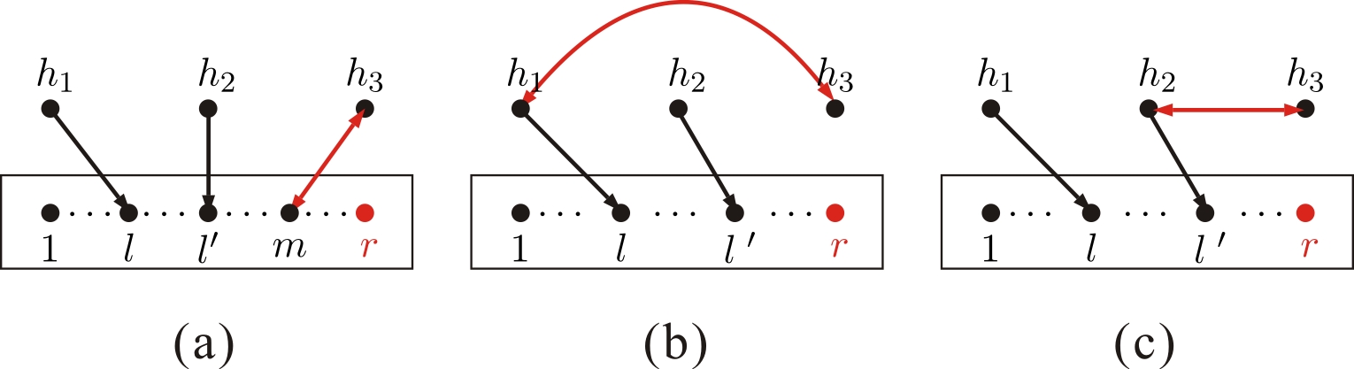
Figure 10: All graphs containing the skeleton $\mathcal{F}\,^{\prime}=\text{Fig.~{}\ref{Fig:Figure4} (a)}$

4.3 The identity with $\mathsf{H}=\{h_{1},h_{2},h_{3}\}$

Relative orders of $h_{1}$, $h_{2}$ and $h_{3}$	Graphs $\mathcal{F}\supset\mathcal{F}^{\prime}$	Sum of coefficients $(-1)^{\mathcal{N}(\mathcal{F})}\mathcal{K}^{[\mathcal{F}\setminus\mathcal{F}^{\prime}]}$
$\{h_{1},h_{2},h_{3}\}$	Fig. 10 (a),(b),(c)	$k_{h_{3}}\cdot Y_{h_{3}}(\boldsymbol{\sigma})+k_{h_{3}}\cdot k_{h_{1}}+k_{h_{3}}\cdot k_{h_{2}}$
$\{h_{1},h_{3},h_{2}\}$	Fig. 10 (a),(b)	$k_{h_{3}}\cdot Y_{h_{3}}(\boldsymbol{\sigma})+k_{h_{3}}\cdot k_{h_{1}}$
$\{h_{3},h_{1},h_{2}\}$	Fig. 10 (a)	$k_{h_{3}}\cdot Y_{h_{3}}(\boldsymbol{\sigma})$
$\{h_{2},h_{1},h_{3}\}$	Fig. 10 (a),(b),(c)	$k_{h_{3}}\cdot Y_{h_{3}}(\boldsymbol{\sigma})+k_{h_{3}}\cdot k_{h_{1}}+k_{h_{3}}\cdot k_{h_{2}}$
$\{h_{2},h_{3},h_{1}\}$	Fig. 10 (a),(c)	$k_{h_{3}}\cdot Y_{h_{3}}(\boldsymbol{\sigma})+k_{h_{3}}\cdot k_{h_{2}}$
$\{h_{3},h_{2},h_{1}\}$	Fig. 10 (a)	$k_{h_{3}}\cdot Y_{h_{3}}(\boldsymbol{\sigma})$

Table 1: Consider the graphs in Fig. 10, which contain the skeleton $\mathcal{F}\,^{\prime}=\text{Fig.~{}\ref{Fig:Figure4} (a)}$. According to the refined graphic rule, the factor $(-1)^{\mathcal{N}(\mathcal{F})}$ for all the three graphs in Fig. 10 is $(-1)^{0}=1$. For fixed $l$, $l^{\prime}$ and a fixed permutation $\boldsymbol{\beta}$ satisfying eq. (4.14), the coefficients $(-1)^{\mathcal{N}(\mathcal{F})}\mathcal{K}^{[\mathcal{F}\setminus\mathcal{F}^{\prime}]}$ for each permutation $\boldsymbol{\sigma}\in\boldsymbol{\beta}\shuffle\{h_{3}\}$ are collected. For example, if the relative order of elements of $\{h_{1},h_{2},h_{3}\}$ in $\boldsymbol{\sigma}\in\boldsymbol{\beta}\shuffle\{h_{3}\}$ is $h_{1}$, $h_{2}$, $h_{3}$, all graphs in Fig. 10 contribute to this permutation. The sum of Fig. 10 (a) for all $m$ satisfying $\boldsymbol{\sigma}^{-1}(m)<\boldsymbol{\sigma}^{-1}(h_{3})$ provides $k_{h_{3}}\cdot Y_{h_{3}}(\boldsymbol{\sigma})$, while graphs Fig. 10 (b) and (c) contribute $k_{h_{3}}\cdot k_{h_{1}}$ and $k_{h_{3}}\cdot k_{h_{2}}$, respectively. Thus the total factor is $k_{h_{3}}\cdot Y_{h_{3}}(\boldsymbol{\sigma})+k_{h_{3}}\cdot k_{h_{1}}+k_{h_{3}}\cdot k_{h_{2}}$, as shown by the first row.

Now we study the gauge invariance induced identity eq. (2.9) with three elements in $\mathsf{H}$. The reference order is chosen as $\mathsf{R}=\{h_{1},h_{2},h_{3}\}$. There are two external polarizations $\epsilon_{h_{1}}$ and $\epsilon_{h_{2}}$ in the coefficients. If both of them are contracted with momenta, we have a factor of the form $\mathcal{P}^{\mathcal{F}^{\prime}}=(\epsilon_{h_{1}}\cdot k_{a})(\epsilon_{h_{2}}\cdot k_{b})$ accompanied to the possible skeletons (a)-(h) in figure 9. Else, if the two polarizations are contracted with each other, the factor $\mathcal{P}^{\mathcal{F}^{\prime}}$ is $\epsilon_{h_{1}}\cdot\epsilon_{h_{2}}$ corresponding to the skeleton $\mathcal{F}^{\prime}=\text{Fig.~{}\ref{Fig:Figure4} (i)}$. Apparently, all skeletons in Fig. 9 are disconnected graphs. For a given skeleton $\mathcal{F}^{\prime}$, we call each maximally connected subgraph a component (the set $\{1,\dots,r\}$ is also considered as a component). According to the number of components and the number of nodes in those components which do not contain $\{1,\dots,r\}$, we classify the skeletons into four categories (1). Fig. 9 (a), (b) and (d), (2). Fig. 9 (c), (f), (3). Fig. 9 (e), (g) and (h), (4). Fig. 9 (i).

(1) All the skeletons Fig. 9 (a), (b) and (d) contain two mutually disjoint components. In each skeleton, one component is the single node $h_{3}$ while the other one is a connected subgraph containing all elements in $\{1,\dots,r\}\cup\{h_{1},h_{2}\}$. We take the skeleton $\mathcal{\mathcal{F}}^{\prime}=\text{Fig.~{}\ref{Fig:Figure4} (a)}$, which is associated with a factor $\mathcal{P}^{[\mathcal{F}\,^{\prime}]}=(\epsilon_{h_{1}}\cdot l)(\epsilon_{h_{2}}\cdot l\,^{\prime})$ (for given $l,l\,^{\prime}\in\{1,2,\dots,r-1\}$), for example. The possible relative orders $\boldsymbol{\beta}$ for elements in $\{1,\dots,r\}\cup\{h_{1},h_{2}\}$ are

$$\boldsymbol{\beta}\in\{2,\dots,l,\{h_{1}\}\shuffle\{l+1,\dots,l^{\prime},\{h_{2}\}\shuffle\{l^{\prime}+1,\dots,r-1\}\}~{}~{}(1\leq l\leq l^{\prime}\leq r-1)$$

$$\boldsymbol{\beta}\in\{2,\dots,l^{\prime},\{h_{2}\}\shuffle\{l^{\prime}+1,\dots,l,\{h_{1}\}\shuffle\{l+1,\dots,r-1\}\}~{}~{}(1\leq l^{\prime}<l\leq r-1).$$ (4.14)

All graphs $\mathcal{F}$ containing the skeleton $\mathcal{F}\,^{\prime}=\text{Fig.~{}\ref{Fig:Figure4} (a)}$ are provided by Fig. 10 (a), (b) and (c). For any fixed $l$, $l^{\prime}$ and a corresponding $\boldsymbol{\beta}$, all possible permutations $\boldsymbol{\sigma}$ corresponding to graphs Fig. 10 (a), (b) and (c) belong to $\boldsymbol{\beta}\shuffle\{h_{3}\}$. We can collect coefficients $(-1)^{\mathcal{N}(\mathcal{F})}\mathcal{K}^{[\mathcal{F}\setminus\mathcal{F}^{\prime}]}$ for each permutation $\boldsymbol{\sigma}\in\boldsymbol{\beta}\shuffle\{h_{3}\}$. As shown by table 1, coefficients for any permutation $\boldsymbol{\sigma}\in\boldsymbol{\beta}\shuffle\{h_{3}\}$ can be uniformly written as $k_{h_{3}}\cdot X_{h_{3}}({\boldsymbol{\sigma}})$. Thus the expression in the square brackets of eq. (3.5) for the skeleton $\mathcal{\mathcal{F}}^{\prime}=\text{Fig.~{}\ref{Fig:Figure4} (a)}$ (with given $l$ and $l^{\prime}$) is expressed by

$$\sum\limits_{\boldsymbol{\beta}}\biggl{[}\sum\limits_{\boldsymbol{\sigma}\in\{h_{3}\}\shuffle\,\boldsymbol{\beta}}(k_{h_{3}}\cdot X_{h_{3}}(\boldsymbol{\sigma}))A(1,\boldsymbol{\sigma},r)\biggr{]}=\sum\limits_{\boldsymbol{\beta}}\mathcal{B}(1\,|\,\{h_{3}\},\boldsymbol{\beta}\,|\,r),$$ (4.15)

where we summed over all $\boldsymbol{\beta}$ satisfy eq. (4.14). Apparently, the expression in the square brackets in the above equation is the LHS of a fundamental BCJ relation.

Figure 11: All graphs $\mathcal{F}$ containing the skeleton $\mathcal{F}^{\prime}=\text{Fig.~{}\ref{Fig:Figure4} (c)}$.

Relative orders of $h_{1}$, $h_{2}$ and $h_{3}$	Graphs $\mathcal{F}\supset\mathcal{F}^{\prime}$	Sum of coefficients $(-1)^{\mathcal{N}(\mathcal{F})}\mathcal{K}^{[\mathcal{F}\setminus\mathcal{F}^{\prime}]}$
$\{h_{1},h_{2},h_{3}\}$	Fig. 11 (a)	$-k_{h_{1}}\cdot Y_{h_{1}}(\boldsymbol{\sigma})$
$\{h_{1},h_{3},h_{2}\}$	Fig. 11 (a)	$-k_{h_{1}}\cdot Y_{h_{1}}(\boldsymbol{\sigma})$
$\{h_{2},h_{1},h_{3}\}$	Fig. 11 (a), (c)	$-(k_{h_{1}}\cdot Y_{h_{1}}(\boldsymbol{\sigma})+k_{h_{1}}\cdot k_{h_{2}})$
$\{h_{2},h_{3},h_{1}\}$	Fig. 11 (b), (d)	$k_{h_{3}}\cdot Y_{h_{3}}(\boldsymbol{\sigma})+k_{h_{3}}\cdot k_{h_{2}}$
$\{h_{3},h_{1},h_{2}\}$	Fig. 11 (b)	$k_{h_{3}}\cdot Y_{h_{3}}(\boldsymbol{\sigma})$
$\{h_{3},h_{2},h_{1}\}$	Fig. 11 (b)	$k_{h_{3}}\cdot Y_{h_{3}}(\boldsymbol{\sigma})$

Table 2: Consider the graphs in Fig. 11, which contain the skeleton $\mathcal{F}\,^{\prime}=\text{Fig.~{}\ref{Fig:Figure4} (c)}$. According to the refined graphic rule, the factor $(-1)^{\mathcal{N}(\mathcal{F})}$ is $-1$ for Fig. 11 (a), (c), $1$ for Fig. 11 (b), (d). For a given $l$ and a given $\boldsymbol{\beta}$ satisfying eq. (4.16), permutations $\boldsymbol{\sigma}$ corresponding to the skeleton $\mathcal{F}^{\prime}=\text{Fig.~{}\ref{Fig:Figure4} (c)}$ belong to $\{h_{1}\}\shuffle\{h_{3}\}\shuffle\boldsymbol{\beta}$ for $\boldsymbol{\beta}$. For any $\boldsymbol{\sigma}\in\{h_{1}\}\shuffle\{h_{3}\}\shuffle\boldsymbol{\beta}$ we collect the coefficients $(-1)^{\mathcal{N}(\mathcal{F})}\mathcal{K}^{[\mathcal{F}\setminus\mathcal{F}^{\prime}]}$ together as we have done in the previous case. Each row shows the expression of the sum of $(-1)^{\mathcal{N}(\mathcal{F})}\mathcal{K}^{[\mathcal{F}\setminus\mathcal{F}^{\prime}]}$ for a given relative order of $h_{1}$, $h_{2}$ and $h_{3}$.

(2) Both skeletons Fig. 9 (c) and (f) contain two mutually disconnected components. In each skeleton, the component which does not contain $\{1,\dots,r\}$ has two nodes with a type-2 line between them. We take the graph Fig. 9 (c) as an example. The factor $\mathcal{P}^{\mathcal{F}^{\prime}}$ for the skeleton Fig. 9 (c) is $(\epsilon_{h_{1}}\cdot k_{h_{3}})(\epsilon_{h_{2}}\cdot k_{l})$. Relative permutations for the elements in the component containing $\{1,\dots,r\}$ are

$$\boldsymbol{\beta}\in\{2,\dots,l,\{h_{2}\}\shuffle\{l+1,\dots,r-1\}\}~{}~{}~{}~{}~{}(1\leq l\leq r-1).$$ (4.16)

All graphs $\mathcal{F}$ satisfying $\mathcal{F}\supset\mathcal{F}\,^{\prime}=\text{Fig.~{}\ref{Fig:Figure4} (c)}$ are presented by Fig. 11 and all possible permutations $\boldsymbol{\sigma}$ allowed by the graphs in Fig. 11 belong to $\boldsymbol{\beta}\shuffle\{h_{1}\}\shuffle\{h_{3}\}$ (for a given $\boldsymbol{\beta}$ in eq. (4.16)). To obtain the expression in the brackets in eq. (3.5) corresponding to the skeleton Fig. 9 (c) for a given $l\in\{1,\dots,r-1\}$, we can collect the coefficients for any given permutation $\boldsymbol{\sigma}\in\boldsymbol{\beta}\shuffle\{h_{1}\}\shuffle\{h_{3}\}$ (see table 2). Then sum over all possible $\boldsymbol{\sigma}\in\boldsymbol{\beta}\shuffle\{h_{1}\}\shuffle\{h_{3}\}$ and all possible $\boldsymbol{\beta}$ satisfying eq. (4.16). From table 2, we find that the coefficients in the first three rows and the last three rows can be respectively written as $-k_{h_{1}}\cdot X_{h_{1}}(\boldsymbol{\sigma})$ and $k_{h_{3}}\cdot X_{h_{3}}(\boldsymbol{\sigma})$. Thus the expression in the square brackets of eq. (3.5) for the skeleton Fig. 9 (c) ($l\in\{1,\dots,r-1\}$) is given by

$$-\sum\limits_{\boldsymbol{\beta}}\biggl{[}\sum\limits_{\boldsymbol{\sigma}\in\{h_{1},h_{3}\}\shuffle\,\boldsymbol{\beta}}(k_{h_{1}}\cdot X_{h_{1}}(\boldsymbol{\sigma}))A(1,\boldsymbol{\sigma},r)\biggr{]} + \sum\limits_{\boldsymbol{\beta}}\biggl{[}\sum\limits_{\boldsymbol{\sigma}\in\{h_{3},h_{1}\}\shuffle\,\boldsymbol{\beta}}(k_{h_{3}}\cdot X_{h_{3}}(\boldsymbol{\sigma}))A(1,\boldsymbol{\sigma},r)\biggr{]},$$ (4.17)

in which the first summation is taken over all $\boldsymbol{\beta}$ satisfying eq. (4.16). The first term in the above expression can be rewritten as

$$- \sum\limits_{\boldsymbol{\beta}}\biggl{[}\sum\limits_{\boldsymbol{\sigma}\in\{h_{1}\}\shuffle\{h_{3}\}\shuffle\,\boldsymbol{\beta}}(k_{h_{1}}\cdot X_{h_{1}}(\boldsymbol{\sigma}))A(1,\boldsymbol{\sigma},r)-\sum\limits_{\boldsymbol{\sigma}\in\{h_{3},h_{1}\}\shuffle\,\boldsymbol{\beta}}(k_{h_{1}}\cdot X_{h_{1}}(\boldsymbol{\sigma}))A(1,\boldsymbol{\sigma},r)\biggr{]}$$ (4.18)

$$= -\sum\limits_{\boldsymbol{\beta}}\sum\limits_{\boldsymbol{\rho}}\mathcal{B}(1\,|\,\{h_{1}\},\boldsymbol{\rho}\in\{h_{3}\}\shuffle\boldsymbol{\beta}\,|\,r)+\sum\limits_{\boldsymbol{\beta}}\biggl{[}\sum\limits_{\boldsymbol{\sigma}\in\{h_{3},h_{1}\}\shuffle\,\boldsymbol{\beta}}(k_{h_{1}}\cdot X_{h_{1}}(\boldsymbol{\sigma}))A(1,\boldsymbol{\sigma},r)\biggr{]}.$$

Since the sum of the last term on the second line of the above equation and the second term of eq. (4.17) is just a combination of LHS of BCJ relations $\sum\limits_{\boldsymbol{\beta}}\mathcal{B}(1\,|\,\{h_{3},h_{1}\},\boldsymbol{\beta}\,|\,r)$, eq. (4.17) is finally arranged as

$$-\sum\limits_{\boldsymbol{\beta}}\sum\limits_{\boldsymbol{\rho}}\mathcal{B}(1\,|\,\{h_{1}\},\boldsymbol{\rho}\in\{h_{3}\}\shuffle\boldsymbol{\beta}\,|\,r)+\sum\limits_{\boldsymbol{\beta}}\mathcal{B}(1\,|\,\{h_{3},h_{1}\},\boldsymbol{\beta}\,|\,r),$$ (4.19)

the first summation in each term is taken over all $\boldsymbol{\beta}$ satisfying eq. (4.16). Thus the expression in the brackets in eq. (3.5) for the skeleton Fig. 9 (c) is written as a combination of the LHS of BCJ relations.

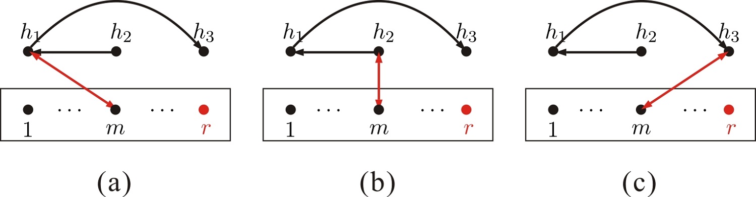
Figure 12: All graphs $\mathcal{F}$ containing the skeleton $\mathcal{F}\,^{\prime}=\text{Fig.~{}\ref{Fig:Figure4} (e)}$.

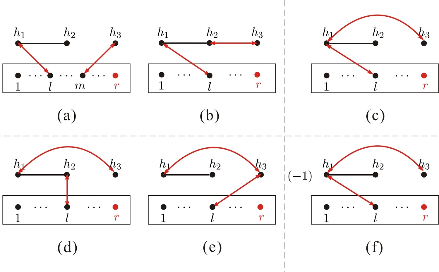
Figure 13: Graphs (a), (b), (d) and (e) are physical graphs, which are constructed by the refined graphic rule, for the skeleton $\mathcal{F}\,^{\prime}=\text{Fig.~{}\ref{Fig:Figure4} (i)}$. Graphs (d) and (e) are spurious graphs for the skeleton $\mathcal{F}\,^{\prime}=\text{Fig.~{}\ref{Fig:Figure4} (i)}$. All spurious graphs cancel with each other.

Relative orders of $h_{1}$, $h_{2}$ and $h_{3}$	Graphs $\mathcal{F}\supset\mathcal{F}\,^{\prime}$	Coefficients $(-1)^{\mathcal{N}(\mathcal{F})}\mathcal{K}^{[\mathcal{F}\setminus\mathcal{F}^{\prime}]}$
$\{h_{1},h_{2},h_{3}\}$	Fig. 12 (a)	$-k_{h_{1}}\cdot Y_{h_{1}}(\boldsymbol{\sigma})$
$\{h_{1},h_{3},h_{2}\}$	Fig. 12 (a)	$-k_{h_{1}}\cdot Y_{h_{1}}(\boldsymbol{\sigma})$
$\{h_{2},h_{1},h_{3}\}$	Fig. 12 (b)	$k_{h_{2}}\cdot Y_{h_{2}}(\boldsymbol{\sigma})$
$\{h_{3},h_{1},h_{2}\}$	Fig. 12 (c)	$k_{h_{3}}\cdot Y_{h_{3}}(\boldsymbol{\sigma})$

Table 3: Total coefficients $(-1)^{\mathcal{N}(\mathcal{F})}\mathcal{K}^{[\mathcal{F}\setminus\mathcal{F}^{\prime}]}$ for permutations allowed by the graphs in Fig. 12.

(3) Each of the skeletons Fig. 9 (e), (g) and (h) consists of two mutually disjoint components. One of them contains all elements of the set $\mathsf{H}=\{h_{1},h_{2},h_{3}\}$ and two type-2 lines between them. The other contains all elements in $\{1,\dots,r\}$. We now study the skeleton $\mathcal{F}\,^{\prime}=\text{Fig.~{}\ref{Fig:Figure4} (e)}$, which gives a factor $\mathcal{P}^{[\mathcal{F}\,^{\prime}]}=(\epsilon_{h_{1}}\cdot k_{h_{3}})(\epsilon_{h_{2}}\cdot k_{h_{1}})$, for instance. All possible graphs satisfying $\mathcal{F}\supset\mathcal{F}\,^{\prime}$ are displayed in Fig. 12. Relative orders of $h_{1}$, $h_{2}$ and $h_{3}$, allowed by the graphs in Fig. 12 are $\{h_{1},\{h_{2}\}\shuffle\{h_{3}\}\}$, $\{h_{2},h_{1},h_{3}\}$ and $\{h_{3},h_{1},h_{2}\}$, whose coefficients $\mathcal{K}^{[\mathcal{F}\setminus\mathcal{F}\,^{\prime}]}$ are collected by table 3. Thus the total contribution from the skeleton reads

$$\sum\limits_{\boldsymbol{\sigma}\in\{2,\dots,r-1\}\shuffle\{h_{1},\{h_{2}\}\shuffle\{h_{3}\}\}}(-k_{h_{1}}\cdot Y_{h_{1}}(\boldsymbol{\sigma}))A(1,\boldsymbol{\sigma},r)$$

$$+ \sum\limits_{\boldsymbol{\sigma}\in\{2,\dots,r-1\}\shuffle\{h_{2},h_{1},h_{3}\}}(k_{h_{2}}\cdot Y_{h_{2}}(\boldsymbol{\sigma}))A(1,\boldsymbol{\sigma},r)+\sum\limits_{\boldsymbol{\sigma}\in\{2,\dots,r-1\}\shuffle\{h_{3},h_{1},h_{2}\}}(k_{h_{3}}\cdot Y_{h_{3}}(\boldsymbol{\sigma}))A(1,\boldsymbol{\sigma},r).$$

When expressing the last two terms respectively by

$$\sum\limits_{\boldsymbol{\beta}\in\{2,\dots,r-1\}\shuffle\{h_{1},h_{3}\}}\mathcal{B}(1\,|\,\{h_{2}\},\boldsymbol{\beta}\,|\,r)-\biggl{[}\sum\limits_{\boldsymbol{\sigma}\in\{2,\dots,r-1\}\shuffle\{h_{1},\{h_{2}\}\shuffle\{h_{3}\}\}}(k_{h_{2}}\cdot X_{h_{2}}(\boldsymbol{\sigma}))A(1,\boldsymbol{\sigma},r)\biggr{]}$$ (4.21)

and

$$\sum\limits_{\boldsymbol{\beta}\in\{2,\dots,r-1\}\shuffle\{h_{1},h_{2}\}}\mathcal{B}(1\,|\,\{h_{3}\},\boldsymbol{\beta}\,|\,r)-\biggl{[}\sum\limits_{\boldsymbol{\sigma}\in\{2,\dots,r-1\}\shuffle\{h_{1},\{h_{2}\}\shuffle\{h_{3}\}\}}(k_{h_{3}}\cdot X_{h_{3}}(\boldsymbol{\sigma}))A(1,\boldsymbol{\sigma},r)\biggr{]},$$ (4.22)

eq. (4.3) becomes

$$\sum\limits_{\boldsymbol{\beta}\in\{2,\dots,r-1\}\shuffle\{h_{1},h_{3}\}}\mathcal{B}(1\,|\,\{h_{2}\},\boldsymbol{\beta}\,|\,r)+\sum\limits_{\boldsymbol{\beta}\in\{2,\dots,r-1\}\shuffle\{h_{1},h_{2}\}}\mathcal{B}(1\,|\,\{h_{3}\},\boldsymbol{\beta}\,|\,r)$$ (4.23)

$$- \sum\limits_{\boldsymbol{\rho}\in\{h_{1},\{h_{2}\}\shuffle\{h_{3}\}\}}\mathcal{B}(1\,|\,\boldsymbol{\rho},\{2,\dots,r-1\}\,|\,r),$$

which is a combination of the LHS of BCJ relations.

Relative orders of $h_{1}$, $h_{2}$ and $h_{3}$	Physical graphs $\mathcal{F}\supset\mathcal{F}\,^{\prime}$	$(-1)^{\mathcal{N}(\mathcal{F})}\mathcal{K}^{[\mathcal{F}\setminus\mathcal{F}^{\prime}]}$ from physical graphs	Spurious graphs $\mathcal{F}\supset\mathcal{F}\,^{\prime}$	Factors from spurious graphs
$\{h_{1},h_{2},h_{3}\}$	Fig. 13 (a),(b)	$-(k_{h_{1}}\cdot k_{l})(k_{h_{3}}\cdot Y_{h_{3}}+k_{h_{3}}\cdot k_{h_{2}})$	Fig. 13 (c)	$-(k_{h_{3}}\cdot k_{h_{1}})(k_{h_{1}}\cdot k_{l})$
$\{h_{1},h_{3},h_{2}\}$	Fig. 13 (a)	$-(k_{h_{1}}\cdot k_{l})(k_{h_{3}}\cdot Y_{h_{3}})$	Fig. 13 (c)	$-(k_{h_{3}}\cdot k_{h_{1}})(k_{h_{1}}\cdot k_{l})$
$\{h_{3},h_{1},h_{2}\}$	Fig. 13 (a)	$-(k_{h_{1}}\cdot k_{l})(k_{h_{3}}\cdot Y_{h_{3}})$	no	0
$\{h_{1},h_{2},h_{3}\}$	no	0	Fig. 13 (f)	$(k_{h_{3}}\cdot k_{h_{1}})(k_{h_{1}}\cdot Y_{h_{1}})$
$\{h_{1},h_{3},h_{2}\}$	no	0	Fig. 13 (f)	$(k_{h_{3}}\cdot k_{h_{1}})(k_{h_{1}}\cdot Y_{h_{1}})$
$\{h_{2},h_{1},h_{3}\}$	Fig. 13 (d)	$-(k_{h_{2}}\cdot Y_{h_{2}})(k_{h_{3}}\cdot k_{h_{1}})$	no	0
$\{h_{3},h_{1},h_{2}\}$	Fig. 13 (e)	$-(k_{h_{1}}\cdot k_{h_{3}})(k_{h_{3}}\cdot Y_{h_{3}})$	no	0

Table 4: For given $l$ and given $\boldsymbol{\beta}$ satisfying eq. (4.24) in the upper part of Fig. 13, relative orders and corresponding factors are collected on the second, third and fourth rows. Relative orders for graphs in the lower part of Fig. 13 and their factors are collected on the last four rows.

(4) The skeleton Fig. 9 (i) is a much more nontrivial example. There are three mutually disjoint components in Fig. 9 (i) which contain the elements $\{1,\dots,r\}$, the single node $h_{3}$ and the subgraph with nodes $h_{1}$ and $h_{2}$, correspondingly. The factor $\mathcal{P}^{[\mathcal{F}\,^{\prime}]}$ for Fig. 9 (i) is $\epsilon_{h_{1}}\cdot\epsilon_{h_{2}}$ and the possible graphs $\mathcal{F}\supset\mathcal{F}\,^{\prime}=\text{Fig.~{}\ref{Fig:Figure4} (i)}$ are shown by Fig. 13 (a), (b), (d) and (e). For a given graph Fig. 13 (a) or (b), in which $h_{1}$ is contracted with an arbitrary $l\in\{1,\dots,r-1\}$, the possible relative orders of elements in $\{h_{1},h_{2}\}\cup\{1,\dots,r-1\}$ satisfy

$$\boldsymbol{\beta}\in\{1,\dots,l,\{h_{1},h_{2}\}\shuffle\{l+1,\dots,r-1\}\}.$$ (4.24)

Hence all permutations contributing to graphs Fig. 13 (a) and (b) have the form $\boldsymbol{\sigma}\in\{h_{3}\}\shuffle\boldsymbol{\beta}$. To get the total contribution of all graphs Fig. 13 (a) and (b), we should collect coefficients $(-1)^{\mathcal{N}(\mathcal{F})}\mathcal{K}^{[\mathcal{F}\setminus\mathcal{F}^{\prime}]}$ together for a given permutation $\boldsymbol{\sigma}\in\{h_{3}\}\shuffle\boldsymbol{\beta}$ (see table 4), then sum over all $\boldsymbol{\beta}$ satisfying eq. (4.24) and all $l\in\{1,\dots,r-1\}$. The total contributions of all graphs Fig. 13 (a) and (b) thus is written as

$$T_{1} = -\sum\limits_{l\in\{1,\dots,r-1\}}(k_{h_{1}}\cdot k_{l})\sum\limits_{\begin{subarray}{c}\small\boldsymbol{\beta}\in\{2,\dots,l,\{h_{1},h_{2}\}\\ \small\shuffle\{l+1,\dots,r-1\}\}\end{subarray}}\biggl{[}\sum\limits_{\small\begin{subarray}{c}{\boldsymbol{\sigma}\in\{h_{3}\}\shuffle\boldsymbol{\beta}}\\ {\boldsymbol{\sigma}^{-1}(h_{2})<\boldsymbol{\sigma}^{-1}(h_{3})}\end{subarray}}(k_{h_{3}}\cdot Y_{h_{3}}(\boldsymbol{\sigma})+k_{h_{3}}\cdot k_{h_{2}})A(1,\boldsymbol{\sigma},r)$$ (4.25)

$$+\sum\limits_{\small\begin{subarray}{c}{\boldsymbol{\sigma}\in\{h_{3}\}\shuffle\boldsymbol{\beta}}\\ {\boldsymbol{\sigma}^{-1}(h_{1})<\boldsymbol{\sigma}^{-1}(h_{3})<\boldsymbol{\sigma}^{-1}(h_{2})}\end{subarray}}(k_{h_{3}}\cdot Y_{h_{3}}(\boldsymbol{\sigma}))A(1,\boldsymbol{\sigma},r)+\sum\limits_{\small\begin{subarray}{c}{\boldsymbol{\sigma}\in\{h_{3}\}\shuffle\boldsymbol{\beta}}\\ {\scriptsize\boldsymbol{\sigma}^{-1}(h_{3})<\boldsymbol{\sigma}^{-1}(h_{1})}\end{subarray}}(k_{h_{3}}\cdot Y_{h_{3}}(\boldsymbol{\sigma}))A(1,\boldsymbol{\sigma},r)\biggr{]}.$$

For a given graph Fig. 13 (d) or (e), where $h_{2}$ is contracted with any $l\in\{1,\dots,r-1\}$, all the possible permutations $\boldsymbol{\sigma}$ contributing to Fig. 13 (d) and (e) satisfy

$$\boldsymbol{\sigma}\in\{1,\dots,r-1\}\shuffle\{h_{2},h_{1},h_{3}\},\text{~{}for Fig.~{}\ref{Fig:Figure8} (d)},$$

$$\boldsymbol{\sigma}\in\{1,\dots,r-1\}\shuffle\{h_{3},h_{1},h_{2}\},\text{~{}for Fig.~{}\ref{Fig:Figure8} (e)}.$$ (4.26)

When collecting the coefficients $(-1)^{\mathcal{N}(\mathcal{F})}\mathcal{K}^{[\mathcal{F}\setminus\mathcal{F}^{\prime}]}$ for any given $\boldsymbol{\sigma}$ (see table 4), we arrive the total contribution of the graphs Fig. 13 (d) and (e)

$$T_{2} = -(k_{h_{1}}\cdot k_{h_{3}})\biggl{[}\,\sum\limits_{\begin{subarray}{c}\scriptsize\boldsymbol{\sigma}\in\{2,\dots,r-1\}\\ \scriptsize~{}\shuffle\{h_{3},h_{1},h_{2}\}\end{subarray}}(k_{h_{3}}\cdot Y_{h_{3}}(\boldsymbol{\sigma}))A(1,\boldsymbol{\sigma},r)+\sum\limits_{\begin{subarray}{c}\scriptsize\boldsymbol{\sigma}\in\{2,\dots,r-1\}\\ \scriptsize~{}\shuffle\{h_{2},h_{1},h_{3}\}\end{subarray}}(k_{h_{2}}\cdot Y_{h_{2}}(\boldsymbol{\sigma}))A(1,\boldsymbol{\sigma},r)\biggr{]}.$$ (4.27)

In order to reorganize $T_{1}+T_{2}$ in terms of the LHS of BCJ relations, we introduce so-called spurious graphs Fig. 13 (c) and (f) which also contains the skeleton Fig. 9 (i) but are not real physical graphs constructed by the refined graphic rule. The two spurious graphs Fig. 13 (c) and (f) have the same structure with opposite signs, thus they must cancel with one another. Relative orders associated with each spurious graph are $\{h_{1},h_{2},h_{3}\}$ and $\{h_{1},h_{3},h_{2}\}$. All the spurious graphs corresponding to Fig. 13 (c) contribute (see table 4)

$$-(k_{h_{3}}\cdot k_{h_{1}})\biggl{[}\,\sum\limits_{l\in\{1,\dots,r-1\}}(k_{h_{1}}\cdot k_{l})\sum\limits_{\begin{subarray}{c}\scriptsize\boldsymbol{\sigma}\in\{2,\dots,l,\{h_{1},\{h_{2}\}\shuffle\{h_{3}\}\}\\ \scriptsize\shuffle\{l+1,\dots,r-1\}\}\end{subarray}}A(1,\boldsymbol{\sigma},r)\biggr{]}$$ (4.28)

$$= -(k_{h_{3}}\cdot k_{h_{1}})\biggl{[}\,\sum\limits_{\begin{subarray}{c}\scriptsize\boldsymbol{\sigma}\in\{h_{1},\{h_{2}\}\shuffle\{h_{3}\}\}\\ \scriptsize\shuffle\{2,\dots,r-1\}\end{subarray}}(k_{h_{1}}\cdot Y_{h_{1}})A(1,\boldsymbol{\sigma},r)\biggr{]},$$

to the skeleton $\mathcal{F}\,^{\prime}=\text{Fig.~{}\ref{Fig:Figure4} (i)}$, while the spurious graphs corresponding to Fig. 13 (f) have the same contribution but with an opposite sign. For any given $l$ on the LHS of eq. (4.28), the sum over $\boldsymbol{\sigma}$ can be achieved by first summing over all permutations $\boldsymbol{\sigma}\in\{h_{3}\}\shuffle\boldsymbol{\beta}$ which satisfy $\boldsymbol{\sigma}^{-1}(h_{2})<\boldsymbol{\sigma}^{-1}(h_{3})$ or $\boldsymbol{\sigma}^{-1}(h_{1})<\boldsymbol{\sigma}^{-1}(h_{3})<\boldsymbol{\sigma}^{-1}(h_{2})$ for any given $\boldsymbol{\beta}$ satisfying eq. (4.24), then summing over all possible $\boldsymbol{\beta}$ satisfying eq. (4.24). Therefore, the sum of all contributions from the spurious graph Fig. 13 (c) and $T_{1}$ reads

$$-\sum\limits_{l\in\{1,\dots,r-1\}}(k_{h_{1}}\cdot k_{l})\sum\limits_{\begin{subarray}{c}\scriptsize\boldsymbol{\beta}\in\{2,\dots,l,\{h_{1},h_{2}\}\\ \scriptsize\shuffle\{l+1,\dots,r-1\}\}\end{subarray}}\biggl{[}\,\sum\limits_{\scriptsize\begin{subarray}{c}{\boldsymbol{\sigma}\in\{h_{3}\}\shuffle\boldsymbol{\beta}}\\ \scriptsize{\boldsymbol{\sigma}^{-1}(h_{2})<\boldsymbol{\sigma}^{-1}(h_{3})}\end{subarray}}(k_{h_{3}}\cdot Y_{h_{3}}(\boldsymbol{\sigma})+k_{h_{3}}\cdot k_{h_{2}}+k_{h_{3}}\cdot k_{h_{1}})A(1,\boldsymbol{\sigma},r)$$

$$+\sum\limits_{\begin{subarray}{c}\scriptsize{\boldsymbol{\sigma}\in\{h_{3}\}\shuffle\boldsymbol{\beta}}\\ \scriptsize{\boldsymbol{\sigma}^{-1}(h_{1})<\boldsymbol{\sigma}^{-1}(h_{3})<\boldsymbol{\sigma}^{-1}(h_{2})}\end{subarray}}(k_{h_{3}}\cdot Y_{h_{3}}(\boldsymbol{\sigma})+k_{h_{3}}\cdot k_{h_{1}})A(1,\boldsymbol{\sigma},r)+\sum\limits_{\begin{subarray}{c}\scriptsize{\boldsymbol{\sigma}\in\{h_{3}\}\shuffle\boldsymbol{\beta}}\\ \scriptsize{\boldsymbol{\sigma}^{-1}(h_{3})<\boldsymbol{\sigma}^{-1}(h_{1})}\end{subarray}}(k_{h_{3}}\cdot Y_{h_{3}}(\boldsymbol{\sigma}))A(1,\boldsymbol{\sigma},r)\biggr{]}$$

$$= -\sum\limits_{l\in\{1,\dots,r-1\}}(k_{h_{1}}\cdot k_{l})\sum\limits_{\begin{subarray}{c}\scriptsize\boldsymbol{\beta}\in\{2,\dots,l,\{h_{1},h_{2}\}\\ \scriptsize\shuffle\{l+1,\dots,r-1\}\}\end{subarray}}\mathcal{B}(1|\{h_{3}\},\boldsymbol{\beta}|r).$$

The sum of the contributions from the spurious graph Fig. 13 (f) (here we make use of the RHS of eq. (4.28) and notice that there is an extra minus) and $T_{2}$ is

$$(k_{h_{1}}\cdot k_{h_{3}})\biggl{[}\,-\sum\limits_{\begin{subarray}{c}\scriptsize\boldsymbol{\sigma}\in\{2,\dots,r-1\}\\ \scriptsize\shuffle\{h_{3},h_{1},h_{2}\}\end{subarray}}(k_{h_{3}}\cdot Y_{h_{3}}(\boldsymbol{\sigma}))A(1,\boldsymbol{\sigma},r)-\sum\limits_{\begin{subarray}{c}\scriptsize\boldsymbol{\sigma}\in\{2,\dots,r-1\}\\ \scriptsize\shuffle\{h_{2},h_{1},h_{3}\}\end{subarray}}(k_{h_{2}}\cdot Y_{h_{2}}(\boldsymbol{\sigma}))A(1,\boldsymbol{\sigma},r)$$ (4.30)

$$+\sum\limits_{\begin{subarray}{c}\scriptsize\boldsymbol{\sigma}\in\{2,\dots,r-1\}\\ \scriptsize\shuffle\{h_{1},\{h_{2}\}\shuffle\{h_{3}\}\}\end{subarray}}(k_{h_{1}}\cdot Y_{h_{1}}(\boldsymbol{\sigma}))A(1,\boldsymbol{\sigma},r)\biggr{]}$$

$$= (k_{h_{1}}\cdot k_{h_{3}})\biggl{[}\,-\sum\limits_{\begin{subarray}{c}\scriptsize\boldsymbol{\beta}\in\{2,\dots,r-1\}\\ \scriptsize\shuffle\{h_{1},h_{2}\}\end{subarray}}\mathcal{B}(1\,|\,\{h_{3}\},\boldsymbol{\beta}\,|\,r)-\sum\limits_{\begin{subarray}{c}\scriptsize\boldsymbol{\beta}\in\{2,\dots,r-1\}\\ \scriptsize\shuffle\{h_{1},h_{3}\}\end{subarray}}\mathcal{B}(1\,|\,\{h_{2}\},\boldsymbol{\beta}\,|\,r)$$

$$+\sum\limits_{{\scriptsize\boldsymbol{\rho}\in\{h_{1},\{h_{2}\}\shuffle\{h_{3}\}\}}}\mathcal{B}(1\,|\,\boldsymbol{\rho},\{2,\dots,r-1\}\,|\,r)\biggr{]}.$$

Finally, the sum of $T_{1}$ and $T_{2}$ becomes the sum of eq. (4.3) and eq. (4.30) which are already expanded by the LHS of BCJ relations.

4.4 Comments on direct evaluations

Let us close this section by sketching some helpful observations on the direct evaluations:

• Structure of skeletons $\mathcal{F}^{\prime}$  Each skeleton consists of at least two mutually disjoint components, one contains the highest-weight graviton $h_{\rho(s)}$ (type-II component), the other contains all elements in $\{1,\dots,r\}$ (type-III component). Other components (type-I components), each of which always has a type-1 line, may also appear in a skeleton.

• Physical graphs for a given skeleton  Physical graphs for a given skeleton are constructed by connecting disjoint components via type-3 lines into a fully connected graph where all chains are allowed by the (refined) graphic rule.

• Spurious graphs for a given skeleton  Spurious graphs, which contain structures not allowed by the (refined) graphic rule, are introduced for skeletons consisting of at least three components. All spurious graphs for a given skeleton have to cancel with each other.

• The sum of physical graphs and spurious graphs Since the total contribution of all spurious graphs for a given skeleton must vanish, the sum of contributions of the physical graphs equals to the sum of contributions of both physical and spurious graphs. With the help of spurious graphs, we find that all physical and spurious terms together can be expanded as a combination of the LHS of BCJ relations.

In the coming section, we will see all these features arise and play a critical role in the study of general gauge invariance induced identity eq. (2.9).

5 Constructing all physical and spurious graphs for a given skeleton

Through direct evaluations of simple examples in section 4, we have shown that the expression in eq. (3.5) for a given skeleton $\mathcal{F}\,^{\prime}$ can be expanded in terms of the LHS of BCJ relations. To investigate the general identity eq. (2.9), we need to find out all possible graphs containing any given skeleton $\mathcal{F}\,^{\prime}$. In this section, we prove that every skeleton $\mathcal{F}\,^{\prime}$ consists of at least two disjoint components, as we have already seen via examples. All physical graphs (graphs allowed by the refined graphic rule) with a given skeleton $\mathcal{F}\,^{\prime}$ can be reconstructed by connecting type-3 lines between the components of $\mathcal{F}\,^{\prime}$ according to two distinct versions of rules which are in fact equivalent with each other. Spurious graphs (graphs not allowed by the refined graphic rule) associated with a given skeleton $\mathcal{F}\,^{\prime}$ are also introduced. We show that the spurious graphs for any skeleton have to cancel out. When both physical and spurious graphs are considered, the expression in the square brackets of eq. (3.5) can be reexpressed in a more convenient form which is a combination of the LHS of so-called graph-based BCJ relations. In the next section, we prove that the LHS of graph-based-BCJ relations can always be written as a combination of the LHS of traditional BCJ relations eq. (2.10). Hence we conclude that the gauge invariance induced identity eq. (2.9) (or equivalently eq. (3.1)) in general can be expanded in terms of BCJ relations.

5.1 General structure of skeletons

To study the general pattern of a skeleton, we recall that there are two kinds of chains in a graph (defined by the old-version graphic rule): (i) a chain led by any node $a$ in $\mathsf{H}\setminus\{h_{\rho(s)}\}$ has the form $\epsilon_{a}\cdot F_{i_{j}}\cdot...\cdot F_{i_{1}}\cdot k_{b}$ (here $b$ can be either a node on a higher-weight chain or an element of $\{1,\dots,r-1\}$), (ii) the chain led by the highest weight element $h_{\rho(s)}$ has the form $k_{h_{\rho(s)}}\cdot F_{i_{j}}\cdot...\cdot F_{i_{1}}\cdot k_{b}$ ($b\in\{1,\dots,r-1\}$) because we have replaced $\epsilon_{h_{\rho(s)}}$ by $k_{h_{\rho(s)}}$ in the expansion of EYM amplitude. We shall study the structures of these two types of chains in turn.

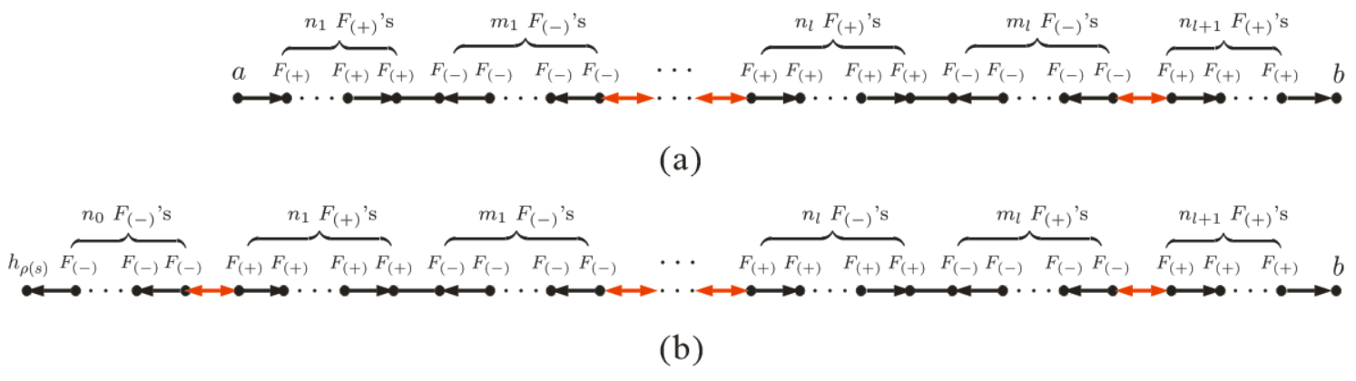
Figure 14: Graphs (a) and (b) correspond to chains led by $a\in\mathsf{H}\setminus\{h_{\rho(s)}\}$ and $h_{\rho(s)}$ defined by the refined graphic rule. A contraction of the form $(...\cdot F_{(+)})\cdot(F_{(-)}\cdot...)$ (in (a) and (b)) or $\epsilon_{a}\cdot(F_{(-)}\cdot...)$ (in (a)) provides a type-1 line, while a contraction of the form $(...\cdot F_{(-)})\cdot(F_{(+)}\cdot...)$ (in (a) and (b)), $k_{h_{\rho(s)}}\cdot F_{(+)}$ (in (b)), $F_{(-)}\cdot k_{b}$ (in (a) and (b)) or $k_{h_{\rho(s)}}\cdot k_{b}$ (in (b)) provides a type-3 line.

(i) When all strength tensors $F^{\mu\nu}$ are expressed by its definition eq. (2.3), a chain $\epsilon_{a}\cdot F_{i_{j}}\cdot...\cdot F_{i_{2}}\cdot F_{i_{1}}\cdot k_{b}$ ( $a\in\mathsf{H}\setminus\{h_{\rho(s)}\}$, $b$ belongs to a higher-weight chain or an element in $\{1,\dots,r-1\}$) is expanded as a sum of chains defined by the refined graphic rule. Each in the sum has the general form

$$\epsilon_{a}\mathop{\underbrace{\cdot(\mathop{\overbrace{F_{(+)}\cdot...\cdot F_{(+)}}}^{\text{$n_{1}$ $F_{(+)}$'s}}\cdot\mathop{\overbrace{F_{(-)}\cdot...\cdot F_{(-)}}}^{\text{$m_{1}$ $F_{(-)}$'s}})\cdot...\cdot(\mathop{\overbrace{F_{(+)}\cdot...\cdot F_{(+)}}}^{\text{$n_{l}$ $F_{(+)}$'s}}\cdot\mathop{\overbrace{F_{(-)}\cdot...\cdot F_{(-)}}}^{{\text{$m_{l}$ $F_{(-)}$'s}}})}}_{\text{$l$ sectors}}\cdot(\mathop{\overbrace{F_{(+)}\cdot...\cdot F_{(+)}}}^{\text{$n_{l+1}$ $F_{(+)}$'s}})\cdot k_{b},$$ (5.1)

where $F^{\mu\nu}_{(+)}\equiv k^{\mu}\epsilon^{\nu}$, $F^{\mu\nu}_{(-)}\equiv-\epsilon^{\mu}k^{\nu}$ correspond to the nodes Fig. 1 (a) and (b), $l\geq 0$. In the language of graphs, such a chain is characterized by Fig. 14 (a). If $l=0$, $n_{l+1=1}\geq 0$, the chain eq. (5.1) in this case has no type-3 line. If $l>0$, the value of integers $n_{i}$, $m_{i}$ satisfy $n_{1},n_{l+1}\geq 0$, $n_{i=2,\dots,l}>0$, $m_{i=1,\dots,l}>0$ and the chain in this case at least has one type-3 line.

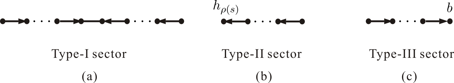
Figure 15: Three types of sectors of chains when all type-3 lines are removed

(ii) Similarly, the chain $k_{h_{\rho(s)}}\cdot F_{i_{j}}\cdot...\cdot F_{i_{1}}\cdot k_{b}$ ($b\in\{1,\dots,r-1\}$) can also be expanded as a sum of chains defined by the refined graphic rule. Each chain in the sum has the general form

$${\small k_{h_{\rho(s)}}\cdot(\mathop{\overbrace{F_{(-)}\cdot...\cdot F_{(-)}}}^{\text{$n_{0}$ $F_{(-)}$'s}})\mathop{\underbrace{\cdot(\mathop{\overbrace{F_{(+)}\cdot...\cdot F_{(+)}}}^{\text{$n_{1}$ $F_{(+)}$'s}}\cdot\mathop{\overbrace{F_{(-)}\cdot...\cdot F_{(-)}}}^{\text{$m_{1}$ $F_{(-)}$'s}})\cdot...\cdot(\mathop{\overbrace{F_{(+)}\cdot...\cdot F_{(+)}}}^{\text{$n_{l}$ $F_{(+)}$'s}}\cdot\mathop{\overbrace{F_{(-)}\cdot...\cdot F_{(-)}}}^{{\text{$m_{l}$ $F_{(-)}$'s}}})}}_{\text{$l$ sectors}}\cdot(\mathop{\overbrace{F_{(+)}\cdot...\cdot F_{(+)}}}^{\text{$n_{l+1}$ $F_{(+)}$'s}})\cdot k_{b},}$$

where $l\geq 0$. The value of integers $n_{i}$, $m_{i}$ satisfy $n_{0},n_{l+1}\geq 0$ (for $l\geq 0$), $n_{i=1,\dots,l}>0$, $m_{i=1,\dots,l}>0$ (for $l>0$). In the language of graphs, this chain is characterized by Fig. 14 (b). Since the arrow lines connected to the starting node $h_{\rho(s)}$ and the ending node $b$ in Fig. 14 point to opposite directions, there must be at least one type-3 line in Fig. 14 (b). In order to obtain the skeleton $\mathcal{F}^{\prime}$ of a graph $\mathcal{F}$, we delete all type-3 lines from $\mathcal{F}$. Then chains are divided into disjoint sectors in general. All sectors can be classified into the following types.

• Type-I sector: A sector containing a type-1 line (see Fig. 15 (a))  This sector can also have type-2 lines whose arrows point to the direction of the two end nodes of the type-1 line. Both types of chains Fig. 14 (a) and (b) can contain type-I sectors.

• Type-II sector: A sector only containing type-2 lines whose arrows point to the direction of the starting node of the chain (see Fig. 15 (b))  Only the highest-weight chain Fig. 14 (b) involve a type-II sector. The single node $h_{\rho(s)}$ with no line (on this chain) connected to it (i.e. Fig. 14 (b) with $n_{0}=0$) is considered as a special type-II sector.

• Type-III sector: A sector only containing type-2 lines whose arrows point to the direction of the ending node of a chain (see Fig. 15 (c))  Both types of chains Fig. 14 (a) and (b) contain type-III sectors. The single node $b$ with no line (on this chain) connected to it ( i.e. Fig. 14 (a) or (b) with $n_{l+1}=0$) is a special type-III sector.

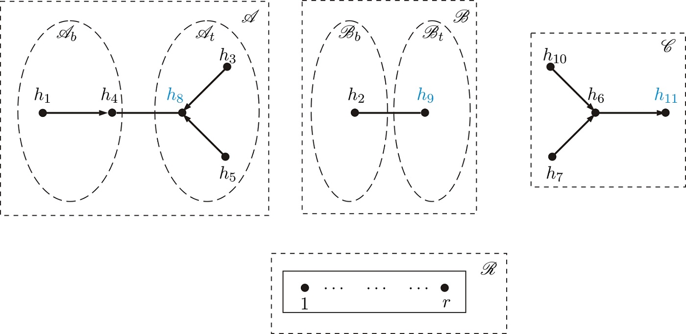
Figure 16: A skeleton consisting of four mutually disjoint components for the gauge invariance induced identity eq. (2.9) with $|\mathsf{H}|=11$. The reference order is chosen as $\mathsf{R}=\{h_{1},h_{2},\dots,h_{10},h_{11}\}$. Here, both $\mathscr{A}$ and $\mathscr{B}$ are type-I components. The kernel of $\mathscr{A}$ is given by the nodes $h_{4}$ and $h_{8}$ with a type-1 line between them (i.e. the factor $\epsilon_{h_{4}}\cdot\epsilon_{h_{8}}$), while the kernel of $\mathscr{B}$ is given by $h_{2}$ and $h_{9}$ with a type-1 line between them (i.e. $\epsilon_{h_{2}}\cdot\epsilon_{h_{9}}$). On each side of the component $\mathscr{A}$, the arrows of type-2 lines point to the corresponding end node of the kernel. The component $\mathscr{C}$ is the type-II component. The set $\mathscr{R}=\{1,\dots,r\}$ itself is the type-III component (Although only the elements $1$, …, $r-1$ can play as roots in the graphic rule, we also include the last element $r$ in the component $\mathscr{R}$ for convenience; A more general type-III componnet can involve type-II lines whose arrows pointing to roots).

According to the refined graphic rule, the highest-weight chain in a graph must be of the form Fig. 14 (b). This chain at least contains two mutually disjoint sectors: a type-II sector and a type-III sector. It can also have type-I sectors. The type-III sector of the highest-weight chain Fig. 14 (b) must end at a root $b\in\{1,\dots,r-1\}$ while all nodes on this chain can be ending nodes of type-III sectors of other chains. If we look at a chain of the form Fig. 14 (a), we find that the type-III sector of this chain can end at either a node of a higher-weight chain or a root $b\in\{1,\dots,r-1\}$, while any node on this chain can be the ending node of the type-III sector of a lower-weight chain. After putting all these sectors together, we conclude that a general skeleton is composed of the following types of components:

• Type-I component: component containing a type-1 line (see the $\mathscr{A}$ and $\mathscr{B}$ components in Fig. 16 for example)  Such a component consists of a type-I sector with possible type-III sectors attached to it. Each component of this type must have only one type-1 line in it and may also have type-2 lines pointing to the direction of the end nodes of the type-1 line. A type-I component can be reconstructed by connecting a type-1 line between two separate parts, each only contains type-2 lines. We define the part to which the highest-weight node of a type-I component belongs as the top side. The other part is called the bottom side. The type-1 line with its two end nodes together is defined as the kernel of this type-I component.

• Type-II component: the component containing the highest-weight graviton $h_{\rho(s)}$ (see the $\mathscr{C}$ components in Fig. 16 for example) This component consists of the type-II sector of the highest-weight chain with possible type-III sectors (belonging to other chains) attached on it. Apparently, type-II component involves only type-2 lines whose arrows point to the direction of the node $h_{\rho(s)}$.

• Type-III component: the component containing the set $\{1,\dots,r\}$ (see the $\mathscr{R}$ components in Fig. 16 for example)  This component is obtained by connecting possible type-III sectors to roots $b\in\{1,\dots,r-1\}$. Thus type-III components contains type-2 lines whose arrows point to the root set.

All the above three types of components can be considered as connected subgraphs where tree structures with only type-2 lines pointing to (i) the kernel (for type-I components), (ii) the highest-weight node $h_{\rho(s)}$ (for the type-II component) and (iii) roots (for the type-III component). If the highest-weight chain contains only one type-3 line in the original graph $\mathcal{F}$ while other chains do not have any type-3 line, the skeleton of $\mathcal{F}$ must consist of only two mutually disjoint components: the type-II and the type-III components (see Fig. 9 (a)-(h) for example).

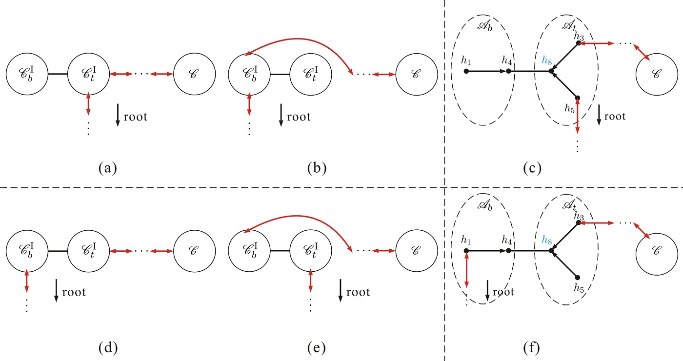
Figure 17: We use a circle to stand for an arbitrary component or the top or bottom side of a type-I component; A solid line between the top and bottom sides of a type-I component $\mathscr{C}^{\text{I}}$ stands for a type-1 line connecting two arbitrary nodes on the corresponding sides; A double arrow line between two distinct components stands for a type-3 line between two arbitrary nodes in corresponding components. Assume that $\mathscr{C}$ is the type-II component or a type-I component with a higher weight than $\mathscr{C}^{\text{I}}$. The graphs (a) and (b), in which a higher-weight chain passes through only one side of $\mathscr{C}^{\text{I}}$, are not allowed by the refined graphic rule because a chain cannot contain conflict arrow line towards root (e.g. the graph (c)). Thus if a chain passes through a component, it must pass through both sides of the component. In other words, the kernel of the component $\mathscr{C}^{\text{I}}$ must be on that chain (see the graphs (d) and (e) as well as the explicit example (f)).

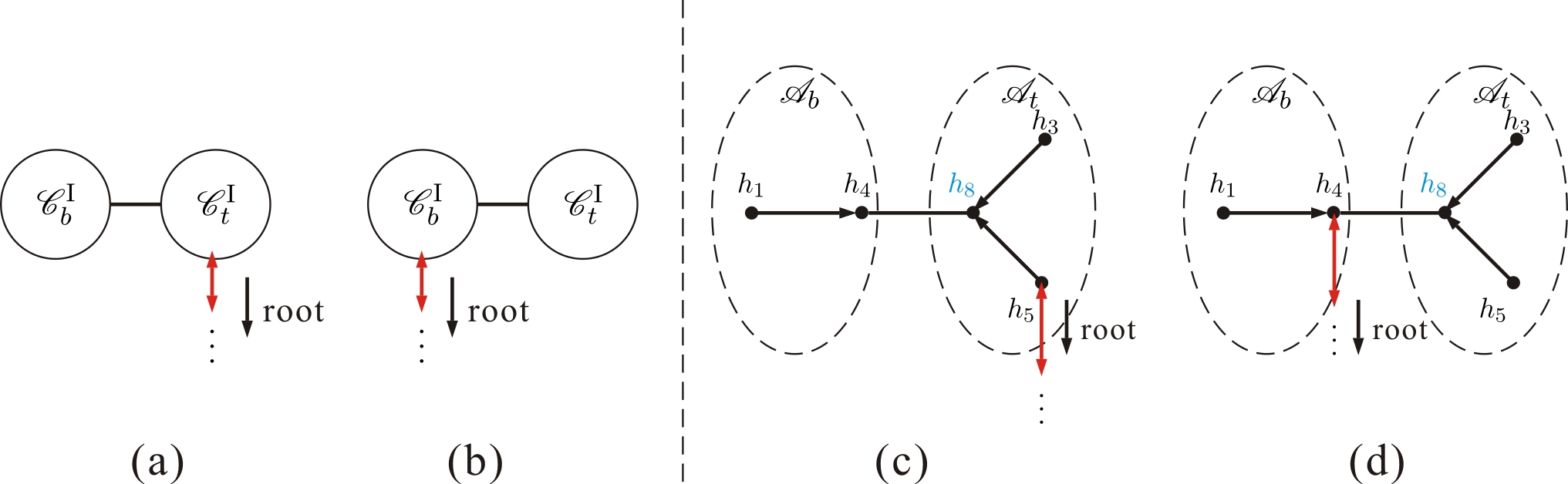
Figure 18: If there is a chain starting at the highest-weight node of a type-I component $\mathscr{C}^{\text{I}}$, this chain must contain the kernel of $\mathscr{C}^{\text{I}}$. In other words, the bottom-side end node of the kernel must be nearer to root than the top-side one. Thus the graph (b) (a more concrete example is given by (d)) is allowed but (a) (a more concrete example is given by (c)) is not allowed.

With the general structure of skeletons in hand, we will construct all graphs for an arbitrary skeleton in the rest of this section.

5.2 The construction of physical graphs for a given skeleton

Physical graphs corresponding to a given skeleton $\mathcal{F}^{\prime}$ can be obtained by connecting the disjoint components of $\mathcal{F}^{\prime}$ into a fully connected graph via type-3 lines. If the skeleton consists of $N$ disjoint components, the number of type-3 lines must be $N-1$. For the convenience of coming discussions, we define reference order $\mathsf{R}_{\mathscr{C}}$ of all type-I and type-II components in a skeleton by the relative order of their highest-weight nodes in $\mathsf{R}=\{h_{\rho(1)},h_{\rho(2)},\dots,h_{\rho(s)}\}$. For instance, the reference order of the components in Fig. 16 is $\mathsf{R}_{\mathscr{C}}=\{\mathscr{A},\mathscr{B},\mathscr{C}\}$. The position of a component in the ordered set $\mathsf{R}_{\mathscr{C}}$ is called the weight of the component. To construct all possible physical graphs containing a given skeleton $\mathcal{F}^{\prime}$, we should notice the following constraints from the refined graphic rule:

• Assume we have two components $\mathscr{C}^{\text{I}}$ and $\mathscr{C}$. Here, $\mathscr{C}^{\text{I}}$ is a type-I component while $\mathscr{C}$ is either the type-II or a type-I component whose weight is higher than that of $\mathscr{C}^{\text{I}}$. The structures shown in Fig. 17 (a) and (b), in which the chain led by the highest weight node in $\mathscr{C}$ passes through only a single side (the top or the bottom side) of the component $\mathscr{C}^{\text{I}}$ (via two type-3 lines), are forbidden. This is because if only the top (or bottom) side of $\mathscr{C}^{\text{I}}$ is passed through by the chain, there must exist an internal node which is attached by two conflict arrows on that chain (for example the node $h_{8}$ in Fig. 17.(c)). Such a structure is forbidden by the definition of the strength tensor $F^{\mu\nu}$. Therefore, only the graphs Fig. 17 (d) and (e) where the higher-weight chain pass through both sides of $\mathscr{C}^{\text{I}}$ are allowed (a more specific example is given by Fig. 17 (f)). In other words, if a chain of higher weight passes through a type-I component $\mathscr{C}^{\text{I}}$, the kernel of the component $\mathscr{C}^{\text{I}}$ (e.g. $\epsilon_{h_{4}}\cdot\epsilon_{h_{8}}$ for Fig. 17 (f)) must be on this chain.

• A chain, say $\mathbb{CH}_{1}$, starting at the highest-weight node of a type-I component $\mathscr{C}^{\text{I}}$ must pass through both sides of $\mathscr{C}^{\text{I}}$ (or equivalently the kernel of $\mathscr{C}^{\text{I}}$). If not (as shown by Fig. 18 (a) or a more explicit example Fig. 18 (c)), there must exist another chain, say $\mathbb{CH}_{2}$ which ends at some node $a\in\mathscr{C}^{\text{I}}_{t}\cap\mathbb{CH}_{1}$. The node $a$ plays as the ending node of $\mathbb{CH}_{2}$ but can only supply a $\epsilon$ to $\mathbb{CH}_{2}$, which apparently conflicts to the refined graphic rule.

With the help of these two constraints, we can construct all physical graphs for a given skeleton. Let us first illustrate this procedure by the skeleton Fig. 16.

5.2.1 An example: physical graphs for the skeleton Fig. 16

To construct all physical graphs containing the skeleton Fig. 16, we need to connect the four disjoint components $\mathscr{A}$, $\mathscr{B}$, $\mathscr{C}$ and $\mathscr{R}$ by three type-3 lines according to the refined graphic rule. All physical graphs for the skeleton Fig. 16 can be conveniently generated by constructing chains of components which reflect the structure of chains led by the highest-weight nodes in the corresponding components. Here we present two equivalent constructions of physical graphs for the skeleton Fig. 16.

Physical graphs for the skeleton Fig. 16: construction-1

Step-1  According to the graphic rule, there is always a chain which starts at the highest-weight node $h_{11}\in\mathscr{C}$ in a physical graph and ends at an element in $\mathscr{R}=\{1,\dots,r-1\}$. Corresponding to distinct configurations of the highest-weight chain (the chain led by the highest weight element $h_{11}$), we construct distinct chains of components which are led by $\mathscr{C}$ and ended at $\mathscr{R}$ as follows.

• Each graph where the highest-weight chain neither passes through $\mathscr{A}$ nor $\mathscr{B}$ contains a substructure where two nodes $a_{1}\in\mathscr{C}$ and $b_{1}\in\mathscr{R}$ are connected by a type-3 line. Such a substructure defines a chain of components: $\mathbb{CH}=[\mathscr{C},\mathscr{R}]$ (adjacent components on this chain are connected by a type-3 line).

• If $\mathscr{B}$ component is passed through by the highest-weight chain while $\mathscr{A}$ is not, there should exist $a_{1}\in\mathscr{C}$, $b_{1}\in\mathscr{B}$ connected by a type-3 line and $a_{2}\in\mathscr{B}$, $b_{2}\in\mathscr{R}$ by another one on this chain. Since a chain must pass through both sides of a type-I component, $b_{1}$ and $a_{2}$ should belong to distinct sides of $\mathscr{B}$, i.e. either $b_{1}\in\mathscr{B}_{t}$, $a_{2}\in\mathscr{B}_{b}$ or $b_{1}\in\mathscr{B}_{b}$, $a_{2}\in\mathscr{B}_{t}$ is satisfied. Correspondingly, a chain of components $\mathbb{CH}=[\mathscr{C},\mathscr{B}_{t}-\mathscr{B}_{b},\mathscr{R}]$ or $\mathbb{CH}=[\mathscr{C},\mathscr{B}_{b}-\mathscr{B}_{t},\mathscr{R}]$ is defined (Here a ‘$-$’ denotes the type-1 line between $\mathscr{B}_{t}$ and $\mathscr{B}_{b}$).

• Similarly with (ii), if $\mathscr{A}$ component is passed trough by the highest weight chain while $\mathscr{B}$ is not, we have $a_{1}\in\mathscr{C}$, $b_{1}\in\mathscr{A}$ connected by a type-3 line and $a_{2}\in\mathscr{A}$, $b_{2}\in\mathscr{R}$ by another. The nodes $b_{1}$ and $a_{2}$ can only belong to distinct sides of $\mathscr{A}$, thus we arrive two possible chains of components $\mathbb{CH}=[\mathscr{C},\mathscr{A}_{t}-\mathscr{A}_{b},\mathscr{R}]$ and $\mathbb{CH}=[\mathscr{C},\mathscr{A}_{b}-\mathscr{A}_{t},\mathscr{R}]$.

• If the highest-weight chain, which starts from $\mathscr{C}$ and ends at $\mathscr{R}$, passes through $\mathscr{A}$ and $\mathscr{B}$ in turn, each pair of nodes $(a_{i},b_{i})$ ($i=1,2,3,a_{1}\in\mathscr{C},b_{1},a_{2}\in\mathscr{A},b_{2},a_{3}\in\mathscr{B},b_{3}\in\mathscr{R}$) is connected by a type-3 line. In addition, $b_{1}$, $a_{2}$ ($b_{2}$, $a_{3}$) must belong to distinct sides of the component $\mathscr{A}$ ($\mathscr{B}$). Hence we obtain the following four chains of components

  $$\mathbb{CH}=[\mathscr{C},\mathscr{B}_{t}-\mathscr{B}_{b},\mathscr{A}_{t}-\mathscr{A}_{b},\mathscr{R}]:~{}\text{Fig.~{}\ref{Fig:Figure14}}(a),\mathbb{CH}=[\mathscr{C},\mathscr{B}_{t}-\mathscr{B}_{b},\mathscr{A}_{b}-\mathscr{A}_{t},\mathscr{R}]:~{}\text{Fig.~{}\ref{Fig:Figure14}}(b)$$

  $$\mathbb{CH}=[\mathscr{C},\mathscr{B}_{b}-\mathscr{B}_{t},\mathscr{A}_{t}-\mathscr{A}_{b},\mathscr{R}]:~{}\text{Fig.~{}\ref{Fig:Figure14}}(c),\mathbb{CH}=[\mathscr{C},\mathscr{B}_{b}-\mathscr{B}_{t},\mathscr{A}_{b}-\mathscr{A}_{t},\mathscr{R}]:~{}\text{Fig.~{}\ref{Fig:Figure14}}(d).$$ (5.3)

• If the highest-weight chain passes trough $\mathscr{B}$ and $\mathscr{A}$ in turn, we just exchange the roles of components $\mathscr{A}$ and $\mathscr{B}$ in the previous case. Then the following chains of components are obtained

  $$\mathbb{CH}=[\mathscr{C},\mathscr{A}_{t}-\mathscr{A}_{b},\mathscr{B}_{t}-\mathscr{B}_{b},\mathscr{R}]:~{}\text{Fig.~{}\ref{Fig:Figure14}}(e),\mathbb{CH}=[\mathscr{C},\mathscr{A}_{t}-\mathscr{A}_{b},\mathscr{B}_{b}-\mathscr{B}_{t},\mathscr{R}]:~{}\text{Fig.~{}\ref{Fig:Figure14}}(f)$$

  $$\mathbb{CH}=[\mathscr{C},\mathscr{A}_{b}-\mathscr{A}_{t},\mathscr{B}_{t}-\mathscr{B}_{b},\mathscr{R}]:~{}\text{Fig.~{}\ref{Fig:Figure14}}(g),\mathbb{CH}=[\mathscr{C},\mathscr{A}_{b}-\mathscr{A}_{t},\mathscr{B}_{b}-\mathscr{B}_{t},\mathscr{R}]:~{}\text{Fig.~{}\ref{Fig:Figure14}}(h).$$ (5.4)

Having constructed a chain of components $\mathbb{CH}$ starting from $\mathscr{C}$ and ending at $\mathscr{R}$, we redefine the reference order $\mathsf{R}_{\mathscr{C}}$ by deleting the components which have been used, i.e, $\mathsf{R}_{\mathscr{C}}\to\mathsf{R}_{\mathscr{C}}^{\prime}=\mathsf{R}_{\mathscr{C}}\setminus\mathbb{CH}$. For the cases (iv) and (v), the ordered set $\mathsf{R}_{\mathscr{C}}$ have been clear up, thus the procedure is terminated. For the cases (i), (ii) and (iii), we should further construct other chains of components in the next step.

Step-2  Pick out the highest-weight component from the redefined $\mathsf{R}_{\mathscr{C}}$ (if it is not empty) and construct a new chain of components towards a component on $\mathbb{CH}$ which have been constructed previously.

• Based on the chain $\mathbb{CH}=[\mathscr{C},\mathscr{R}]$, the reference order $\mathsf{R}_{\mathscr{C}}$ is redefined as $\mathsf{R}_{\mathscr{C}}^{\prime}=\{\mathscr{A},\mathscr{B}\}$ where the highest-weight component is $\mathscr{B}$. The chain led by the highest-weight node in $\mathscr{B}$ can directly ends at a node in $\mathscr{C}\oplus\mathscr{R}$ ($\oplus$ denotes disjoint union) or passes through the component $\mathscr{A}$. For the former case, there exist two nodes on the chain $a^{\prime}_{1}\in\mathscr{B}$ and $b^{\prime}_{1}\in\mathscr{C}\oplus\mathscr{R}$ which are connected by a type-3 line. Considering that the bottom-side end node of the kernel of $\mathscr{B}$ is nearer to roots than the top-side one, possible new chains of components are constructed as

  $$\mathbb{CH}^{\prime}=[\mathscr{B}_{t}-\mathscr{B}_{b},\mathscr{C}\text{~{}or~{}}\mathscr{R}].$$ (5.5)

  For the latter case, one can find two pairs of nodes $a^{\prime}_{1}$, $b^{\prime}_{1}$ ($a^{\prime}_{1}\in\mathscr{B}$, $b^{\prime}_{1}\in\mathscr{A}$) and $a^{\prime}_{2}$, $b^{\prime}_{2}$ ($a^{\prime}_{2}\in\mathscr{A}$, $b^{\prime}_{2}\in\mathscr{C}~{}\text{or}~{}\mathscr{R}$), each pair is connected by a type-3 line. Since $b^{\prime}_{1}$ and $a^{\prime}_{2}$ must live in distinct sides of $\mathscr{A}$, possible chains of components are constructed as

  $$\mathbb{CH}^{\prime}=[\mathscr{B}_{t}-\mathscr{B}_{b},\mathscr{A}_{t}-\mathscr{A}_{b},\mathscr{C}],~{}~{}~{}\mathbb{CH}^{\prime}=[\mathscr{B}_{t}-\mathscr{B}_{b},\mathscr{A}_{t}-\mathscr{A}_{b},\mathscr{R}],$$

  $$\mathbb{CH}^{\prime}=[\mathscr{B}_{t}-\mathscr{B}_{b},\mathscr{A}_{b}-\mathscr{A}_{t},\mathscr{C}],~{}~{}~{}\mathbb{CH}^{\prime}=[\mathscr{B}_{t}-\mathscr{B}_{b},\mathscr{A}_{b}-\mathscr{A}_{t},\mathscr{R}].$$ (5.6)

  Each of the above four possible chains of components together with the chain $\mathbb{CH}=[\mathscr{C},\mathscr{R}]$ constructed by step-1 (i) forms a full physical graph (see Fig. 29 (e), (g), (f) or (h)).

• The reference order of components defined in step-1 (ii) is $\mathsf{R}_{\mathscr{C}}^{\prime}=\{\mathscr{A}\}$. The chain led by the highest-weight node in $\{\mathscr{A}\}$ must ends at a node in $\mathscr{C}\oplus\mathscr{B}\oplus\mathscr{R}$. Thus this chain contains a node $a^{\prime}_{1}\in\mathscr{A}$ and a node $b^{\prime}_{1}\in\mathscr{C}\oplus\mathscr{B}\oplus\mathscr{R}$ which are connected with each other by a type-3 line. Since the chain led by the highest-weight node $h_{8}$ in $\mathscr{A}$ have to pass through both top and bottom sides of $\mathscr{A}$, $a^{\prime}_{1}$ must be in $\mathscr{A}_{t}$. Possible chains of components are defined as

  $$\mathbb{CH}^{\prime}=[\mathscr{A}_{t}-\mathscr{A}_{b},\mathscr{C}\text{~{}or~{}}\mathscr{B}\text{~{}or~{}}\mathscr{R}].$$ (5.7)

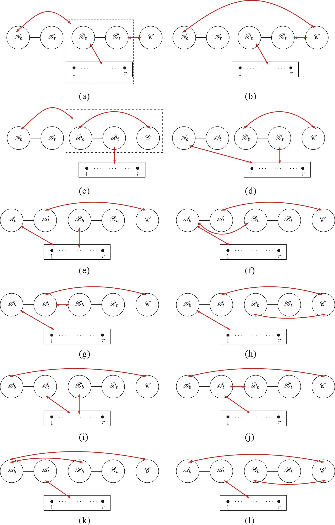
Figure 30: Physical graphs for the skeleton Fig. 16 by construction-1: part 2.

  This chain together with the chains $\mathbb{CH}=[\mathscr{C},\mathscr{B}_{t}-\mathscr{B}_{b},\mathscr{R}]$ and $\mathbb{CH}=[\mathscr{C},\mathscr{B}_{b}-\mathscr{B}_{t},\mathscr{R}]$ constructed in step-1 (ii) provides full physical graphs Fig. 30 (a), (b) and Fig. 30 (c), (d), respectively.

• The reference order of components defined in step-1 (iii) is $\mathsf{R}_{\mathscr{C}}^{\prime}=\{\mathscr{B}\}$. Similarly with (ii) in this step, one can construct a chain of component led by $\mathscr{B}$ towards the components that have been used in step-1 (iii):

  $$\mathbb{CH}^{\prime}=[\mathscr{B}_{t}-\mathscr{B}_{b},\mathscr{C}\text{~{}or~{}}\mathscr{A}\text{~{}or~{}}\mathscr{R}],$$ (5.8)

  which reflects that a chain led by the highest-weight node $h_{9}$ ends at a node in $\mathscr{C}\oplus\mathscr{A}\oplus\mathscr{R}$. Together with the chains $\mathbb{CH}=[\mathscr{C},\mathscr{A}_{t}-\mathscr{A}_{b},\mathscr{R}]$ and $\mathbb{CH}=[\mathscr{C},\mathscr{A}_{b}-\mathscr{A}_{t},\mathscr{R}]$ produced in step-1 (iii), this chain of components provides the full graphs Fig. 30 (e), (f), (g), (h) and Fig. 30 (i), (j), (k), (l), respectively.

Having constructed all chains for the second step, we redefine the reference order $\mathsf{R}_{\mathscr{C}}$ of the components again by removing the components which have been used in step-2. This procedure is terminated for the cases with empty redefined $\mathsf{R}_{\mathscr{C}}$ and all graphs completed in this step are given by Fig. 29.(e)-(h) and Fig. 30.(a)-(l). Then only the $\mathsf{R}_{\mathscr{C}}=\{\mathscr{A}\}$ which is redefined after the construction of the chain $\mathbb{CH}^{\prime}=[\mathscr{B}_{t}-\mathscr{B}_{b},\mathscr{C}\text{~{}or~{}}\mathscr{R}]$ in step-2 (i) is nonempty and requires a further step.

Step-3  The highest-weight component in the redefined reference order $\mathsf{R}_{\mathscr{C}}=\{\mathscr{A}\}$, which is based on the chain $\mathbb{CH}^{\prime}=[\mathscr{B}_{t}-\mathscr{B}_{b},\mathscr{C}\text{~{}or~{}}\mathscr{R}]$ constructed in step-2 (i), is $\mathscr{A}$. There must be a node $a^{\prime\prime}_{1}\in\mathscr{A}$ and a node $b^{\prime\prime}_{1}\in\mathscr{B}\oplus\mathscr{C}\oplus\mathscr{R}$ which are connected with each other by a type-3 line on this chain. This structure corresponds to a chain of components

$$\mathbb{CH}^{\prime\prime}=[\mathscr{A},\mathscr{B}\text{~{}or~{}}\mathscr{C}\text{~{}or~{}}\mathscr{R}].$$ (5.9)

The chains of components $\mathbb{CH}=[\mathscr{C},\mathscr{R}]$ and $\mathbb{CH}^{\prime}=[\mathscr{B}_{t}-\mathscr{B}_{b},\mathscr{C}\text{~{}or~{}}\mathscr{R}]$ respectively constructed by step-1 (i) and step-2 (i) together with the above chain produce full graphs Fig. 29 (a)-(d).

All graphs constructed by the above steps with all possible choices of end nodes of type-3 lines together form the full set of physical graphs (graphs constructed by the refined graphic rule) containing the skeleton Fig. 16.

Physical graphs for the skeleton Fig. 16: construction-2

Physical graphs for a given skeleton can be constructed in a distinct way. We define the reference order of all type-I components by removing the type-II component from $\mathsf{R}_{\mathscr{C}}$: $\mathsf{R}^{\,\text{I}}_{\mathscr{C}}\equiv\mathsf{R}_{\mathscr{C}}\setminus\mathscr{C}=\{\mathscr{A},\mathscr{B}\}$. We also define the upper block $\mathscr{U}$ and lower block $\mathscr{L}$ of a graph by the maximally connected graphs (constructed in an intermediate step) that contain the type-II component $\mathscr{C}$ and the type-III component $\mathscr{R}$, respectively. All physical graphs can be obtained by the following steps.

Step-1   At the beginning $\mathscr{U}=\mathscr{C}$ and $\mathscr{L}=\mathscr{R}$. We consider the nodes in $\mathscr{U}$ and in $\mathscr{L}$ (except the node $r$) as two distinct sets of roots. Pick out the highest-weight component $\mathscr{B}$ from $\mathsf{R}^{\,\text{I}}_{\mathscr{C}}$ and construct a chain of component which starts from $\mathscr{B}$ towards either $\mathscr{U}$ or $\mathscr{L}$. Note that the bottom-side end node of the kernel of $\mathscr{B}$ must be nearer to root than the top-side one. According to whether $\mathscr{A}$ component is on this chain and whether the chain ends at the upper block $\mathscr{U}$ or lower block $\mathscr{L}$, we construct the following possible configurations:

$$\text{(i)}.~{}~{}~{}\mathscr{U}\to\mathscr{U}^{\prime}=[\mathscr{B}_{t}-\mathscr{B}_{b},\mathscr{C}],~{}\mathscr{L}\to\mathscr{L}^{\prime}=\mathscr{R};~{}~{}~{}~{}\text{(ii)}.~{}\mathscr{U}\to\mathscr{U}^{\prime}=\mathscr{C},~{}\mathscr{L}\to\mathscr{L}^{\prime}=[\mathscr{B}_{t}-\mathscr{B}_{b},\mathscr{R}];~{}~{}$$ (5.10)

$$\text{(iii)}.~{}\,\mathscr{U}\to\mathscr{U}^{\prime}=[\mathscr{B}_{t}-\mathscr{B}_{b},\mathscr{A}_{t}-\mathscr{A}_{b},\mathscr{C}],~{}\mathscr{L}\to\mathscr{L}^{\prime}=\mathscr{R};$$

$$\text{(iv)}.~{}\,\mathscr{U}\to\mathscr{U}^{\prime}=[\mathscr{B}_{t}-\mathscr{B}_{b},\mathscr{A}_{b}-\mathscr{A}_{t},\mathscr{C}],~{}\mathscr{L}\to\mathscr{L}^{\prime}=\mathscr{R};$$

$$\text{(v)}.~{}~{}\,\mathscr{U}\to\mathscr{U}^{\prime}=\mathscr{C},~{}\mathscr{L}\to[\mathscr{B}_{t}-\mathscr{B}_{b},\mathscr{A}_{t}-\mathscr{A}_{b},\mathscr{R}];\text{(vi)}.~{}\mathscr{U}\to\mathscr{U}^{\prime}=\mathscr{C},~{}\mathscr{L}\to[\mathscr{B}_{t}-\mathscr{B}_{b},\mathscr{A}_{b}-\mathscr{A}_{t},\mathscr{R}],$$

where we have redefined the upper and lower blocks by the new maximally connected graphs $\mathscr{U}^{\prime}$ and $\mathscr{L}^{\prime}$ that contain $\mathscr{C}$ and $\mathscr{R}$ respectively. Redefine $\mathsf{R}^{\,\text{I}}_{\mathscr{C}}$ by removing the components which have been used on the chain led by $\mathscr{B}$. In (iii), (iv), (v) and (vi) of eq. (5.10), the chain led by $\mathscr{B}$ passes through $\mathscr{A}$ (the last three lines of eq. (5.10)) and the redefined $\mathsf{R}^{\,\text{I}}_{\mathscr{C}}$ becomes empty (thus this process is terminated). Contrarily, in (i) and (ii), the component $\mathscr{A}$ is not on the chain led by $\mathscr{B}$ and the redefined $\mathsf{R}^{\,\text{I}}_{\mathscr{C}}$ is a nonempty set $\{\mathscr{A}\}$. Thus we have to turn to the next step for (i) and (ii).

Step-2   Since the ordered set $\mathsf{R}^{\,\text{I}}_{\mathscr{C}}$ redefined after (i) and (ii) in the previous step is an nonempty one $\{\mathscr{A}\}$, we need to construct chains, which start from the component $\mathscr{A}$, towards either the upper block $\mathscr{U}^{\prime}$ or the lower block $\mathscr{L}^{\prime}$ (which is defined in (i) and (ii) (see eq. (5.10))). Based on eq. (5.10) (i) and (ii), possible structures are further constructed as follows

$$\text{(i)}.~{}~{}\mathscr{U}\to\mathscr{U}^{\prime\prime}=[\mathscr{A}_{t}-\mathscr{A}_{b},\mathscr{U}^{\prime}],~{}~{}\mathscr{L}\to\mathscr{L}^{\prime\prime}=\mathscr{L}^{\prime};$$

$$\text{(ii)}.~{}\mathscr{U}\to\mathscr{U}^{\prime\prime}=\mathscr{U}^{\prime},~{}~{}~{}~{}~{}~{}~{}~{}~{}~{}~{}~{}~{}~{}~{}\,\mathscr{L}\to\mathscr{L}^{\prime\prime}=[\mathscr{A}_{t}-\mathscr{A}_{b},\mathscr{L}^{\prime}],$$ (5.11)

where $\mathscr{U}^{\prime}$ and $\mathscr{L}^{\prime}$ are the upper and lower blocks defined in either eq. (5.10) (i) or eq. (5.10) (ii). Redefine the ordered set $\mathsf{R}^{\,\text{I}}_{\mathscr{C}^{\prime}}=\{\mathscr{A}\}$ obtained in the previous step by removing $\mathscr{A}$. Then $\mathsf{R}^{\,\text{I}}_{\mathscr{C}^{\prime}}$ becomes empty.

Step-3   After the previous steps, the ordered set $\mathsf{R}^{\text{I}}_{\mathscr{C}^{\prime}}$ becomes empty and all graphs consists of only two disjoint blocks, the redefined $\mathscr{U}$ and $\mathscr{L}$ which will be called the final upper and lower blocks, respectively. Now we connect two nodes correspondingly belonging to the final blocks $\mathscr{U}$ and $\mathscr{L}-\{r\}$, by a type-3 line and make sure the chain led by the component $\mathscr{C}$ cannot only pass through a single side of any type-I component (i.e. graphs with structures Fig. 17 (a) and (b) are excluded). The graph then becomes a connected one. Since the highest-weight node $h_{11}$ belongs to $\mathscr{U}$ while all roots $\{1,\dots,r-1\}$ are contained by $\mathscr{L}-\{r\}$, the highest-weight chain that starts from $h_{11}$ and ends at an element in $\{1,\dots,r-1\}$ is constructed in this step. Finally, all graphs constructed in this way are presented by Fig. 32.(a1), (a2), (a3), (a4), Fig. 33.(a1), (b1), (c1), (d1) and Fig. 34.(a1), (b1), (c1), (d1).

The equivalence between the two constructions

The first version of construction naturally inherits the refined graphic rule because a chain of components is just constructed by keeping track of the chain led by the highest weight node in the starting component. We need to verify that the second construction also provides the same physical graphs with the first approach. The explicit correspondence between the second and the first construction is following

Fig. 32 (a1)-(c1) $$\Leftrightarrow \text{Fig.~{}\ref{Fig:Figure12} (a)},~{}\text{Fig.~{}\ref{Fig:Figure13} (a),(e)},~{}\text{Fig.~{}\ref{Fig:Figure14} (e)};$$

Fig. 32 (d1) $$\Leftrightarrow \text{Fig.~{}\ref{Fig:Figure12} (b)},~{}\text{Fig.~{}\ref{Fig:Figure13} (b),(i)},~{}\text{Fig.~{}\ref{Fig:Figure14} (g)};$$

Fig. 33 (a1) $$\Leftrightarrow \text{Fig.~{}\ref{Fig:Figure12} (d)},~{}\text{Fig.~{}\ref{Fig:Figure13} (d),(h)},~{}\text{Fig.~{}\ref{Fig:Figure14} (c)};$$

Fig. 33 (b1)-(d1) $$\Leftrightarrow \text{Fig.~{}\ref{Fig:Figure12} (c)},~{}\text{Fig.~{}\ref{Fig:Figure13} (c),(l)},~{}\text{Fig.~{}\ref{Fig:Figure14} (d)};$$

Fig. 34 (a1) $$\Leftrightarrow \text{Fig.~{}\ref{Fig:Figure12} (e)},~{}\text{Fig.~{}\ref{Fig:Figure13} (g)},~{}\text{Fig.~{}\ref{Fig:Figure14} (a)};$$

Fig. 34 (b1) $$\Leftrightarrow \text{Fig.~{}\ref{Fig:Figure12} (f)},~{}\text{Fig.~{}\ref{Fig:Figure13} (k)},~{}\text{Fig.~{}\ref{Fig:Figure14} (b)};$$

Fig. 34 (c1) $$\Leftrightarrow \text{Fig.~{}\ref{Fig:Figure12} (g)},~{}\text{Fig.~{}\ref{Fig:Figure13} (j)},~{}\text{Fig.~{}\ref{Fig:Figure14} (h)};$$

Fig. 34 (d1) $$\Leftrightarrow \text{Fig.~{}\ref{Fig:Figure12} (h)},~{}\text{Fig.~{}\ref{Fig:Figure13} (f)},~{}\text{Fig.~{}\ref{Fig:Figure14} (f)}.$$ (5.12)

Thus the two constructions for this example precisely match with each other.

5.2.2 General rules for the construction of physical graphs

Inspired by the two constructions of physical graphs for the skeleton Fig. 16, we propose two distinct rules for constructing all physical graphs for an arbitrary skeleton. We will prove that these two rules in fact provide the same physical graphs.

Rule-1

As we have already stated in section 5.1, each skeleton $\mathcal{F}\,^{\prime}$ in eq. (3.5) at least contains a type-II component $\mathscr{C}^{\text{II}}$ and a type-III component $\mathscr{C}^{\text{III}}$. Moreover, $N$ type-I components $\mathscr{C}_{1}^{\text{I}}$, $\mathscr{C}_{2}^{\text{I}}$, …, $\mathscr{C}_{N}^{\text{I}}$ may also be involved. To construct all physical graphs for a skeleton with $N+2$ components, we should connect these components together via $N+1$ type-3 lines properly. This can be achieved by the following steps.

Step-1 Assuming that the reference order of all type-I and type-II components is given by $\mathsf{R}_{\mathscr{C}}=\{\mathscr{C}_{1}^{\text{I}},\mathscr{C}_{2}^{\text{I}},\dots,\mathscr{C}_{N}^{\text{I}},\mathscr{C}^{\text{II}}\}$, we pick out the type-II component $\mathscr{C}^{\text{II}}$ (the highest-weight component) as well as arbitrary type-I components $\mathscr{C}_{a_{1}}^{\text{I}}$, $\mathscr{C}_{a_{2}}^{\text{I}}$, …, $\mathscr{C}_{a_{i}}^{\text{I}}$ (not necessary to preserve the relative order in $\mathsf{R}_{\mathscr{C}}$) and construct a chain $\mathbb{CH}$, whose starting component is $\mathscr{C}^{\text{II}}$ and internal components are $\mathscr{C}_{a_{1}}^{\text{I}}$, $\mathscr{C}_{a_{2}}^{\text{I}}$, …, $\mathscr{C}_{a_{i}}^{\text{I}}$, towards $\mathscr{C}^{\text{III}}$:

$$\mathbb{CH}=\left[\mathscr{C}^{\text{II}},\left(\mathscr{C}_{a_{i}}^{\text{I}}\right)_{t\,(\text{or~{}}b)}-\left(\mathscr{C}_{a_{i}}^{\text{I}}\right)_{b\,(\text{or~{}}t)},\dots,\left(\mathscr{C}_{a_{1}}^{\text{I}}\right)_{t\,(\text{or~{}}b)}-\left(\mathscr{C}_{a_{1}}^{\text{I}}\right)_{b\,(\text{or~{}}t)},\mathscr{C}^{\text{III}}\right].$$ (5.13)

Redefine the reference order by $\mathsf{R}_{\mathscr{C}}\to\mathsf{R}_{\mathscr{C}}^{\prime}\equiv\mathsf{R}_{\mathscr{C}}\setminus\left\{\mathscr{C}^{\text{II}},\mathscr{C}_{a_{1}}^{\text{I}},\mathscr{C}_{a_{2}}^{\text{I}},\dots,\mathscr{C}_{a_{i}}^{\text{I}}\right\}$.

Step-2 After the redefinition in the previous step, the ordered set $\mathsf{R}_{\mathscr{C}}=\mathsf{R}_{\mathscr{C}}^{\prime}$ only consists of type-I components. Now we pick out the highest-weight component, say $\mathscr{C}_{a_{i^{\prime}}^{\prime}}^{\text{I}}$ as well as arbitrary type-I components $\mathscr{C}_{a_{1}^{\prime}}^{\text{I}}$, …, $\mathscr{C}_{a_{i^{\prime}}^{\prime}}^{\text{I}}$ from $\mathsf{R}_{\mathscr{C}}^{\prime}$ and construct a chain $\mathbb{CH}^{\prime}$ towards a component $\mathscr{C}\in\bigl{\{}\mathscr{C}^{\text{II}},\mathscr{C}_{a_{1}}^{\text{I}},\mathscr{C}_{a_{2}}^{\text{I}},\dots,\mathscr{C}_{a_{i}}^{\text{I}},\mathscr{C}^{\text{III}}\bigr{\}}$, which has been used in the previous step, as follows:

$$\mathbb{CH}^{\prime}=\left[\bigl{(}\mathscr{C}_{a_{i^{\prime}}^{\prime}}^{\text{I}}\bigr{)}_{t\,(\text{or~{}}b)}-\bigl{(}\mathscr{C}_{a_{i^{\prime}}^{\prime}}^{\text{I}}\bigr{)}_{b\,(\text{or~{}}t)},\bigl{(}\mathscr{C}_{a_{i^{\prime}-1}^{\prime}}^{\text{I}}\bigr{)}_{t\,(\text{or~{}}b)}-\bigl{(}\mathscr{C}_{a_{i^{\prime}-1}^{\prime}}^{\text{I}}\bigr{)}_{b\,(\text{or~{}}t)},\dots,\bigl{(}\mathscr{C}_{a_{1}^{\prime}}^{\text{I}}\bigr{)}_{t\,(\text{or~{}}b)}-\bigl{(}\mathscr{C}_{a_{1}^{\prime}}^{\text{I}}\bigr{)}_{b\,(\text{or~{}}t)}\leftrightarrow\mathscr{C}\right].$$

Redefine the reference order by $\mathsf{R}_{\mathscr{C}}\to\mathsf{R}_{\mathscr{C}}^{\prime\prime}\equiv\mathsf{R}_{\mathscr{C}}^{\prime}\setminus\{\mathscr{C}_{a_{1}^{\prime}}^{\text{I}},\mathscr{C}_{a_{2}^{\prime}}^{\text{I}},\dots,\mathscr{C}_{a_{i^{\prime}}^{\prime}}^{\text{I}}\}$.

Step-3 Repeat the above steps. In each step, construct a chain, whose starting component is the highest-weight one in $\mathsf{R}_{\mathscr{C}}$ redefined by the previous step, towards an arbitrary component which has been used in the previous steps. Then redefine $\mathsf{R}_{\mathscr{C}}$ by removing the starting and internal components which have been used in this step. This procedure is terminated till the ordered set $\mathsf{R}_{\mathscr{C}}$ becomes empty. We obtain a physical graph containing the skeleton $\mathcal{F}\,^{\prime}$.

All graphs (all possible chain structures of components and all possible choices of the end nodes of each type-3 lines) together form the set of all physical graphs $\mathcal{F}$ for the skeleton $\mathcal{F}\,^{\prime}$.

Rule-2

Inspired by the second construction of physical graphs for the skeleton Fig. 16, we propose the following rule which is essentially equivalent with rule-1.

Step-1 Define the upper and lower blocks $\mathscr{U}$ and $\mathscr{L}$ by the maximally connected graphs $\mathscr{C}^{\text{II}}$ and $\mathscr{C}^{\text{III}}$ that contains the highest weight node $h_{\rho(h)}$ and the elements $\{1,\dots,r-1\}$ respectively and define the reference order of all type-I components by $\mathsf{R}^{\,\text{I}}_{\mathscr{C}}\equiv\mathsf{R}_{\mathscr{C}}\setminus\mathscr{C}^{\text{II}}=\{\mathscr{C}_{1}^{\text{I}},\mathscr{C}_{2}^{\text{I}},\dots,\mathscr{C}_{N}^{\text{I}}\}$. We construct a chain, whose starting component is the highest-weight one in $\mathsf{R}^{\,\text{I}}_{\mathscr{C}}$ (i.e., $\mathscr{C}_{N}^{\text{I}}$) and internal components are arbitrarily chosen as $\mathscr{C}_{a_{1}}^{\text{I}}$, $\mathscr{C}_{a_{2}}^{\text{I}}$, …, $\mathscr{C}_{a_{i}}^{\text{I}}$ (not necessary in the relative order in $\mathsf{R}^{\,\text{I}}_{\mathscr{C}}$), towards either the upper block $\mathscr{U}$ or the lower block $\mathscr{L}$. Correspondingly, we get two possible structures

$$\text{(i)}. \mathscr{U}\to\mathscr{U}^{\prime}=\bigl{[}\big{(}\mathscr{C}_{N}^{\text{I}}\bigr{)}_{t}-\big{(}\mathscr{C}_{N}^{\text{I}}\bigr{)}_{b},\big{(}\mathscr{C}_{a_{i}}^{\text{I}}\bigr{)}_{t\,(\text{or~{}}b)}-\big{(}\mathscr{C}_{a_{i}}^{\text{I}}\bigr{)}_{b\,(\text{or~{}}t)},\dots,\big{(}\mathscr{C}_{a_{1}}^{\text{I}}\bigr{)}_{t\,(\text{or~{}}b)}-\big{(}\mathscr{C}_{a_{1}}^{\text{I}}\bigr{)}_{b\,(\text{or~{}}t)},\mathscr{C}^{\text{II}}\bigr{]},$$

$$\mathscr{L}\to\mathscr{L}^{\prime}=\mathscr{C}^{\text{III}};$$

$$\text{(ii)}. \mathscr{U}\to\mathscr{U}^{\prime}=\mathscr{C}^{\text{II}},$$ (5.15)

$$\mathscr{L}\to\mathscr{L}^{\prime}=\bigl{[}\big{(}\mathscr{C}_{N}^{\text{I}}\bigr{)}_{t}-\big{(}\mathscr{C}_{N}^{\text{I}}\bigr{)}_{b},\big{(}\mathscr{C}_{a_{i}}^{\text{I}}\bigr{)}_{t\,(\text{or~{}}b)}-\big{(}\mathscr{C}_{a_{i}}^{\text{I}}\bigr{)}_{b\,(\text{or~{}}t)},\dots,\big{(}\mathscr{C}_{a_{1}}^{\text{I}}\bigr{)}_{t\,(\text{or~{}}b)}-\big{(}\mathscr{C}_{a_{1}}^{\text{I}}\bigr{)}_{b\,(\text{or~{}}t)},\mathscr{C}^{\text{III}}\bigr{]}.$$

Redefine $\mathsf{R}_{\mathscr{C}}^{\,\text{I}}$ by ${\mathsf{R}_{\mathscr{C}}^{\,\text{I}}}^{\prime}=\mathsf{R}_{\mathscr{C}}^{\,\text{I}}\setminus\{\mathscr{C}_{N}^{\text{I}},\mathscr{C}_{a_{1}}^{\text{I}},\dots,\mathscr{C}_{a_{i}}^{\text{I}}\}$, $\mathscr{U}$ and $\mathscr{L}$ by the new obtained upper and lower blocks $\mathscr{U}^{\prime}$ and $\mathscr{L}^{\prime}$ respectively.

Step-2 Pick out the highest-weight component $\mathscr{C}_{a^{\prime}_{i^{\prime}}}^{\text{I}}$ and arbitrary components $\mathscr{C}_{a^{\prime}_{1}}^{\text{I}}$, …, $\mathscr{C}_{a^{\prime}_{i^{\prime}-1}}^{\text{I}}$ from ${\mathsf{R}_{\mathscr{C}}^{\,\text{I}}}^{\prime}$ defined in the previous step. Construct a chain, whose starting component is $\mathscr{C}_{a^{\prime}_{i^{\prime}}}^{\text{I}}$ and internal components are $\mathscr{C}_{a^{\prime}_{1}}^{\text{I}}$, …, $\mathscr{C}_{a^{\prime}_{i^{\prime}-1}}^{\text{I}}$, towards either the upper block $\mathscr{U}^{\prime}$ or the lower one $\mathscr{L}^{\prime}$:

$$(i). \mathscr{U}\to\mathscr{U}^{\prime\prime}=\bigl{[}\big{(}\mathscr{C}_{a_{i^{\prime}}^{\prime}}^{\text{I}}\bigr{)}_{t}-\big{(}\mathscr{C}_{a_{i^{\prime}}^{\prime}}^{\text{I}}\bigr{)}_{b},\big{(}\mathscr{C}_{a_{i^{\prime}-1}^{\prime}}^{\text{I}}\bigr{)}_{t\,(\text{or~{}}b)}-\big{(}\mathscr{C}_{a_{i^{\prime}-1}^{\prime}}^{\text{I}}\bigr{)}_{b\,(\text{or~{}}t)},\dots,\big{(}\mathscr{C}_{a_{1}^{\prime}}^{\text{I}}\bigr{)}_{t\,(\text{or~{}}b)}-\big{(}\mathscr{C}_{a_{1}^{\prime}}^{\text{I}}\bigr{)}_{b\,(\text{or~{}}t)},\mathscr{U}^{\prime}\bigr{]},$$

$$\mathscr{L}\to\mathscr{L}^{\prime\prime}=\mathscr{L}^{\prime};$$

$$(ii). \mathscr{U}\to\mathscr{U}^{\prime\prime}=\mathscr{U}^{\prime},$$

$$\mathscr{L}\to\mathscr{L}^{\prime\prime}=\bigl{[}\big{(}\mathscr{C}_{a_{i^{\prime}}^{\prime}}^{\text{I}}\bigr{)}_{t}-\big{(}\mathscr{C}_{a_{i^{\prime}}^{\prime}}^{\text{I}}\bigr{)}_{b},\big{(}\mathscr{C}_{a_{i^{\prime}-1}^{\prime}}^{\text{I}}\bigr{)}_{t\,(\text{or~{}}b)}-\big{(}\mathscr{C}_{a_{i^{\prime}-1^{\prime}}}^{\text{I}}\bigr{)}_{b\,(\text{or~{}}t)},\dots,\big{(}\mathscr{C}_{a_{1}^{\prime}}^{\text{I}}\bigr{)}_{t\,(\text{or~{}}b)}-\big{(}\mathscr{C}_{a_{1}^{\prime}}^{\text{I}}\bigr{)}_{b\,(\text{or~{}}t)},\mathscr{L}^{\prime}\bigr{]}.$$

Again, redefine $\mathsf{R}_{\mathscr{C}}$ by $\mathsf{R}_{\mathscr{C}}^{\prime\prime}=\mathsf{R}_{\mathscr{C}}^{\prime}\setminus\{\mathscr{C}_{a_{1}^{\prime}}^{\text{I}},\dots,\mathscr{C}_{a_{i^{\prime}}^{\prime}}^{\text{I}}\}$.

Step-3 Repeat the above steps until the ordered set $\mathsf{R}_{\mathscr{C}}$ becomes empty. In each step, we construct a chain which is led by the highest-weight component in the redefined $\mathsf{R}_{\mathscr{C}}$, towards either the upper block $\mathscr{U}$ or the lower block $\mathscr{L}$ obtained in the previous step. Then redefine the upper and lower blocks by the new constructed maximally connected subgraphs that containing the highest-weight node $h_{\rho(s)}$ and roots $\{1,\dots,r-1\}$, respectively.

Step-4 After the above steps, graphs with only two disjoint connected blocks (the final upper and lower blocks $\mathscr{U}$ and $\mathscr{L}$) are produced. Pick out two nodes from the final blocks $\mathscr{U}$ and $\mathscr{L}$ respectively in each graph and connect them by a type-3 line. Then we get a connected graph containing a path from the highest-weight node $h_{\rho(s)}$ to a root. Considering the condition that the structures Fig. 17 (a) and (b) must be avoided, we only keep (physical) graphs where the highest-weight chain contains all kernels of the type-I components living on it (i.e. only the structures Fig. 17 (d) and (e) are allowed).

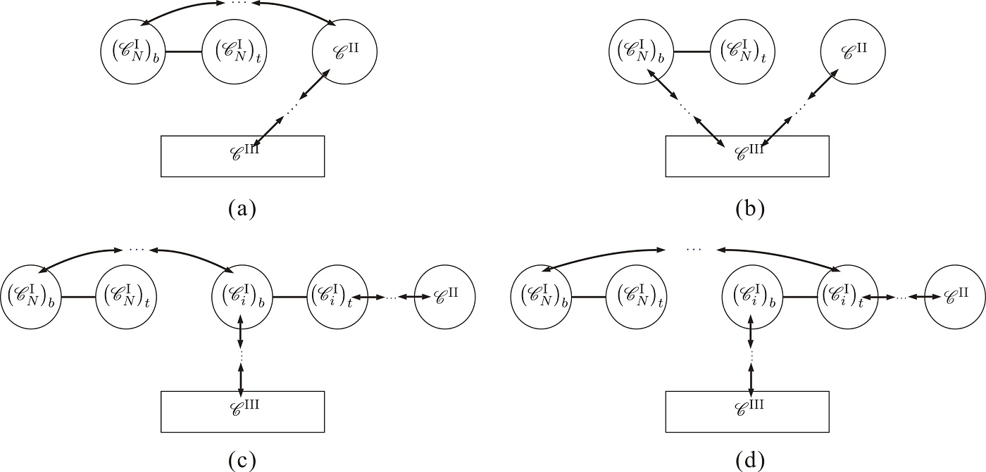
Figure 19: According to rule-1, the chain starts at the component $\mathscr{C}_{N}^{\text{I}}$ must ends at (i) the starting component (graph (a)), (ii) the ending component (graph (b)) or (iii) an internal component (graph (c) and (d)) of the chain led by $\mathscr{C}^{\text{II}}$. According to rule-2, the chain led by $\mathscr{C}_{N}^{\text{I}}$ in graphs (a)-(d) must be of the form (i) $\mathscr{U}^{\prime}=\bigl{[}\bigl{(}\mathscr{C}_{N}^{\text{I}}\bigr{)}_{t}-\bigl{(}\mathscr{C}_{N}^{\text{I}}\bigr{)}_{b},\dots,\mathscr{U}=\mathscr{C}^{\text{II}}\bigr{]}$ (graph (a)), (ii) $\mathscr{L}^{\prime}=\bigl{[}\bigl{(}\mathscr{C}_{N}^{\text{I}}\bigr{)}_{t}-\bigl{(}\mathscr{C}_{N}^{\text{I}}\bigr{)}_{b},\dots,\mathscr{L}=\mathscr{C}^{\text{III}}\bigr{]}$ (graph (b)), (iii) $\mathscr{U}^{\prime}=\bigl{[}\bigl{(}\mathscr{C}_{N}^{\text{I}}\bigr{)}_{t}-\bigl{(}\mathscr{C}_{N}^{\text{I}}\bigr{)}_{b},\dots,\mathscr{U}=\mathscr{C}^{\text{II}}\bigr{]}$ (graph (c)) and (iv) $\mathscr{L}^{\prime}=\bigl{[}\bigl{(}\mathscr{C}_{N}^{\text{I}}\bigr{)}_{t}-\bigl{(}\mathscr{C}_{N}^{\text{I}}\bigr{)}_{b},\dots,\bigl{(}\mathscr{C}_{i}^{\text{I}}\bigr{)}_{t}-\bigl{(}\mathscr{C}_{i}^{\text{I}}\bigr{)}_{b},\dots,\mathscr{L}=\mathscr{C}^{\text{III}}\bigr{]}$ (graph (d)).

All graphs $\mathcal{F}$ (all possible configurations of the final upper and lower blocks $\mathscr{U}$ and $\mathscr{L}$ as well as all possible connections of these two blocks by a type-3 line for a given configuration of $\mathscr{U}$ and $\mathscr{L}$) constructed in the above steps together form the set of physical graphs containing the skeleton $\mathcal{F}\,^{\prime}$.

The equivalence between rule-1 and -2

Rule-1 naturally inherits the chain structures of the refined graphic rule. More specifically, the chains of components are constructed by keeping track of the chains led by the highest-weight nodes in them, as we have stated in the example. In the following, we prove that there exists a one-to-one correspondence between physical graphs constructed by rule-1 and rule-2.

Any physical graph constructed by rule-1 can be understood as follows. Define the upper block by $\mathscr{U}=\mathscr{C}^{\text{II}}$, the lower block by $\mathscr{L}=\mathscr{C}^{\text{III}}$ and the reference order $\mathsf{R}^{\,\text{I}}_{\mathscr{C}}\equiv\mathsf{R}_{\mathscr{C}}\setminus\mathscr{C}^{\text{II}}=\{\mathscr{C}_{1}^{\text{I}},\mathscr{C}_{2}^{\text{I}},\dots,\mathscr{C}_{N}^{\text{I}}\}$. For a given physical graph, we find out the chain led by the highest-weight type-I component $\mathscr{C}_{N}^{\text{I}}$ in the reference order $\mathsf{R}^{\,\text{I}}_{\mathscr{C}}$. According to rule-1, this chain can be ended at any component on the chain led by the type-II component $\mathscr{C}^{\text{II}}$ because the weight of $\mathscr{C}^{\text{II}}$ is higher than $\mathscr{C}_{N}^{\text{I}}$. Since the chain that is led by $\mathscr{C}^{\text{II}}$ starts from $\mathscr{C}^{\text{II}}$, ends at $\mathscr{C}^{\text{III}}$ and can also have possible internal type-I components, the ending component of the chain led by $\mathscr{C}_{N}^{\text{I}}$ could be (i) $\mathscr{U}=\mathscr{C}^{\text{II}}$ (Fig. 19 (a)), (ii) $\mathscr{L}=\mathscr{C}^{\text{III}}$ (Fig. 19 (b)) or (iii) any internal type-I component of the chain led by $\mathscr{C}^{\text{II}}$ (Fig. 19 (c) and (d)). For the case (i), we redefine the upper block by the chain $\mathscr{U}\to\mathscr{U}^{\prime}=\bigl{[}\bigl{(}\mathscr{C}_{N}^{\text{I}}\bigr{)}_{t}-\bigl{(}\mathscr{C}_{N}^{\text{I}}\bigr{)}_{b},\dots,\mathscr{U}=\mathscr{C}^{\text{II}}\bigr{]}$ that starts at $\mathscr{C}_{N}^{\text{I}}$ and ends at the upper block $\mathscr{U}=\mathscr{C}^{\text{II}}$. For the case (ii), we redefine the lower block by the chain $\mathscr{L}\to\mathscr{L}^{\prime}=\bigl{[}\bigl{(}\mathscr{C}_{N}^{\text{I}}\bigr{)}_{t}-\bigl{(}\mathscr{C}_{N}^{\text{I}}\bigr{)}_{b},\dots,\mathscr{L}=\mathscr{C}^{\text{III}}\bigr{]}$ that starts from $\mathscr{C}_{N}^{\text{I}}$ and ends at the lower block $\mathscr{L}=\mathscr{C}^{\text{III}}$. For the case (iii), if the chain led by $\mathscr{C}_{N}^{\text{I}}$ (defined by rule-1) has the form $\bigl{[}\bigl{(}\mathscr{C}_{N}^{\text{I}}\bigr{)}_{t}-\bigl{(}\mathscr{C}_{N}^{\text{I}}\bigr{)}_{b},\dots,\bigl{(}\mathscr{C}_{i}^{\text{I}}\bigr{)}_{b}-\bigl{(}\mathscr{C}_{i}^{\text{I}}\bigr{)}_{t}\bigr{]}$ (see Fig. 19 (c)) i.e. this chain ends at the bottom side $\bigl{(}\mathscr{C}_{i}^{\text{I}}\bigr{)}_{b}$ of a component belonging to the chain led by $\mathscr{C}^{\text{II}}$, we redefine the upper block by the chain (defined by rule-2) $\mathscr{U}\to\mathscr{U}^{\prime}=\bigl{[}\bigl{(}\mathscr{C}_{N}^{\text{I}}\bigr{)}_{t}-\bigl{(}\mathscr{C}_{N}^{\text{I}}\bigr{)}_{b},\dots,\bigl{(}\mathscr{C}_{i}^{\text{I}}\bigr{)}_{b}-\bigl{(}\mathscr{C}_{i}^{\text{I}}\bigr{)}_{t},\dots,\mathscr{U}=\mathscr{C}^{\text{II}}\bigr{]}$. Else, if the chain led by $\mathscr{C}_{N}^{\text{I}}$ has the form $\bigl{[}\bigl{(}\mathscr{C}_{N}^{\text{I}}\bigr{)}_{t}-\bigl{(}\mathscr{C}_{N}^{\text{I}}\bigr{)}_{b},\dots,\bigl{(}\mathscr{C}_{i}^{\text{I}}\bigr{)}_{t}-\bigl{(}\mathscr{C}_{i}^{\text{I}}\bigr{)}_{b}\bigr{]}$, we redefine the lower block by the chain (defined by rule-2) $\mathscr{L}\to\mathscr{L}^{\prime}=\bigl{[}\bigl{(}\mathscr{C}_{N}^{\text{I}}\bigr{)}_{t}-\bigl{(}\mathscr{C}_{N}^{\text{I}}\bigr{)}_{b},\dots,\bigl{(}\mathscr{C}_{i}^{\text{I}}\bigr{)}_{t}-\bigl{(}\mathscr{C}_{i}^{\text{I}}\bigr{)}_{b},\dots,\mathscr{L}=\mathscr{C}^{\text{III}}\bigr{]}$. After finding out the chain led by $\mathscr{C}_{N}^{\text{I}}$ defined by rule-2, we remove the starting and internal components of this chain from $\mathsf{R}^{\,\text{I}}_{\mathscr{C}}\equiv\mathsf{R}_{\mathscr{C}}\setminus\mathscr{C}^{\text{II}}=\{\mathscr{C}_{1}^{\text{I}},\mathscr{C}_{2}^{\text{I}},\dots,\mathscr{C}_{N}^{\text{I}}\}$.

We find out the chain that is led by the highest-weight component in the redefined $\mathsf{R}^{\,\text{I}}_{\mathscr{C}}$ by following the previous step but using the redefined $\mathsf{R}^{\,\text{I}}_{\mathscr{C}}$, $\mathscr{U}$ and $\mathscr{L}$. Repeating these steps until the ordered set $\mathsf{R}^{\,\text{I}}_{\mathscr{C}}$ becomes empty, we get graphs with only two disjoint maximally connected subgraphs: the final upper and lower blocks. Then the graph is given by connecting the final upper and lower blocks $\mathscr{U}$ and $\mathscr{L}$ via a type-3 line. This description of the physical graphs obtained by rule-1 precisely agrees with the rule-2.

Conversely, any graph constructed according to rule-2 can also be obtained by rule-1. We define reference order $\mathsf{R}_{\mathscr{C}}\equiv\{\mathscr{C}_{1}^{\text{I}},\mathscr{C}_{2}^{\text{I}},\dots,\mathscr{C}_{N}^{\text{I}},\mathscr{C}^{\text{II}}\}$. One can always find out a path from the highest-weight component $\mathscr{C}^{\text{II}}$ in $\mathsf{R}_{\mathscr{C}}$ to $\mathscr{C}^{\text{III}}$. This path can be considered as the chain (defined by rule-1) $\bigl{[}\mathscr{C}^{\text{II}},\dots,\mathscr{C}^{\text{III}}\bigr{]}$ which starts at $\mathscr{C}^{\text{II}}$ and ends at $\mathscr{C}^{\text{III}}$. Redefine the ordered set $\mathsf{R}_{\mathscr{C}}$ by deleting the starting and internal components of this chain.

In the same way, we find out the chain (defined by rule-1) led by the highest-weight component of the reference order $\mathsf{R}_{\mathscr{C}}$ that is defined in the previous step and redefine $\mathsf{R}_{\mathscr{C}}$ again. Repeat these steps until $\mathsf{R}_{\mathscr{C}}$ becomes an empty set. Then we find that a graph constructed by rule-2 can also be obtained by rule-1.

5.3 The construction of spurious graphs

In the last example in section 4.3, we have introduced spurious graphs (see Fig. 13 (c), (f)) which are helpful when studying the relationship between the gauge invariance induced identity and BCJ relation. In general, spurious graphs are introduced for skeletons with at least three components. To see this point, we recall rule-2 for the construction of physical graphs. In the last step of rule-2, we connect the final upper and lower blocks $\mathscr{U}$ and $\mathscr{L}$ via a type-3 line by avoiding structures Fig. 17 (a) and (b) because the highest-weight chain that starts from $\mathscr{C}^{\text{II}}$ and ends at $\mathscr{C}^{\text{III}}$ must pass through kernels of all type-I components on it. Thus the chain of components led by $\mathscr{C}^{\text{II}}$ in a physical graph only contains structures of the form Fig. 17 (c) and (d). Spurious graphs are introduced as graphs where the path starting from the highest-weight node $h_{\rho(s)}$ towards a root passes through singles-sides of some components (i.e. structures Fig. 17 (a) and/or (b) existing on this path) when connecting the final upper and lower blocks via a type-3 line. A spurious graph must be associated with a proper sign. We will see soon, the spurious graphs for any given configuration of the final upper and lower blocks do not vanish. Nevertheless, we find that spurious graphs for distinct configurations of the final upper and lower blocks precisely cancel out in pairs (for example Fig. 13 (c), (f)). Therefore, the sum over all physical graphs corresponding to a given skeleton $\mathcal{F}^{\prime}$ equals to the sum over (i) all possible configurations of the final upper and lower blocks $\mathscr{U}$ and $\mathscr{L}$ for $\mathcal{F}^{\prime}$, (ii) all possible (spurious and physical) graphs which are obtained by connecting arbitrary two nodes in the final upper and lower blocks respectively by a type-3 line for a given configuration of $\mathscr{U}$ and $\mathscr{L}$. In the following, we first take the spurious graphs for the skeleton Fig. 16 as an example, then provide a general discussion on spurious graphs.

5.3.1 An example: spurious graphs for the skeleton Fig. 16

All spurious graphs for Fig. 16 are presented by Fig. 32 (a2)-(d2), Fig. 33 (a2)-(d2) and Fig. 34 (a2)-(d2). In each graph, the final upper and lower blocks are given by the two maximally connected subgraphs that contains only solid lines. We take Fig. 32 (a2) for instance. The final upper and lower blocks in in Fig. 32 (a2) are correspondingly given by $\mathscr{C}$ and the connected subgraph that is constructed by connecting both $\mathscr{A}$ and $\mathscr{B}$ with $\mathscr{R}$ by type-3 lines. When we further connect two nodes respectively belonging to $\mathscr{C}$ (the final upper block) and $\mathscr{A}_{b}$ or $\mathscr{B}_{b}$ (in the final lower block) via a type-3 line (the dashed arrow lines), spurious graph, where the path starts from $h_{\rho(s)}$ passes through a single side $\mathscr{A}_{b}$ (Fig. 32 (a2) with the line $1+$) or $\mathscr{B}_{b}$ (Fig. 32 (a2) with the line $2+$) and ends at a root, is obtained. The spurious graphs Fig. 32 (a2) together with the physical graphs Fig. 32 (a1) provide all possible graphs produced by connecting the final upper and lower blocks via a type-3 line.

An interesting observation is that each structure of spurious graph in Fig. 32 (a2)-(d2), Fig. 33 (a2)-(d2) and Fig. 34 (a2)-(d2) always appears twice. Thus we can dress the two graphs with the same structure opposite signs so that all spurious graphs cancel out in pairs after summation. As an example, the graph Fig. 32 (a2) with ‘$1+$’ line (the sign is $+$) and the graph Fig. 32.(d2) with ‘$1-$’ line (the sign is $-$) have the same structure but opposite signs.

General construction for spurious graphs with strictly defined signs is provided in the coming discussion.

5.3.2 General rule for the construction of spurious graphs

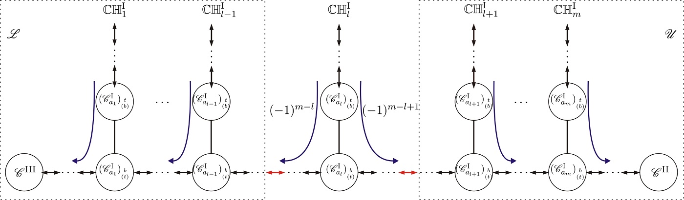
Figure 20: A typical spurious graph. There are $m$ spurious structures $\mathscr{C}_{a_{2}}^{\text{I}}$, …, $\mathscr{C}_{a_{m}}^{\text{I}}$ on the path from the highest weight node $h_{\rho(s)}$ towards a root. The chains $\mathbb{CH}_{1}^{\text{I}}$, $\mathbb{CH}_{2}^{\text{I}}$, …, $\mathbb{CH}_{l-1}^{\text{I}}$ ($\mathbb{CH}_{l+1}^{\text{I}}$, $\mathbb{CH}_{l+2}^{\text{I}}$, …, $\mathbb{CH}_{m}^{\text{I}}$) containing $\mathscr{C}_{a_{1}}^{\text{I}}$, $\mathscr{C}_{a_{2}}^{\text{I}}$, …, $\mathscr{C}_{a_{l-1}}^{\text{I}}$ ($\mathscr{C}_{a_{l+1}}^{\text{I}}$, $\mathscr{C}_{a_{l+2}}^{\text{I}}$, …, $\mathscr{C}_{a_{m}}^{\text{I}}$) must belong to the final lower (upper) block. The lowest-weight chain $\mathbb{CH}_{l}^{\text{I}}$ among $\mathbb{CH}_{i}^{\text{I}}$ $(i=1,\dots,m)$ can belong to either the final upper block (with sign $(-1)^{m-l+1}$) or the final lower one (with a sign $(-1)^{m-l}$). Thus two spurious graphs with the same configuration but opposite signs are obtained from two distinct configurations of the final upper and lower blocks, respectively.

In general, when we connect the final upper and lower blocks into a connected graph by a type-3 line, we can find the unique path starting from the highest-weight node $h_{\rho(s)}\in\mathscr{C}^{\text{II}}$ and ending at a root in $\{1,\dots,r-1\}$ (thus in $\mathscr{C}^{\text{III}}$). If there exist $m$ ($m\geq 1$) type-I components $\mathscr{C}_{a_{1}}^{\text{I}}$, $\mathscr{C}_{a_{2}}^{\text{I}}$, …, $\mathscr{C}_{a_{m}}^{\text{I}}$ such that only a single side of each is on the path, as shown by Fig. 17 (a), (b), the graph must be a spurious one. Each component $\mathscr{C}_{a_{i}}^{\text{I}}$ in a spurious graph is called a spurious component. The sign associated to the spurious graph is defined by $(-1)^{\mathcal{S}(\mathscr{U})}$, where $\mathcal{S}(\mathscr{U})$ is the number of spurious components in the final upper block. For example, in Fig. 33 (c2), $\mathcal{S}(\mathscr{U})=1,2,1$ for the graphs with lines $5-$, $12+$, $15-$ correspondingly.

To show that spurious graphs for distinct configurations always cancel in pairs, we assume that the path from $h_{\rho(s)}\in\mathscr{C}^{\text{II}}$ towards a root passes through spurious components $\mathscr{C}_{a_{i}}^{\text{I}}$ ($i=1,\dots,m$) in the order $\mathscr{C}_{a_{m}}^{\text{I}}$, …, $\mathscr{C}_{a_{2}}^{\text{I}}$, $\mathscr{C}_{a_{1}}^{\text{I}}$ for convenience. The chains (defined by rule-2) containing components $\mathscr{C}_{a_{1}}^{\text{I}}$, $\mathscr{C}_{a_{2}}^{\text{I}}$, …, $\mathscr{C}_{a_{m}}^{\text{I}}$ are correspondingly denoted by $\mathbb{CH}_{1}^{\text{I}}$, $\mathbb{CH}_{2}^{\text{I}}$, …, $\mathbb{CH}_{m}^{\text{I}}$ and their weights are denoted by $\mathcal{W}_{1}^{\text{I}}$, $\mathcal{W}_{2}^{\text{I}}$, …, $\mathcal{W}_{m}^{\text{I}}$. The lowest-weight chain among $\mathbb{CH}_{1}^{\text{I}}$, $\mathbb{CH}_{2}^{\text{I}}$, …, $\mathbb{CH}_{m}^{\text{I}}$ is assumed to be $\mathbb{CH}_{l}^{\text{I}}$. We find that the following properties of chains $\mathbb{CH}_{1}^{\text{I}}$, $\mathbb{CH}_{2}^{\text{I}}$, …, $\mathbb{CH}_{m}^{\text{I}}$ in a given spurious graph must be satisfied:

• The weights of chains $\mathcal{W}_{1}^{\text{I}}$, $\mathcal{W}_{2}^{\text{I}}$, …, $\mathcal{W}_{m}^{\text{I}}$ must satisfy

  $$\mathcal{W}_{1}^{\text{I}}>\mathcal{W}_{2}^{\text{I}}>\dots>\mathcal{W}_{l-1}^{\text{I}}>\mathcal{W}_{l}^{\text{I}},~{}~{}\mathcal{W}_{l}^{\text{I}}<\mathcal{W}_{l+1}^{\text{I}}<\dots<\mathcal{W}_{m-1}^{\text{I}}<\mathcal{W}_{m}^{\text{I}}.$$ (5.17)

  This is a consequent result of the rule-2: we always connect chains, in the descending order of their weights, to either the upper or the lower block.

• The chains $\mathbb{CH}_{1}^{\text{I}}$, $\mathbb{CH}_{2}^{\text{I}}$, …, $\mathbb{CH}_{l-1}^{\text{I}}$ ($\mathbb{CH}_{l+1}^{\text{I}}$, $\mathbb{CH}_{l+2}^{\text{I}}$, …, $\mathbb{CH}_{m}^{\text{I}}$) and structures attached to them belong to the final lower (upper) block (see Fig. 20). If not, for example the chain $\mathbb{CH}_{i}^{\text{I}}$ for given $i<l$ belongs to the final upper block, there must be at least one component (i.e. $\mathscr{C}_{a_{l}}^{\text{I}}$) with only a single side on $\mathbb{CH}_{i}^{\text{I}}$ before connecting the upper and lower blocks together. This conflicts with the definition of chains in rule-2.

According to rule-2, the lowest-weight chain $\mathbb{CH}_{l}^{\text{I}}$ (and structure attached to it) among $\mathbb{CH}_{1}^{\text{I}}$, $\mathbb{CH}_{2}^{\text{I}}$, …, $\mathbb{CH}_{m}^{\text{I}}$ can be considered to be connected with either the upper or the lower block, which have been defined previously, via a type-3 line (see Fig. 20). Thus the chain $\mathbb{CH}_{l}^{\text{I}}$ (and structure attached to it) in a given spurious graph can belong to either the final upper block or the final lower block. Correspondingly, the extra signs for these two spurious graphs, which have the same structure and distinct configurations of the final upper and lower blocks, are $(-1)^{m-l+1}$ and $(-1)^{m-l}$. As a result, all spurious graphs must cancel out in pairs.

5.4 The sum over all physical and spurious graphs

Now we are ready for rearranging the expression in the square brackets of eq. (3.5) in an appropriate form for studying the relationship between the gauge invariance induced identity eq. (2.9) and BCJ relations. For any skeleton $\mathcal{F}\,^{\prime}$, the expression in the brackets is given by

$$I=\sum\limits_{\begin{subarray}{c}\mathcal{F}\text{~{}s.t.}\\ \mathcal{F}\supset\mathcal{F}^{\prime}\end{subarray}}\mathcal{K}^{[{\mathcal{F}\setminus\mathcal{F}^{\prime}}]}\sum\limits_{\boldsymbol{\sigma}^{\mathcal{F}}}\,A(1,\boldsymbol{\sigma}^{\mathcal{F}},r).$$ (5.18)

The sum over all (physical) graphs $\mathcal{F}$ containing the skeleton $\mathcal{F}^{\prime}$ can be achieved by the following two summations.

• Sum over all possible configurations $\mathscr{U}\oplus\mathscr{L}$ of the final upper and lower blocks $\mathscr{U}$ and $\mathscr{L}$ constructed by rule-2 , including (1) all possible configurations of $\mathscr{U}$ and $\mathscr{L}$ constructed by chains of components when neglecting the inner structures of all type-II, type-III components and both sides of type-I components; (2) all possible choices of end nodes of the type-3 lines for each configuration in (1). The kinematic factor $\mathcal{K}^{\left[\mathscr{U}\oplus\mathscr{L}\setminus\mathcal{F}^{\prime}\right]}$ with respect to a given configuration $\mathscr{U}\oplus\mathscr{L}$ is the product of $k\cdot k$ factors corresponding to the type-3 lines in the final upper and lower blocks $\mathscr{U}$, $\mathscr{L}$.

• For a given configuration $\mathscr{U}\oplus\mathscr{L}$ in the previous summation, sum over all physical graphs $\mathcal{F}\in\text{Phy}\left(\mathscr{U},\mathscr{L}\right)$ which are obtained by connecting two nodes in distinct blocks via a type-3 line such that the chain led by $h_{\rho(s)}$ does not invlove structures Fig. 17 (a) and (b). The kinematic factor provided in this step is the $k\cdot k$ factor for the type-3 line between the two blocks and is denoted by $\mathcal{K}^{\left[\mathcal{F}\setminus\mathscr{U}\oplus\mathscr{L}\right]}$.

Thus $I$ is given by

$$I=\sum\limits_{\mathscr{U}\oplus\mathscr{L}}\mathcal{K}^{\left[\mathscr{U}\oplus\mathscr{L}\setminus\mathcal{F}^{\prime}\right]}\Biggl{[}\sum\limits_{\mathcal{F}\in\text{Phy}\left(\mathscr{U},\mathscr{L}\right)}\mathcal{K}^{\left[\mathcal{F}\setminus\mathscr{U}\oplus\mathscr{L}\right]}\sum\limits_{\boldsymbol{\sigma}^{\mathcal{F}}}\,A(1,\boldsymbol{\sigma}^{\mathcal{F}},r)\Biggr{]}.$$ (5.19)

Since all spurious graphs for distinct configurations of $\mathscr{U}\oplus\mathscr{L}$ corresponding to the same skeleton $\mathcal{F}^{\prime}$ must cancel out in pairs, the summation over all physical graphs for a given $\mathscr{U}\oplus\mathscr{L}$ can be extended to a summation over all physical and spurious graphs $\mathcal{F}\in\text{Phy}\left(\mathscr{U},\mathscr{L}\right)\cup\text{Spu}\left(\mathscr{U},\mathscr{L}\right)$ for a given $\mathscr{U}\oplus\mathscr{L}$. Hence we arrive

$$I=\sum\limits_{\mathscr{U}\oplus\mathscr{L}}\mathcal{K}^{\left[\mathscr{U}\oplus\mathscr{L}\setminus\mathcal{F}^{\prime}\right]}\Biggl{[}\sum\limits_{{\begin{subarray}{c}\mathcal{F}\in\text{Phy}\left(\mathscr{U},\mathscr{L}\right)\\ ~{}~{}\cup\text{Spu}\left(\mathscr{U},\mathscr{L}\right)\end{subarray}}}\mathcal{K}^{\left[\mathcal{F}\setminus\mathscr{U}\oplus\mathscr{L}\right]}\sum\limits_{\boldsymbol{\sigma}^{\mathcal{F}}}\,A(1,\boldsymbol{\sigma}^{\mathcal{F}},r)\Biggr{]}.$$ (5.20)

According to the definition, the sum over all physical and spurious graphs is nothing but the sum over all possible graphs, each of which is constructed by connecting two arbitrary nodes belonging to the final upper and lower blocks respectively via a type-3 line:

$$I=\sum\limits_{\mathscr{U}\oplus\mathscr{L}}\mathcal{K}^{\left[\mathscr{U}\oplus\mathscr{L}\setminus\mathcal{F}^{\prime}\right]}I\left[\mathscr{U},\mathscr{L}\right].$$ (5.21)

The $I\left[\mathscr{U},\mathscr{L}\right]$ for a given configuration $\mathscr{U}\oplus\mathscr{L}$ in the above equation is defined by

$$I\left[\mathscr{U},\mathscr{L}\right]\equiv\sum\limits_{\mathcal{F}\in\left(\mathscr{U},\mathscr{L}\right)}(-)^{\mathcal{F}}\mathcal{K}^{\left[\mathcal{F}\setminus\mathscr{U}\oplus\mathscr{L}\right]}\sum\limits_{\boldsymbol{\sigma}^{\mathcal{F}}}\,A(1,\boldsymbol{\sigma}^{\mathcal{F}},r),$$ (5.22)

where

$$(-)^{\mathcal{F}}=(-1)^{\mathcal{N}(\mathscr{U})+\mathcal{N}(\mathscr{L})+\mathcal{S}(\mathscr{U})+1}$$ (5.23)

is a proper sign depending on the total number of arrows pointing deviate from the direction of root ($\mathcal{N}(\mathscr{U})$ for the final upper block, $\mathscr{N}(\mathscr{L})$ for the final lower block and $1$ for the type-3 line between the two blocks) and the number $\mathcal{S}(\mathscr{U})$ of spurious components in the final upper block of a graph.

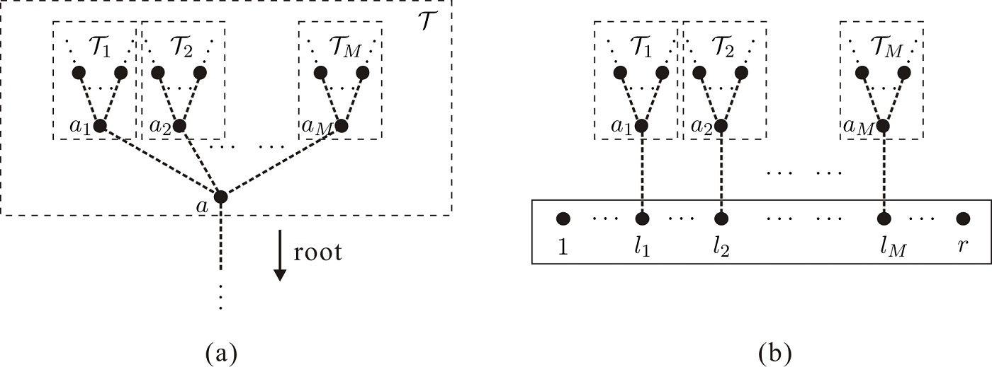
Figure 21: (a): A typical tree structure with sub-trees planted at the node $a$, (b): A typical graph with trees planted at roots $l_{1},\dots,l_{M}\in\{1,\dots,r-1\}$.

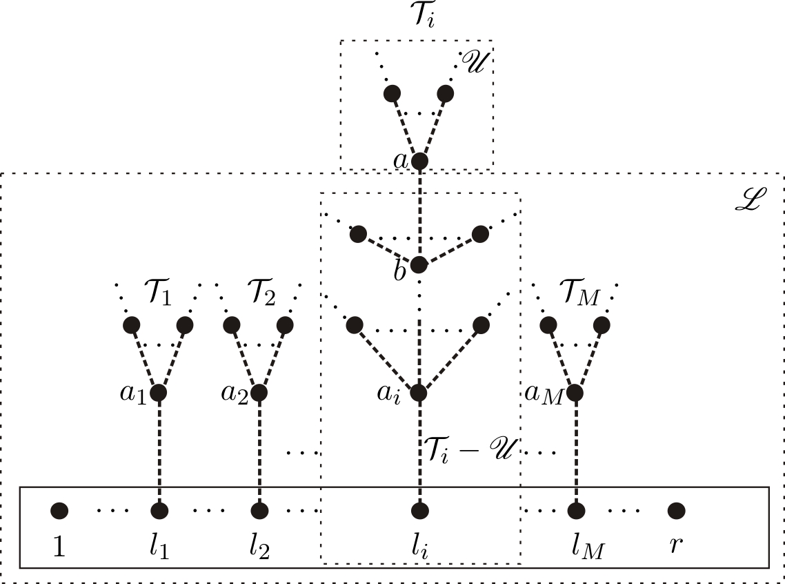
Figure 22: Permutations established by a graph with trees $\mathcal{T}_{1},\mathcal{T}_{2},\dots,\mathcal{T}_{M}$ planted at roots $l_{1},l_{2},\dots,l_{M}\in\{1,\dots,r-1\}$ are given by eq. (5.26). The nearest-to-root nodes in these trees are correspondingly $a_{1},a_{2},\dots,a_{M}$. The final upper block belongs to the tree $\mathcal{T}_{i}$ which is rooted at $l_{i}\in\{1,\dots,r-1\}$. Nodes $b\in\mathscr{L}$ and $a\in\mathscr{U}$ are the two nodes that belong to distinct blocks and connected by a type-3 line. According to whether the nodes belong to the final upper or lower block, the tree $\mathcal{T}_{i}$ is divided into two parts $\mathscr{U}$ and $\mathcal{T}_{i}-\mathscr{U}$.

Comments on the expression eq. (5.22)

Permutations $\bf\boldsymbol{\sigma}^{\mathcal{F}}$   From the graphic rule, we can see permutations $\bf\boldsymbol{\sigma}^{\mathcal{F}}$ for a given graph $\mathcal{F}\in\left(\mathscr{U},\mathscr{L}\right)$ do not rely on types of lines. They only depend on the relative positions between nodes in a graph. Therefore, in the following we replace all types of lines in $\mathcal{F}$ by dashed lines with no arrow when considering permutations $\boldsymbol{\sigma}^{\mathcal{F}}$ established by a graph ${\mathcal{F}}$. For each graph $\mathcal{F}$, the possible permutations $\boldsymbol{\sigma}^{\mathcal{F}}$ are collected as follows:

• The relative order of roots is always $(\sigma^{\mathcal{F}})^{-1}(1)<(\sigma^{\mathcal{F}})^{-1}(2)<\dots<(\sigma^{\mathcal{F}})^{-1}(r-1)$. We set $\sigma^{-1}(r)=\infty$ to require that the element $r$ is always the last one in the permutation $\boldsymbol{\sigma}^{\mathcal{F}}$.

• For tree structures planted at roots $\{1,2,\dots,r-1\}$, if two elements $a,b\in\mathsf{H}$ are on a same path which starts from an element of $\mathsf{H}$ and end at an arbitrary root $l\in\{1,2,\dots,r-1\}$ and satisfy the condition that $a$ is nearer to the root $l$ than $b$, we have $(\sigma^{\mathcal{F}})^{-1}(l)<(\sigma^{\mathcal{F}})^{-1}(a)<(\sigma^{\mathcal{F}})^{-1}(b)$.

• If a node $a\in\mathsf{H}$ in a connected tree structure $\mathcal{T}$ (shown by Fig. 21 (a)) is nearer to root than all other nodes in $\mathcal{T}$ and $a$ is attached by $M$ connected sub-tree structures (branches) $\mathcal{T}_{1}$, $\mathcal{T}_{2}$,…,$\mathcal{T}_{M}$ ($M\geq 2$) (where the nodes nearest to $a$ in these branches are $a_{1}$, $a_{2}$,…,$a_{M}$ correspondingly), the collection of all possible relative orders for nodes in $\mathcal{T}$ are recursively expressed by

  $${\mathcal{T}}\big{|}_{a}=\bigl{\{}a,{\mathcal{T}_{1}}\big{|}_{a_{1}}\shuffle{\mathcal{T}_{2}}\big{|}_{a_{2}}\shuffle\dots\shuffle{\mathcal{T}_{M}}\big{|}_{a_{M}}\bigr{\}},$$ (5.24)

  where $\mathcal{T}\big{|}_{a}$ denotes all possible permutations established by $\mathcal{T}$ with the leftmost element $a$.

• Suppose there are $M$ connected tree structures $\mathcal{T}_{1}$, $\mathcal{T}_{2}$,…,$\mathcal{T}_{M}$ planted at roots $l_{1},l_{2},\dots,l_{M}\in\{1,\dots,r-1\}$ in a graph $\mathcal{F}$ correspondingly while the nearest-to-roots elements with respect to these tree structures are $a_{1}$, $a_{2}$,…,$a_{M}$ (see Fig. 21 (b)). The permutations $\boldsymbol{\sigma}^{\mathcal{F}}$ of elements in $\mathsf{H}\cup\{1,\dots,r\}$ satisfy

  $$\boldsymbol{\sigma}^{\mathcal{F}}\in\bigl{\{}1,\bigl{\{}2,\dots,r-1\bigr{\}}\shuffle{\mathcal{T}_{1}}\big{|}_{a_{1}}\shuffle{\mathcal{T}_{2}}\big{|}_{a_{2}}\shuffle\dots\shuffle{\mathcal{T}_{M}}\big{|}_{a_{M}},r\bigr{\}}\Big{|}_{\begin{subarray}{c}l_{i}\prec a_{i}\\ (i=1,\dots,M)\end{subarray}},$$ (5.25)

  where $a\prec b$ in a permutation $\boldsymbol{\sigma}$ means $\sigma^{-1}(a)<\sigma^{-1}(b)$.

Rearrangement of eq. (5.22)   Since the graph $\mathcal{F}$ is given by connecting any node $a$ in the final upper block $\mathscr{U}$ and any node $b$ in the final lower block $\mathscr{L}$ via a type-3 line, the factor $\mathcal{K}^{\left[\mathcal{F}\setminus\mathscr{U}\oplus\mathscr{L}\right]}$ is just $k_{a}\cdot k_{b}$ while the sum over all $\mathcal{F}\in\left(\mathscr{U},\mathscr{L}\right)$ is given by summing over all choices of nodes $a\in\mathscr{U}$ and $b\in\mathscr{L}$. Permutations $\boldsymbol{\sigma}^{\mathcal{F}}$ can be understood as follows:

• Suppose that all tree structures planted at roots $l_{1},l_{2},\dots,l_{M}\in\{1,\dots,r-1\}$ in a given (physical or spurious) graph $\mathcal{F}$ are $\mathcal{T}_{1}$, $\mathcal{T}_{2}$, …, $\mathcal{T}_{M}$ and the nearest-to-root elements with respect to these tree structures are $a_{1}$, $a_{2}$, …, $a_{M}$ correspondingly (see Fig. 22). The final upper block $\mathscr{U}$ (connected to the node $b\in\mathscr{L}$), when all lines therein are replaced by dashed lines, must belong to some connected tree structure $\mathcal{T}_{i}$ which is attached to a root $l_{i}$. Permutations $\boldsymbol{\sigma}^{\mathcal{F}}$ then satisfy

  $$\boldsymbol{\sigma}^{\mathcal{F}}\in\Bigl{\{}1,\bigl{\{}2,\dots,r-1\bigr{\}}\shuffle{\mathcal{T}_{1}}\big{|}_{a_{1}}\shuffle\dots\shuffle\bigl{(}(\mathcal{T}_{i}-\mathscr{U})\big{|}_{a_{i}}\shuffle\mathscr{U}\big{|}_{a}\bigr{)}\big{|}_{b\prec a}\shuffle\dots\shuffle{\mathcal{T}_{M}}\big{|}_{a_{M}},r\Bigr{\}}\Big{|}_{\begin{subarray}{c}l_{i}\prec a_{i}\\ (i=1,\dots,M)\end{subarray}}.$$ (5.26)

• Any permutation $\boldsymbol{\sigma}^{\mathcal{F}}$ satisfying eq. (5.26) can be obtained by shuffling $\boldsymbol{\zeta}\in{\mathscr{U}}\big{|}_{a}$ (a relative order of elements in $\mathscr{U}$) with $\boldsymbol{\gamma}$ (a relative order of elements in $\mathscr{L}$)

  $$\boldsymbol{\gamma}\in\Bigl{\{}\bigl{\{}2,\dots,r-1\bigr{\}}\shuffle{\mathcal{T}_{1}}\big{|}_{a_{1}}\shuffle\dots\shuffle(\mathcal{T}_{i}-\mathscr{U})\big{|}_{a_{i}}\shuffle\dots\shuffle{\mathcal{T}_{M}}\big{|}_{a_{M}}\Big{\}}\Big{|}_{\begin{subarray}{c}l_{i}\prec a_{i}\\ (i=1,\dots,M)\end{subarray}}$$ (5.27)

  such that $({\sigma}^{\mathcal{F}})^{-1}(b)<({\sigma}^{\mathcal{F}})^{-1}(a)$. Thus all permutations $\boldsymbol{\sigma}^{\mathcal{F}}$ in eq. (5.22) satisfy $\boldsymbol{\sigma}^{\mathcal{F}}\in\big{\{}1,\boldsymbol{\gamma}\shuffle\boldsymbol{\zeta},r\big{\}}\big{|}_{({\sigma}^{\mathcal{F}})^{-1}(b)<({\sigma}^{\mathcal{F}})^{-1}(a)}$ for a given $\boldsymbol{\gamma}$ satisfying eq. (5.27) and a given $\boldsymbol{\zeta}\in{\mathscr{U}}\big{|}_{a}$.

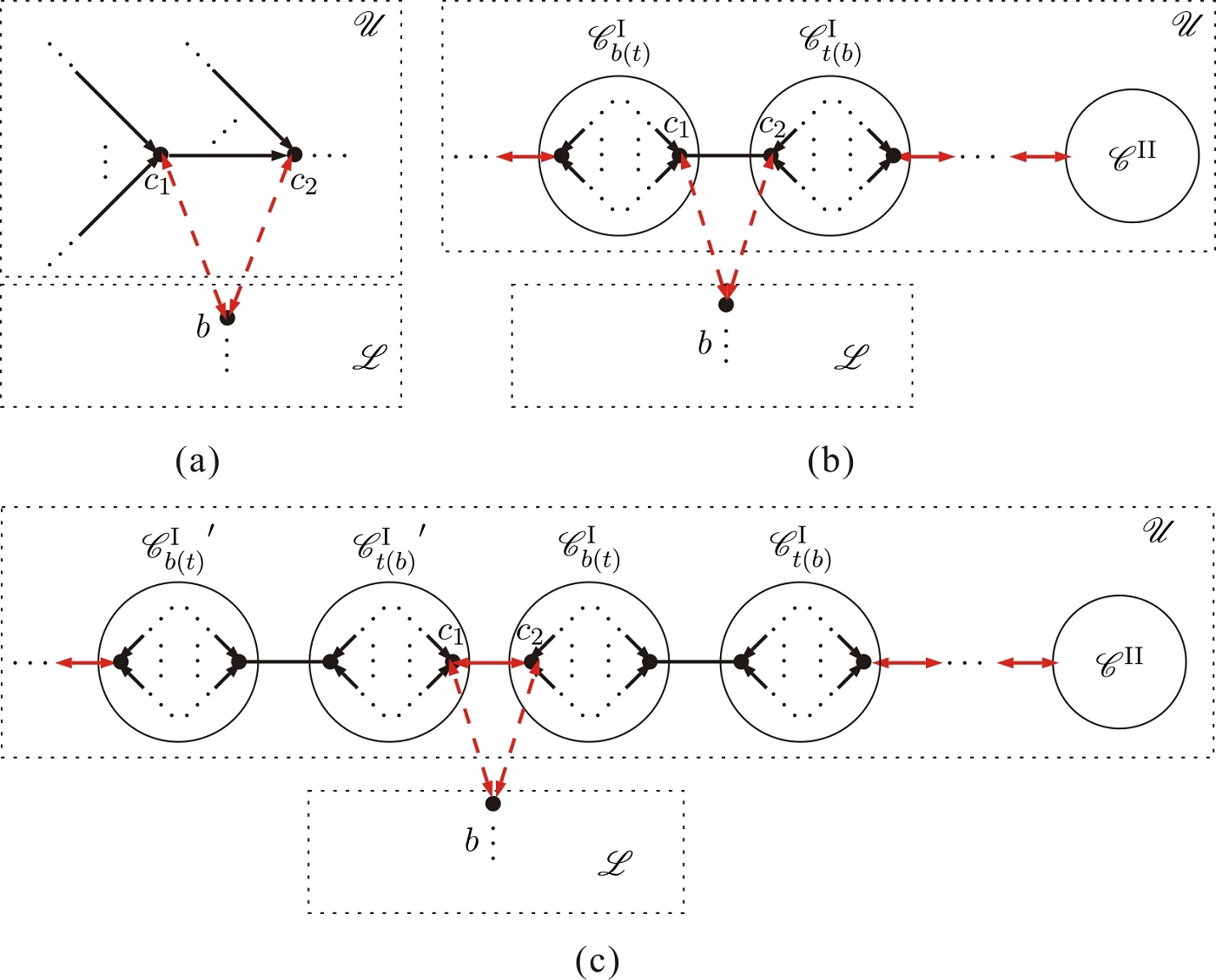
Figure 23: For any given configuration of the final upper and lower blocks $\mathscr{U}$ and $\mathscr{L}$, the factors $(-1)^{\tiny\mathcal{N}(\mathscr{L})+\mathcal{N}(\mathscr{U}_{c})+\mathcal{S}(\mathscr{U}_{c})+1}$ for graphs with $a=c_{1}$ and $a=c_{2}$ ($c_{1}$, $c_{2}$ are two adjacent nodes in the final upper block) always have opposite signs. Particularly, the number $\mathcal{N}(\mathscr{L})$ is always independent of the choice of $a$. When we consider the number $\mathcal{N}(\mathscr{U}_{c})+\mathcal{S}(\mathscr{U}_{c})$, there are three possible cases: (i) In (a), $c_{1}$ and $c_{2}$ are two end nodes of a type-3 line and they both belong to a same top or bottom side of some type-I component. The two graphs corresponding to $a=c_{1}$ and $a=c_{2}$ must have the same $\mathcal{S}(\mathscr{U}_{c})$, but $\mathcal{N}(\mathscr{U}_{c_{1}})=\mathcal{N}(\mathscr{U}_{c_{2}})+1$. (ii) In (b), $c_{1}$ and $c_{2}$ are two end nodes of a type-1 line. Since a type-1 line does node carry arrow, we have $\mathcal{N}(\mathscr{U}_{c_{1}})=\mathcal{N}(\mathscr{U}_{c_{2}})$. The component $\mathscr{C}^{\text{I}}$ is a spurious one for the graph with $a=c_{2}$ but not spurious for the graph with $a=c_{1}$, thus $\mathcal{S}(\mathscr{U}_{c_{1}})=\mathcal{S}(\mathscr{U}_{c_{2}})-1$. (iii) Similarly, in (c), where $c_{1}$ and $c_{2}$ are two end nodes of a type-3 line, we have $\mathcal{N}(\mathscr{U}_{c_{1}})=\mathcal{N}(\mathscr{U}_{c_{2}})$ and $\mathcal{S}(\mathscr{U}_{c_{1}})=\mathcal{S}(\mathscr{U}_{c_{2}})+1$.

Having the above observations in hand, we reexpress eq. (5.22) by

$$I\left[\mathscr{U},\mathscr{L}\right]~{}~{}~{}~{}$$

$$= \sum\limits_{a\in\mathscr{U}}\sum\limits_{\begin{subarray}{c}b\in\mathscr{L}\\ b\neq r\end{subarray}}(-1)^{\tiny\mathcal{N}(\mathscr{L})+\mathcal{N}(\mathscr{U}_{a})+\mathcal{S}(\mathscr{U}_{a})+1}(k_{a}\cdot k_{b})\sum\limits_{\boldsymbol{\zeta}\in{\mathscr{U}}|_{a}}\sum\limits_{\boldsymbol{\gamma}}\sum\limits_{\boldsymbol{\sigma}}A\bigl{(}1,\boldsymbol{\sigma}\in(\boldsymbol{\zeta}\shuffle\boldsymbol{\gamma})\big{|}_{\tiny({\sigma})^{-1}(b)<({\sigma})^{-1}(a)},r\bigr{)},$$

where all $\boldsymbol{\gamma}$ satisfy eq. (5.27) and $\boldsymbol{\zeta}\in{\mathscr{U}}|_{a}$ are the permutation for the final upper block when considering $a$ is the nearest to root node in $\mathscr{U}$. For a given $\mathscr{U}$, $\mathcal{N}(\mathscr{U}_{a})$ and $\mathcal{S}(\mathscr{U}_{a})$ are the $\mathcal{N}(\mathscr{U})$ and $\mathcal{S}(\mathscr{U})$ for choosing a given node $a\in\mathscr{U}$. Note that $\mathcal{N}(\mathscr{L})$ is independent of the choice of $b$ in the final lower block $\mathscr{L}$. Since the choices of nodes $a$ and $b$ are independent of each other, the above expression can be further arranged as

$$I\left[\mathscr{U},\mathscr{L}\right]$$

$$= (-1)^{\tiny\mathcal{N}(\mathscr{L})}\sum\limits_{\boldsymbol{\gamma}}\biggl{\{}\sum\limits_{a\in\mathscr{U}}\sum\limits_{\boldsymbol{\zeta}\in{\mathscr{U}}|_{a}}(-1)^{\tiny\mathcal{N}(\mathscr{U}_{a})+\mathcal{S}(\mathscr{U}_{a})+1}\biggl{[}\sum\limits_{\begin{subarray}{c}b\in\mathscr{L}\\ b\neq r\end{subarray}}(k_{a}\cdot k_{b})\sum\limits_{\boldsymbol{\sigma}}A\bigl{(}1,\boldsymbol{\sigma}\in(\boldsymbol{\zeta}\shuffle\boldsymbol{\gamma})\big{|}_{\tiny({\sigma})^{-1}(b)<({\sigma})^{-1}(a)},r\bigr{)}\biggr{]}\biggr{\}}.$$

As we have shown in examples in section 4, when we collect coefficients for any given permutation $\boldsymbol{\sigma}\in\boldsymbol{\gamma}\shuffle\boldsymbol{\zeta}$ together, the expression in the square brackets in eq. (5.4) is given by

$$(k_{a}\cdot Y_{a}(\boldsymbol{\sigma}))A\bigl{(}1,\boldsymbol{\sigma}\in(\boldsymbol{\zeta}\shuffle\boldsymbol{\gamma}),r\bigr{)}.~{}~{}$$ (5.30)

Here $Y_{a}(\boldsymbol{\sigma})$ is the sum of all momenta of elements in $\boldsymbol{\gamma}$ (the element $1$ is also included) appearing on the LHS of the node $a$ in $\boldsymbol{\sigma}$. The factor $(-1)^{\tiny\mathcal{N}(\mathscr{U}_{a})+\mathcal{S}(\mathscr{U}_{a})+1}$ in eq. (5.4) depends on the choice of $a$. Once the node $a\in\mathscr{U}$ (i.e. the node nearest to root in $\mathscr{U}$) under the first summation in the braces of eq. (5.4) is fixed, both the number $\mathcal{N}(\mathscr{U}_{a})$ of arrows pointing deviate from the direction of root and the number $\mathcal{S}(\mathscr{U}_{a})$ of spurious components in $\mathscr{U}$ are fixed. To analyze the relation between signs corresponding to distinct choices of $a$, we consider two adjacent nodes $c_{1},c_{2}\in\mathscr{U}$ which can be connected via all three types of lines:

• If the line between $c_{1}$ and $c_{2}$ is a type-2 line, as shown by Fig. 23 (a), the factors for choosing $a=c_{1}$ and $a=c_{2}$ are related by flipping the sign, i.e. $(-1)^{\mathcal{N}(\mathscr{U}_{c_{1}})}=(-1)^{\mathcal{N}(\mathscr{U}_{c_{2}})\pm 1}$ because the difference of the numbers of all arrows deviating from root for these two choices is $1$.

• If $c_{1}$ and $c_{2}$ are two ends of a type-1 line or a type-3 line, as shown by Fig. 23 (b) and (c), the number of arrows that deviate from root are same for $a=c_{1}$ and $a=c_{2}$. Thus $(-1)^{\mathcal{N}(\mathscr{U}_{c_{1}})}=(-1)^{\mathcal{N}(\mathscr{U}_{c_{2}})}$. Nevertheless, we should also count the number $\mathcal{S}(\mathscr{U})$ of spurious chains in a (spurious) graph. Assume that the distance between $c_{1}$ and the (highest weight) node $h_{\rho(s)}$ is always larger than that between $c_{2}$ and $h_{\rho(s)}$. If $c_{1}$, $c_{2}$ are two end nodes of a type-1 (or type-3) line, the numbers of spurious components $\mathcal{S}(\mathscr{U})$ for these two cases always differ by $1$. Thus the factors $(-1)^{\mathcal{S}(\mathscr{U}_{a})}$ for choosing $a=c_{1}$ and $a=c_{2}$ always have the opposite sign.

To sum up, the factors $(-1)^{\tiny\mathcal{N}(\mathscr{U}_{a})+\mathcal{S}(\mathscr{U}_{a})+1}$ associated with graphs corresponding to $a=c_{1}$ and $a=c_{2}$, where $c_{1},c_{2}\in\mathcal{U}$ are two adjacent nodes connected by an arbitrary type of line, always differ by a factor $(-1)$. Replacing the expression in the square brackets of eq. (5.4) by eq. (5.30) and considering the relative signs, we rewrite eq. (5.30) as

$$I\left[\mathscr{U},\mathscr{L}\right]=(-1)^{\tiny\mathcal{N}(\mathscr{L})+\mathcal{N}(\mathscr{U}_{c})+\mathcal{S}(\mathscr{U}_{c})+1}\sum\limits_{\boldsymbol{\gamma}}\biggl{[}\sum\limits_{a\in\mathscr{U}}f^{a}\sum\limits_{\boldsymbol{\zeta}\in{\mathscr{U}}|_{a}}\sum\limits_{\boldsymbol{\sigma}}(k_{a}\cdot Y_{a}(\boldsymbol{\sigma}))A\bigl{(}1,\boldsymbol{\sigma}\in(\boldsymbol{\zeta}\shuffle\boldsymbol{\gamma}),r\bigr{)}\biggr{]},$$ (5.31)

where the factor $(-1)^{\tiny\mathcal{N}(\mathscr{L})+\mathcal{N}(\mathscr{U}_{c})+\mathcal{S}(\mathscr{U}_{c})+1}$ for a fixed $c\in\mathscr{U}$ eq. (5.4) has been exacted out. The relative signs $f^{a}$ for choosing $a$ as other nodes can be fully fixed because the factor for any two adjacent choices of $a$ must be differ by a factor $(-1)$. In the next section, we will prove that for any given $\boldsymbol{\gamma}$, the expression in the brackets of eq. (5.31) must vanish because it can always be written as a combination of BCJ relations.

6 Graph-based BCJ relation as a combination of traditional BCJ relations

In this section, we introduce the following graph-based BCJ relation

$$\sum\limits_{a\in\mathcal{T}}f^{a}\sum\limits_{\boldsymbol{\zeta}\in{\mathcal{T}}|_{a}}\sum\limits_{\boldsymbol{\sigma}}\left[k_{a}\cdot Y_{a}(\boldsymbol{\sigma})\right]\,A\left(1,\boldsymbol{\sigma}\in(\boldsymbol{\zeta}\shuffle\,\boldsymbol{\gamma}),r\right)=0.~{}~{}$$ (6.1)

Here, $\boldsymbol{\gamma}$ is an arbitrary permutation of elements in $\{2,\dots,r-1\}$ and $\mathcal{T}$ is an arbitrary connected tree graph. We use $\mathcal{T}|_{a}$ to denote the relative orders between nodes of $\mathcal{T}$ when choosing the node $a$ as the leftmost one (see section 5.4). For a given graph $\mathcal{T}$, the factor $f^{a}$ is a relative sign depending on the choice of $a$. This factor is fixed as follows: (i) Choose an arbitrary node $c$ and require $f^{c}=1$, (ii) For arbitrary two adjacent nodes $c_{1}$ and $c_{2}$, we have $f^{c_{1}}=-f^{c_{2}}$. In the following, we use $\mathcal{B}^{\,c}_{G}(1\,|\,\mathcal{T},\boldsymbol{\gamma}\,|\,r)$ to stand for the LHS of eq. (6.1) with choosing $f^{c}=1$ ($c\in\mathcal{T}$). We will prove that the $\mathcal{B}^{\,c}_{G}(1\,|\,\mathcal{T},\boldsymbol{\gamma}\,|\,r)$ (thus eq. (5.31) and eq. (5.21)) is a combination of the LHS of traditional BCJ relations eq. (2.10) (see eq. (2.11)). As a result, the gauge invariance induced identity eq. (2.9) can always be expanded in terms of traditional BCJ relations.

6.1 Examples

Now we present several examples for the graph-based BCJ relation eq. (6.1).
Example-1
The simplest example is that the tree graph $\mathcal{T}$ consists of only a single node $h_{1}$. The LHS of eq. (6.1) is nothing but the LHS of a fundamental BCJ relation

$$\mathcal{B}^{\,h_{1}}_{G}\big{(}1\big{|}\includegraphics[width=5.69046pt]{GraphBasedEG1.jpg},\boldsymbol{\gamma}\big{|}r\big{)}=\mathcal{B}(1|\{h_{1}\},\boldsymbol{\gamma}|r).$$ (6.2)

Example-2
The next simplest example is that $\mathcal{T}$ consists of two nodes $h_{1}$ and $h_{2}$ with one (dashed) line between them. The LHS of eq. (6.1) in this case reads

$$\mathcal{B}^{h_{1}}_{G}\big{(}1\big{|}\includegraphics[width=28.90755pt]{GraphBasedEG2.jpg},\boldsymbol{\gamma}\big{|}r\big{)}=\sum\limits_{\shuffle}(k_{h_{1}}\cdot Y_{h_{1}}(\shuffle))A(1,\{h_{1},h_{2}\}\shuffle\boldsymbol{\gamma},r)-\sum\limits_{\shuffle}(k_{h_{2}}\cdot Y_{h_{2}}(\shuffle))A(1,\{h_{2},h_{1}\}\shuffle\boldsymbol{\gamma},r).$$ (6.3)

Notice that the last term can be replaced by

$$\mathcal{B}^{h_{2}}_{G}\big{(}1\big{|}\includegraphics[width=5.44864pt]{GraphBasedEG3.jpg},\{h_{1}\}\shuffle\boldsymbol{\gamma}\big{|}r\big{)}-\sum\limits_{\shuffle}(k_{h_{2}}\cdot X_{h_{2}}(\shuffle))A(1,\{h_{1},h_{2}\}\shuffle\boldsymbol{\gamma},r).$$ (6.4)

The second term of the above equation together with the first term of eq. (6.3) produces the LHS of the traditional BCJ relation eq. (2.10) with $\boldsymbol{\beta}=\{h_{1},h_{2}\}$, i.e. $\mathcal{B}(1\,|\,\{h_{1},h_{2}\},\boldsymbol{\gamma}\,|\,r)$. Thus eq. (6.3) is finally given by

$$\mathcal{B}^{h_{1}}_{G}\big{(}1\big{|}\includegraphics[width=28.90755pt]{GraphBasedEG2.jpg},\boldsymbol{\gamma}\big{|}r\big{)} = \mathcal{B}(1|\{h_{1},h_{2}\},\boldsymbol{\gamma}|r)-\mathcal{B}^{h_{2}}_{G}\big{(}1\big{|}\includegraphics[width=5.44864pt]{GraphBasedEG3.jpg},\{h_{1}\}\shuffle\boldsymbol{\gamma}\big{|}r\big{)}=\mathcal{B}(1|\{h_{1},h_{2}\},\boldsymbol{\gamma}|r)-\mathcal{B}(1|\{h_{2}\},\{h_{1}\}\shuffle\boldsymbol{\gamma}|r),$$

which is a combination of the LHS of traditional BCJ relations. It is worth pointing out that the above expression is not unique. When exchanging the roles of $h_{1}$ and $h_{2}$ in eq. (6.1), we get another equivalent expansion

$$\mathcal{B}^{h_{2}}_{G}\big{(}1\big{|}\includegraphics[width=28.90755pt]{GraphBasedEG2.jpg},\boldsymbol{\gamma}\big{|}r\big{)}=\mathcal{B}(1|\{h_{2},h_{1}\},\boldsymbol{\gamma}|r)+\mathcal{B}(1|\{h_{1}\},\{h_{2}\}\shuffle\boldsymbol{\gamma}|r)=-\mathcal{B}^{h_{1}}_{G}\big{(}1\big{|}\includegraphics[width=28.90755pt]{GraphBasedEG2.jpg},\boldsymbol{\gamma}\big{|}r\big{)}.$$ (6.6)

Example-3
Now we consider a graph with three nodes $\mathcal{T}=\includegraphics[width=45.52458pt]{GraphBasedEG4.jpg}$. The LHS of eq. (6.1) for this graph reads

$$\mathcal{B}^{h_{1}}_{G}\big{(}1\big{|}\includegraphics[width=45.52458pt]{GraphBasedEG4.jpg},\boldsymbol{\gamma}\big{|}r\big{)}$$

$$= \sum\limits_{\shuffle}(k_{h_{1}}\cdot Y_{h_{1}}(\shuffle))A(1,\{h_{1},h_{2},h_{3}\}\shuffle\boldsymbol{\gamma},r)-\Bigl{[}\sum\limits_{\shuffle_{1},\shuffle_{2}}(k_{h_{2}}\cdot Y_{h_{2}}(\shuffle_{1},\shuffle_{2}))A(1,\{h_{2},\{h_{1}\}\shuffle_{1}\{h_{3}\}\}\shuffle_{2}\boldsymbol{\gamma},r)$$

$$-\sum\limits_{\shuffle}(k_{h_{3}}\cdot Y_{h_{3}}(\shuffle))A(1,\{h_{3},h_{2},h_{1}\}\shuffle\boldsymbol{\gamma},r)\Bigr{]}.$$

The expression in the square brackets can be considered as $\sum\limits_{\shuffle}\mathcal{B}^{h_{2}}_{G}\big{(}1\big{|}\includegraphics[width=28.90755pt]{GraphBasedEG5.jpg},\{h_{1}\}\shuffle\boldsymbol{\gamma}\big{|}r\big{)}\big{|}_{h_{2}\prec h_{1}}$, where $h_{2}\prec h_{1}$ for a given permutation $\boldsymbol{\xi}$ means that $\xi^{-1}(h_{2})<\xi^{-1}(h_{1})$. When the first equality of eq. (6.1) in example-2 is applied, $\sum\limits_{\shuffle}\mathcal{B}^{h_{2}}_{G}\big{(}1\big{|}\includegraphics[width=28.90755pt]{GraphBasedEG5.jpg},\{h_{1}\}\shuffle\boldsymbol{\gamma}\big{|}r\big{)}\big{|}_{h_{2}\prec h_{1}}$ turns to

$$\sum\limits_{\shuffle}\mathcal{B}^{h_{2}}_{G}\big{(}1\big{|}\includegraphics[width=28.90755pt]{GraphBasedEG5.jpg},\{h_{1}\}\shuffle\boldsymbol{\gamma}\big{|}r\big{)}\big{|}_{h_{2}\prec h_{1}}$$

$$= \sum\limits_{\shuffle}\mathcal{B}(1|\{h_{2},h_{3}\},\{h_{1}\}\shuffle\boldsymbol{\gamma}|r)|_{h_{2}\prec h_{1}}-\sum\limits_{\shuffle}\mathcal{B}^{h_{3}}_{G}\big{(}1\big{|}\includegraphics[width=5.69046pt]{GraphBasedEG9.jpg},\{h_{2},h_{1}\}\shuffle\boldsymbol{\gamma}\big{|}r\big{)}$$

$$= \sum\limits_{\shuffle}\mathcal{B}(1|\{h_{2},h_{3}\},\{h_{1}\}\shuffle\boldsymbol{\gamma}|r)-\mathcal{B}(1|\{h_{2},h_{3}\},\{h_{1}\}\shuffle\boldsymbol{\gamma}|r)|_{h_{1}\prec h_{2}}-\sum\limits_{\shuffle}\mathcal{B}^{h_{3}}_{G}\big{(}1\big{|}\includegraphics[width=5.69046pt]{GraphBasedEG9.jpg},\{h_{2},h_{1}\}\shuffle\boldsymbol{\gamma}\big{|}r\big{)}.$$

The first term and the third term on the last line are just a combination of LHS of BCJ relations with $\boldsymbol{\beta}=\{h_{2},h_{3}\}$ and $\boldsymbol{\beta}=\{h_{3}\}$ respectively. The sum of the second term on the last line of the above equation and the first term in eq. (6.1) is nothing but the LHS of traditional BCJ relation eq. (2.10) with $\boldsymbol{\beta}=\{h_{1},h_{2},h_{3}\}$. Hence eq. (6.1) is finally expanded into the following two parts

$$\mathcal{B}^{h_{1}}_{G}\big{(}1\big{|}\includegraphics[width=45.52458pt]{GraphBasedEG4.jpg},\boldsymbol{\gamma}\big{|}r\big{)}=\mathcal{B}^{{(1)}}_{G}\big{(}1\big{|}\includegraphics[width=45.52458pt]{GraphBasedEG4.jpg}\big{|}_{h_{1}},\boldsymbol{\gamma}\big{|}r\big{)}+\sum\limits_{\shuffle}\mathcal{B}^{{(2)}}_{G}\big{(}1\big{|}\includegraphics[width=28.90755pt]{GraphBasedEG5.jpg},\{h_{1}\}\shuffle\boldsymbol{\gamma}\big{|}r\big{)},$$ (6.9)

where $\mathcal{B}^{{(1)}}_{G}\big{(}1\big{|}\includegraphics[width=45.52458pt]{GraphBasedEG4.jpg}\big{|}_{h_{1}},\boldsymbol{\gamma}\big{|}r\big{)}$ and $\sum\limits_{\shuffle}\mathcal{B}^{{(2)}}_{G}\big{(}1\big{|}\includegraphics[width=28.90755pt]{GraphBasedEG5.jpg},\{h_{1}\}\shuffle\boldsymbol{\gamma}\big{|}r\big{)}$ are defined by

$$\mathcal{B}^{{(1)}}_{G}\big{(}1\big{|}\includegraphics[width=45.52458pt]{GraphBasedEG4.jpg}\big{|}_{h_{1}},\boldsymbol{\gamma}\big{|}r\big{)} \equiv \mathcal{B}(1|\{h_{1},h_{2},h_{3}\},\boldsymbol{\gamma}|r),$$

$$\sum\limits_{\shuffle}\mathcal{B}^{{(2)}}_{G}\big{(}1\big{|}\includegraphics[width=28.90755pt]{GraphBasedEG5.jpg},\{h_{1}\}\shuffle\boldsymbol{\gamma}\big{|}r\big{)} \equiv \sum\limits_{\shuffle}\big{[}-\mathcal{B}(1|\{h_{2},h_{3}\},\{h_{1}\}\shuffle\boldsymbol{\gamma}|r)+\mathcal{B}(1|\{h_{3}\},\{h_{2},h_{1}\}\shuffle\boldsymbol{\gamma}|r)\big{]}.$$ (6.10)

The expression of $\mathcal{B}^{{(1)}}_{G}\big{(}1\big{|}\includegraphics[width=45.52458pt]{GraphBasedEG4.jpg}\big{|}_{h_{1}},\boldsymbol{\gamma}\big{|}r\big{)}$ is the LHS of eq. (2.10) where all three nodes $h_{1}$, $h_{2}$ and $h_{3}$ are in the $\boldsymbol{\beta}$ set, particularly $\boldsymbol{\beta}=\{h_{1},h_{2},h_{3}\}=\includegraphics[width=45.52458pt]{GraphBasedEG4.jpg}|_{h_{1}}$. The expression of $\sum\limits_{\shuffle}\mathcal{B}^{{(2)}}_{G}\big{(}1\big{|}\includegraphics[width=28.90755pt]{GraphBasedEG5.jpg},\{h_{1}\}\shuffle\boldsymbol{\gamma}\big{|}r\big{)}$ is a combination of BCJ relations with fewer ${\beta}$’s. The node $h_{1}$ is always considered as an element of the $\boldsymbol{\alpha}$ set in the expression of $\sum\limits_{\shuffle}\mathcal{B}^{{(2)}}_{G}\big{(}1\big{|}\includegraphics[width=28.90755pt]{GraphBasedEG5.jpg},\{h_{1}\}\shuffle\boldsymbol{\gamma}\big{|}r\big{)}$.

Similar with example-2, $\mathcal{B}^{h_{1}}_{G}\big{(}1\big{|}\includegraphics[width=45.52458pt]{GraphBasedEG4.jpg},\boldsymbol{\gamma}\big{|}r\big{)}$ can also be expanded in other equivalent forms. For example, we consider $\mathcal{B}^{h_{2}}_{G}\big{(}1\big{|}\includegraphics[width=45.52458pt]{GraphBasedEG4.jpg},\boldsymbol{\gamma}\big{|}r\big{)}$ which is expressed by eq. (6.1) associated with a minus sign. We keep the first term (the term where $h_{2}$ is considered as the leftmost node in the graph $\mathcal{T}$) in the square brackets of eq. (6.1) and rewrite other two terms according to eq. (6.2) as follows

$$\sum\limits_{\shuffle}(k_{h_{1}}\cdot Y_{h_{1}}(\shuffle))A(1,\{h_{1},h_{2},h_{3}\}\shuffle\boldsymbol{\gamma},r)$$ (6.11)

$$= \sum\limits_{\shuffle}\mathcal{B}^{\,h_{1}}_{G}\big{(}1\big{|}\includegraphics[width=5.69046pt]{GraphBasedEG1.jpg},\{h_{2},h_{3}\}\shuffle\boldsymbol{\gamma}\big{|}r\big{)}-\sum\limits_{\shuffle_{1},\shuffle_{2}}(k_{h_{1}}\cdot X_{h_{1}})A(1,\{h_{2},\{h_{1}\}\shuffle_{1}\{h_{3}\}\}\shuffle_{2}\boldsymbol{\gamma},r),$$

$$\sum\limits_{\shuffle}(k_{h_{3}}\cdot Y_{h_{3}}(\shuffle))A(1,\{h_{3},h_{2},h_{1}\}\shuffle\boldsymbol{\gamma},r)$$

$$= \sum\limits_{\shuffle}\mathcal{B}^{\,h_{3}}_{G}\big{(}1\big{|}\includegraphics[width=5.69046pt]{GraphBasedEG6.jpg},\{h_{2},h_{1}\}\shuffle\boldsymbol{\gamma}\big{|}r\big{)}-\sum\limits_{\shuffle_{1},\shuffle_{2}}(k_{h_{3}}\cdot X_{h_{3}})A(1,\{h_{2},\{h_{1}\}\shuffle_{1}\{h_{3}\}\}\shuffle_{2}\boldsymbol{\gamma},r).$$

Thus $\mathcal{B}^{h_{2}}_{G}\big{(}1\big{|}\includegraphics[width=45.52458pt]{GraphBasedEG4.jpg},\boldsymbol{\gamma}\big{|}r\big{)}=-\mathcal{B}^{h_{1}}_{G}\big{(}1\big{|}\includegraphics[width=45.52458pt]{GraphBasedEG4.jpg},\boldsymbol{\gamma}\big{|}r\big{)}$ is written as

$$\mathcal{B}^{h_{2}}_{G}\big{(}1\big{|}\includegraphics[width=45.52458pt]{GraphBasedEG4.jpg},\boldsymbol{\gamma}\big{|}r\big{)} = \mathcal{B}^{{{(1)}}}_{G}\big{(}1\big{|}\includegraphics[width=45.52458pt]{GraphBasedEG4.jpg}\big{|}_{h_{2}},\boldsymbol{\gamma}\big{|}r\big{)}+\sum\limits_{\shuffle}\mathcal{B}^{{{(2)}}}_{G}\big{(}1\big{|}\includegraphics[width=5.69046pt]{GraphBasedEG6.jpg}~{}~{}~{}\includegraphics[width=5.69046pt]{GraphBasedEG1.jpg},\{h_{2}\}\shuffle\boldsymbol{\gamma}\big{|}r\big{)},$$ (6.12)

where

$$\mathcal{B}^{{{(1)}}}_{G}\big{(}1\big{|}\includegraphics[width=45.52458pt]{GraphBasedEG4.jpg}\big{|}_{h_{2}},\boldsymbol{\gamma}\big{|}r\big{)} \equiv \sum\limits_{\shuffle}\mathcal{B}(1|\{h_{2},\{h_{1}\}\shuffle\{h_{3}\}\},\boldsymbol{\gamma}|r),$$

$$\sum\limits_{\shuffle}\mathcal{B}^{{{(2)}}}_{G}\big{(}1\big{|}\includegraphics[width=5.69046pt]{GraphBasedEG6.jpg}~{}~{}~{}\includegraphics[width=5.69046pt]{GraphBasedEG1.jpg},\{h_{2}\}\shuffle\boldsymbol{\gamma}\big{|}r\big{)} \equiv -\left[\sum\limits_{\shuffle}\mathcal{B}^{\,h_{2}}_{G}\big{(}1\big{|}\includegraphics[width=5.69046pt]{GraphBasedEG1.jpg},\{h_{2},h_{3}\}\shuffle\boldsymbol{\gamma}\big{|}r\big{)}+\sum\limits_{\shuffle}\mathcal{B}^{\,h_{3}}_{G}\big{(}1\big{|}\includegraphics[width=5.69046pt]{GraphBasedEG6.jpg},\{h_{2},h_{1}\}\shuffle\boldsymbol{\gamma}\big{|}r\big{)}\right].$$ (6.13)

In eq. (6.12), $\mathcal{B}^{{{(1)}}}_{G}\big{(}1\big{|}\includegraphics[width=45.52458pt]{GraphBasedEG4.jpg}\big{|}_{h_{2}},\boldsymbol{\gamma}\big{|}r\big{)}$ is just the sum of the LHS of BCJ relations eq. (2.10) with $\boldsymbol{\beta}\in\{h_{2},h_{1}\shuffle h_{3}\}$. The term $\sum\limits_{\shuffle}\mathcal{B}^{{{(2)}}}_{G}\big{(}1\big{|}\includegraphics[width=5.69046pt]{GraphBasedEG6.jpg}~{}~{}~{}\includegraphics[width=5.69046pt]{GraphBasedEG1.jpg},\{h_{2}\}\shuffle\boldsymbol{\gamma}\big{|}r\big{)}$ in eq. (6.12) is a combination of the LHS of graph-based BCJ relations with one-node subtrees (here, $h_{2}$ is in the $\boldsymbol{\alpha}$ set), thus it is also a combination of traditional BCJ relations (according to eq. (6.2)).

Example-4
The first example of graphs with complex chains is the star graph with four nodes. The LHS of the graph-based-BCJ relation eq. (6.1) for this example reads:

$$\mathcal{B}^{h_{1}}_{G}\left(1\left|{\begin{minipage}{45.52458pt} \includegraphics[width=45.52458pt]{GraphBasedEG7.jpg} \end{minipage}}\,,\,\boldsymbol{\gamma}\right|r\right)$$

$$= \sum\limits_{\shuffle_{1},\shuffle_{2}}(k_{h_{1}}\cdot Y_{h_{1}})A(1,\{h_{1},h_{4},\{h_{2}\}\shuffle_{1}\{h_{3}\}\}\shuffle_{2}\boldsymbol{\gamma},r)-\sum\limits_{\shuffle}\mathcal{B}^{h_{4}}_{G}\big{(}1\big{|}\includegraphics[width=45.52458pt]{GraphBasedEG8.jpg},\{h_{1}\}\shuffle\boldsymbol{\gamma}\big{|}r\big{)}\big{|}_{h_{4}\prec h_{1}}.$$

According to eq. (6.12), the last term is given by

$$\sum\limits_{\shuffle}\mathcal{B}^{h_{4}}_{G}\big{(}1\big{|}\includegraphics[width=45.52458pt]{GraphBasedEG8.jpg},\{h_{1}\}\shuffle\boldsymbol{\gamma}\big{|}r\big{)}\big{|}_{h_{4}\prec h_{1}}$$

$$= \sum\limits_{\shuffle}\mathcal{B}^{(1)}_{G}\big{(}1\big{|}\includegraphics[width=45.52458pt]{GraphBasedEG8.jpg}\big{|}_{h_{4}},\{h_{1}\}\shuffle\boldsymbol{\gamma}\big{|}r\big{)}\big{|}_{h_{4}\prec h_{1}}+\sum\limits_{\shuffle_{1},\shuffle_{2}}\mathcal{B}^{(2)}_{G}\big{(}1\big{|}\includegraphics[width=5.44864pt]{GraphBasedEG3.jpg}~{}~{}~{}\includegraphics[width=5.69046pt]{GraphBasedEG6.jpg},\{h_{4}\}\shuffle_{1}\{\{h_{1}\}\shuffle_{2}\boldsymbol{\gamma}\}\big{|}r\big{)}\big{|}_{h_{4}\prec h_{1}}.$$

From eq. (6.13), we know that the second term of the above equation is expressed in terms of the LHS of those BCJ relations where $h_{4}$ belongs to the $\boldsymbol{\alpha}$ set. Since $h_{1}$ is also in the $\boldsymbol{\alpha}$ set (of the traditonal BCJ expansion) of the second term, $\sum\limits_{\shuffle_{1},\shuffle_{2}}\mathcal{B}^{(2)}_{G}\big{(}1\big{|}\includegraphics[width=5.44864pt]{GraphBasedEG3.jpg}~{}~{}~{}\includegraphics[width=5.69046pt]{GraphBasedEG6.jpg},\{h_{4}\}\shuffle_{1}\{\{h_{1}\}\shuffle_{2}\boldsymbol{\gamma}\}\big{|}r\big{)}\big{|}_{h_{4}\prec h_{1}}$ is already a combination of the LHS of BCJ relations where both $h_{4}$ and $h_{1}$ belong to $\boldsymbol{\alpha}$ set and satisfy $h_{4}\prec h_{1}$. The first term in eq. (6.1) reads

$$\sum\limits_{\shuffle_{1},\shuffle_{2}}\mathcal{B}(1|\{h_{4},\{h_{2}\}\shuffle_{1}\{h_{3}\}\},\{h_{1}\}\shuffle_{2}\boldsymbol{\gamma}|r)-\sum\limits_{\shuffle_{1},\shuffle_{2}}\mathcal{B}(1|\{h_{4},\{h_{2}\}\shuffle_{1}\{h_{3}\}\},\{h_{1}\}\shuffle_{2}\boldsymbol{\gamma}|r)|_{h_{1}\prec h_{4}}.$$ (6.16)

The sum of the last term in eq. (6.16) and the first term in eq. (6.1) is

$$\mathcal{B}^{(1)}_{G}\left(1\left|{\begin{minipage}{45.52458pt} \includegraphics[width=45.52458pt]{GraphBasedEG7.jpg} \end{minipage}}\,\Bigg{|}_{h_{1}},\,\boldsymbol{\gamma}\right|r\right)\equiv\sum\limits_{\boldsymbol{\zeta}}\mathcal{B}\left(1\left|\boldsymbol{\zeta}\in{\begin{minipage}{45.52458pt} \includegraphics[width=45.52458pt]{GraphBasedEG7.jpg} \end{minipage}}\,\Bigg{|}_{h_{1}},\boldsymbol{\gamma}\right|r\right)=\sum\limits_{\shuffle}\mathcal{B}(1|\{h_{1},h_{4},\{h_{2}\}\shuffle\{h_{3}\}\},\boldsymbol{\gamma}|r),$$

which is a combination of the LHS of traditional BCJ relations with all the four nodes belonging to the $\boldsymbol{\beta}$ set. The sum of the first term in eq. (6.16) and the last term in eq. (6.1) defines

$$\sum\limits_{\shuffle}\mathcal{B}^{(2)}_{G}\left(1\left|\includegraphics[width=45.52458pt]{GraphBasedEG8.jpg},\{h_{1}\}\shuffle\boldsymbol{\gamma}\right|r\right) \equiv -\sum\limits_{\shuffle_{1},\shuffle_{2}}\mathcal{B}^{(2)}_{G}\big{(}1\big{|}\includegraphics[width=5.44864pt]{GraphBasedEG3.jpg}~{}~{}~{}\includegraphics[width=5.69046pt]{GraphBasedEG6.jpg},\{h_{4}\}\shuffle_{1}\{\{h_{1}\}\shuffle_{2}\boldsymbol{\gamma}\}\big{|}r\big{)}\big{|}_{h_{4}\prec h_{1}}$$ (6.18)

$$-\sum\limits_{\shuffle}\mathcal{B}(1|\{h_{4},\{h_{2}\}\shuffle\{h_{3}\}\},\{h_{1}\}\shuffle\boldsymbol{\gamma}|r),$$

which is a combination of the LHS of traditional BCJ relations where $h_{1}$ is an element of $\boldsymbol{\alpha}$ set.

The combination of amplitudes $\mathcal{B}^{h_{1}}_{G}\left(1\left|{\begin{minipage}{45.52458pt} \includegraphics[width=45.52458pt]{GraphBasedEG7.jpg} \end{minipage}}\,,\,\boldsymbol{\gamma}\right|r\right)=-\mathcal{B}^{h_{4}}_{G}\left(1\left|{\begin{minipage}{45.52458pt} \includegraphics[width=45.52458pt]{GraphBasedEG7.jpg} \end{minipage}}\,,\,\boldsymbol{\gamma}\right|r\right)$ can also be expressed in another way when we consider

$$\mathcal{B}^{h_{4}}_{G}\left(1\left|{\begin{minipage}{45.52458pt} \includegraphics[width=45.52458pt]{GraphBasedEG7.jpg} \end{minipage}}\,,\,\boldsymbol{\gamma}\right|r\right)$$ (6.20)

$$= \sum\limits_{\shuffle_{1},\shuffle_{2},\shuffle_{3}}(k_{h_{4}}\cdot Y_{h_{4}})A(1,\{h_{4},\{h_{1}\}\shuffle_{1}\{h_{2}\}\shuffle_{2}\{h_{3}\}\}\shuffle_{3}\boldsymbol{\gamma},r)$$

$$-\Bigl{[}\sum\limits_{\shuffle_{1},\shuffle_{2}}\mathcal{B}^{h_{4}}_{G}\big{(}1\big{|}\includegraphics[width=5.69046pt]{GraphBasedEG1.jpg},\{h_{4},\{h_{2}\}\shuffle_{1}\{h_{3}\}\}\shuffle_{2}\boldsymbol{\gamma}\big{|}r\big{)}\big{|}_{h_{1}\prec h_{4}}+\sum\limits_{\shuffle_{1},\shuffle_{2}}\mathcal{B}^{h_{4}}_{G}\big{(}1\big{|}\includegraphics[width=5.44864pt]{GraphBasedEG3.jpg},\{h_{4},\{h_{1}\}\shuffle_{1}\{h_{3}\}\}\shuffle_{2}\boldsymbol{\gamma}\big{|}r\big{)}\big{|}_{h_{2}\prec h_{4}}$$

$$+\,\,\sum\limits_{\shuffle_{1},\shuffle_{2}}\mathcal{B}^{h_{4}}_{G}\big{(}1\big{|}\includegraphics[width=5.69046pt]{GraphBasedEG6.jpg},\{h_{4},\{h_{1}\}\shuffle_{1}\{h_{2}\}\}\shuffle_{2}\boldsymbol{\gamma}\big{|}r\big{)}\big{|}_{h_{3}\prec h_{4}}\Bigr{]}.$$

Applying eq. (6.2), we rewrite the last three terms of the above equation as follows

$$\sum\limits_{\shuffle_{1},\shuffle_{2}}\mathcal{B}^{h_{4}}_{G}\big{(}1\big{|}\includegraphics[width=5.69046pt]{GraphBasedEG1.jpg},\{h_{4},\{h_{2}\}\shuffle_{1}\{h_{3}\}\}\shuffle_{2}\boldsymbol{\gamma}\big{|}r\big{)}\big{|}_{h_{1}\prec h_{4}}$$

$$= \sum\limits_{\shuffle_{1},\shuffle_{2}}\mathcal{B}(1|\{h_{1}\},\{h_{4},\{h_{2}\}\shuffle_{1}\{h_{3}\}\}\shuffle_{2}\boldsymbol{\gamma}|r)-\sum\limits_{\shuffle_{1},\shuffle_{2}}\mathcal{B}(1|\{h_{1}\},\{h_{4},\{h_{2}\}\shuffle_{1}\{h_{3}\}\}\shuffle_{2}\boldsymbol{\gamma}|r)\big{|}_{h_{1}\succ h_{4}},$$

$$\sum\limits_{\shuffle_{1},\shuffle_{2}}\mathcal{B}^{h_{4}}_{G}\big{(}1\big{|}\includegraphics[width=5.44864pt]{GraphBasedEG3.jpg},\{h_{4},\{h_{1}\}\shuffle_{1}\{h_{3}\}\}\shuffle_{2}\boldsymbol{\gamma}\big{|}r\big{)}\big{|}_{h_{2}\prec h_{4}}$$

$$= \sum\limits_{\shuffle_{1},\shuffle_{2}}\mathcal{B}(1|\{h_{2}\},\{h_{4},\{h_{1}\}\shuffle_{1}\{h_{3}\}\}\shuffle_{2}\boldsymbol{\gamma}|r)-\sum\limits_{\shuffle_{1},\shuffle_{2}}\mathcal{B}(1|\{h_{2}\},\{h_{4},\{h_{1}\}\shuffle_{1}\{h_{3}\}\}\shuffle_{2}\boldsymbol{\gamma}|r)\big{|}_{h_{2}\succ h_{4}},$$

$$\sum\limits_{\shuffle_{1},\shuffle_{2}}\mathcal{B}^{h_{4}}_{G}\big{(}1\big{|}\includegraphics[width=5.69046pt]{GraphBasedEG6.jpg},\{h_{4},\{h_{1}\}\shuffle_{1}\{h_{2}\}\}\shuffle_{2}\boldsymbol{\gamma}\big{|}r\big{)}\big{|}_{h_{3}\prec h_{4}}$$

$$= \sum\limits_{\shuffle_{1},\shuffle_{2}}\mathcal{B}(1|\{h_{3}\},\{h_{4},\{h_{1}\}\shuffle_{1}\{h_{2}\}\}\shuffle_{2}\boldsymbol{\gamma}|r)-\sum\limits_{\shuffle_{1},\shuffle_{2}}\mathcal{B}(1|\{h_{3}\},\{h_{4},\{h_{1}\}\shuffle_{1}\{h_{2}\}\}\shuffle_{2}\boldsymbol{\gamma}|r)\big{|}_{h_{3}\succ h_{4}}.$$

The sum of the last terms of the above equations and the first term of eq. (6.20) gives rise

$$\mathcal{B}^{(1)}_{G}\left(1\left|{\begin{minipage}{45.52458pt} \includegraphics[width=45.52458pt]{GraphBasedEG7.jpg} \end{minipage}}\,\Bigg{|}_{h_{4}},\,\boldsymbol{\gamma}\,\right|\,r\right) \equiv \sum\limits_{\boldsymbol{\zeta}}\mathcal{B}\left(1\,\left|\boldsymbol{\zeta}\in\,{\begin{minipage}{45.52458pt} \includegraphics[width=45.52458pt]{GraphBasedEG7.jpg} \end{minipage}}\,\Bigg{|}_{h_{4}},\boldsymbol{\gamma}\right|r\right)$$ (6.24)

$$= \sum\limits_{\shuffle_{1},\shuffle_{2}}\mathcal{B}(1|\{h_{4},\{h_{1}\}\shuffle_{1}\{h_{2}\}\shuffle_{2}\{h_{3}\}\},\boldsymbol{\gamma}|r),$$

which is a combination of the LHS of BCJ relations eq. (2.10) with all nodes are in the $\boldsymbol{\beta}$ set. The sum of other contributions are collected as

$$\sum\limits_{\shuffle}\mathcal{B}^{(2)}_{G}\left(1\left|\includegraphics[width=5.69046pt]{GraphBasedEG1.jpg}~{}~{}\,\includegraphics[width=5.44864pt]{GraphBasedEG3.jpg}~{}~{}~{}\includegraphics[width=5.69046pt]{GraphBasedEG6.jpg}\,,\,\{h_{4}\}\shuffle\boldsymbol{\gamma}\right|r\right)$$ (6.25)

$$\equiv \sum\limits_{\shuffle_{1},\shuffle_{2}}\mathcal{B}(1|\{h_{1}\},\{h_{4},\{h_{2}\}\shuffle_{1}\{h_{3}\}\}\shuffle_{2}\boldsymbol{\gamma}|r)+\sum\limits_{\shuffle_{1},\shuffle_{2}}\mathcal{B}(1|\{h_{2}\},\{h_{4},\{h_{1}\}\shuffle_{1}\{h_{3}\}\}\shuffle_{2}\boldsymbol{\gamma}|r)$$

$$+\sum\limits_{\shuffle_{1},\shuffle_{2}}\mathcal{B}(1|\{h_{3}\},\{h_{4},\{h_{1}\}\shuffle_{1}\{h_{2}\}\}\shuffle_{2}\boldsymbol{\gamma}|r),$$

which is a combination of the LHS of BCJ relations eq. (2.10) where $h_{4}$ always belongs to the $\boldsymbol{\alpha}$ set.

6.2 The general proof

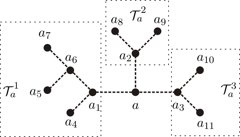
Figure 24: A tree graph where $a$ is connected with three subtrees $\mathcal{T}_{a}^{1}$, $\mathcal{T}_{a}^{2}$ and $\mathcal{T}_{a}^{3}$.

In general, the LHS of graph-based BCJ relation eq. (6.1) for an arbitrary tree $\mathcal{T}$ can be expanded in terms of the LHS of BCJ relations eq. (2.10). Particularly, we pick out an arbitrary node $a\in\mathcal{T}$ and assume that there are $N$ subtrees attached to $a$, say $\mathcal{T}_{a}^{1}$, $\mathcal{T}_{a}^{2}$,…,$\mathcal{T}_{a}^{N}$. The corresponding nodes adjacent to $a$ in $\mathcal{T}_{a}^{1}$, $\mathcal{T}_{a}^{2}$,…,$\mathcal{T}_{a}^{N}$ are $a_{1}$, $a_{2}$, …, $a_{N}$. We will prove that the LHS of eq. (6.1) can be expanded as

$$~{}~{}~{}\mathcal{B}^{a}_{G}\left(1\left|{\begin{minipage}{51.21504pt} \includegraphics[width=73.97733pt]{GraphBasedGEN1.jpg} \end{minipage}}~{}~{}~{}~{}~{}~{}~{},\boldsymbol{\gamma}\right|r\right)$$ (6.26)

$$= \mathcal{B}^{(1)}_{G}\left(1\left|{\begin{minipage}{51.21504pt} \includegraphics[width=73.97733pt]{GraphBasedGEN1.jpg} \end{minipage}}~{}~{}~{}~{}~{}~{}~{}\Bigg{|}_{a},\boldsymbol{\gamma}\right|r\right)+\sum\limits_{\shuffle}\mathcal{B}^{(2)}_{G}\left(1\left|{\begin{minipage}{45.52458pt} \includegraphics[width=62.59596pt]{GraphBasedGEN2.jpg} \end{minipage}}~{}~{}~{}~{}~{},\{a\}\shuffle\boldsymbol{\gamma}\right|r\right).$$

The first term of eq. (6.26) is the following combination

$$\mathcal{B}^{(1)}_{G}\left(1\left|{\begin{minipage}{51.21504pt} \includegraphics[width=73.97733pt]{GraphBasedGEN1.jpg} \end{minipage}}~{}~{}~{}~{}~{}~{}~{}\Bigg{|}_{a},\boldsymbol{\gamma}\right|r\right)\equiv\sum\limits_{\boldsymbol{\zeta}}\mathcal{B}\left(1\left|\boldsymbol{\zeta}\in{\begin{minipage}{51.21504pt} \includegraphics[width=73.97733pt]{GraphBasedGEN1.jpg} \end{minipage}}~{}~{}~{}~{}~{}~{}~{}\Bigg{|}_{a},\boldsymbol{\gamma}\right|r\right)$$ (6.27)

in which all nodes of $\mathcal{T}$ are in the $\boldsymbol{\beta}$ set. The second term of eq. (6.26) is a proper combination of BCJ relations eq. (6.1) where the node $a$ is always in the $\boldsymbol{\alpha}$ set. The explicit expression of this part can be determined recursively. In the following, we will assume eq. (6.26) holds for all subtrees $\mathcal{T}_{a}^{1}$, $\mathcal{T}_{a}^{2}$, …,$\mathcal{T}_{a}^{N}$ and prove eq. (6.26) by induction.

To prove eq. (6.26), we first show that $\mathcal{B}^{a}_{G}(1|\mathcal{T},\boldsymbol{\gamma}|r)$ can be expressed by those $\mathcal{B}^{a}_{G}$’s with subtrees $\mathcal{T}_{a}^{1},\dots,\mathcal{T}_{a}^{N}$ connecting to the node $a$. Let us explain this point explicitly by considering the example with $\mathcal{T}=\text{Fig.~{}\ref{Fig:GraphBasedGEN1-1}}$. According to the definition, $\mathcal{B}^{a}_{G}\left(1\left|\mathcal{T}=\text{Fig.~{}\ref{Fig:GraphBasedGEN1-1}},\boldsymbol{\gamma}\right|r\right)$ can be written as

$$\mathcal{B}^{a}_{G}\left(1\left|\mathcal{T}=\text{Fig.~{}\ref{Fig:GraphBasedGEN1-1}},\boldsymbol{\gamma}\right|r\right)=\Big{[}\sum\limits_{\boldsymbol{\sigma}}\sum\limits_{\boldsymbol{\zeta}\in\mathcal{T}|_{a}}(k_{a}\cdot Y_{a})+\sum\limits_{i=1}^{3}\sum\limits_{c\in\mathcal{T}_{a}^{i}}f^{c}\sum\limits_{\boldsymbol{\sigma}}\sum\limits_{\boldsymbol{\zeta}\in\mathcal{T}|_{c}}(k_{c}\cdot Y_{c})\Big{]}A(1,\boldsymbol{\sigma}\in(\boldsymbol{\zeta}\shuffle\boldsymbol{\gamma}),r).$$ (6.28)

Here $a_{1}$, $a_{2}$ and $a_{3}$ are the nearest-to-$a$ nodes which belong to substructures $\mathcal{T}_{a}^{1}$, $\mathcal{T}_{a}^{2}$ and $\mathcal{T}_{a}^{3}$ correspondingly. The total contributions from nodes in $\mathcal{T}_{a}^{1}$ (i.e. contributions with $i=1$ in the second term of eq. (6.28)) is given by

$$\sum\limits_{i\in\mathcal{T}_{a}^{1}}f^{i}\sum\limits_{\boldsymbol{\zeta}^{(1)}\in\mathcal{T}_{a}^{1}|_{i}}\Bigl{[}\sum\limits_{\boldsymbol{\zeta}^{(2)}\in\mathcal{T}_{a}^{2}|_{a_{2}}}\sum\limits_{\boldsymbol{\zeta}^{(3)}\in\mathcal{T}_{a}^{3}|_{a_{3}}}\sum\limits_{\shuffle}\sum\limits_{\boldsymbol{\sigma}}(k_{i}\cdot Y_{i})A\big{(}1,\boldsymbol{\sigma}\in(\boldsymbol{\zeta}^{(1)}\shuffle^{\prime}\{a,\boldsymbol{\zeta}^{(2)}\shuffle\boldsymbol{\zeta}^{(3)}\shuffle\boldsymbol{\gamma}\})\big{|}_{a_{1}\prec a},r\big{)}\Bigr{]},$$ (6.29)

where $\mathcal{T}_{a}^{2}|_{a_{2}}=\{a_{2},\{a_{8}\}\shuffle\{a_{9}\}\}$, $\mathcal{T}_{a}^{3}|_{a_{3}}=\{a_{3},\{a_{10}\}\shuffle\{a_{11}\}\}$. Permutations $\mathcal{T}_{a}^{1}|_{i}$ in eq. (6.29) are those established by the subgraph $\mathcal{T}_{a}^{1}$ when $i\in\mathcal{T}_{a}^{1}$ is considered as the leftmost element. Specifically,

$$\mathcal{T}_{a}^{1}|_{a_{1}} = \{a_{1},\{a_{4}\}\shuffle\{a_{6},\{a_{5}\}\shuffle\{a_{7}\}\}\},~{}\mathcal{T}_{a}^{1}|_{a_{4}}=\{a_{4},a_{1},a_{6},\{a_{5}\}\shuffle\{a_{7}\}\}$$ (6.30)

$$\mathcal{T}_{a}^{1}|_{a_{5}} = \{a_{5},a_{6},\{a_{7}\}\shuffle\{a_{1},a_{4}\}\},~{}\mathcal{T}_{a}^{1}|_{a_{6}}=\{a_{6},\{a_{5}\}\shuffle\{a_{7}\}\shuffle\{a_{1},a_{4}\}\},~{}\mathcal{T}_{a}^{1}|_{a_{7}}=\{a_{7},a_{6},\{a_{5}\}\shuffle\{a_{1},a_{4}\}\}.$$

For fixed permutations $\boldsymbol{\zeta}^{(2)}$, $\boldsymbol{\zeta}^{(3)}$ and a given permutation $\boldsymbol{\xi}\in\{a,\boldsymbol{\zeta}^{(2)}\shuffle\boldsymbol{\zeta}^{(3)}\}\shuffle\boldsymbol{\gamma}$, terms in eq. (6.29) are collected as

$$\sum\limits_{i\in\mathcal{T}_{a}^{1}}f^{i}\sum\limits_{\boldsymbol{\zeta}^{(1)}\in\mathcal{T}_{a}^{1}|_{i}}\sum\limits_{\boldsymbol{\sigma}}(k_{i}\cdot Y_{i})A\big{(}1,\boldsymbol{\sigma}\in(\boldsymbol{\zeta}^{(1)}\shuffle^{\prime}\boldsymbol{\xi})|_{a_{1}\prec a},r\big{)}=-\mathcal{B}^{a_{1}}_{G}\big{(}1\big{|}\mathcal{T}_{a}^{1},\boldsymbol{\xi}\big{|}r\big{)}.$$ (6.31)

Thus the sum of all contributions from $\mathcal{T}_{a}^{1}$ in eq. (6.29) reads (recall that $f^{a_{1}}=-f^{a}=-1$)

$$-\sum\limits_{\boldsymbol{\zeta}^{(2)}\in\mathcal{T}_{a}^{2}|_{a_{2}}}\sum\limits_{\boldsymbol{\zeta}^{(3)}\in\mathcal{T}_{a}^{3}|_{a_{3}}}\sum\limits_{\boldsymbol{\xi}\in\{a,\boldsymbol{\zeta}^{(2)}\shuffle\boldsymbol{\zeta}^{(3)}\}\shuffle\boldsymbol{\gamma}}\mathcal{B}^{a_{1}}_{G}\big{(}1\big{|}\mathcal{T}_{a}^{1},\boldsymbol{\xi}\big{|}r\big{)}.$$ (6.32)

Following similar discussions, the sum of contributions from $\mathcal{T}_{a}^{2}$ and $\mathcal{T}_{a}^{3}$ are respectively given by the replacements of labels $1\leftrightarrow 2$ and $1\leftrightarrow 3$. The expression eq. (6.28) is then expressed by terms with respect to subtree structures

$$\sum\limits_{\boldsymbol{\sigma}}\sum\limits_{\boldsymbol{\zeta}\in\mathcal{T}|_{a}}(k_{a}\cdot Y_{a})A(1,\boldsymbol{\sigma}\in(\boldsymbol{\zeta}\shuffle\boldsymbol{\gamma}),r)-\Bigl{[}\sum\limits_{\boldsymbol{\zeta}^{(2)}\in\mathcal{T}_{a}^{2}|_{a_{2}}}\sum\limits_{\boldsymbol{\zeta}^{(3)}\in\mathcal{T}_{a}^{3}|_{a_{3}}}\sum\limits_{\boldsymbol{\xi}\in\{a,\boldsymbol{\zeta}^{(2)}\shuffle\boldsymbol{\zeta}^{(3)}\}\shuffle\boldsymbol{\gamma}}\mathcal{B}^{a_{1}}_{G}\big{(}1\big{|}\mathcal{T}_{a}^{1},\boldsymbol{\xi}\big{|}r\big{)}$$

$$+ \sum\limits_{\boldsymbol{\zeta}^{(1)}\in\mathcal{T}_{a}^{1}|_{a_{1}}}\sum\limits_{\boldsymbol{\zeta}^{(3)}\in\mathcal{T}_{a}^{3}|_{a_{3}}}\sum\limits_{\boldsymbol{\xi}\in\{a,\boldsymbol{\zeta}^{(1)}\shuffle\boldsymbol{\zeta}^{(3)}\}\shuffle\boldsymbol{\gamma}}\mathcal{B}^{a_{2}}_{G}\big{(}1\big{|}\mathcal{T}_{a}^{2},\boldsymbol{\xi}\big{|}r\big{)}+\sum\limits_{\boldsymbol{\zeta}^{(2)}\in\mathcal{T}_{a}^{2}|_{a_{2}}}\sum\limits_{\boldsymbol{\zeta}^{(1)}\in\mathcal{T}_{a}^{1}|_{a_{1}}}\sum\limits_{\boldsymbol{\xi}\in\{a,\boldsymbol{\zeta}^{(2)}\shuffle\boldsymbol{\zeta}^{(1)}\}\shuffle\boldsymbol{\gamma}}\mathcal{B}^{a_{3}}_{G}\big{(}1\big{|}\mathcal{T}_{a}^{3},\boldsymbol{\xi}\big{|}r\big{)}\Bigr{]}.$$

The above discussion is naturally generalized to arbitrary tree structure $\mathcal{T}$. For any $\mathcal{B}^{a}_{G}$, we have

$$~{}~{}~{}~{}\mathcal{B}^{a}_{G}\left(1\left|{\begin{minipage}{51.21504pt} \includegraphics[width=73.97733pt]{GraphBasedGEN1.jpg} \end{minipage}}~{}~{}~{}~{}~{}~{}~{},\boldsymbol{\gamma}\right|r\right)$$

$$= \sum\limits_{\boldsymbol{\sigma}}\sum\limits_{\boldsymbol{\zeta}\in\mathcal{T}|_{a}}(k_{a}\cdot Y_{a})A(1,\boldsymbol{\sigma}\in(\boldsymbol{\zeta}\shuffle\boldsymbol{\gamma}),r)$$

$$- \biggl{[}\sum\limits_{\begin{subarray}{c}\boldsymbol{\zeta}^{(j)}\in\mathcal{T}_{a}^{j}|_{a_{j}}\\ \text{for}~{}j=2,\dots,N\end{subarray}}\sum\limits_{\shuffle}\mathcal{B}^{a_{1}}_{G}\bigl{(}1\big{|}\mathcal{T}_{a}^{1},\bigl{\{}a,\bcancel{\boldsymbol{\zeta}^{(1)}}\shuffle\boldsymbol{\zeta}^{(2)}\shuffle\dots\shuffle\boldsymbol{\zeta}^{(N)}\bigr{\}}\shuffle\boldsymbol{\gamma}\big{|}r\bigr{)}\big{|}_{a_{1}\prec a}$$

$$~{}~{}~{}~{}~{}~{}~{}+\sum\limits_{\begin{subarray}{c}\boldsymbol{\zeta}^{(j)}\in\mathcal{T}_{a}^{j}|_{a_{j}}\\ \text{for}~{}j=1,3,\dots,N\end{subarray}}\sum\limits_{\shuffle}\mathcal{B}^{a_{2}}_{G}\bigl{(}1\big{|}\mathcal{T}_{a}^{2},\bigl{\{}a,\boldsymbol{\zeta}^{(1)}\shuffle\bcancel{\boldsymbol{\zeta}^{(2)}}\shuffle\dots\shuffle\boldsymbol{\zeta}^{(N)}\bigr{\}}\shuffle\boldsymbol{\gamma}\big{|}r\bigr{)}\big{|}_{a_{2}\prec a}$$

$$+ ~{}\dots~{}+\sum\limits_{\begin{subarray}{c}\boldsymbol{\zeta}^{(j)}\in\mathcal{T}_{a}^{j}|_{a_{j}}\\ \text{for}~{}j=1,\dots,N-1\end{subarray}}\sum\limits_{\shuffle}\mathcal{B}^{a_{N}}_{G}\bigl{(}1\big{|}\mathcal{T}_{a}^{N},\bigl{\{}a,\boldsymbol{\zeta}^{(1)}\shuffle\boldsymbol{\zeta}^{(2)}\shuffle\dots\shuffle\bcancel{\boldsymbol{\zeta}^{(N)}}\bigr{\}}\shuffle\boldsymbol{\gamma}\big{|}r\bigr{)}\big{|}_{a_{N}\prec a}\biggr{]},$$

where we wrote the sum over multi-shuffle permutations by $\sum\limits_{\shuffle}$ for short. According to the inductive assumption, each term in the square brackets for a given $i$ can be expressed by the sum of the following two terms:

$$\sum\limits_{\begin{subarray}{c}\boldsymbol{\zeta}^{(j)}\in\mathcal{T}_{a}^{j}|_{a_{j}}\\ \text{for}~{}j=1,\dots,N,j\neq i\end{subarray}}\sum\limits_{\boldsymbol{\xi}^{(i)}}\mathcal{B}^{(1)}_{G}\bigl{(}1\big{|}\mathcal{T}_{a}^{i}\big{|}_{a_{i}},\boldsymbol{\xi}^{(i)}\big{|}r\bigr{)}\big{|}_{a_{i}\prec a} = \sum\limits_{\begin{subarray}{c}\boldsymbol{\zeta}^{(j)}\in\mathcal{T}_{a}^{j}|_{a_{j}}\\ \text{for}~{}j=1,\dots,N\end{subarray}}\sum\limits_{\boldsymbol{\xi}^{(i)}}\biggl{[}\mathcal{B}\bigl{(}1\big{|}\boldsymbol{\zeta}^{(i)},\boldsymbol{\xi}^{(i)}\big{|}r\bigr{)}-\mathcal{B}\bigl{(}1\big{|}\boldsymbol{\zeta}^{(i)},\boldsymbol{\xi}^{(i)}\big{|}r\bigr{)}\big{|}_{a_{i}\succ a}\biggr{]}$$

and

$$\sum\limits_{\begin{subarray}{c}\boldsymbol{\zeta}^{(j)}\in\mathcal{T}_{a}^{j}|_{a_{j}}\\ \text{for}~{}j=1,\dots,N,j\neq i\end{subarray}}\sum\limits_{\boldsymbol{\xi}^{(i)}}\biggl{[}\sum\limits_{\shuffle}\mathcal{B}^{(2)}_{G}\bigl{(}1\big{|}\mathcal{T}_{a}^{i}-a_{i},\{a_{i}\}\shuffle\boldsymbol{\xi}^{(i)}\big{|}r\bigr{)}\big{|}_{a_{i}\prec a}\biggr{]}.$$ (6.36)

In eq. (6.2) and eq. (6.36), the summations over $\boldsymbol{\xi}^{(i)}$ are taken by summing over all

$$\boldsymbol{\xi}^{(i)}\in\big{\{}\bigl{\{}{a,\boldsymbol{\zeta}^{(1)}\shuffle\dots\shuffle\bcancel{\boldsymbol{\zeta}^{(i)}}\shuffle\dots\shuffle\boldsymbol{\zeta}^{(N)}}\bigr{\}}\shuffle\boldsymbol{\gamma}\big{\}},$$ (6.37)

Eq. (6.2) is then given by summing the following two contributions together

• The sum of all the last terms on the RHS of eq. (6.2) for all $i=1,\dots,N$ and the first term of eq. (6.2)    According to eq. (2.11), the last term in the brackets of eq. (6.2) for given $\boldsymbol{\zeta}^{(j)}\in\mathcal{T}_{a}^{j}|_{a_{j}}$ ($j=1,2,\dots,N$) when summing over $\boldsymbol{\xi}^{(i)}$ can be explicitly written as

  $$\sum\limits_{\boldsymbol{\xi}^{(i)}}\mathcal{B}\bigl{(}1\big{|}\boldsymbol{\zeta}^{(i)},\boldsymbol{\xi}^{(i)}\big{|}r\bigr{)}\big{|}_{a_{i}\succ a}=\sum\limits_{\boldsymbol{\xi}^{(i)}}\sum\limits_{\boldsymbol{\eta}\in\boldsymbol{\zeta}^{(i)}\shuffle\boldsymbol{\xi}^{(i)}|_{a_{i}\succ a}}\sum\limits_{x\in\boldsymbol{\zeta}^{(i)}}(k_{x}\cdot X_{x}(\boldsymbol{\eta}))A(1,\boldsymbol{\eta},r).$$ (6.38)

  Here, $\sum\limits_{\boldsymbol{\xi}^{(i)}}\sum\limits_{\boldsymbol{\eta}\in\boldsymbol{\zeta}^{(i)}\shuffle\boldsymbol{\xi}^{(i)}|_{a_{i}\succ a}}$ is given by summing over permutations

  $$\bigl{(}\boldsymbol{\zeta}^{(i)}\shuffle\big{\{}\bigl{\{}{a,\boldsymbol{\zeta}^{(1)}\shuffle\dots\shuffle\bcancel{\boldsymbol{\zeta}^{(i)}}\shuffle\dots\shuffle\boldsymbol{\zeta}^{(N)}}\bigr{\}}\shuffle\boldsymbol{\gamma}\big{\}}\bigr{)}\big{|}_{a_{i}\succ a}.$$ (6.39)

  Recalling that $a_{i}$ is the leftmost element in $\boldsymbol{\zeta}^{(i)}\in\mathcal{T}_{a}^{i}|_{a_{i}}$, the above expression turns to

  $$\bigl{\{}{a,\boldsymbol{\zeta}^{(1)}\shuffle\dots\shuffle{\boldsymbol{\zeta}^{(i)}}\shuffle\dots\shuffle\boldsymbol{\zeta}^{(N)}}\bigr{\}}\shuffle\boldsymbol{\gamma}.$$ (6.40)

  Therefore, the sum of all the last terms of in eq. (6.2) over all $i=1,\dots,N$ and the first term of eq. (6.2) gives

  $$\sum\limits_{\begin{subarray}{c}\boldsymbol{\zeta}^{(j)}\in\mathcal{T}_{a}^{j}|_{a_{j}}\\ \text{for}~{}j=1,\dots,N\end{subarray}}\sum\limits_{\begin{subarray}{c}\boldsymbol{\eta}\in\{a,\boldsymbol{\zeta}^{(1)}\shuffle\dots\\ \shuffle{\boldsymbol{\zeta}^{(i)}}\shuffle\dots\shuffle\boldsymbol{\zeta}^{(N)}\}\end{subarray}}\left[\Big{(}\sum\limits_{i=1}^{N}\sum\limits_{x\in\boldsymbol{\zeta}^{(i)}}k_{x}\cdot X_{x}(\boldsymbol{\eta})\Big{)}+k_{a}\cdot X_{a}(\boldsymbol{\eta})\right]A(1,\boldsymbol{\eta}\shuffle\boldsymbol{\gamma},r)$$ (6.41)

  $$= \sum\limits_{\begin{subarray}{c}\boldsymbol{\zeta}^{(j)}\in\mathcal{T}_{a}^{j}|_{a_{j}}\\ \text{for}~{}j=1,\dots,N\end{subarray}}\sum\limits_{\shuffle}\mathcal{B}\bigl{(}1\big{|}\bigl{\{}a,\boldsymbol{\zeta}^{(1)}\shuffle\dots\shuffle\boldsymbol{\zeta}^{(N)}\bigr{\}},\boldsymbol{\gamma}\big{|}r\bigr{)}$$

  $$= \sum\limits_{\boldsymbol{\zeta}}\mathcal{B}\left(1\left|\boldsymbol{\zeta}\in{\begin{minipage}{51.21504pt} \includegraphics[width=73.97733pt]{GraphBasedGEN1.jpg} \end{minipage}}~{}~{}~{}~{}~{}~{}~{}\Bigg{|}_{a},\boldsymbol{\gamma}\right|r\right),$$

  which is just $\mathcal{B}^{(1)}_{G}$ in eq. (6.26).

• The sum of the first term in eq. (6.2) and eq. (6.36) over all $i=1,\dots,N$   This part defines

  $$\sum\limits_{\shuffle}\mathcal{B}^{(2)}_{G}\left(1\left|{\begin{minipage}{45.52458pt} \includegraphics[width=62.59596pt]{GraphBasedGEN2.jpg} \end{minipage}}~{}~{}~{}~{}~{},\{a\}\shuffle\boldsymbol{\gamma}\right|r\right)$$

  $$= \sum\limits_{i=1}^{N}\sum\limits_{\begin{subarray}{c}\boldsymbol{\zeta}^{(j)}\in\mathcal{T}_{a}^{j}|_{a_{j}}\\ \text{for}~{}j=1,\dots,N,j\neq i\end{subarray}}\sum\limits_{\boldsymbol{\xi}^{(i)}}\biggl{[}\sum\limits_{\boldsymbol{\zeta}^{(i)}}\mathcal{B}\bigl{(}1\big{|}\boldsymbol{\zeta}^{(i)}\in\mathcal{T}_{a}^{i}\big{|}_{a_{i}},\boldsymbol{\xi}^{(i)}\big{|}r\bigr{)}+\sum\limits_{\shuffle}\mathcal{B}^{(2)}_{G}\bigl{(}1\big{|}\mathcal{T}_{a}^{i}-a_{i},\{a_{i}\}\shuffle\boldsymbol{\xi}^{(i)}\big{|}r\bigr{)}\big{|}_{a_{i}\prec a}\biggr{]},$$

  where $\boldsymbol{\xi}^{(i)}$ is summed over all permutations satisfying eq. (• ‣ 6.2). In the square brackets, the first term is precisely the LHS of BCJ relation eq. (2.10) where $a$ is in the $\boldsymbol{\alpha}$ set. According to the inductive assumption, the second term is a combination of BCJ relations where both $a_{i}$ is in the $\boldsymbol{\alpha}$ set. Since $a\in\boldsymbol{\xi}^{(i)}$, $a$ must also be in the $\boldsymbol{\alpha}$ set. Thus the second term of eq. (• ‣ 6.2) is a combination of the LHS of those BCJ relations with $a_{i}\prec a$.

All together, we have proven that the LHS of the graph-based BCJ relation is a combination of the LHS of traditional BCJ relations.

7 Gauge invariance identities of tree-level YM and GR amplitudes

A tree level $n$ graviton amplitude $M(1,2,\dots,n)$ can be expanded as a combination of tree level single-trace EYM amplitudes. Particularly, we can pick out arbitrary two gravitons, for example, $1$ and $n$ and then write the amplitude $M(1,2,\dots,n)$ in terms of single-trace EYM amplitudes, where $1$ and $n$ are always considered as two gluons, as follows

$$M(1,2,\dots,n) = \sum\limits_{\text{Splits}}\,\sum\limits_{\boldsymbol{\sigma}\in\text{perms}\,\mathsf{A}}(-1)^{|\mathsf{A}|}\big{(}\epsilon_{1}\cdot F_{\sigma(1)}\cdot\dots\cdot F_{\sigma(|\mathsf{A}|)}\cdot\epsilon_{n}\big{)}A(1,\boldsymbol{\sigma},n\|\,{\mathsf{H}}).$$ (7.1)

Here, $|\mathsf{A}|$ is the number of elements in $\mathsf{A}$. We have summed over all splits $\{2,\dots,n-1\}\to\mathsf{A},\mathsf{H}$ in the first summation. For a given $\mathsf{A}$, we summed over all possible permutations $\boldsymbol{\sigma}$ of elements in $\mathsf{A}$. When the EYM amplitudes in eq. (7.1) are expressed by eq. (2.4), eq. (7.1) is then expanded in terms of pure YM amplitudes

$$M(1,2,\dots,n) = \sum\limits_{\text{Splits}}\,\sum\limits_{\boldsymbol{\sigma}\in\text{perms}\,\mathsf{A}}\sum\limits_{\boldsymbol{\xi}\,\in\,\boldsymbol{\sigma}\shuffle\,\text{perms}\,{\mathsf{H}}}W(1,\boldsymbol{\sigma},n)\mathcal{C}(1,\boldsymbol{\xi},n)A(1,\boldsymbol{\xi},n),$$ (7.2)

where

$$W(1,\boldsymbol{\sigma},n)\equiv\epsilon_{n}\cdot F_{\sigma(|\mathsf{A}|)}\cdot\dots\cdot F_{\sigma(1)}\cdot\epsilon_{1}.$$ (7.3)

The factor $(-1)^{|\mathsf{A}|}$ in eq. (7.1) is absorbed when the antisymmetry of the strength tensors are considered. If we collect all coefficients $n_{1|\boldsymbol{\zeta}|n}$ corresponding to a given permutation $\boldsymbol{\zeta}$ of elements in $\{2,\dots,n-1\}$ together, a more brief form (dual DDM form) is obtained

$$M(1,2,\dots,n)=\sum\limits_{\boldsymbol{\zeta}\in S_{n-2}}n_{1|\boldsymbol{\zeta}|n}A(1,\boldsymbol{\zeta},n),$$ (7.4)

where $n_{1|\boldsymbol{\zeta}|n}$ are the BCJ numerators corresponding to half-ladder diagrams.

The gauge invariance condition for any graviton $a$ states that the GR amplitude $M(1,2,\dots,n)$ must vanish under the replacement $\epsilon_{a}\to k_{a}$. If the graviton $a$ belongs to $\{2,\dots,n-1\}$, it can be an element of either $\mathsf{A}$ or $\mathsf{H}$ for a given split in eq. (7.1). For the former case, the gauge invariance is already included in the coefficients $W(1,\boldsymbol{\sigma},n)$ due to the antisymmetry of the strength tensors. For the latter case, $a$ is considered as a graviton in an EYM amplitude whose gauge invariance induced identity has been studied in the previous sections. Therefore, only the identity induced by the gauge invariance condition for $a=1\,\text{or}\,n$ requires further study.

In the following, we review the old-version graphic rule for the construction of BCJ numerators $n_{1|\boldsymbol{\zeta}|n}$ in eq. (7.4). Then we expand these graphs by refined graphs and prove that the gauge invariance induced identity

$$\sum\limits_{\boldsymbol{\zeta}\in S_{n-2}}n_{1|\boldsymbol{\zeta}|n}\big{|}_{\epsilon_{1}\to k_{1}}A(1,\boldsymbol{\zeta},n)=0~{}~{}$$ (7.5)

is a combination of BCJ relations. The identity induced by the condition $\epsilon_{n}\to k_{n}$ can be studied in a similar way. Once all GR, EYM and YM amplitudes are replaced by YM, YMS (Yang-Mills scalar) and BS (biscalar) amplitudes correspondingly, the discussions are immediately extended to the identities (for BS amplitudes) induced by the gauge invariance of YM amplitudes.

7.1 The old-version graphic rule for the BCJ numerators $n_{1|\boldsymbol{\zeta}|n}$

BCJ numerators $n_{1|\boldsymbol{\zeta}|n}$ obtained from eq. (7.2) can be constructed according to the following (old fasion) graphic rule Du:2017kpo :

Step-1  Define a reference order of elements $2$, $3$, …, $n-1$, $n$ by $\mathsf{R}=\{\rho(2),\rho(3),\dots,\rho(n-1),n\}$ where the graviton $n$ is considered the last element, $\boldsymbol{\rho}$ is a permutation of $2$, $3$, …, $n-1$. Define weight of elements $2$, $3$, …, $n-1$, $n$ by their positions in $\mathsf{R}$.

Step-2  For a given permutation $\boldsymbol{\zeta}$, pick out $i_{1}$, $i_{2}$, …, $i_{j}$ and $n$ from $\mathsf{R}=\{\rho(2),\rho(3),\dots,\rho(n-1),n\}$ such that the following condition is satisfied

$$\zeta^{-1}(1)<\zeta^{-1}(i_{1})<\dots<\zeta^{-1}(i_{j})<\zeta^{-1}(n).$$ (7.6)

Then we construct a chain $\mathbb{CH}=[n,i_{j},i_{j-1},\dots,i_{1},1]$ which starts from the node $n$, passes through internal nodes $i_{j}$, …, $i_{1}$ and ended at $1$. The node $1$ is considered as the root. The factor corresponding to the chain $\mathbb{CH}=[n,i_{j},i_{j-1},\dots,i_{1},1]$ is

$$W(1,i_{1},\dots,i_{j},n)=\epsilon_{n}\cdot F_{i_{j}}\cdot\dots\cdot F_{i_{1}}\cdot\epsilon_{1}.$$ (7.7)

Redefine the reference order by $\mathsf{R}\to\mathsf{R}^{\prime}=\mathsf{R}\setminus\{i_{1},\dots,i_{j},n\}\equiv\{\rho^{\prime}(1),\dots,\rho^{\prime}({n^{\prime}})\}$.

Step-3 Pick out $\rho^{\prime}(n^{\prime})$, $i^{\prime}_{1}$, …, $i^{\prime}_{j^{\prime}}$ from $\mathsf{R}^{\prime}$. Construct a chain $\mathbb{CH}=[\rho^{\prime}(n^{\prime}),i^{\prime}_{j^{\prime}},i^{\prime}_{j^{\prime}-1},\dots,i^{\prime}_{1},a]$ towards $a\in\{1\}\cup\{i_{1},i_{2},...,i_{j}\}$ (noting that $a$ cannot be $n$ because $n$ is always considered as the last element) such that

$$\zeta^{-1}(a)<\zeta^{-1}(i^{\prime}_{1})<\dots<\zeta^{-1}(i^{\prime}_{j^{\prime}})<\zeta^{-1}(\rho^{\prime}(n^{\prime}))$$ (7.8)

is satisfied. This chain corresponds to a factor

$$\epsilon_{\rho^{\prime}(n^{\prime})}\cdot F_{i^{\prime}_{j^{\prime}}}\cdot\dots F_{i^{\prime}_{1}}\cdot k_{a}.$$ (7.9)

Redefine the ordered set by $\mathsf{R}\to\mathsf{R}^{\prime\prime}=\mathsf{R}^{\prime}\setminus\{i^{\prime}_{1},\dots,i^{\prime}_{j^{\prime}},\rho^{\prime}(n^{\prime})\}\equiv\{\rho^{\prime\prime}(1),\dots,\rho^{\prime\prime}({n^{\prime\prime}})\}$.

Step-4  Repeat the above step. In each step, we define a chain which starts from the highest-weight element in the new defined $\mathsf{R}$ and ends at any node on chains constructed previously except the node $n$ (the root $1$ should be included). Redefine $\mathsf{R}$ by removing the starting and internal nodes which have been used in the current step. This process is terminated when $\mathsf{R}$ is empty. All chains together form a connected tree graph with the root $1$. Multiplying all factors corresponding to the chains and summing over all possible graphs for the permutation $\boldsymbol{\zeta}$, we finally get the BCJ numerator $n_{1|\boldsymbol{\zeta}|n}$.

7.2 Understanding the gauge invariance induced identity eq. (7.5)

When the condition $\epsilon_{1}\to k_{1}$ is imposed and all strength tensors $F_{i}^{\mu\nu}$ are expanded explicitly according to the definition eq. (2.3), the three types of chains (see Fig. 3) are distinguished. Hence the old-version graphic rule becomes a refined rule. The coefficients $n_{1|\boldsymbol{\zeta}|n}\big{|}_{\epsilon_{1}\to k_{1}}$ in the identity eq. (7.5) is then provided by

$$n_{1|\boldsymbol{\zeta}|n}\big{|}_{\epsilon_{1}\to k_{1}}=\sum\limits_{\mathcal{F}\in\widetilde{\mathbb{G}}(1,\boldsymbol{\zeta},n)}{\widetilde{\mathcal{D}}}^{[\mathcal{F}]},$$ (7.10)

where $\widetilde{\mathbb{G}}(1,\boldsymbol{\zeta},n)$ is the set of physical graphs defined by the refined graphic rule and we summed over all possible graphs $\mathcal{F}\in\widetilde{\mathbb{G}}(1,\boldsymbol{\zeta},n)$. The factor ${\widetilde{\mathcal{D}}}^{[\mathcal{F}]}$ denotes the coefficient for a given graph constructed by the refined rule. The identity eq. (7.5) then turns to

$$\sum\limits_{\boldsymbol{\zeta}\in S_{n-2}}\left[\sum\limits_{\mathcal{F}\in\widetilde{\mathbb{G}}(1,\boldsymbol{\zeta},n)}{\widetilde{\mathcal{D}}}^{[\mathcal{F}]}\right]A(1,\boldsymbol{\zeta},n)=0~{}~{}.$$ (7.11)

Before showing the relationship between the identity eq. (7.11) and BCJ relation eq. (2.10), we point out the following features of graphs $\mathcal{F}$ in eq. (7.11):

• For any permutation $1,\boldsymbol{\zeta},n$, the nodes $1$ and $n$ are always the leftmost and the rightmost nodes respectively. The node $1$ always plays as the root of a graph $\mathcal{F}$. The node $n$ cannot be the end node of other chains.

• Since $\epsilon_{1}$ is replaced by $k_{1}$, the node $1$ must be connected by lines with arrows pointing to it. Hence only type-2 lines (with the arrows pointing to $1$) and type-3 lines can be connected to $1$.

• Any starting node of a chain is associated with a polarization, thus each of them starts a type-1 line or a type-2 line pointing towards the direction of the root.

• Being different from the graphs for the identity induced from EYM amplitudes, graphs that do not involve any type-3 line are allowed. In such a graph, all lines are type-2 lines pointing to the direction of the root $1$.

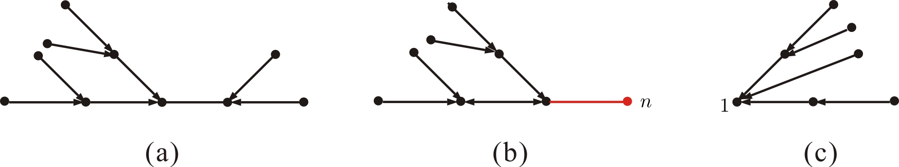
Figure 25: Graphs (a), (b) and (c) are correspondingly typical graphs of type-I, -II,-III components in the skeleton of the $T_{1}$ part in eq. (7.12).

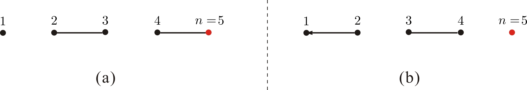
Figure 26: Graphs (a) and (b) are typical skeletons (with three components) for graphs contributing to $T_{1}$ and $T_{2}$ (see eq. (7.12)) with $n=5$, respectively. Here the reference order is chosen as $\mathsf{R}=\{1,2,3,4,5\}$. In graph (a), the type-1 line with its two ends $2$ and $3$, the type-1 line with its two ends $4$ and $5$, the single node $a$ are respectively type-I, -II and -III components. In graph (b), the type-2 line with its two ends $1$ and $2$ (the arrow points to $1$), the type-1 line with its ends $3$ and $4$, the single node $5$ are respectively type-I, -II and -III components.

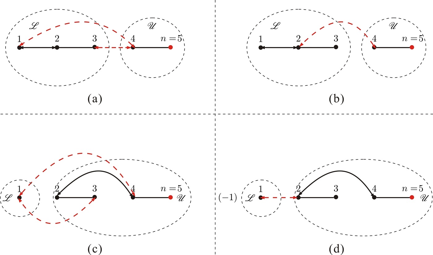
Figure 27: Graphs (a) and (c) are physical graphs corresponding to the skeleton Fig. 26 (a). They are obtained by constructing a chain of component, which starts from the type-I component, towards the lower and upper blocks respectively according to rule-2 (noting that the node $n$ cannot be the ending node of any chain). Thus there are two distinct configurations of the final upper and lower blocks $\mathscr{U}$ and $\mathscr{L}$. Spurious graphs are given by (b) and (d). Since the spurious component, whose only a single side (i.e. the node $2$) on the part from the highest weight node $5$ to the root $1$, belongs to the final upper block in (d), we should have an extra minus. Apparently graphs (b) and (d) cancel with each other.

To study eq. (7.11), we classify all graphs into two categories according to wether the node $n$ is connected by a type-1 line or a type-2 line. Then the LHS of $eq.~{}(\ref{Eq:GRYM3})$ is written as the sum of $T_{1}$ and $T_{2}$:

$$T_{1}\equiv\sum\limits_{\boldsymbol{\zeta}\in S_{n-2}}\left[\sum\limits_{\mathcal{F}\in\widetilde{\mathbb{G}}_{1}(1,\boldsymbol{\zeta},n)}{\widetilde{\mathcal{D}}}^{[\mathcal{F}]}\right]A(1,\boldsymbol{\zeta},n),~{}~{}~{}T_{2} \equiv \sum\limits_{\boldsymbol{\zeta}\in S_{n-2}}\left[\sum\limits_{\mathcal{F}\in\widetilde{\mathbb{G}}_{2}(1,\boldsymbol{\zeta},n)}{\widetilde{\mathcal{D}}}^{[\mathcal{F}]}\right]A(1,\boldsymbol{\zeta},n),$$ (7.12)

where $\widetilde{\mathbb{G}}_{1}(1,\boldsymbol{\zeta},n)$ and $\widetilde{\mathbb{G}}_{2}(1,\boldsymbol{\zeta},n)$ denote the set of graphs where $n$ is connected by a type-1 line and a type-2 line (pointing to the direction of root), respectively. We study these two parts separately.

The $T_{1}$ part  If the node $n$ is connected by a type-1 line, the chain $\mathbb{CH}=[n,i_{j},i_{j-1},\dots,i_{1},1]$ contributing to $T_{1}$ (see eq. (7.12)) can be described by Fig. 14 (b) when replacing the nodes $b$ and $h_{\rho(s)}$ therin respectively by the node $1$ and the node $i_{j}$ that is further connected by a type-1 line starting at the node $n$. According to discussions in section 5.1, such a chain must involve at least one type-3 line. As a result, the skeleton (the graph obtained by removing all type-3 lines) for a graph contributing to $T_{1}$ must be a disconnected graph. Following a similar discussion with section 5.1, we find that there are three types of components corresponding to a given skeleton in general (as in the EYM case):

• Type-I component: A component which contains neither $1$ nor $n$ and involves a type-1 line (see Fig. 25 (a))   In general, such a component can have type-2 lines whose arrows point to the direction of the ends of the type-1 line (i.e. the kernel).

• Type-II component: A component containing the node $n$ (see Fig. 25 (b))   Components of this type also have a kernel: the type-1 line with two ends $n$ and $a$ ($a\neq n,1$). The difference from type-I components is that all possible type-2 lines must be only on the bottom side (i.e. the side containing node $a$) of this component. The node $n$ is the starting node of the kernel (the type-1 line) of this component, while it cannot be the ending node of any chain. Thus there cannot be lines ended at $n$.

• Type-III component: A component containing the root $1$ (see Fig. 25 (c))   Such a component only involve type-2 lines whose arrows point to the direction of the root $1$.

A typical skeleton for graphs contributing to $T_{1}$ with $n=5$ is presented by Fig. 26 (a).

Having defined these three types of components, we can follow all the discussions in section 5 including the rule-1 and -2 for physical graphs as well as the construction and cancellation of spurious graphs (see Fig. 27 for the skeleton Fig. 26 (a)). The only thing we need to pay more attention to is that the node $n$ in the type-II component cannot be connected with nodes in other components via type-3 lines and it must be the rightmost element in any permutation. For any configuration of final upper and lower blocks, the sum of all physical graphs and spurious graphs is proportional to the LHS of the graph-based BCJ relation. For example, the sum of graphs Fig. 27 (a) and (b) provides $(-1)^{2}(\epsilon_{2}\cdot\epsilon_{3})(\epsilon_{4}\cdot\epsilon_{5})(k_{1}\cdot k_{2})\mathcal{B}^{4}_{G}\,\big{(}1\big{|}\includegraphics[width=4.26773pt]{GRYMEG4.jpg},\{2,3\}\big{|}5\big{)}$ while the sum of graphs (c) and (d) contributes $(\epsilon_{2}\cdot\epsilon_{3})(\epsilon_{4}\cdot\epsilon_{5})(k_{2}\cdot k_{4})\mathcal{B}^{3}_{G}\,\big{(}1\big{|}\includegraphics[width=45.52458pt]{GRYMEG3.jpg},\emptyset\big{|}5\big{)}$. Therefore, we conclude that the $T_{1}$ part can always be written as a combination of the LHS of graph-based BCJ relations eq. (6.1) which have been proven to be a combination of traditional BCJ relations eq. (2.10).

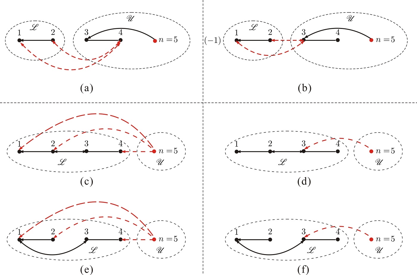
Figure 28: Graphs (a), (c) and (e) are physical graphs corresponding to the skeleton Fig. 26 (b). The type-I chain belongs to the final upper (lower) block in (a)((c)and (e)). Corresponding spurious graphs are given by (b), (d) and (f). The final upper block in (b) contains a spurious component (i.e. the type-I component), thus there should be an extra minus. In graphs (d) and (f), the final upper block does not contain any spurious component, thus the sign is plus. All spurious graphs (b), (d) and (f) cancel out (noting that (b) stands for two graphs).

The $T_{2}$ part  Graphs contributing to $T_{2}$ involve the node $n$ which is connected by a type-2 line (pointing towards the direction of root). To expand $T_{2}$ by BCJ relations, we should adjust the definition of skeleton by those graphs which are obtained by removing both type-3 lines and the type-2 line attached to the node $n$. Any skeleton under this definition is a disconnected graph. The definition of type-I and type-III components are same with those in the $T_{1}$ case. The type-II component is defined by the single node $n$. Along the line pointed in rule-2 in section 5, we define the upper and lower blocks by the maximally connected graphs containing the node $n$ and $1$ respectively. At the beginning, the upper and lower blocks are correspondingly the type-II and the type-III components. According to rule-2 in section 5.2, we attach a chain of components to either the upper or the lower bock and redefine these blocks in each step. In this case, we should require that the node $n$ can only be connected by the first chain that is attached to the upper block, via a type-2 line (with the arrows pointing towards root). When all components are used, we arrive the final upper and lower blocks. As done in section 5, we connect these two blocks into a fully connected graph:

• If the final upper block consists of more than one node, such as Fig. 28 (a), (b), we should connect a node $b$ in the final lower block with a node $a$ ($b\neq n$) in the final upper block via a type-3 line.

• If the final upper block only contains the node $n$, such as Fig. 28 (c), (d), (e) and (f), we should connect a node $b$ in the final lower block with $n$ via a type-2 line whose arrow points to $a$.

After this step, a graph is a spurious one (for example Fig. 28 (b), (d) and (f)) if it contains spurious components (whose only a single side is passed through by the path from $n$ to $1$), otherwise, it is a physical graph (for example Fig. 28 (a), (c) and (e)). The extra sign associated with a spurious graph is given by $(-1)^{\mathcal{S}(\mathscr{U})}$, where $\mathcal{S}(\mathscr{U})$ is the number of spurious components in the final upper block. Spurious graphs belonging to distinct final upper and lower blocks cancel in pairs as shown in section 5.3. For example the two graphs included by Fig. 28 (b) cancel with Fig. 28 (d) and (e), respectively. Hence, the $T_{2}$ can be given by summing over (1) all possible configurations of the final upper and lower blocks, (2) all possible graphs constructed by connecting these two blocks according to (i) and (ii) pointed above for a given configuration. Particularly,

• If the final upper block consists of more than one node, the sum of all graphs given by (i) is expanded in terms of the LHS of the graph-based BCJ relations eq. (6.1) (hence the LHS of traditional BCJ relations eq. (2.10)). For example the sum of graphs included in Fig. 28 (a) and (b) is proportional to the LHS of a graph-based BCJ relation $(-1)(\epsilon_{1}\cdot\epsilon_{2})(\epsilon_{3}\cdot\epsilon_{4})(\epsilon_{5}\cdot k_{3})B^{4}_{G}\big{(}1\big{|}\includegraphics[width=28.90755pt]{GRYMEG5.jpg},\{2\}\big{|}5\big{)}$.

• If the final upper block consists of only the node $n$, $n$ can be connected to any node $b$ in the final lower block via a type-2 line $\epsilon_{n}\cdot k_{a}$ (see Fig. 28 (c), (d) and (e), (f) for distinct configurations of the final lower block). The permutations established by graphs with all choices of $b$ are same. Thus we can extract a total factor

  $$\sum\limits_{a\in\{1,2,\dots,n-1\}}\epsilon_{n}\cdot k_{a}=\epsilon_{n}\cdot(-k_{n})=0,$$ (7.13)

  where the transversality of polarization and momentum conservation have been applied. Hence this part must vanish.

To sum up, the identity eq. (7.5) which is induced by the gauge invariance of gravity can always been expressed as a combination of BCJ relations.

8 Conclusions

In this paper, a graphic approach to the relationship between gauge invariance induced identity (where coefficients are polynomials of Lorentz inner products $\epsilon\cdot\epsilon$, $\epsilon\cdot k$ and $k\cdot k$) and BCJ relations (where coefficients are functions of only Mandelstam variables $k\cdot k$) is provided. By establishing a refined graphic rule, the three types of Lorentz inner products $\epsilon\cdot\epsilon$, $\epsilon\cdot k$ and $k\cdot k$ are represented by type-1, -2 and -3 lines correspondingly. To find out the relationship between the identity induced from the gauge invariance of tree level single-trace EYM amplitude and BCJ relations, we collected terms containing the same skeleton (the subgraph obtained by deleting all type-3 lines). We further proved that the sum of physical graphs for a given skeleton can be given by (a) summing over all possible configurations of final upper and lower blocks (defined by rule-2); (b) for a given configuration, summing over all possible (physical and spurious) graphs constructed by connecting a type-3 line between the final upper and lower blocks. Each summation in (b) is in fact proportional to a graph-based BCJ relation which was further proved to be a combination of traditional BCJ relations. Following a similar discussion, we proved that the identity induced by the gauge invariance of tree level GR (YM) amplitudes could also be expanded in terms of traditional BCJ relations.

We close this paper by presenting the following two related topics that deserve further study:

• First, how to extend the discussions to the identities induced from multi-trace EYM amplitudes? Two types of recursive expansion of tree level multi-trace EYM amplitudes were established in Du:2017gnh . Correspondingly, there are two identities (mentioned as type-I and II in Du:2017gnh ) induced by the gauge invariance condition of the fiducial graviton and the cyclic symmetry of a gluon trace. The type-II identity for amplitudes with two gluon traces and no graviton can be understood as the graph-based BCJ relation eq. (6.1) in which the tree graph $\mathcal{T}$ is a simple chain. However, this observation cannot be straightforwardly generalized to amplitudes with an arbitrary number of traces and gravitons. Thus the relationship between identities induced from arbitrary multi-trace EYM amplitudes still deserves further consideration.

• Second, how to calculate helicity amplitudes in four dimensions by the refined graphic rule? In four dimensions, the tree level single-trace EYM and GR amplitudes with maximally-helicity-violating (MHV) configurations were shown to be proportional to (Hodges) determinants (see Hodges:2012ym for GR and Du:2016wkt for EYM) which can be further expanded by graphs Nguyen:2009jk ; Feng:2012sy ; Du:2016wkt . Such brief formulas cannot be trivially extended to arbitrary helicity configurations. It is worth studying the relationship between the graphic expansion of the Hodges determinants Hodges:2012ym and the refined graphic expansion of amplitudes in the current paper. This may provide hints for finding simple formulas of EYM and GR amplitudes beyond MHV.

Appendix A Conventions and definitions

$\mathsf{H}$: the graviton set                             $F_{i}^{\mu\nu}$: the strength tensor $k_{i}^{\mu}\epsilon_{i}^{\nu}-\epsilon_{i}^{\mu}k_{i}^{\nu}$

Permutations: $\boldsymbol{\alpha},\boldsymbol{\beta},\boldsymbol{\rho},\boldsymbol{\sigma},\boldsymbol{\xi},\boldsymbol{\zeta}$   $\sigma(i)$: the $i$-th element in $\boldsymbol{\sigma}$   $\sigma^{-1}(l)$: the position of $l$ in permutation $\boldsymbol{\sigma}$

$\mathsf{A}\shuffle\mathsf{B}$ for ordered sets $\mathsf{A}$ and $\mathsf{B}$: permutations by merging $\mathsf{A}$ and $\mathsf{B}$ s.t. the relative order of elements in each set is kept, e.g. $\{1,2\}\shuffle\{a,b\}=\{\{1,2,a,b\},\{1,a,2,b\},\{1,a,b,2\},\{a,1,2,b\},\{a,1,b,2\},\{a,b,1,2\}\}$.

$Y_{i}(\boldsymbol{\sigma})$ for $\boldsymbol{\sigma}\in\boldsymbol{\alpha}\shuffle\boldsymbol{\beta}$ and $i\in\boldsymbol{\beta}$: the sum of all momenta of elements in $\boldsymbol{\sigma}$ (including the element $1$) on the LHS of $i$ in permutation $\boldsymbol{\sigma}$.

$X_{i}(\boldsymbol{\sigma})$ for $\boldsymbol{\sigma}\in\boldsymbol{\alpha}\shuffle\boldsymbol{\beta}$ and $i\in\boldsymbol{\beta}$: the sum of all momenta of elements in both $\boldsymbol{\beta}$ and $\boldsymbol{\alpha}$ (including the element $1$) that appear on the LHS of $i$ in permutation $\boldsymbol{\sigma}$.

$\mathcal{F}$: Graphs                          $\mathsf{R}=\{h_{\rho(1)},\dots,h_{\rho(s)}\}$: a reference order of gravitons $h_{1},\dots,h_{s}$

Weight of a graviton $h_{i}$: the position of $h_{i}$ in the reference order $\mathsf{R}$

$\mathbb{CH}=\left[a,i_{j},\dots,i_{1},b\right]$: a chain of nodes with starting node $a$, ending node $b$ and internal nodes $i_{1},\dots,i_{j}$

$\mathcal{B}(1\,|\,\boldsymbol{\beta},\boldsymbol{\alpha}\,|\,r)$: the LHS of BCJ relation eq. (2.10)

$\mathcal{B}^{\,c}_{G}(1\,|\,\mathcal{T},\boldsymbol{\gamma}\,|\,r)$: the LHS of the graph based BCJ relation eq. (6.1) with choosing $f^{c}=1$

Type-1, 2 and 3 lines: lines corresponding to factors of forms $\epsilon_{a}\cdot\epsilon_{b}$, $\epsilon_{a}\cdot k_{b}$ and $k_{a}\cdot k_{b}$ in the refined graphic rule

$\mathcal{F}^{\prime}\subset\mathcal{F}$: skeleton which is defined by removing all type-3 lines from a graph $\mathcal{F}$ for the relation

${\mathcal{F}\setminus\mathcal{F}^{\prime}}$ for eq. (3.1): the subgraph of $\mathcal{F}$ which is obtained by removing all lines of $\mathcal{F}^{\prime}$ from $\mathcal{F}$

$\mathcal{P}^{[\mathcal{F}^{\prime}]}$: coefficient associated to the skeleton $\mathcal{F}^{\prime}$     $\mathcal{K}^{[{\mathcal{F}\setminus\mathcal{F}^{\prime}}]}$: coefficient associated to the graph ${\mathcal{F}\setminus\mathcal{F}^{\prime}}$

$\mathcal{N}(\mathcal{F})$: the number of arrows (excluding the one which is attached to and points to the highest-weight node $h_{\rho(s)}$ in the gauge invariance induced identity eq. (3.1)) pointing deviate from the direction of roots.

$\boldsymbol{\sigma}^{\mathcal{F}}$: permutations allowed by graph $\mathcal{F}$

Type-I sector of a chain: A sector containing a type-1 line and possible type-2 lines whose arrows point to the two ends of the type-1 line

Type-II sector of a chain (the chain led by the highest weight node $h_{\rho(s)}$): A sector only containing type-2 lines whose arrows point to the direction of the starting node $h_{\rho(s)}$ of the chain.

Type-III sector of a chain: A sector only containing type-2 lines whose arrows point to the direction of the ending node of the chain

Type-I component $\mathscr{C}^{\text{I}}$: component containing a type-1 line and possible type-2 lines whose arrows pointing to the direction of the two ends of the type-1 line.

Kernel of a type-I component: the type-1 line in the type-I component

The top and bottom sides $\mathscr{C}^{\text{I}}_{t}$ and $\mathscr{C}^{\text{I}}_{b}$ of a type-I component $\mathscr{C}^{\text{I}}$: the two sides connected by the type-1 line. The side containing the highest-weight node in $\mathscr{C}^{\text{I}}$ is the top side $\mathscr{C}^{\text{I}}_{t}$. The side which does not contain the highest-weight node in $\mathscr{C}^{\text{I}}$ is the bottom side $\mathscr{C}^{\text{I}}_{b}$.

Type-II component $\mathscr{C}^{\text{II}}$: the component containing the highest-weight graviton $h_{\rho(s)}$.

Type-III component $\mathscr{C}^{\text{III}}$ : the component containing roots.

$\mathsf{R}_{\mathscr{C}}$: the reference order of components    The weight of a component: the position of a component in $\mathsf{R}_{\mathscr{C}}$

The upper and lower blocks $\mathscr{U}$ and $\mathscr{L}$ in rule-2: the maximally connected graphs involving the type-II and the type-III components $\mathscr{C}^{\text{II}}$ and $\mathscr{C}^{\text{III}}$ respectively.

$\mathcal{S}(\mathscr{U})$: the number of spurious components in the final upper block

$\mathcal{T}$: a tree graph with dashed lines (lines only imply the relative positions of nodes)

$\mathcal{T}|_{a}$: permutations established by $\mathcal{T}$ when considering $a$ as the leftmost node

$\oplus$: union of two disjoint graphs

$\mathcal{T}-\mathcal{T}^{\prime}$ for a graph $\mathcal{T}$ its subgraph $\mathcal{T}^{\prime}$: the graph obtained by removing all nodes in $\mathcal{T}^{\prime}$ and the lines attached to these nodes from $\mathcal{T}$

Appendix B Graphs for the $\mathsf{H}=11$ example

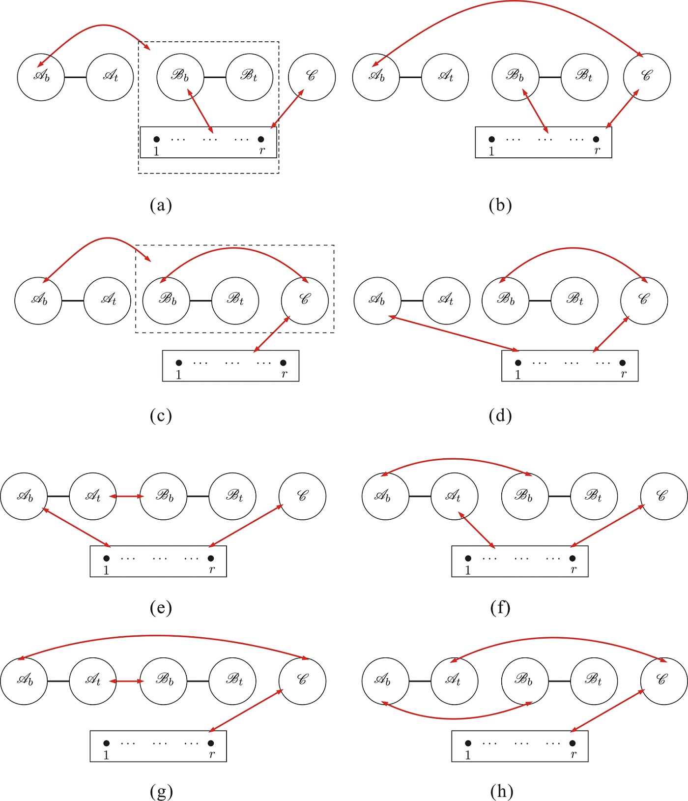
Figure 29: Physical graphs for the skeleton Fig. 16 by construction-1: part 1.

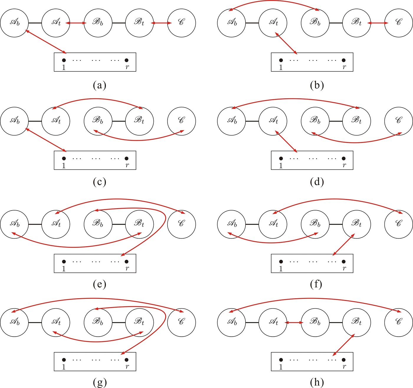
Figure 31: Physical graphs for the skeleton Fig. 16 by construction-1: part 3.

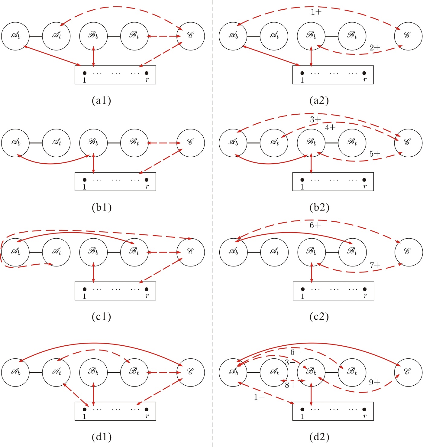
Figure 32: Physical graphs (a1), (b1), (c1), (d1) for the skeleton Fig. 16 by construction-2 and the corresponding spurious graphs (a2), (b2), (c2), (d2): part 1.

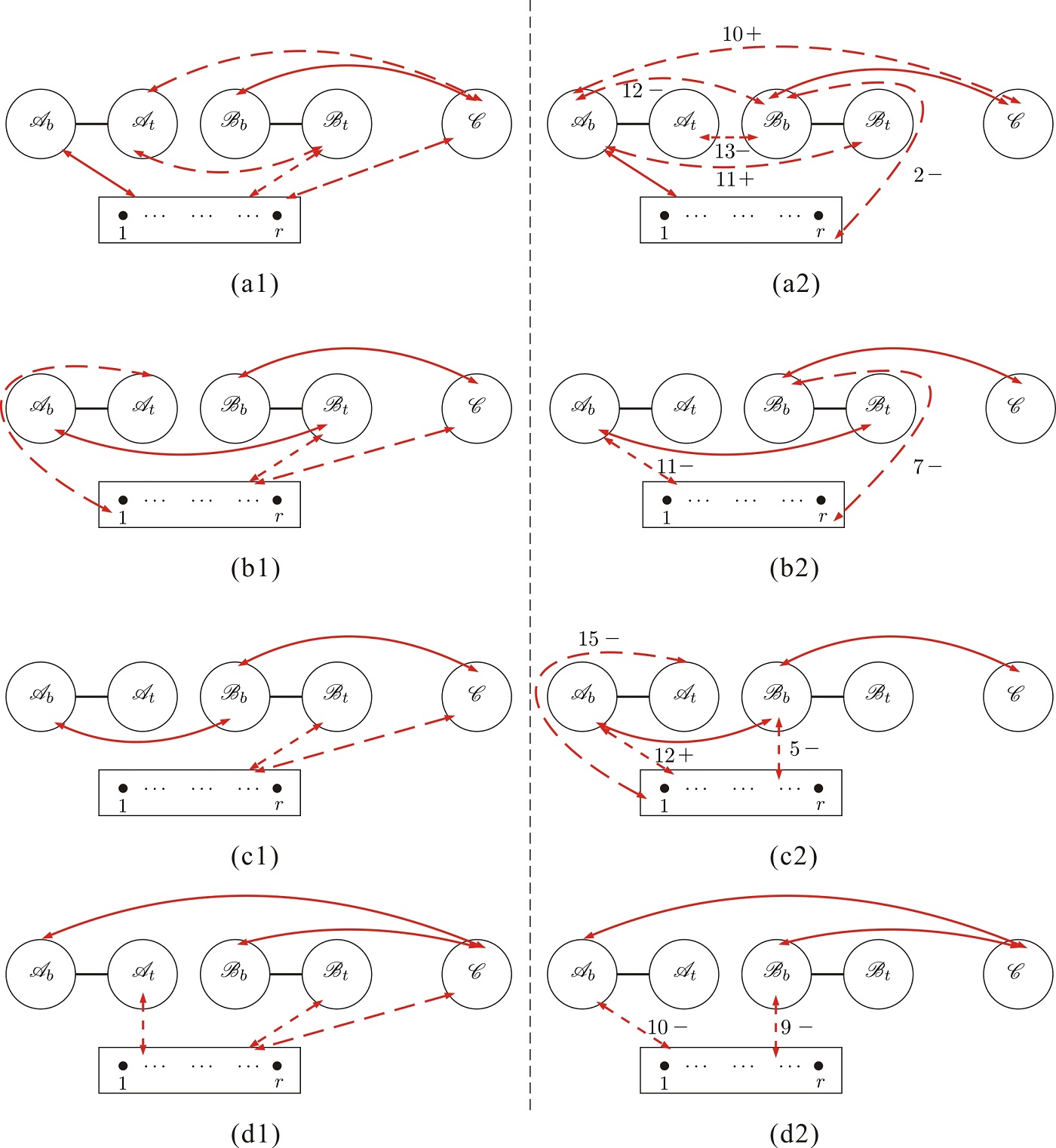
Figure 33: Physical graphs (a1), (b1), (c1), (d1) for the skeleton Fig. 16 by construction-2 and the corresponding spurious graphs (a2), (b2), (c2), (d2): part 2.

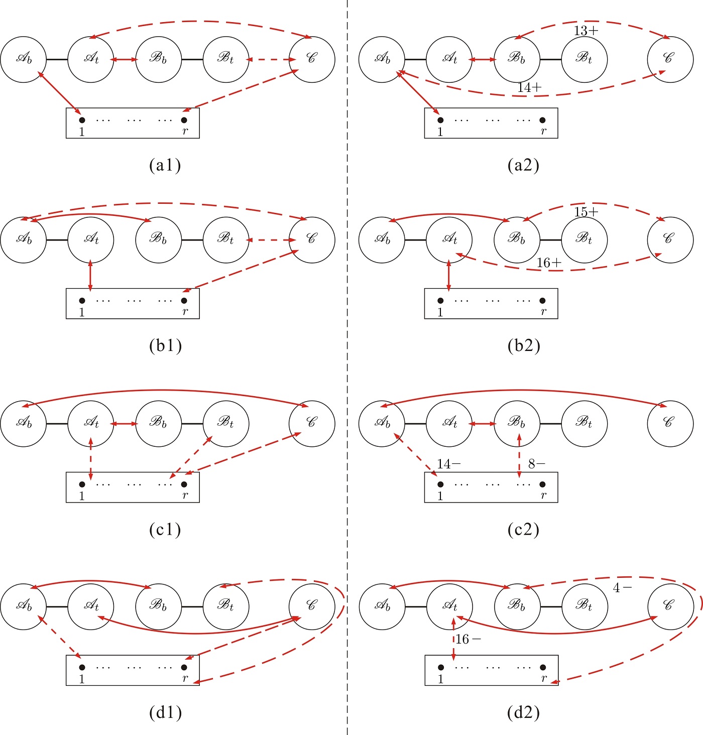
Figure 34: Physical graphs (a1), (b1), (c1), (d1) for the skeleton Fig. 16 by construction-2 and the corresponding spurious graphs (a2), (b2), (c2), (d2): part 3.

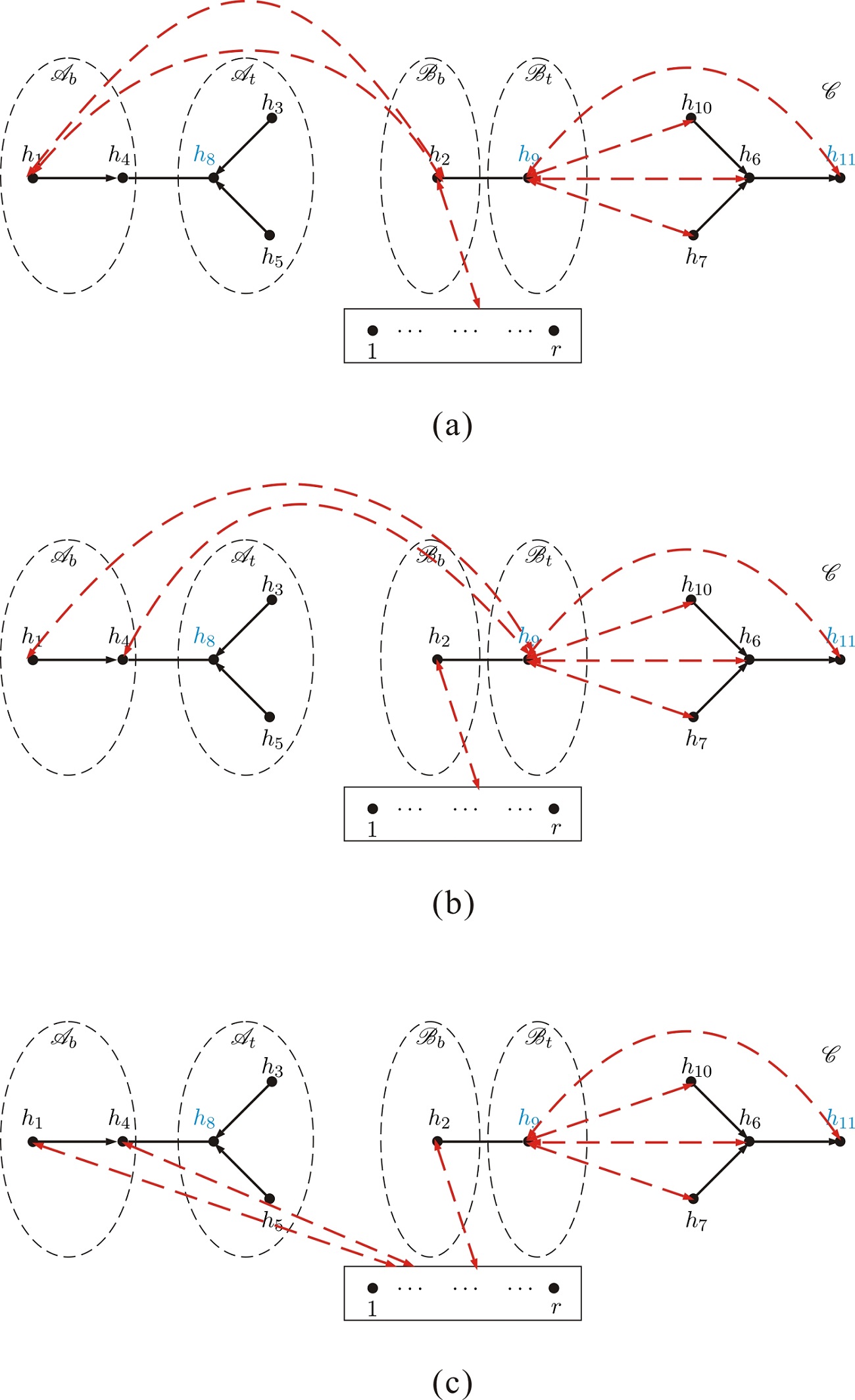
Figure 35: All possible graphs for Fig. 29 (a). In Fig. 29 (a), the $\mathscr{A}$ component can be connected with all the three regions $\mathscr{B}_{b}$ (see (a)), $\mathscr{B}_{t}$ (see (b)) and $\mathscr{C}$ (see (c)) in the dashed box.)

All physical graphs for the skeleton Fig. 16 obtained by construction-1 are displayed in figures (29), (30) and (31). In each graph, the inner structure in $\mathscr{C}$ and each side of $\mathscr{A}$ and $\mathscr{B}$ are neglected for convenience. Each type-3 line can be connected to arbitrary two nodes in the corresponding region. For example in Fig. 29 (a), the two end nodes of the type-three line between $\mathscr{A}_{b}$ and the dashed box can be an arbitrary node in $\mathscr{A}_{b}$ and an arbitrary node in $\mathscr{B}\oplus\mathscr{R}$ (except $n$ because in the expansion of EYM amplitude $n$ cannot play as a root). All graphs corresponding to Fig. 29 (a) are displayed in Fig. 35.

All physical graphs obtained by construction-2 are given by Fig. 32 (a1), (b1), (c1), (d1), Fig. 33 (a1), (b1), (c1), (d1) and Fig. 34 (a1), (b1), (c1), (d1). Each graph with a given dashed double arrow line gives a possible configuration. The corresponding spurious graphs are provided by Fig. 32 (a2), (b2), (c2), (d2), Fig. 33 (a2), (b2), (c2), (d2) and Fig. 34 (a2), (b2), (c2), (d2). The two spurious graphs with the dashed lines labeled by the same number but opposite signs cancel with each other.

References

- (1) R. H. Boels and R. Medina, Graviton and gluon scattering from first principles, Phys. Rev. Lett. 118 (2017) 061602, [arXiv:1607.08246].
- (2) N. Arkani-Hamed, L. Rodina, and J. Trnka, Locality and Unitarity from Singularities and Gauge Invariance, arXiv:1612.02797.
- (3) R. H. Boels and H. Luo, A minimal approach to the scattering of physical massless bosons, JHEP 05 (2018) 063, [arXiv:1710.10208].
- (4) R. H. Boels, Q. Jin, and H. Luo, Efficient integrand reduction for particles with spin, arXiv:1802.06761.
- (5) C.-H. Fu, Y.-J. Du, R. Huang, and B. Feng, Expansion of Einstein-Yang-Mills Amplitude, JHEP 09 (2017) 021, [arXiv:1702.08158].
- (6) M. Chiodaroli, M. Gunaydin, H. Johansson, and R. Roiban, Explicit Formulae for Yang-Mills-Einstein Amplitudes from the Double Copy, JHEP 07 (2017) 002, [arXiv:1703.00421].
- (7) F. Cachazo, S. He, and E. Y. Yuan, Scattering equations and Kawai-Lewellen-Tye orthogonality, Phys. Rev. D90 (2014), no. 6 065001, [arXiv:1306.6575].
- (8) F. Cachazo, S. He, and E. Y. Yuan, Scattering of Massless Particles in Arbitrary Dimensions, Phys. Rev. Lett. 113 (2014), no. 17 171601, [arXiv:1307.2199].
- (9) F. Cachazo, S. He, and E. Y. Yuan, Scattering of Massless Particles: Scalars, Gluons and Gravitons, JHEP 07 (2014) 033, [arXiv:1309.0885].
- (10) F. Cachazo, S. He, and E. Y. Yuan, Scattering Equations and Matrices: From Einstein To Yang-Mills, DBI and NLSM, JHEP 07 (2015) 149, [arXiv:1412.3479].
- (11) F. Teng and B. Feng, Expanding Einstein-Yang-Mills by Yang-Mills in CHY frame, JHEP 05 (2017) 075, [arXiv:1703.01269].
- (12) Y.-J. Du and F. Teng, BCJ numerators from reduced Pfaffian, JHEP 04 (2017) 033, [arXiv:1703.05717].
- (13) S. Stieberger and T. R. Taylor, New relations for Einstein-Yang-Mills amplitudes, Nucl. Phys. B913 (2016) 151–162, [arXiv:1606.09616].
- (14) D. Nandan, J. Plefka, O. Schlotterer, and C. Wen, Einstein-Yang-Mills from pure Yang-Mills amplitudes, JHEP 10 (2016) 070, [arXiv:1607.05701].
- (15) L. de la Cruz, A. Kniss, and S. Weinzierl, Relations for Einstein-Yang-Mills amplitudes from the CHY representation, Phys. Lett. B767 (2017) 86–90, [arXiv:1607.06036].
- (16) O. Schlotterer, Amplitude relations in heterotic string theory and Einstein-Yang-Mills, JHEP 11 (2016) 074, [arXiv:1608.00130].
- (17) Y.-J. Du, B. Feng, and F. Teng, Expansion of All Multitrace Tree Level EYM Amplitudes, arXiv:1708.04514.
- (18) R. Britto, F. Cachazo, and B. Feng, New recursion relations for tree amplitudes of gluons, Nucl. Phys. B715 (2005) 499–522, [hep-th/0412308].
- (19) R. Britto, F. Cachazo, B. Feng, and E. Witten, Direct proof of tree-level recursion relation in Yang-Mills theory, Phys. Rev. Lett. 94 (2005) 181602, [hep-th/0501052].
- (20) L. A. Barreiro and R. Medina, RNS derivation of N-point disk amplitudes from the revisited S-matrix approach, Nucl. Phys. B886 (2014) 870–951, [arXiv:1310.5942].
- (21) Y.-J. Du and Y. Zhang, Gauge invariance induced relations and the equivalence between distinct approaches to NLSM amplitudes, JHEP 07 (2018) 177, [arXiv:1803.01701].
- (22) Y.-J. Du and C.-H. Fu, Explicit BCJ numerators of nonlinear sigma model, JHEP 09 (2016) 174, [arXiv:1606.05846].
- (23) J. J. M. Carrasco, C. R. Mafra, and O. Schlotterer, Abelian Z-theory: NLSM amplitudes and ’-corrections from the open string, JHEP 06 (2017) 093, [arXiv:1608.02569].
- (24) R. Kleiss and H. Kuijf, Multi - Gluon Cross-sections and Five Jet Production at Hadron Colliders, Nucl. Phys. B312 (1989) 616–644.
- (25) Z. Bern, J. J. M. Carrasco, and H. Johansson, New Relations for Gauge-Theory Amplitudes, Phys. Rev. D78 (2008) 085011, [arXiv:0805.3993].
- (26) S. Stieberger, Open & Closed vs. Pure Open String Disk Amplitudes, arXiv:0907.2211.
- (27) N. E. J. Bjerrum-Bohr, P. H. Damgaard, and P. Vanhove, Minimal Basis for Gauge Theory Amplitudes, Phys. Rev. Lett. 103 (2009) 161602, [arXiv:0907.1425].
- (28) B. Feng, R. Huang, and Y. Jia, Gauge Amplitude Identities by On-shell Recursion Relation in S-matrix Program, Phys. Lett. B695 (2011) 350–353, [arXiv:1004.3417].
- (29) Y.-X. Chen, Y.-J. Du, and B. Feng, A Proof of the Explicit Minimal-basis Expansion of Tree Amplitudes in Gauge Field Theory, JHEP 02 (2011) 112, [arXiv:1101.0009].
- (30) R. Huang, Y.-J. Du, and B. Feng, Understanding the Cancelation of Double Poles in the Pfaffian of CHY-formulism, arXiv:1702.05840.
- (31) C. S. Lam, Pfaffian Diagrams for Gluon Tree Amplitudes, arXiv:1808.07575.
- (32) C. Gang, J. Henrik, T. Fei, and W. Tianheng, Kinematic algebra for BCJ numerators beyond the MHV sector, to appear.
- (33) A. Hodges, A simple formula for gravitational MHV amplitudes, arXiv:1204.1930.
- (34) Y.-J. Du, F. Teng, and Y.-S. Wu, Direct Evaluation of -point single-trace MHV amplitudes in 4d Einstein-Yang-Mills theory using the CHY Formalism, JHEP 09 (2016) 171, [arXiv:1608.00883].
- (35) D. Nguyen, M. Spradlin, A. Volovich, and C. Wen, The Tree Formula for MHV Graviton Amplitudes, JHEP 07 (2010) 045, [arXiv:0907.2276].
- (36) B. Feng and S. He, Graphs, determinants and gravity amplitudes, JHEP 10 (2012) 121, [arXiv:1207.3220].