Local Descriptor for Robust Place Recognition using LiDAR Intensity

Abstract

Place recognition is a challenging problem in mobile robotics, especially in unstructured environments or under viewpoint and illumination changes. Most LiDAR-based methods rely on geometrical features to overcome such challenges, as generally scene geometry is invariant to these changes, but tend to affect camera-based solutions significantly. Compared to cameras, however, LiDARs lack the strong and descriptive appearance information that imaging can provide.

To combine the benefits of geometry and appearance, we propose coupling the conventional geometric information from the LiDAR with its calibrated intensity return. This strategy extracts extremely useful information in the form of a new descriptor design, coined ISHOT, outperforming popular state-of-art geometric-only descriptors by significant margin in our local descriptor evaluation. To complete the framework, we furthermore develop a probabilistic keypoint voting place recognition algorithm, leveraging the new descriptor and yielding sublinear place recognition performance. The efficacy of our approach is validated in challenging global localization experiments in large-scale built-up and unstructured environments.

I Introduction

Place recognition using Light Detection and Ranging (LiDAR) sensors in large unstructured environments remains a challenging research problem. While LiDAR-based methods have made great progress in man-made environments, these often suffer in natural environments. Natural features, like vegetation, can be cluttered and return noisy surface normal estimates, which many geometric description methods rely on [1, 2]. Recent developments tackle the place recognition problem with segments [3], semantics [4] or learned global descriptors [5]. However, these methods often require high quality ground removal or additional segmentation by image sensors [4], which is not straightforward for unstructured environments. To improve place recognition performance in natural environments we suggest using intensity returns, which are readily available with most modern LiDAR sensors for robotics. Our prior work [6] shows that collecting raw intensity values into a global descriptor and using matching descriptors to filter place candidates significantly improves the recognition quality. As intensity is inherently invariant to lighting conditions, Barfoot et al. [7] and Neira et al. [8] use intensity images to localize and navigate ground vehicles, even in dark environments.

Despite these many contributions, to the authors’ knowledge a more flexible localization approach using intensity-based local 3D descriptors has not yet been demonstrated.

Figure 1: A challenging scenario (upper) from our occlusion dataset. The view from the LiDAR (mounted on top of the central pole) is heavily occluded by the nearby structure. With our proposed algorithm, the vehicle is able to recover its position in the global map using only the local LiDAR point cloud (lower image, overhead view, coloured by intensity) without prior sensor or motion information (e.g.,GPS, IMU, etc)

.

In this work, we aim to overcome these obstacles by including LiDAR intensity measurements in local 3D descriptors. This descriptor, coined Intensity Signature of Histograms of OrienTations (ISHOT), is analogous to its RGB-enriched version ColorSHOT [9]. Additionally, we propose a new probabilisitic keypoint voting approach for place recognition. The algorithm is inspired by the method developed by Bosse and Zlot [10], but instead of using a voting threshold to find potential candidates, we empirically model the voting precision and update place matching probabilities for places in the database after each vote. We evaluate our algorithm in real-world outdoor datasets, using a rotating 3D LiDAR setup, significantly outperforming classic geometry-only place recognition approaches. Our approach is able to efficiently recover the robot position even in challenging scenarios (see Fig. 1, where the robot, a John Deere Gator, is shown under a roof on the top image). In summary, the key contributions of this paper are:

• A novel intensity-enriched local 3D descriptor using calibrated LiDAR intensity return

• An adapted keypoint voting regime, based on empirical modelling of voting precision

The method is evaluated in large-scale outdoor experiments, spanning 160,000 $m^{2}$ This paper is organized as follows: in Section II we first review related work on place recognition and LiDAR intensity. Implementation details of our descriptor ISHOT are provided in Section III, while our probabilistic keypoint voting place recognition pipeline is described in Section IV. Section V presents evaluations using real-world datasets followed by a discussion of our results in Section VI.

II Related Work and Background

The classic approach towards recognizing places using 3D data is the detection, extraction, and matching of local 3D descriptors against a database of places represented by descriptors. The detection can be performed using keypoints [10], segments [3], or complete point clouds [6]. The surrounding neighborhood of each detected keypoint is further described using local 3D descriptor [10, 11, 12]. Next, these descriptors jointly suggest a place candidate from database using methods such as: voting [10], bag-of-words [13] or classification [3]. Finally, a verification step confirms geometric consistency of the place recognition [14]. In our work, we innovate on the keypoint description step using LiDAR intensities and introduce a probabilistic keypoint voting mechanism for matching.

LiDAR sensors return the received energy level and the range for every measurement. While the range has very high resolution on some sensors (e.g., $\pm 3\ cm$ on the VLP-16), no standardized metric exists for the intensity readings across different sensors. As a result, the intensity return is typically discarded for localization [15] and only geometric information is kept for further processing. In an effort to calibrate the intensity return of LiDAR sensors, Levinson and Thrun [16] calibrate a Velodyne HD-64E S2 by deriving a Bayesian generative model of each beam’s response to surfaces of varying reflectivity. Steder et al.[17] solve the maximum likelihood problem by finding scaling factors in a lookup table dependent on incidence angle and measured distance for multiple LiDAR sensors from different manufacturers. The authors report impressive visual results, but do not report applying calibrated intensity values in practical tasks.

In recent years the use of intensity returns for LiDAR-based localization and place recognition has received some attention. However, instead of using the intensity values directly, most works utilize high-level visual features extracted from intensity images [7, 18, 19, 20] to perform localization or visual odometry tasks. Intensity images have been successfully used for visual odometry and localization in dark environments using the SURF feature detector [7]. The extracted edges can also be used in vehicle localization [19]. Cop et al.[6] presented DEscriptor of LiDAR Intensities as a Group of HisTograms (DELIGHT), a global point cloud descriptor, which is created from multiple histograms of raw intensity values. By performing a descriptor matching of DELIGHT, the algorithm eliminates unlikely place candidates before proceeding to precise localization. However, using global point clouds can affect robustness. Khan [21] utilizes calibrated intensity return of a single-beam Hokuyo sensor to improve the performance of 2D Hector SLAM [22]. Very recently, Barsan et al.[20] propose to learn an calibration-agnostic embedding for both LiDAR intensity map and sweeps for a real-time localization approach.

Voting-based place recognition systems, such as our method, directly search the nearest neighbors of query local descriptors to identify potential matches to the database. Bosse and Zlot [10] proposed a keypoint voting strategy that achieves sublinear matching performance using a novel Gestalt3D keypoint descriptor. By modeling the non-matching votes as a log normal distribution, an empirical threshold can be set to eliminate false positives among the place candidates and terminate the keypoint match. Despite scoring excellent results in loop closure for large unstructured environments, the matching is time consuming due to the large database of keypoints, and this approach can not deal with varying keypoint densities. Lynen et al. [23] achieves real-time localization performance on embedded system by using inverted multi-index descriptor matching strategy and covisibility filtering technique to reject outliers, despite the low ratio of true positives. We propose to use intensity-augmented 3D description and model the matching accuracy of a vote in a known environment instead, as this yields the voting process to be terminated much faster.

III Intensity-augmented 3D descriptor

In this section, we describe our intensity preprocessing and calibration procedure for a LiDAR sensor VLP-16, and introduce ISHOT, a novel intensity-augmented 3D descriptor.

III-A Intensity calibration and pre-processing

The Velodyne VLP-16 sensor returns a single 8-bit intensity value ($0-255$) for each measurement, corresponding to the surface’s physical reflectance. Intensity returns of value less than $100$ matches diffusive objects, while values above 100 are retro-reflective, i.e.,traffic signs. Internally, the sensor’s balancing function compensates for the squared energy loss by its travelled distance, in order to return consistent results for the same surface. Although the VLP-16 can measure distances up to 100 m, as with most Lidars its intensity return degenerates at high range due to low energy return and varying resolution (Fig. 2).

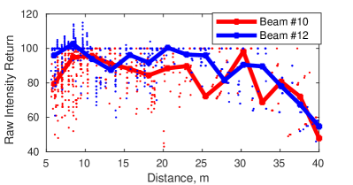
Figure 2: Analysis of raw 8-bit intensity return of 2 beams on the VLP-16, pointing to a uniform high reflectance surface at incidence angle close to zero at different distances. Solid lines are fitted average from raw data. The measurements are noisy, different across beams, and degenerate at large distances.

Therefore, we discard measurements beyond a distance threshold at $30\ m$, and calibrate the remaining using an unsupervised Bayesian approach proposed by Levinson and Thrun [16], as it does not require incidence angle computation and deals with discrete intensity returns directly. The calibration method leads to a mapping function $g_{l}$ for every beam $l$ between a discrete measurement $I_{measured}$ and the most likely true intensity of the surface $I_{true}$:

$$I_{true}=g_{l}(I_{measured})$$ (1)

Finally, we rescale the intensity value to $[0,1]$, where an original value of 100 and beyond is mapped to 1. This is due to very unlikely encounters of retro-reflective objects in the wild and to avoid further firmware correction from the sensor.

III-B Constructing ISHOT

Mathematically, a multi-cue keypoint descriptor $D$, such as ColorSHOT [9], is a chain of generalized Signatures of Histograms $SH^{i}_{(G,f)}(P)$ for the support region around feature point $P$. $G$ is a vector-valued point-wise property of a vertex, and $f$, the metric used to compare two of such point-wise properties.

$$D(P)=\bigcup^{m}_{i=1}SH^{i}_{(G,f)}(P)$$ (2)

Here, $m$ denotes the number of different data cues. Inspired by ColorSHOT [9], we use two types of cues $m=2$, consisting of a geometric component Signature of Histograms of OrienTations SHOT [12] and a texture component using calibrated intensity returns. Our matching metric $f$ is the difference between each sample inside the support region $Q$ and the feature point $P$:

$$f(I_{P},I_{Q})=I_{P}-I_{Q}$$ (3)

The histogram of intensity differences is configured to have 31 bins in each of the 32 spatial support regions inside a keypoint’s neighborhood. The definition of the support regions are identical to the original formulation from SHOT [12]. Together with the 352 dimensions of the original SHOT descriptor, ISHOT has 1344 feature dimensions in our configuration.

Figure 3: Intensity augmented 3D place recognition system overview. A scan is generated by two full rotation of the tilted LiDAR sensor. Keypoints are first detected by ISS-BR in current 3D scan. A batch of ISHOT descriptors are extracted to be matched against the global database, voting for the most likely place candidate. Once match probability passes a threshold, the system proceeds to the geometric consistency refinement stage between scan and database candidates.

IV Probabilistic keypoint voting

We developed our approach based on the keypoint voting pipeline from Bosse and Zlot [10]; however employing our ISHOT 3D local descriptors with the Intrinsic Signature Shapes with Boundary Removal (ISS-BR) [25] keypoint detection. This keypoint sampling technique leads to better matching performance [1] but results into environment-specific keypoint densities. To address this uneven keypoint distribution and leverage the efficacy of ISHOT, we further propose a probabilistic voting approach that updates probabilities of correct place matches by modeling the closest neighbor match voting accuracy in a known environment.

IV-A Place Recognition Pipeline Overview

Our place recognition system (Fig. 3) is based on descriptor matching and place voting. Inputs to our system are local 3D scans and a global feature map discretized into places with the aim to localize the local scan within the global map. A scan consists of all LiDAR measurements accumulated during two full rotations of the actuated sensor, while the vehicle remains stationary. Every individual point is timestamped and projected into the vehicle’s frame based on the motor encoder’s reading at the given timestamp. We first extract ISHOT descriptors from the calibrated local 3D LiDAR scan and then match them against descriptors from places of the global map, voting for the most probable place. After narrowing the search to candidate places within the global map, we perform 3D feature matching between the scan and the candidate places to refine our estimation. The resulting candidate matches are registered using Iterative Closest Point (ICP) to obtain the final transformation between robot and map.

IV-B Global Places Database & Localization Query

A global map is partitioned into discrete places along the trajectory associated (in a SLAM sense) to its creation. The centers of the places are set a minimum distance apart from each other and consist of all measurements within a time window. This distance is set much less then the range of LiDAR detection, so that nearby places overlap. This point cloud is down-sampled by voxelization and the intensity values are corrected with a mapping function and averaged over each voxel. The ISS-BR detector is then used to detect keypoints on the downsampled point cloud of each place. In the last step all keypoints are described using ISHOT, serialized and saved in a database of global places for later retrieval.

When localization is requested, the robot captures a local 3D LiDAR scan of the environment. The local point cloud is then processed similarly to the places. Each resulting feature descriptor from the local point cloud is then matched against the global database of descriptors from all places.

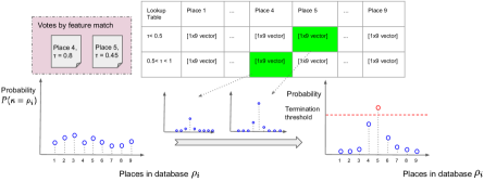
Figure 4: Probability update during a voting process. This example depicts 2 votes from 9 places and 2 $\tau$ ranges. For every vote, a precomputed probability is extracted from the lookup table and merged into the matching probability of places from the database. Instead of voting for one place specifically, a vote updates the probability distribution of all places.

IV-C Probabilistic voting

Our probabilistic voting process considers only the two nearest neighbors for every matched descriptor. The place where the nearest neighbor in the database is extracted from counts as a place candidate $\rho_{v}$, while the Nearest Neighbor Distance Ratio (NNDR) to the second closest match is recorded as a quality measure, similar to the measure presented by Lowe [26]. This NNDR quality measure $\tau$ is defined as follows:

$$\tau=\frac{||\mathbf{d_{q}}-\mathbf{d_{b}}||}{||\mathbf{d_{q}}-\mathbf{d_{b}^{\prime}}||}$$ (4)

where $\mathbf{d_{q}}\in{\mathbf{R}^{1344}}$ denotes the query ISHOT descriptor in scan, $\mathbf{d_{b}}$ and $\mathbf{d_{b}^{\prime}}$ are the closest and second closest neighboring descriptor in the database, respectively. We now define a vote $v$ to consist of a place candidate $\rho_{v}$ and its quality measurement $\tau_{v}$:

$$v=\{\rho_{v},\tau_{v}\}$$ (5)

Assuming each vote is independent, we can update the probability that the current scan $\kappa$ is matched to a place in the database $P(\kappa=\rho_{i})$ given $q$ votes:

$$P(\kappa=\rho_{i})=\eta\cdot\prod_{m=1}^{q}P(\rho_{i}|v_{m})$$ (6)

where $\eta$ is a normalization factor and the probability $P(\rho_{i}|v_{m})$ is precomputed at different $\tau$ and any place $\rho_{i}$ for a given descriptor by modeling the voting precision.

IV-D Modeling voting precision

We model our voting process as a mixed probability distribution, formed from a half-normal and a uniform distribution, dependent on the distance to its real location and matching score $\tau$. The voting process can be modeled as a normal distribution, where places spatially close to ground truth locations are most likely to receive the vote [27], [10]. As we use distances to model this likelihood, we fold the normal distribution to become a half normal distribution with zero mean. The additional uniform distribution accounts for the probability of finding random non-matches and gives the distribution a long tail, as in Fig. 5. Collectively, they form the matching probability of place $\rho_{i}$ given a vote:

$$P(\rho_{i}|d(\rho_{v},\rho_{gt}))=\lambda(\frac{\sqrt{2}}{\sigma\sqrt{\pi}}\exp(\frac{-d(\rho_{v},\rho_{gt})^{2}}{2\sigma^{2}}))+(1-\lambda)$$ (7)

The probability of matching a place $P(\rho_{i})$ is thus dependent on the place’s distance to ground truth $d(\rho_{v},\rho_{gt})$, where $\lambda$ balances the ratio between the two probabilities and $\sigma$ is the variance for the normal distribution. For a given descriptor and a range of $\tau$, the two parameters $\sigma,\lambda$ are found by fitting the theoretical curve of a Cumulative Distribution Function (CDF) to training data matched using ground truth, see Fig. 5.

Figure 5: (upper) Distribution of votes resembles half-normal distribution with a uniformly distributed long tail. The long flat tail up to 400 m is omitted for visibility. Lower $\tau$ ranges correspond to higher matching quality, and appear less frequent. (lower) Fitting parameters for two ranges of $\tau$ using the cumulative distribution function.

IV-E Probability update and terminate condition

To avoid the expensive descriptor computation and matching in a high dimensional space, we leverage the improved quality of our descriptor by only computing and matching them when needed. In every iteration, we compute and match features for a randomly selected subset of unprocessed keypoints, and update the matching probability of all places in the database from the votes. Given the fitted distribution of voting for each $\tau$ range, we precompute a matching probability for every place at every possible vote pair ${\rho_{v},\tau_{v}}$ by approximating the ground truth $\rho_{gt}$ with the current voted place $\rho_{v}$ using (7).

This probability is computed for every place in the database and normalized to sum to 1. It can be interpreted as a confidence metric that determines whether the current vote is coming from a place $i$, given the matching quality $\tau$ and the spatial relationship of places in the database. After the feature matching, for every vote $\{\rho_{v},\tau_{v}\}$ in the batch, a vector is extracted from the table to update the matching probability of place $i$ in the database, see Fig. 4. We apply additional normalization to account for the different keypoint densities within each place in the database. If any candidate has a probability that surpasses a certain threshold $\xi_{v}$, the algorithm proceeds to the geometric verification step directly, skipping the computation and matching of further features. If the given threshold is never reached after all keypoint descriptors are matched, the places are checked by their voting scores.

IV-F Fine registration and geometric consistency check

Once the probability of a place surpasses the acceptance threshold, we roughly align the current scan against the candidate place by matching the local features with features from the place candidate and finding geometric consistent transformations. The matching is simpler as the database only consists of keypoints from one place, but it needs to be run multiple times for multiple candidate places. Here, SHOT is chosen for its much faster matching while preserving relatively high quality feature matching. Starting from this initial estimate, we apply point-to-plane ICP between the voxelized candidate place and current scan for the fine registration, and accept the registration result if the remaining sum of squared distance does not surpass an empirically determined threshold $\epsilon_{ICP}$.

V Experiments

We now evaluate our approach on several real-world datasets. We first introduce the datasets, then present experimental findings for isolated and integrated experiments. We benchmark the proposed ISHOT descriptor against popular geometric descriptors in an Area Under the precision-recall Curve (AUC) evaluation similar to Guo et al. [1]. Finally, we compare the full probabilistic voting pipeline using ISHOT against reference localization approaches.

V-A Datasets

The benchmarking dataset consists of one large map and three sets of LiDAR scans. The datasets were generated outdoors at Queensland Centre for Advanced Technologies (QCAT) in Brisbane, Australia.

The environment was first mapped with a state-of-the-art SLAM algorithm [28] using our autonomous “Gator” platform [29], which is equipped with a rotating 3D LiDAR sensor, as shown in Fig. 3. From the point cloud we generate 438 places, covering an area of approximately 160,000 $m^{2}$. The three sets of scans were generated using the same sensor setup under different conditions from “easy” to “hard”. All scans were collected within $10\ m$ from the original trajectory(see Fig. 6), and processed to include two rotations of encoder.

1. gator dataset: consists of 58 static scans, generated by the mapping vehicle on diverse locations on the map.

2. pole dataset: consists of 41 static scans using the same sensor module on the pole independent from the mobile platform. The pole is held at diverse heights between $0.8\ m$ to $2.5\ m$ around the site to create viewpoint differences. The point clouds are gravity aligned.

3. occlusion dataset: consists of 31 static scans generated by the mobile platform over the complete map. The field of view is partially occluded by buildings, cars, passengers and industrial items.

Ground truth transformations for all datasets with respect to the global map is obtained by manually aligning the point clouds. Additionally, we record a calibration dataset for the intensity calibration of the LiDAR sensor which consists of a 120 seconds driving sequence with the Gator platform on the QCAT site.

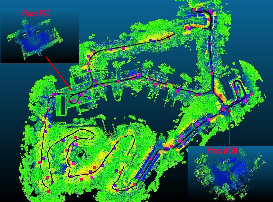
Figure 6: Map of QCAT. Pre-processed map with colors correspond pre-processed intensity value. Black curve is the trajectory during map creation. Squared markers are the ground truth location of where the static scans took place. purple: gator dataset, pink: pole dataset, magenta: occlusion dataset. Two example places are shown in the corner.

V-B Evaluation of local descriptors

Firstly, we calibrate the LiDAR sensor according to Section III on the calibration dataset. Fig. 7 shows the calibration result of all 16 beams on VLP-16.

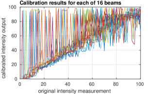
Figure 7: The expected environment intensity given each beam’s intensity return between 0 and 100. All 16 beams are shown here, note there is significant variation between beams.

For evaluating the descriptive power of ISHOT, we use the gator and pole datasets, where individual descriptors are matched against their nearest neighbors in the map descriptor database. We use precision, recall, and AUC as performance measures for this evaluation. True positives are counted if a matched descriptor originates from a place that falls within $5\ m$ of the ground truth location. The results are compared against a range of popular 3D descriptors, including Unique Shape Context (USC) [30], Fast Point Feature Histograms (FPFH)[2], Neighbour-Binary Landmark density Descriptor (NBLD) [11], Gestalt3D [10] and SHOT [12]; see Table I. We vary the $\tau$ ratios as defined in (4) from $0.5$ to $1$ for generation of the performance measures.

TABLE I: Local 3D descriptors used in the evaluation.

descriptor	summary	size
USC	histogram of point distribution	1980
FPFH	histogram of geometric features	33
Gestalt3D	signature of point distribution	130
NBLD	binary signature of point distribution	1408
SHOT	signature of histograms of orientations	352
ISHOT	signature of histograms of orientations and intensity	1344

The ISS-BR keypoint detector salient radius is set to $2.4\,m$. To ensure a fair comparison, we select parameters such that each local descriptor describes a similar volume of the point cloud. For all descriptors, we choose $7\,m$ for the radius and $12\,m$ as the height for structural descriptors (NBLD and Gestalt3D). Furthermore, we discard all measurements over $40\,m$ to ensure sufficient point density and downsample the point clouds using a voxel grid of $0.4\,m$, as recommended by previous work [10]. The average is taken for all intensity measurement inside the voxel. For every descriptor, a database of 154,800 features are generated from the 438 places of the map, against which we match the grand total of 29,342 features extracted from 99 scans, meaning 296 keypoints per scan on average.

(a)

(b)

Figure 8: Local descriptor evaluation results on gator dataset (upper) and the more difficult pole (lower) datasets.

The experimental results are depicted in Fig. 8 and Table II. ISHOT uses raw intensity returns, while ISHOT-C is using calibrated intensity returns. The results illustrate that ISHOT outperforms all benchmarked descriptors significantly with ISS-BR detector, showing the ability to disambiguate places using intensity returns. The intensity calibration increases the descriptiveness further yielding an improvement of 73.85% and 59.35% against the best geometric only descriptor SHOT. Interestingly, ISHOT-C improves the overall recall rate by giving up some precision at low $\tau$, compared to ISHOT. By mapping distinctive measurements to fewer statistically dominant “true” values, calibration indeed helped bringing similar surfaces closer in the descriptor space. Table II also shows averaged processing times for feature description and matching for each scan. This benchmark is timed on Intel i7-4910MQ CPU using Open-source library libNabo [31] for descriptor matching.

TABLE II: AUC and matching time of different descriptors.

descriptor	AUC score		rel. AUC		averaged
	gator	pole	gator	pole	time(s)
USC	0.0071	0.0059	-91.64%	-89.52%	27.477
FPFH	0.0117	0.0135	-86.23%	-76.71%	2.221
Gestalt3D	0.0257	0.0063	-69.74%	-89.13%	1.702
NBLD	0.0545	0.0173	-35.80%	-69.99%	9.522
SHOT	0.0849	0.0578	0%	0%	2.855
ISHOT	0.1454	0.0883	+71.12%	+52.85%	7.570
ISHOT-C	0.1477	0.0921	+73.85%	+59.35%	7.311

V-C Evaluation of place recognition

We evaluate the full probabilistic place recognition algorithm on the gator, pole and occlusion datasets. As performance metric, we measure the success rate of the localization, i.e., the ratio of providing a pose estimation in the global map within 3 meters of manually labeled ground truth location. For comparison, we benchmark our approach against several global localization methods, i.e., global geometric-based registration using SHOT similar to Rusu et al. [2], the original keypoint voting approach with Gestalt3D features [10], and the DELIGHT place recognition approach [6]. In global geometric-based registration, keypoints from local scans are matched against keypoints from global map without discretization into separate places. The latter two approaches are introduced in the previous Section II.

TABLE III: Evaluation of Different Global Localization Pipelines

Pipeline	(a) SHOT global		(b) Gestalt Keypoint Voting		(c) DELIGHT 2-stage wake-up		(d) ISHOT probabilistic voting
Description	success rate	time(s)	success rate	time(s)	success rate	time(s)	success rate	time(s)
gator	53.4%	26.25(4.37)	91.3%	18.47(16.86)	98.1%	5.7(2.1)	100%	8.06(5.45)
pole	65.9%	8.38(3.63)	78.1%	22.35(16.57)	80.5%	10.51(2.72)	92.7%	6.20(3.74)
occlusion	67.7%	22.3(4.29)	74.2%	22.39(21.48)	80.6%	8.67(2.55)	93.5%	7.00(3.77)
overall	60.8 %	19.7	83.1%	20.63	88.4%	7.93	96.1%	7.22

The same geometric verification module is used for all pipelines with a minimum cluster size of 8 and consensus set resolution of $7\ m$. The ICP error threshold $\epsilon_{ICP}$ is chosen at $7\ m^{2}$. The global geometric-based registration matches $K=4$ closest neighboring features in the database to establish keypoint correspondences. Gestalt3D keypoint voting uses a uniform sampling of 10% and matches against $K=10$ closest features, with the voting threshold set to parameters from the original paper [10]. The ISHOT probabilistic voting process has a batch size of 16. The threshold $\xi_{v}$ is chosen empirically at 15%.

By modeling the matching probability and considering the spatial relationship between places, we validate that our probabilistic voting approach can terminate the matching process much earlier than the original voting process, while scoring higher precision. In fact, if the scan originates from industrial areas within the map, the matching is typically terminated after just one batch.

Table III lists the success ratio and the average and median (in parentheses) time spent for different place recognition approaches, using the same hardware as in the previous evaluation. While the Gestalt3D keypoint voting and DELIGHT approaches achieve competitive success rates on all datasets, our approach consistently achieves success rates over 90%, with 100% success rate on the gator dataset. It outperforms the reference algorithms on the more challenging datasets by a margin of over 10%. the processing times are similar to DELIGHT, but slightly faster on average. The median time is often much lower than the average, as few difficult scans require the pipelines to extract and match all features or examine multiple candidates, drastically increase the processing time.

Additionally, we run the pipeline on a challenging driving dataset, and achieve an averaged global localization update rate at 0.25 Hz on same hardware as in Table II. The scene is corrupted by dynamic objects and distorted by vehicle’s motion. We profiled the system’s performance as in Fig. 9. The ISHOT descriptor matching in high-dimensional space is the current bottleneck of the algorithm.

Figure 9: Profiled performance (milliseconds) of our probabilistic keypoint voting place recognition pipeline

VI Discussion & Limitations

Intensity return generates highly reproducible and informative results for a LiDAR sensor. Previous literature in robotics that involve using uncalibrated intensity returns do not report performance across different sensors. The internal pre-processing of measurements by the sensor used in our experiments is unobservable to the user, rendering the localization between different sensors difficult. Velodyne attributes such pre-processing to the need of a clear distinction between retro-reflective and diffusive objects by their customers and the device is not able to provide raw sensor energy return.

We notice a clear need for general LiDAR intensity calibration standards as our results indicate the strong benefits of intensity values in robot localization.

VII Conclusions

We presented ISHOT, a local descriptor combining geometric and texture information of a LiDAR sensor using calibrated LiDAR intensity returns. The descriptor outperforms state-of-art geometric descriptors by a significant margin in real world local descriptor evaluations. We furthermore propose a probabilistic keypoint voting place recognition pipeline and evaluate our work in challenging outdoor experiments. The proposed framework achieves competitive real-time global place recognition performance while being robust to viewpoint changes and occlusion. In the future we aim to find more general procedure to use intensity return across a variety of LiDAR sensors.

References

- [1] Y. Guo, M. Bennamoun, F. Sohel, M. Lu, J. Wan, and N. M. Kwok, “A Comprehensive Performance Evaluation of 3D Local Feature Descriptors,” International Journal of Computer Vision, vol. 116, no. 1, pp. 66–89, Jan. 2016.
- [2] R. B. Rusu, N. Blodow, and M. Beetz, “Fast Point Feature Histograms (FPFH) for 3D registration,” in 2009 IEEE International Conference on Robotics and Automation, May 2009, pp. 3212–3217.
- [3] R. Dubé, D. Dugas, E. Stumm, J. Nieto, R. Siegwart, and C. Cadena, “SegMatch: Segment based place recognition in 3D point clouds,” in 2017 IEEE International Conference on Robotics and Automation (ICRA), May 2017, pp. 5266–5272.
- [4] A. Gawel, C. Del Don, R. Siegwart, J. Nieto, and C. Cadena, “X-View: Graph-Based Semantic Multi-View Localization,” 2017 IEEE Robotics and Automation Letters, Sep. 2017.
- [5] M. A. Uy and G. H. Lee, “PointNetVLAD: Deep Point Cloud Based Retrieval for Large-Scale Place Recognition,” arXiv:1804.03492 [cs], Apr. 2018.
- [6] K. P. Cop, P. V. K. Borges, and R. Dube, “DELIGHT: An Efficient Descriptor for Global Localisation using LiDAR Intensities,” in 2018 IEEE International Conference on Robotics and Automation (ICRA), Brisbane, May 2018, p. 8.
- [7] T. D. Barfoot, C. McManus, S. Anderson, H. Dong, E. Beerepoot, C. H. Tong, P. Furgale, J. D. Gammell, and J. Enright, “Into Darkness: Visual Navigation Based on a Lidar-Intensity-Image Pipeline,” in Robotics Research, ser. Springer Tracts in Advanced Robotics. Springer, Cham, 2016, pp. 487–504.
- [8] J. Neira, J. D. Tardos, J. Horn, and G. Schmidt, “Fusing range and intensity images for mobile robot localization,” IEEE Transactions on Robotics and Automation, vol. 15, no. 1, pp. 76–84, Feb. 1999.
- [9] F. Tombari, S. Salti, and L. D. Stefano, “A combined texture-shape descriptor for enhanced 3D feature matching,” in 2011 18th IEEE International Conference on Image Processing, pp. 809–812.
- [10] M. Bosse and R. Zlot, “Place Recognition Using Keypoint Voting in Large 3D Lidar Datasets,” in 2013 IEEE International Conference on Robotics and Automation (ICRA), May 2013.
- [11] T. Cieslewski, E. Stumm, A. Gawel, M. Bosse, S. Lynen, and R. Siegwart, “Point cloud descriptors for place recognition using sparse visual information,” in 2016 IEEE International Conference on Robotics and Automation (ICRA), May 2016, pp. 4830–4836.
- [12] F. Tombari, S. Salti, and L. D. Stefano, “Unique Signatures of Histograms for Local Surface Description,” in Computer Vision – ECCV 2010, ser. Lecture Notes in Computer Science. Springer, Berlin, Heidelberg, Sep. 2010, pp. 356–369.
- [13] B. Steder, M. Ruhnke, S. Grzonka, and W. Burgard, “Place recognition in 3D scans using a combination of bag of words and point feature based relative pose estimation,” in IEEE International Conference on Intelligent Robots and Systems, Sep. 2011, pp. 1249–1255.
- [14] A. Aldoma, Z. Marton, F. Tombari, W. Wohlkinger, C. Potthast, B. Zeisl, R. B. Rusu, S. Gedikli, and M. Vincze, “Tutorial: Point Cloud Library: Three-Dimensional Object Recognition and 6 DOF Pose Estimation,” IEEE Robotics Automation Magazine, vol. 19, no. 3, pp. 80–91, Sep. 2012.
- [15] J. Collier, S. Se, V. Kotamraju, and P. Jasiobedzki, “Real-Time Lidar-Based Place Recognition Using Distinctive Shape Descriptors,” in Proceedings of SPIE - The International Society for Optical Engineering, vol. 8387, Apr. 2012.
- [16] J. Levinson and S. Thrun, “Unsupervised Calibration for Multi-beam Lasers,” in Experimental Robotics, ser. Springer Tracts in Advanced Robotics. Springer, Berlin, Heidelberg, 2014, pp. 179–193.
- [17] B. Steder, M. Ruhnke, R. Kümmerle, and W. Burgard, “Maximum likelihood remission calibration for groups of heterogeneous laser scanners,” in 2015 IEEE International Conference on Robotics and Automation (ICRA), May 2015, pp. 2078–2083.
- [18] A. Hata and D. Wolf, “Road marking detection using LIDAR reflective intensity data and its application to vehicle localization,” in 17th International IEEE Conference on Intelligent Transportation Systems (ITSC), Oct. 2014, pp. 584–589.
- [19] J. Castorena and S. Agarwal, “Ground-Edge-Based LIDAR Localization Without a Reflectivity Calibration for Autonomous Driving,” IEEE Robotics and Automation Letters, vol. 3, no. 1, pp. 344–351, Jan. 2018.
- [20] I. A. Barsan, S. Wang, A. Pokrovsky, and R. Urtasun, “Learning to localize using a lidar intensity map,” in Proceedings of The 2nd Conference on Robot Learning, ser. Proceedings of Machine Learning Research, A. Billard, A. Dragan, J. Peters, and J. Morimoto, Eds., vol. 87. PMLR, 29–31 Oct 2018, pp. 605–616. [Online]. Available: http://proceedings.mlr.press/v87/barsan18a.html
- [21] M. S. Khan, “3D Robotic Mapping and Place Recognition,” Dissertation, 2017.
- [22] S. Kohlbrecher, J. Meyer, T. Graber, K. Petersen, U. Klingauf, and O. von Stryk, “Hector open source modules for autonomous mapping and navigation with rescue robots,” in RoboCup, 2013.
- [23] S. Lynen, T. Sattler, M. Bosse, J. A. Hesch, M. Pollefeys, and R. Y. Siegwart, “Get Out of My Lab: Large-scale, Real-Time Visual-Inertial Localization,” in Robotics: Science and Systems XI. RSS, 2015, p. 37.
- [24] J. Wolfgang, “Velodyne Software Version V2.0,” https://velodynelidar.com/docs/datasheet/63-9229_Rev-H_Puck%20_Datasheet_Web.pdf, Dec. 2012, accessed: 2018-09-30.
- [25] Y. Zhong, “Intrinsic shape signatures: A shape descriptor for 3D object recognition,” in 2009 IEEE 12th International Conference on Computer Vision Workshops, ICCV Workshops, pp. 689–696.
- [26] D. G. Lowe, “Distinctive image features from scale-invariant keypoints,” International Journal of Computer Vision, vol. 60, no. 2, pp. 91–110, Nov 2004.
- [27] M. Gehrig, E. Stumm, T. Hinzmann, and R. Siegwart, “Visual Place Recognition with Probabilistic Vertex Voting,” in 2017 IEEE International Conference on Robotics and Automation (ICRA), Oct. 2017.
- [28] M. Bosse and R. Zlot, “Continuous 3D scan-matching with a spinning 2D laser,” in IEEE International Conference on Robotics and Automation (ICRA), Kobe, Jun. 2009, pp. 4312–4319.
- [29] A. R. Romero, P. V. K. Borges, A. Elfes, and A. Pfrunder, “Environment-aware sensor fusion for obstacle detection,” in 2016 IEEE International Conference on Multisensor Fusion and Integration for Intelligent Systems (MFI), Sep. 2016, pp. 114–121.
- [30] F. Tombari, S. Salti, and L. Di Stefano, “Unique shape context for 3d data description,” in Proceedings of the ACM Workshop on 3D Object Retrieval - 3DOR ’10. Firenze, Italy: ACM Press, 2010, p. 57.
- [31] J. Elseberg, S. Magnenat, R. Siegwart, and A. Nuchter, “Comparison on nearest-neigbour-search strategies and implementations for efficient shape registration,” Journal of Software Engineering for Robotics (JOSER), vol. 3, pp. 2–12, Jan. 2012.