Two-sample Test of Community Memberships of Weighted Stochastic Block Models

Abstract

Suppose two networks are observed for the same set of nodes, where each network is assumed to be generated from a weighted stochastic block model. This paper considers the problem of testing whether the community memberships of the two networks are the same. A test statistic based on singular subspace distance is developed. Under the weighted stochastic block models with dense graphs, the limiting distribution of the proposed test statistic is developed. Simulation results show that the test has correct empirical type 1 errors under the dense graphs. The test also behaves as expected in empirical power, showing gradual changes when the intra-block and inter-block distributions are close and achieving 1 when the two distributions are not so close, where the closeness of the two distributions is characterized by Renyi divergence of order 1/2. The Enron email networks are used to demonstrate the proposed test.

journalname

and t1This research was supported in part by the National Institutes of Health Grants GM123056 and GM129781.

1 Introduction

Network data appear in many disciplines such as social science, neuroscience, and genetics. Many models have been proposed for network data, among which the stochastic block models (SBMs) (Holland, Laskey and Leinhardt, 1983) have emerged as a popular statistical framework for modeling network data with community structures. SBMs are a class of generative models for describing the community structure in unweighted networks. The model assigns each of $n$ nodes to one of $K_{n}$ blocks, and each edge exists with a probability specified by the block memberships of their endpoints. To account for edge weights, the observations are given in the form of a weighted adjacency matrix. As extensions of unweighted SBMs, weighted SBMs have been proposed, where the weight of each edge is generated independently from some probability density determined by the community membership of its endpoints (Jog and Loh, 2015a, b; Xu, Jog and Loh, 2017).

Alternative to SBMs, random dot product graph (RDPG) models have been proposed where the adjacency matrix of the nodes is generated from Bernoulli distributions with probabilities defined through latent positions. The latent positions can be random and generated from some distribution. Such RDPG models are related to stochastic block model graphs and degree-corrected stochastic block model graphs (Karrer and Newman, 2011), as well as mixed membership block models (Airoldi et al., 2008).

Community identification in a network is an important problem in network data analysis. Spectral clustering is one of the mostly studied methods for community identification based on SBMs (Von Luxburg, Belkin and Bousquet, 2008; Rohe et al., 2011; Mossel, Neeman and Sly, 2012; McSherry, 2001; Lei et al., 2015, 2016; Zhang et al., 2016; Joseph et al., 2016; Schiebinger et al., 2015). Lei et al. (2015) showed that, under mild conditions, spectral clustering applied to the adjacency matrix of the network can consistently recover the hidden communities even when the order of the maximum expected degree is as small as $\log n$ where $n$ is the number of nodes. Xu, Jog and Loh (2017); Jog and Loh (2015a) established the optimal rates for community estimation in the weighted SBMs. Lei et al. (2016); Bickel and Sarkar (2016) developed goodness of fit tests on number of clusters ${K}$ for SBMs.

This paper considers the problem of two-sample inference in the setting that two networks are observed for the same set of nodes, where each network is assumed to be generated from a weighted SBM. We specifically consider the problem of testing whether the community memberships of the two networks are the same. Such tests have many applications. For example, one might be interested in testing whether there is a change of community structures over time and whether a set of genes have different network structures between disease and normal states. This problem has not been studied in literature for weighted SBMs. There are some related inference works developed for the RDPGs (Athreya et al., 2018), but these methods do not treat the block memberships as the parameters of interest. Tang et al. (2017a, b) considered the problem of testing whether two independent finite-dimensional random dot product graphs have the same generating latent positions or the respective generating latent positions are scaled or diagonal transformations of each other. Cape, Tang and Priebe (2017); Athreya et al. (2016); Tang et al. (2018); Cape, Tang and Priebe (2018); Tang et al. (2017b, a) extend the discussion on an interesting asymptotic expansion of subspace distance in Frobenius norm and considered the two-sample test problem by upper bounds of subspace distance (or its variants), but the limiting distribution for test statistic is unknown (Tang et al., 2017a, b).

Ghoshdastidar and von Luxburg (2018) and Ghoshdastidar et al. (2017) considered a different two-sample hypothesis testing problem, where one observes two random graphs, possibly of different sizes. Based on the two given network graphs, they are interested in testing whether the underlying distributions that generate the graphs are same or different. Their proposed test statistic is based on some summary statistics associated with the graphs.

Based on singular subspace distance in Frobenius norm, this paper derives a test statistic of two-sample community memberships of weighted stochastic block models. Different from the previous two-sample test statistics of Tang et al. (2017a, b), we derive the limiting distribution of our proposed test statistic by moment matching method using random matrix theory for Gaussian ensembles. Such results have not appeared in literature even for the dense graphs. A recent independent work of Bao, Ding and Wang (2018) derived the normal distribution for singular subspace in Frobenius for low-rank matrices with Wigner noises. The major difficulty to overcome is to prove that the asymptotic expansion in Tang et al. (2017a, b) still holds in the dense graph region in order to derive mean and variance of our test statistic (4.4) (see Theorem 4 in Section 5).

The rest of the paper is organized as follows. Section 2 defines the homogeneous weighted SBMs and the conditions for dense graphs. Section 4 presents the statistical definition of the null hypothesis that two networks have the same community structures and presents our proposed test statistic. Section 5 presents its limiting distribution. Simulation results to evaluate the type I errors and the power of the proposed test are given in Section 6. Section 7 demonstrates the application of the proposed test to the Enron email networks. Finally, Section 8 gives a brief discussion. Detailed proofs can be found in the Supplemental Materials.

2 Homogeneous weighted SBM and dense graph

2.1 Homogeneous weighted SBM

Homogeneous weighted SBM of $n$ nodes with ${K}$ underlying clusters is characterized by two set of parameters: the underlying membership assignments $\mathbb{Z}_{n}\in\{0,1\}^{n\times{K}}$ and the intra-, inter-edge distributions ${\cal P}_{n},{\cal Q}_{n}$ (Xu, Jog and Loh, 2017; Lei et al., 2016). For the sake of simplicity and similar to Tang et al. (2018), this paper assumes that ${K}$ is fixed.

The underlying membership assignments of a weighted SBM is characterized by $\mathbb{Z}_{n}$ where each row of $\mathbb{Z}_{n}\in\{0,1\}^{n\times{K}}$ contains exactly one $1$, and each column represents the assignments of a particular membership. Here $\mathbb{Z}_{n}$ is treated as fixed parameters for the model. Membership assignments can also be characterized by introducing a mapping function $\mathcal{K}$ (Jog and Loh, 2015b), defined as

Definition 2.1.

Function $\mathcal{K}:[n]\to\left[{K}\right]$ outputs the true membership assignment of each node $i$.

Similar to Gao et al. (2017); Xu, Jog and Loh (2017), we make the following assumption on the size of each block:

Assumption 1 (Size of each block).

There exists $\beta\geq 1$ such that $\frac{n}{\beta{K}}\leq\#\mathcal{C}_{i}\leq\frac{\beta n}{{K}}$ for all $i\in[{K}]$, which implies that $\#\mathcal{C}_{i}\asymp\frac{n}{{K}}$ for all $i\in[{K}]$.

For the sake of simplicity of arguments in proofs, this paper considers that number of clusters $K$ is fixed and makes the following homogeneity assumption on the intra-block, inter-block edge distributions:

Assumption 2 (Homogeneity).

The edge weight probability distributions ${\cal P}_{n},{\cal Q}_{n}$ are supported on $S\subset{\rm I\!R}^{1}$, where $S$ may be $[0,1]$, $[0,\infty)$ or ${\rm I\!R}^{1}$. For $i\leq j\in[n]$,

$$w_{ij}\sim\left\{\begin{array}[]{cc}0,&i=j;\\ {\cal P}_{n},&\mathcal{K}(i)=\mathcal{K}(j),i<j;\\ {\cal Q}_{n},&\mathcal{K}(i)\neq\mathcal{K}(j).\end{array}\right.$$

where $b_{{\cal P}},\sigma_{{\cal P}}^{2}$ are mean and variance of intra-block distribution ${\cal P}_{n}$ and $b_{{\cal P}},\sigma_{{\cal Q}}^{2}$ are mean and variance of inter-block distribution ${\cal Q}_{n}$;. We assume that $\sigma_{{\cal P}}^{2}\asymp b_{{\cal Q}}$, $\sigma_{{\cal Q}}^{2}\asymp b_{{\cal Q}}$, where ${\cal P},{\cal Q}$ are symbols for intra-block and inter-block distributions, not the parameters (Xu, Jog and Loh, 2017). While subscripts $~{}_{n},~{}_{(n)}$ emphasize the dependency on $n$, we ignore these subscripts in $b_{{\cal P}},b_{{\cal Q}},\sigma_{{\cal P}}^{2},\sigma_{{\cal Q}}^{2}$ for the sake of simplicity.

As an example, consider the unweighted SBM $\mathcal{G}_{{K}}\left(p_{n},q_{n}\right)$, we have the adjacency matrix with entity $w_{ij},(i\leq j)$

$$w_{ij}\sim\left\{\begin{array}[]{lc}0,&i=j;\\ {\cal P}_{n}=\text{Bernoulli}\left(p_{n}\right),&\mathcal{K}(i)=\mathcal{K}(j),i<j;\\ {\cal Q}_{n}=\text{Bernoulli}\left(q_{n}\right),&\mathcal{K}(i)\neq\mathcal{K}(j).\end{array}\right.$$

namely, for all $\mathbb{A}_{n}\in\{0,1\}^{n\times n}$ such that $\mathbb{A}_{n}^{T}=\mathbb{A}_{n},a_{ii}=0,i=1,\ldots,n$, the probability

$$\mathbb{P}\left({\mathbb{W}}_{n}=\mathbb{A}_{n}\right)=\prod_{i=1}^{n-1}\left[\prod_{\begin{subarray}{c}j:j>i\\ \mathcal{K}(j)=\mathcal{K}(i)\end{subarray}}p_{n}^{A_{ij}}\left(1-p_{n}\right)^{1-A_{ij}}\cdot\prod_{\begin{subarray}{c}j:j>i\\ \mathcal{K}(j)\neq\mathcal{K}(i)\end{subarray}}q_{n}^{A_{ij}}\left(1-q_{n}\right)^{1-A_{ij}}\right].$$

In this case, Assumption 2 holds with means $b_{{\cal P}}=p_{n},b_{{\cal Q}}=q_{n}$, variances $\sigma_{{\cal P}}^{2}=p_{n}\left(1-p_{n}\right),\sigma_{{\cal Q}}^{2}=q_{n}\left(1-q_{n}\right)$.

For a given network, we observe a symmetric weight matrix ${\mathbb{W}}_{n}\in{\rm I\!R}^{n\times n}=(w_{ij})_{n\times n}$. For all $i<j\in[n]$ the entry $w_{ij}$ are generated independently according to $w_{ij}\sim\mathcal{B}_{\mathcal{K}(i)\mathcal{K}(j),(n)}$. The expectation of the weight matrix ${\mathbb{W}}_{n}$ is

$$\mathbb{E}_{n}\triangleq{\mathbf{E}}{\mathbb{W}}_{n}=\mathbb{Z}_{n}\mathbb{B}_{(n)}\mathbb{Z}_{n}^{T}-{\rm diag}\left(\mathbb{Z}_{n}\mathbb{B}_{(n)}\mathbb{Z}_{n}^{T}\right)\in{\rm I\!R}^{n\times n},$$ (2.1)

where the symmetric matrix $\mathbb{B}_{(n)}=\left(b_{{\cal P}}-b_{{\cal Q}}\right)\mathbb{I}_{{K}}+b_{{\cal Q}}{\bf 1}_{{K}}{\bf 1}_{{K}}^{T}\in{\rm I\!R}_{\geq 0}^{{K}\times{K}}$ represents expectation of intra-block and inter-block distributions and ${\rm diag}({\mathbb{M}})={\rm diag}\{m_{11},\ldots,m_{ss}\}$ represents a diagonal matrix consisting of diagonal entries of ${\mathbb{M}}\in{\rm I\!R}^{s\times s}$.

2.2 SBMs with dense graphs

This paper focuses on SBMs with dense graphs and with the assumption on signal-to-noise ratio defined by Renyi divergence. As for sparsity of the graph, sparsity factor is analogous to Tang et al. (2017b, 2018). The Renyi divergence and the dense graphs are assumed to satisfy Assumption 3:

Assumption 3 (Region of interest).

$$b_{{\cal P}}>b_{{\cal Q}}\gtrsim{s_{n}},\frac{n{{\mathbf{I}}_{\text{Renyi}}^{\frac{1}{2}}}\left({\cal P}_{n}\|{\cal Q}_{n}\right)}{{K}\log n}\gtrsim 1,$$ (2.2)

where ${s_{n}}=n^{-\frac{1}{2}+\epsilon}$ is the asymptotic lower bound for graph sparsity for some $\epsilon>0$, and the Renyi divergence of order $\frac{1}{2}$ is defined as

$${{\mathbf{I}}_{\text{Renyi}}^{\frac{1}{2}}}\left({\cal P}_{n},{\cal Q}_{n}\right)\triangleq-2\log\int\left(\frac{d{\cal P}_{n}}{d{\cal Q}_{n}}\right)^{\frac{1}{2}}d{\cal Q}_{n},$$

where the lower threshold for Renyi divergence might not be tight.

It is worth noting that sparsity factor threshold is consistent with Tang, Cape and Priebe (2017). For unweighted SBMs, Lemma B.1 in Zhang et al. (2016) provides relation between Renyi divergence of order $\frac{1}{2}$ and SNR, and Assumption 3 reduces to

$$p_{n}>q_{n}\gtrsim{s_{n}},SNR\triangleq\frac{(p_{n}-q_{n})^{2}}{p_{n}}\gtrsim\frac{{K}\log n}{n},$$ (2.3)

where the SNR is the signal-to-noise ratio frequently discussed in the literature of community recovery in SBM Abbe (2017); Athreya et al. (2018). Our SNR refers to summary table of exact recovery on page 18 of Abbe (2017).

3 Procrustes Transformation and Property of Singular Subspace Distance for One Network

Since the spectral clustering is used to identify the community memberships of the nodes of the two SBMs, we first provide Definition 3.1:

Definition 3.1.

For a symmetric $n\times n$ matrix ${\mathbb{G}}_{n}$, singular value decomposition is denoted as

$${\mathbb{G}}_{n}=\sum_{i=1}^{n}\lambda_{i}{\mathbf{v}}_{i}{\mathbf{v}}_{i}^{T}=\mathbb{V}_{{\mathbb{G}}_{n}}{\Lambda}_{{\mathbb{G}}_{n}}\mathbb{V}_{{\mathbb{G}}_{n}}^{T}+\mathbb{V}_{{\mathbb{G}}_{n}}^{\perp}{\Lambda}_{{\mathbb{G}}_{n}}^{\perp}\left(\mathbb{V}_{{\mathbb{G}}_{n}}^{\perp}\right)^{T},|\lambda_{1}|\geq\ldots\geq|\lambda_{n}|,$$ (3.1)

where ${\Lambda}_{{\mathbb{G}}_{n}}={\rm diag}\left\{\lambda_{1},\ldots,\lambda_{{K}}\right\}$ contains leading ${K}$ singular components of ${\mathbb{G}}_{n}$ while ${\Lambda}_{{\mathbb{G}}_{n}}^{\perp}$ contains the rest. $\mathbb{V}_{{\mathbb{G}}_{n}}\in{\rm I\!R}^{n\times{K}}$ may not be unique (due to multiple root) but just pick one collection.

In this paper, the singular value decomposition is applied to the observed connection matrix ${\mathbb{G}}_{n}$=${\mathbb{W}}_{n}$ or its expected values ${\mathbb{G}}_{n}=\mathbb{E}_{n}$ (Tang et al., 2017b, 2018).

To begin with, we define the orthogonal Procrustes transformation from matrix $\mathbb{V}_{1}\in{\rm I\!R}^{n\times{K}}$ to $\mathbb{V}_{2}\in{\rm I\!R}^{n\times{K}}$:

$${{\cal P}\mathcal{T}}\left(\mathbb{V}_{1},\mathbb{V}_{2}\right)\in\arg\inf_{\mathbb{U}\in{\cal O}({K})}\left\|\mathbb{V}_{1}\mathbb{U}-\mathbb{V}_{2}\right\|_{F}\subset{\rm I\!R}^{{K}\times{K}},$$ (3.2)

where we do not need to specify the relationship between ${{\cal P}\mathcal{T}}\left(\mathbb{V}_{1},\mathbb{V}_{2}\right)$ and ${{\cal P}\mathcal{T}}\left(\mathbb{V}_{2},\mathbb{V}_{1}\right)$. We further define

$$\left\|\sin\Theta\left(\mathbb{V}_{1},\mathbb{V}_{2}\right)\right\|_{F}\triangleq\left\|\mathbb{V}_{1}{{\cal P}\mathcal{T}}\left(\mathbb{V}_{1},\mathbb{V}_{2}\right)-\mathbb{V}_{2}\right\|_{F}$$ (3.3)

as the $\sin\Theta$ distance in Frobenius norm.

We first establish the distance between singular vectors of $\mathbb{V}_{{\mathbb{W}}_{n}}$ and $\mathbb{V}_{\mathbb{E}_{n}}$ after the Procrustes transformation $\mathbb{T}$. One natural definition is the Frobenius norm of two matrices $\left\|\mathbb{V}_{{\mathbb{W}}_{n}}\mathbb{T}-\mathbb{V}_{\mathbb{E}_{n}}\right\|_{F}$. However, the mean and variance of this distance is complicated; details of this argument can be found in Appendix E. Instead, we consider a modified and re-scaled quantity defined as

$$\left\|\left(\mathbb{V}_{{\mathbb{W}}_{n}}\mathbb{T}-\mathbb{V}_{\mathbb{E}_{n}}\right){\Lambda}_{\mathbb{E}_{n}}\right\|_{F},$$

which has a simpler mean and variance. We have the following asymptotic expansion for the singular value decompositions of the SBMs:

Lemma 1.

$$\frac{1}{\sqrt{{K}nb_{{\cal P}}}}\left\|\left(\mathbb{V}_{{\mathbb{W}}_{n}}\mathbb{T}_{n}-\mathbb{V}_{\mathbb{E}_{n}}\right){\Lambda}_{\mathbb{E}_{n}}\right\|_{F}$$

$$= \frac{1}{\sqrt{{K}nb_{{\cal P}}}}\left\|\left({\mathbb{W}}_{n}-\mathbb{E}_{n}\right)\mathbb{V}_{\mathbb{E}_{n}}\right\|_{F}+O_{P}\left(\sqrt{\frac{{K}}{nb_{{\cal P}}}}\log(n)\right)=O_{P}(1),$$

where transformation matrix $\mathbb{T}$ is Procrustes transformation ${{\cal P}\mathcal{T}}\left(\mathbb{V}_{{\mathbb{W}}_{n}},\mathbb{V}_{\mathbb{E}_{n}}\right)$.

We provide a proof of this Lemma 1 in section C.1 using the same technique as Theorem 2.1 of Tang et al. (2018). Lemma 1 implies

$$\frac{1}{{K}nb_{{\cal P}}}\left\|\left(\mathbb{V}_{{\mathbb{W}}_{n}}\mathbb{T}_{n}-\mathbb{V}_{\mathbb{E}_{n}}\right){\Lambda}_{\mathbb{E}_{n}}\right\|_{F}^{2}=O_{P}(1)$$

$$= \frac{1}{{K}nb_{{\cal P}}}\left\|\left({\mathbb{W}}_{n}-\mathbb{E}_{n}\right)\mathbb{V}_{\mathbb{E}_{n}}\right\|_{F}^{2}$$

$$+\frac{\left\|\left({\mathbb{W}}_{n}-\mathbb{E}_{n}\right)\mathbb{V}_{\mathbb{E}_{n}}\right\|_{F}}{\sqrt{{K}nb_{{\cal P}}}}\cdot O_{P}\left(\sqrt{\frac{{K}}{nb_{{\cal P}}}}\log(n)\right)+O_{P}\left(\frac{{K}\left[\log(n)\right]^{2}}{nb_{{\cal P}}}\right).$$

Theorem 2 shows that the second term in the above asymptotic expansion can be removed.

Theorem 2.

Under the Assumptions 1, 2, 3, we have

$$\frac{1}{{K}n}\left\|\left(\mathbb{V}_{{\mathbb{W}}_{n}}\mathbb{T}-\mathbb{V}_{\mathbb{E}_{n}}\right){\Lambda}_{\mathbb{E}_{n}}\right\|_{F}^{2} = \frac{1}{{K}n}\left\|\left({\mathbb{W}}_{n}-\mathbb{E}_{n}\right)\mathbb{V}_{\mathbb{E}_{n}}\right\|_{F}^{2}+O_{P}\left(\frac{{K}[\log(n)]^{2}}{n}\right),$$

where transformation matrix $\mathbb{T}_{n}$ is Procrustes transformation ${{\cal P}\mathcal{T}}\left(\mathbb{V}_{{\mathbb{W}}_{n}},\mathbb{V}_{\mathbb{E}_{n}}\right)$, we remove $b_{{\cal P}}$ in the denominator in order to be consistent with later test statistic (4.4) in two-sample problem (4.3); we have

$$\frac{1}{{K}n}\left\|\left(\mathbb{V}_{{\mathbb{W}}_{n}}\mathbb{T}_{n}-\mathbb{V}_{\mathbb{E}_{n}}\right){\Lambda}_{\mathbb{E}_{n}}\right\|_{F}^{2}=\Theta_{P}\left(\sigma_{{\cal Q}}^{2}+\frac{\sigma_{{\cal P}}^{2}-\sigma_{{\cal Q}}^{2}}{{K}}\right).$$

Consequentially, variance of the linear representation dominates as well:

$${\rm Var}\left[\frac{1}{{K}n}\left\|\left(\mathbb{V}_{{\mathbb{W}}_{n}}\mathbb{T}_{n}-\mathbb{V}_{\mathbb{E}_{n}}\right){\Lambda}_{\mathbb{E}_{n}}\right\|_{F}^{2}\right]=O\left(\frac{b_{{\cal Q}}^{2}}{nK}\right)$$

$$= {\rm Var}\left[\frac{1}{{K}n}\left\|\left({\mathbb{W}}_{n}-\mathbb{E}_{n}\right)\mathbb{V}_{\mathbb{E}_{n}}\right\|_{F}^{2}\right]+O\left(\frac{{K}^{2}[\log(n)]^{4}}{n^{2}}\right).$$

This asymptotic expansion lead to the limiting distribution of $\frac{1}{{K}n}\left\|\left(\mathbb{V}_{{\mathbb{W}}}\mathbb{T}_{n}-\mathbb{V}_{\mathbb{E}}\right){\Lambda}_{\mathbb{E}}\right\|_{F}^{2}$ as stated in the the following Theorem.

Theorem 3.

Under the assumption 1, 2, 3, we have

$$\frac{\frac{1}{{K}n}\left\|\left(\mathbb{V}_{{\mathbb{W}}_{n}}\mathbb{T}_{n}-\mathbb{V}_{\mathbb{E}_{n}}\right){\Lambda}_{\mathbb{E}_{n}}\right\|_{F}^{2}-\widetilde{\mu}_{n}}{\sqrt{\widetilde{{\rm Var}_{n}}}}\to{\cal N}(0,1),$$ (3.5)

where transformation matrix $\mathbb{T}_{n}$ is Procrustes transformation ${{\cal P}\mathcal{T}}\left(\mathbb{V}_{{\mathbb{W}}_{n}},\mathbb{V}_{\mathbb{E}_{n}}\right)$; the mean is $\widetilde{\mu}_{n}=\sigma_{{\cal Q}}^{2}+\frac{\sigma_{{\cal P}}^{2}-\sigma_{{\cal Q}}^{2}}{{K}}$ and the variance is

$$\widetilde{{\rm Var}_{n}}=\frac{2}{n{K}}\left(\sigma_{{\cal Q}}^{4}+\frac{\sigma_{{\cal P}}^{4}-\sigma_{{\cal Q}}^{4}}{{K}}\right)+O\left(\frac{{K}^{2}[\log(n)]^{4}}{n^{2}}\right).$$

We use symbols $\widetilde{\mu}_{n}$, $\widetilde{{\rm Var}_{n}}$ just because symbols $\mu_{n}$, ${\rm Var}_{n}$ are reserved for the mean of variance of our test statistic $T_{n,{K}}$ (4.4) in Theorem 4.

4 Two-sample Hypothesis Test of Community Memberships Based on SBMs

4.1 A two-sample test problem

Consider the setting where we have two independent networks with the same group of $n$ nodes and each is generated from a weighted SBM with underlying membership assignment $\mathbb{Z}_{n}^{(v)},v=1,2$. We are interested in testing whether underlying block assignments are the same; in other words, testing

$$H_{0}:\mathbb{Z}_{n}^{(1)}\upVdash\mathbb{Z}_{n}^{(2)}\mbox{ versus }H_{1}:\mathbb{Z}_{n}^{(1)}\not\upVdash\mathbb{Z}_{n}^{(2)},$$ (4.1)

where for two matrices ${\mathbb{M}}_{1},{\mathbb{M}}_{2}\in{\rm I\!R}^{n\times{K}}$, ${\mathbb{M}}_{1}\upVdash{\mathbb{M}}_{2}$ means there exists $\mathbb{U}\in{\cal O}({K})$ such that ${\mathbb{M}}_{1}={\mathbb{M}}_{2}\mathbb{U}$ and ${\cal O}({K})$ represents the set of ${K}\times{K}$ orthogonal matrices.

For a weighted SBM, it is known that

$$\mathbb{V}_{\mathbb{E}_{n}}\upVdash\mathbb{Z}_{n}(\mathbb{Z}_{n}^{T}\mathbb{Z}_{n})^{-\frac{1}{2}}.$$ (4.2)

In addition, $\mathbb{Z}_{n}^{(1)}\upVdash\mathbb{Z}_{n}^{(2)}$ if and only if

$$\mathbb{Z}_{n}^{(1)}\left([\mathbb{Z}_{n}^{(1)}]^{T}\mathbb{Z}_{n}^{(1)}\right)^{-\frac{1}{2}}\upVdash\mathbb{Z}_{n}^{(2)}\left([\mathbb{Z}_{n}^{(2)}]^{T}\mathbb{Z}_{n}^{(2)}\right)^{-\frac{1}{2}}.$$

Since an orthogonal matrix is actually a permutation, (4.2) implies that $H_{0}:\mathbb{Z}_{n}^{(1)}\upVdash\mathbb{Z}_{n}^{(2)}$ is equivalent to

$$H_{0}:\mathbb{V}_{\mathbb{E}_{n}^{(1)}}\upVdash\mathbb{V}_{\mathbb{E}_{n}^{(2)}}\mbox{ versus }H_{1}:\mathbb{V}_{\mathbb{E}_{n}^{(1)}}\not\upVdash\mathbb{V}_{\mathbb{E}_{n}^{(2)}}.$$ (4.3)

In order for this null hypothesis to be practically meaningful, we make an additional Assumption 4 on the intra-block and inter-block distributions:

Assumption 4.

For the expectations of intra-block and inter-block distributions stated in Assumption 2), we assume $\mathbb{B}_{(n)}^{(2)}=\gamma\mathbb{B}_{(n)}^{(1)}$, or equivalently, $\gamma=\frac{b_{{\cal P}}^{(1)}}{b_{{\cal P}}^{(2)}}=\frac{b_{{\cal Q}}^{(1)}}{b_{{\cal Q}}^{(2)}}$.

The assumption may seem restrictive. However, if the edge generating functions are different, the underlying network structures will be different and the the null is usually easy to reject.

4.2 Two-sample test statistic

Our proposed test statistic is also based on the Procrustes transformation but we include an ${K}\times{K}$ matrix multiplier ${\Lambda}_{{\mathbb{W}}_{n}^{(2)}}$ in order to simplify the calculations of the mean and variance (see Theorem 16) of the test statistic:

$$T_{n,{K}}=T_{n,{K}}\left(\mathbb{V}_{{\mathbb{W}}_{n}^{(1)}},\mathbb{V}_{{\mathbb{W}}_{n}^{(2)}}\right)\triangleq\frac{1}{n{K}}\left\|\left(\mathbb{V}_{{\mathbb{W}}_{n}^{(1)}}\mathbb{T}_{n}-\mathbb{V}_{{\mathbb{W}}_{n}^{(2)}}\right){\Lambda}_{{\mathbb{W}}_{n}^{(2)}}\right\|_{F}^{2},$$ (4.4)

where $\mathbb{T}_{n}$ is the Procrustes transformation ${{\cal P}\mathcal{T}}\left(\mathbb{V}_{{\mathbb{W}}_{n}^{(1)}},\mathbb{V}_{{\mathbb{W}}_{n}^{(2)}}\right)$.

It is important to point out the difference between our test statistic and the one in Tang et al. (2017a, b). First, our formulation of the null hypothesis test is different from that of RDPGs since RDPGs are parametrized by latent position parameters. Tang et al. (2017a, b) developed a two-sample test on those latent position parameters. Secondly, we provide the limiting distribution of our test statistic by using random matrix theory. In contrast, Tang et al. (2017a, b) proposed to apply bootstrap to the test statistic based on an upper bound estimation.

5 Asymptotic distribution of two-sample test statistic (4.4)

5.1 Asymptotic distribution of the proposed test

Parallel to the results in Theorem 2, we have the following asymptotic expansion for the two-sample test statistic $T_{n,{K}}$:

Theorem 4.

Assume that Assumptions 1, 2, 3, 4 hold. Under the null of (4.3), we have

$$T_{n,{K}} = \frac{1}{{K}n}\left\|\left(\mathbb{V}_{{\mathbb{W}}_{n}^{(1)}}\mathbb{T}_{n}-\mathbb{V}_{{\mathbb{W}}_{n}^{(2)}}\right){\Lambda}_{{\mathbb{W}}_{n}^{(2)}}\right\|_{F}^{2}$$

$$= \frac{1}{{K}n}\left\|\left(\gamma{\mathbb{W}}_{n}^{(1)}-{\mathbb{W}}_{n}^{(2)}\right)\mathbb{V}_{{\mathbb{W}}_{n}^{(2)}}\right\|_{F}^{2}+O_{P}\left(\frac{{K}[\log(n)]^{2}}{n}\right),$$

where transformation matrix $\mathbb{T}_{n}$ is Procrustes transformation ${{\cal P}\mathcal{T}}\left(\mathbb{V}_{{\mathbb{W}}_{n}^{(1)}},\mathbb{V}_{{\mathbb{W}}_{n}^{(2)}}\right)$. As a result, the variance of the asymptotic expansion dominates as well,

$${\rm Var}\left[T_{n,{K}}\right] = {\rm Var}\left[\frac{1}{{K}n}\left\|\left(\gamma{\mathbb{W}}_{n}^{(1)}-{\mathbb{W}}_{n}^{(2)}\right)\mathbb{V}_{{\mathbb{W}}^{(2)}}\right\|_{F}^{2}\right]+O\left(\frac{{K}^{2}[\log(n)]^{4}}{n^{2}}\right)=O\left(\frac{b_{{\cal Q}}^{2}}{nK}\right).$$

This asymptotic expansion leads to the limiting distribution of our test statistic (4.4), as stated in the Theorem 5 below:

Theorem 5.

Under the Assumptions 1, 2, 3, 4, our proposed test statistic (4.4) have the following asymptotic distribution under the null of (4.3),

$$\frac{T_{n,{K}}-\mu_{n}}{\sqrt{{\rm Var}_{n}}}\to{\cal N}(0,1),$$ (5.2)

where the mean is

$$\mu_{n}=\gamma^{2}\sigma_{{\cal Q}}^{2,(1)}+\sigma_{{\cal Q}}^{2,(2)}+\frac{1}{{K}}\left[\gamma\sigma_{{\cal P}}^{2,(1)}+\sigma_{{\cal P}}^{2,(2)}-\left(\gamma^{2}\sigma_{{\cal Q}}^{2,(1)}+\sigma_{{\cal Q}}^{2,(2)}\right)\right],$$

and the variance is

$${\rm Var}_{n} = \frac{2}{n{K}}\left[\left(\gamma^{2}\sigma_{{\cal Q}}^{2,(1)}+\sigma_{{\cal Q}}^{2,(2)}\right)^{2}+\frac{\left(\gamma^{2}\sigma_{{\cal P}}^{2,(1)}+\sigma_{{\cal P}}^{2,(2)}\right)^{2}-\left(\gamma^{2}\sigma_{{\cal Q}}^{2,(1)}+\sigma_{{\cal Q}}^{2,(2)}\right)^{2}}{{K}}\right]$$

$$+O\left(\frac{{K}^{2}[\log(n)]^{4}}{n^{2}}\right).$$

In practice, $\mu_{n}$, ${\rm Var}_{n}$ have to be estimated and their estimates need to be corresponding well-behaved estimators:

Definition 5.1 (Well-behaved estimators).

Define the well-behaved estimators as those that

$$\widehat{\mu_{n}}-\mu_{n}=o_{P}\left(b_{{\cal P}}\right),\widehat{{\rm Var}_{n}}-{\rm Var}_{n}=o_{P}\left(\frac{b_{{\cal P}}^{2}}{n{K}}\right).$$ (5.3)

Such well-behaved estimates can be obtained by plugging well-behaved estimators $\widehat{\gamma^{2}\sigma_{{\cal Q}}^{2,(1)}+\sigma_{{\cal Q}}^{2,(2)}}$, $\widehat{\gamma^{2}\sigma_{{\cal P}}^{2,(1)}+\sigma_{{\cal P}}^{2,(2)}}$ for $\gamma^{2}\sigma_{{\cal Q}}^{2,(1)}+\sigma_{{\cal Q}}^{2,(2)}$, $\gamma^{2}\sigma_{P_{n}}^{2,(1)}+\sigma_{{\cal P}}^{2,(2)}$ (Jog and Loh, 2015a, b; Xu, Jog and Loh, 2017; Mossel, Neeman and Sly, 2012; McSherry, 2001; Tang, Cape and Priebe, 2017). We have the following corollary 6 when estimates of means and variances are used in the test statistic.

Corollary 6.

Suppose that Assumptions 1,, 2, 3, 4 hold, our proposed test statistic (4.4) have the following asymptotic distribution under the null hypothesis of (4.3), we have

$$\frac{T_{n,{K}}-\widehat{\mu_{n}}}{\sqrt{\widehat{{\rm Var}_{n}}}}\to{\cal N}(0,1),$$ (5.4)

where the mean is

$$\widehat{\mu_{n}}=\widehat{\gamma^{2}\sigma_{{\cal Q}}^{2,(1)}+\sigma_{{\cal Q}}^{2,(2)}}+\frac{1}{{K}}\left[\widehat{\gamma\sigma_{{\cal P}}^{2,(1)}+\sigma_{{\cal P}}^{2,(2)}}-\widehat{\gamma^{2}\sigma_{{\cal P}}^{2,(1)}+\sigma_{{\cal Q}}^{2,(2)}}\right],$$

and the variance is

$$\widehat{{\rm Var}_{n}} = \frac{2}{n{K}}\left[\widehat{\gamma\sigma_{{\cal Q}}^{2,(1)}+\sigma_{{\cal Q}}^{2,(2)}}^{2}+\frac{\widehat{\gamma\sigma_{{\cal P}}^{2,(1)}+\sigma_{{\cal P}}^{2,(2)}}^{2}-\widehat{\gamma\sigma_{{\cal Q}}^{2,(1)}+\sigma_{{\cal Q}}^{2,(2)}}^{2}}{{K}}\right]$$

$$+O\left(\frac{{K}^{2}[\log(n)]^{4}}{n^{2}}\right).$$

5.2 Asymptotic power of the proposed test

We evaluate the power of the proposed test by specifying the alternative using the Hamming distance between the community memberships, $\mathbb{Z}_{n}^{(1)}$ and $\mathbb{Z}_{n}^{(2)}$ of $n$ nodes

$$\ell_{n}\left(\mathbb{Z}_{n}^{(1)},\mathbb{Z}_{n}^{(2)}\right)\triangleq\frac{1}{n}\min_{\Pi\in{\cal O}\left({K}\right)}d_{H}\left(\mathbb{Z}_{n}^{(1)},\Pi\circ\mathbb{Z}_{n}^{(2)}\right),$$ (5.5)

where $d_{H}\left(\cdot,\cdot\right)$ denotes the Hamming distance, and ${K}$ is the permutation matrix. We consider the following hypothesis test with $\epsilon^{\prime}>0$:

$$H_{0}^{\prime}:\ell_{n}=0\mbox{ v.s. }H_{1}^{\prime}:\ell_{n}\succeq\frac{{K}}{n^{1-\epsilon^{\prime}}\sqrt{\mu_{n}}},$$ (5.6)

where $\mu_{n}$ appears in Theorem 5. We further assume $\frac{n}{{K}}$ is an integer and $\beta=1$ in Assumption 1. In this simple scenario with equal-size assumption,

$$T_{n,{K}} = \frac{1}{n{K}}\left\|\left[\mathbb{V}_{{\mathbb{W}}_{n}^{(1)}}{{\cal P}\mathcal{T}}\left(\mathbb{V}_{{\mathbb{W}}_{n}^{(1)}},\mathbb{V}_{{\mathbb{W}}_{n}^{(2)}}\right)-\mathbb{V}_{{\mathbb{W}}_{n}^{(2)}}\right]\Lambda_{{\mathbb{W}}_{n}^{(2)}}\right\|_{F}^{2}$$

$$\asymp_{P} \frac{1}{n{K}}\left\|\left[\mathbb{Z}_{n}^{(1)}\left(\left[\mathbb{Z}_{n}^{(1)}\right]^{T}\mathbb{Z}_{n}^{(1)}\right)^{-\frac{1}{2}}{{\cal P}\mathcal{T}}_{\mathbb{Z}}-\mathbb{Z}_{n}^{(2)}\left(\left[\mathbb{Z}_{n}^{(2)}\right]^{T}\mathbb{Z}_{n}^{(2)}\right)^{-\frac{1}{2}}\right]\Lambda_{{\mathbb{W}}_{n}^{(2)}}\right\|_{F}^{2}$$

$$= \frac{1}{n{K}}\left(\sqrt{\frac{{K}}{n}}n\ell_{n}\cdot\frac{nb_{{\cal P}}}{{K}}\right)^{2}=\frac{n^{2}b_{{\cal P}}^{2}\ell_{n}^{2}}{{K}^{2}}\succeq n^{2\epsilon^{\prime}}\mu_{n}\succ\mu_{n},$$

where

$${{\cal P}\mathcal{T}}_{\mathbb{Z}}={{\cal P}\mathcal{T}}\left(\mathbb{Z}_{n}^{(1)}\left(\left[\mathbb{Z}_{n}^{(1)}\right]^{T}\mathbb{Z}_{n}^{(1)}\right)^{-\frac{1}{2}},\mathbb{Z}_{n}^{(2)}\left(\left[\mathbb{Z}_{n}^{(2)}\right]^{T}\mathbb{Z}_{n}^{(2)}\right)^{-\frac{1}{2}}\right).$$

Consequentially, we have the following results on the power of the proposed test:

Theorem 7 (Asymptotic power guarantee).

Assume that Assumptions 1, 2, 3 and 4 hold. In addition, assume that $\frac{n}{{K}}$ is an integer and $\beta=1$ in Assumption 1. Then under the alternative $H_{1}^{\prime}$ of (5.6),

$$T_{n,{K}}\succeq_{P}n^{2\epsilon^{\prime}}\mu_{n}\succ\mu_{n},$$

where $\mu_{n}$ appears in Theorem 5; or equivalently,

$$\frac{T_{n,{K}}-\mu_{n}}{\sqrt{{\rm Var}_{n}}}\succeq_{P}n^{\frac{1}{2}+2\epsilon^{\prime}}\cdot\frac{\mu_{n}\sqrt{{K}}}{b_{{\cal P}}}\succeq n^{\frac{1}{2}+2\epsilon^{\prime}}\sqrt{{K}}.$$

Consequentially, for any two-sided $\alpha$ level test with $q_{\frac{\alpha}{2}}$,$q_{\left(1-\frac{\alpha}{2}\right)}$ the $\frac{\alpha}{2}$-quantile and $\left(1-\frac{\alpha}{2}\right)$-quantile of Gaussian distribution, the probability under the alternative $H_{1}^{\prime}$ of (5.6) satisfies

$${\mathbf{P}}_{H^{\prime}_{1}}\left(q_{\frac{\alpha}{2}}<\frac{T_{n,{K}}-\mu_{n}}{\sqrt{{\rm Var}_{n}}}<q_{\left(1-\frac{\alpha}{2}\right)}\right)\to 1.$$

6 Simulation Studies

6.1 Type I errors

We first evaluate the type I errors of the proposed test. Tables 6.1 show the empirical type I errors of the proposed tests for different families of weighted SBMs based on 4,000 replications.

The first model considers unweighted SBMs with $p_{n}=0.5,q_{n}=0.1$ ($p_{n}\asymp 1$) for different sample sizes $n=500,1000,2000$ and $4000$ and different parameter values of $\lambda=1.5,1.3,1.0,1.8$ and $0.7$. Overall, the typer I errors are under control, except that when the sample size is small and $\lambda=0.7$.

The second model considers a family of weighted SBMs with ${\cal P}_{n}=\chi^{2}(5),{\cal Q}_{n}=\chi^{2}\left(1\right)$. In this case $b_{{\cal P}}\asymp 1$, similar type 1 errors are observed as the unweighted SBMs for different values of $\lambda$ and different sample sizes.

The third model considers the unweighted SBM with $p=1.8n^{-\frac{1}{6}},q=0.36n^{-\frac{1}{6}}$. This problem is more complex: type I error is expected to converge when $n\to\infty$, while sparsity makes the convergence rate slower. Overall, the type I errors are under control.

Table 6.1: Type I error of two sided test with significance level $\alpha=5\%$ on unweighted SBM with $p=0.5,q=0.1,{K}=2,\#\mathcal{C}_{1}=2\#\mathcal{C}_{2}$. Run 4000 times for each data point.

$n$	$\gamma=1.5$	$\gamma=1.3$	$\gamma=1$	$\gamma=0.8$	$\gamma=0.7$
	unweighted SBM with $p=0.5,q=0.1$
500	5.3	5.2	4.7	5.0	9.7
1000	4.9	5.2	4.8	4.8	7.3
2000	4.9	5.5	5.3	5.3	5.6
4000	4.5	5.1	5.2	4.7	6.1
	weighted SBM with ${\cal P}_{n}=\chi^{2}(5),{\cal Q}_{n}=\chi^{2}\left(1\right)$
500	5.3	5.7	4.7	5.2	5.4
1000	5.2	4.6	5.2	5.9	5.0
2000	5.2	4.7	5.4	5.3	5.6
4000	5.2	5.1	5.1	5.0	5.3
	unweighted SBM with $p=1.8n^{-\frac{1}{6}},q=0.36n^{-\frac{1}{6}}$
500	5.0	5.0	4.9	5.3	6.1
1000	5.3	5.4	5.7	6.2	6.5
2000	5.1	5.1	5.3	6.0	6.4
4000	5.0	5.1	5.4	5.7	5.9

6.2 Empirical power

Table 6.2 shows the empirical power for two different models. The first model assumes that $p=0.5,q=0.5-200^{-\frac{1}{3}}=0.329$, which corresponds to a SNR =0.0578. The second model assumed that $p=0.5,q_{n}=p-n^{-\frac{1}{3}}(\geq 0.329)$, which gives a SNR=$2n^{-\frac{2}{3}}$. For each scenario, we fix Hamming distance $\ell_{0}$ and increase number of nodes $n$. As expected, as the Hamming distance $\ell_{0}$ between the two community memberships increases, we observe increased power of our proposed test.

Table 6.2: Empirical power of the test with two-sided $\alpha=5\%$. Two unweighted SBMs with two blocks of equal sizes and $\gamma=1$.

	$\ell_{n}\equiv\ell_{0}$
$\ell_{0}$	0.0%	0.1%	0.2%	0.4%	0.5%	1.0%	1.6%	2.0%	5.0%
$p=0.5,q=0.5-200^{-\frac{1}{3}}=0.329$, $SNR=0.0578$
200	5.7	–	–	–	17.0	43.1	70.7	87.0	100.0
500	4.7	–	27.3	72.5	73.5	93.3	99.8	100.0	100.0
1000	4.8	49.1	95.5	100.0	100.0	100.0	100.0	100.0	100.0
2000	5.3	99.8	100.0	100.0)	100.0	100.0	100.0	100.0	100.0
$p=0.5,q_{n}=p-n^{-\frac{1}{3}}(\geq 0.329)$, $SNR=2n^{-\frac{2}{3}}$
200	5.7	–	–	–	17.0	43.1	70.7	87.0	100.0
500	5.1	–	13.6	31.1	32.9	92.9	97.1	100.0	100.0
1000	5.1	14.2	25.9	70.2	86.6	100.0	100.0	100.0	100.0
2000	5.0	20.4	60.8	99.2	100.0	100.0	100.0	100.0	100.0

7 Real Data Example – Enron Email dataset

Table 7.1: Enron dataset: persons’ names and their positions for selected nodes number.

node number	name	position
4	badeer-r	Director
16	causholli-m	Employee
18	cuilla-m	Manager
32	forney-j	Manager
34	gang-l	Employee
84	motley-m	Director
93	presto-k	Vice President
94	quenet-j	Trader
107	salisbury-h	Employee
110	scholtes-d	Trader
114	schwieger-j	Trader
120	slinger-r	Trader
122	solberg-g	Employee
127	stepenovitch-j	Vice President
128	stokley-c	Employee
132	tholt-j	Vice President
138	ward-k	Employee

To demonstrate the proposed test, we analyzed the Enron email network data (May 7th, 2015 version, https://www.cs.cmu.edu/$\sim$enron/). The dataset includes email communication data of 150 users, mostly were in senior management positions, including CEO (4), manager (8), trader (2), president (2), vice president (16), others (57). For each email, we have information on sender, list of recipients and the email date. The email links were included as long as they were sent to some of the 89 users. To construct the weights, if A sent an email to B and C, both weights for edge (A,B) and edge (A,C) was increased by 1. Since the original Enron email network were directed, we converted it into undirected network by setting the weight $w_{new}^{(v)}(A,B)\leftarrow\min\left\{w_{old}^{(v)}(A,B)+w_{old}^{(v)}(B,C),127\right\}$.

There were a total of 11539 emails communications (without self-loops) among the 150 users between 1998 and 2001, represented by a directed graph with maximal weight $\max_{A,B}w_{old}^{all}(A,B)=361$. We performed spectral clustering analysis based on the Laplacian of the weight matrix $\mathcal{L}\left({\mathbb{W}}_{n}^{(v)}\right)$ and applied k-means clustering methods. Similar to Xu and Hero III (2013), we set number of clusters $K=2$.

7.1 Comparing email networks before and after August 2000

We first compared the email networks before and after August 2000, where 7534 emails and 4005 emails were observed, respectively. Our test statistic (4.4) did not reject the the null $H_{0}$ (4.3), indicating no significant difference of the community memberships among the users before and after August 2000.

Figure 1 shows a visualization of the two email networks with coordinates generated by Fruchterman-Reingold force-directed algorithm. The weight matrix ${\mathbb{W}}_{n}^{(1)}$ from 1998 to Aug. 2000 results in two clusters with sizes 10 and 140. The smaller cluster has nodes $[4,16,18,34,84,107,110,114,128,132]$. Similarly, weight matrix ${\mathbb{W}}_{n}^{(2)}$ from Sept. 2000 to 2001 also resulted in two clusters with size $11$ and $139$, where the smaller cluster has nodes $[4,16,18,34,84,93,110,114,120,128,132]$. Nodes $[4,16,18,34,84,110,114,128,132]$ appeared in both small clusters. They include traders $[110,114]$, Manager [18], Director [84] and a Vice President [128] (see table 7.1).

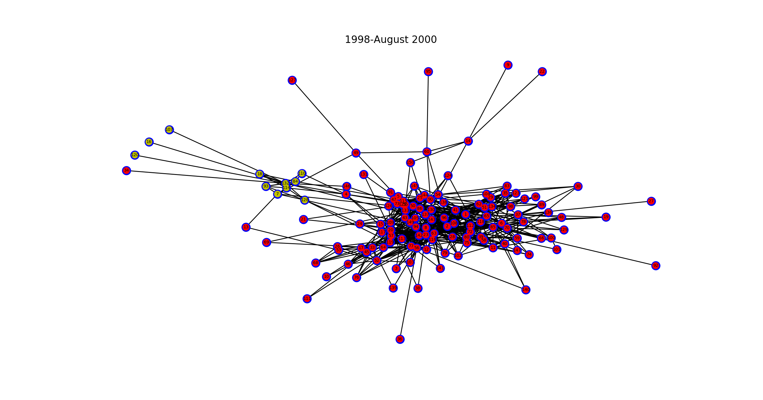
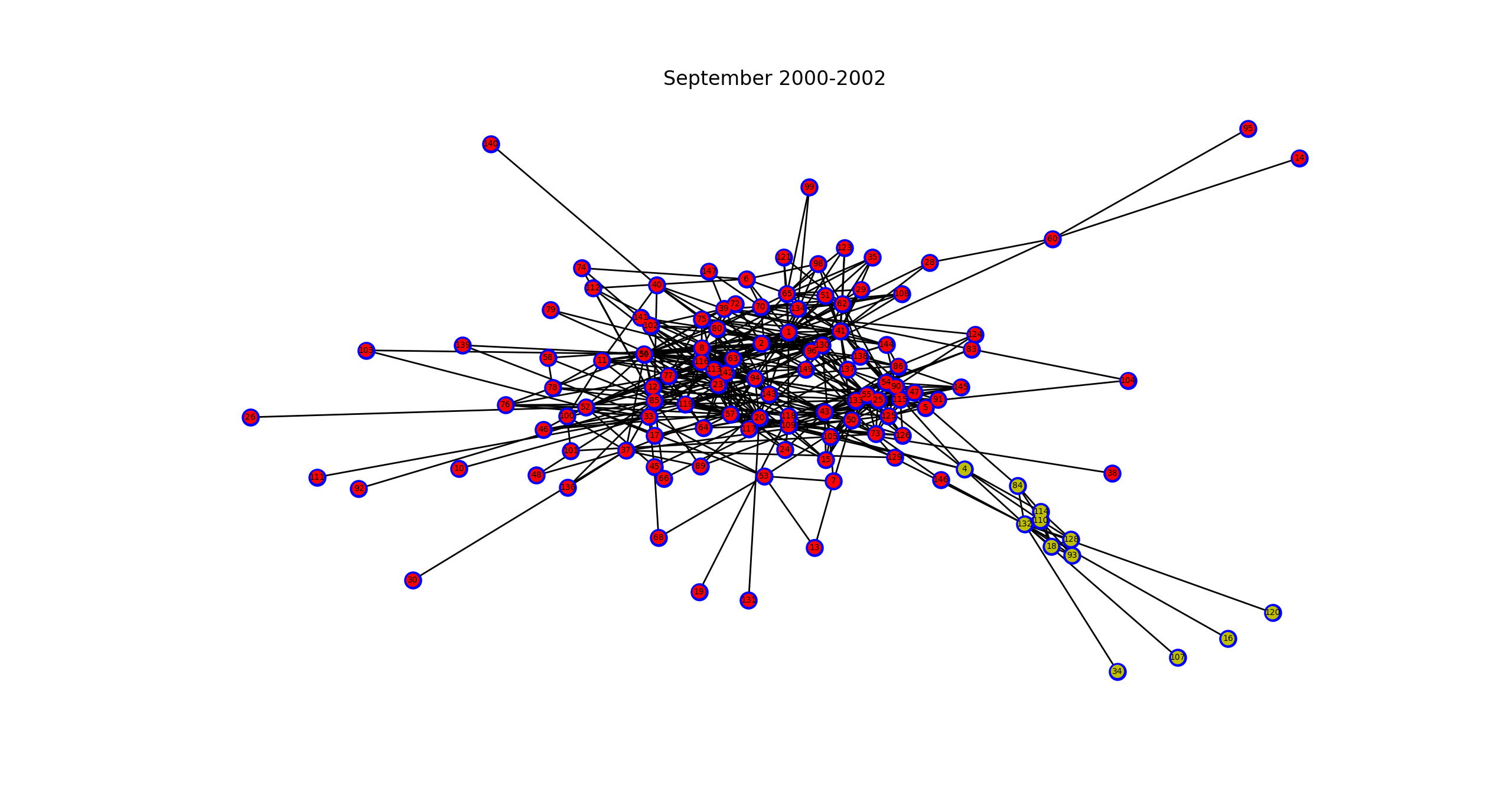
Figure 1: Estimated Enron email networks before and after August 2000.

7.2 Comparing email networks before and after December 2001

We then compared the email networks before and after December 2001, where 7713 emails and 3826 emails were observed, respectively. Our test statistic (4.4) rejected the null, indicating that the community memberships were different before and after December 2001. The date was chosen since CEO Jeffrey Skilling resigned on Aug. 14th, 2001 and the number of emails sent by week revealed peaks in email activity around Nov. 9th 2001 and end of Dec 2001.

Figure 2 shows the two estimated email networks with coordinates generated by Fruchterman-Reingold force-directed algorithm. We observed that weight matrix ${\mathbb{W}}_{n}^{(1)}$ from 1998 to 2000 resulted in a smaller cluster with nodes $[4,16,18,34,93,107,110,114,128,132]$. In contrast, weight matrix ${\mathbb{W}}_{n}^{(2)}$ in 2001 results in two clusters: the smaller cluster has nodes
$[3,32,93,110,114,121,122,132,138]$. Nodes [93, 110, 132] were shared between the two smaller communities, which includes 2 Vice Presidents [93, 132] and a Trader [110] (see Table 7.1).

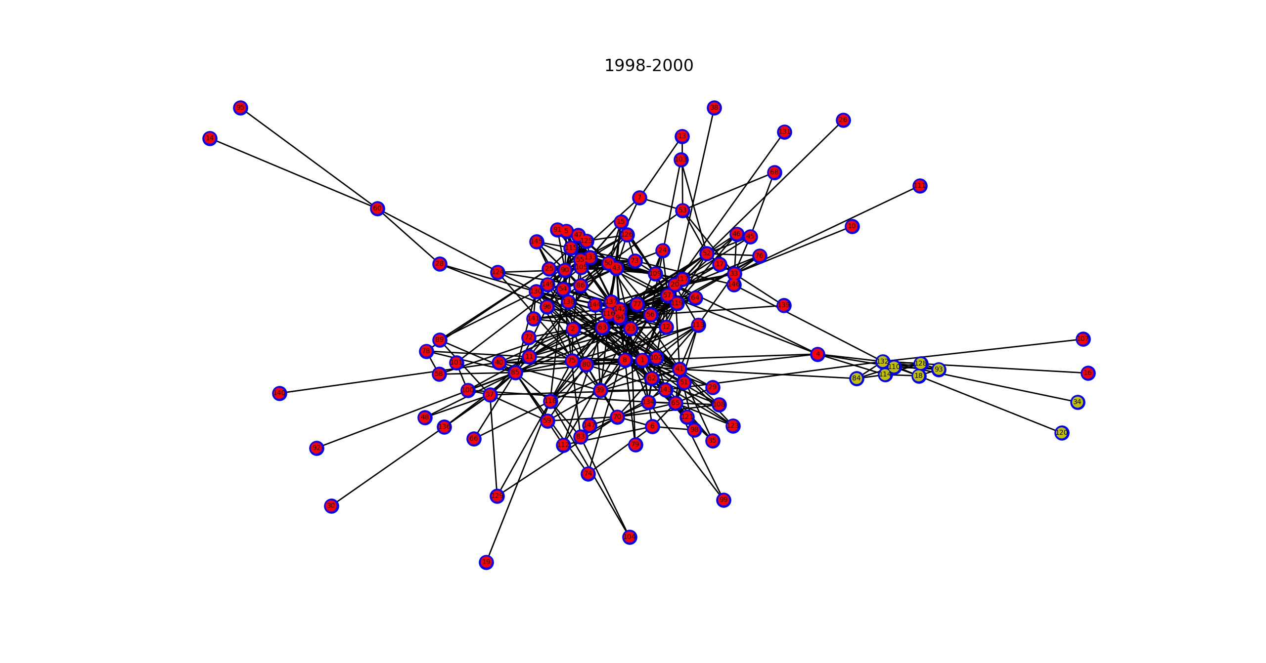
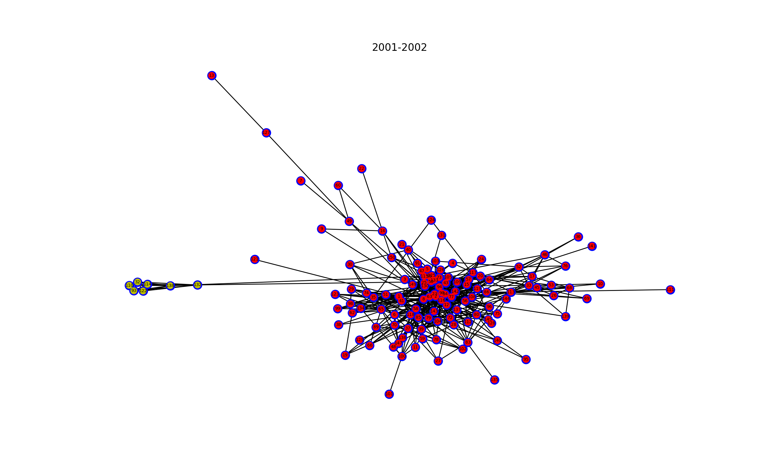
Figure 2: Estimated Enron email networks before and after December 2001.

8 Discussions

We have developed a statistical test for equivalent community memberships based on stochastic block models and derived its asymptotic null distribution under the dense graph assumption (Assumption 3). This assumption is needed to obtain the dominant representation for the subspace distance. In order to detect the community structures, we also require that the intra- and inter-cluster probability distributions are not too close. While this assumption is reasonable, it would be interesting to further investigate the case when the intra- and inter- distributions ${\cal P}_{n},{\cal Q}_{n}$ are close to each other as $n\to\infty$. Like Tang et al. (2017b), we also assume that the distributions that generate the two weighted networks only differ by a scalar. For the case when we have two communities for each network, our test statistic has correct type I errors and large power in detecting the difference in community memberships. When ${K}>2$, estimation of the community memberships becomes more difficult, which can lead to slower convergence rates (see Table H.1 in Supplemental Materials), although type I errors are still approximately under control.

The test procedure we developed is based on community recovery from the observed weighted adjacency matrices (Bickel and Sarkar, 2016; Jog and Loh, 2015a; Lei et al., 2015, 2016; Xu, Jog and Loh, 2017). Alternatively, one can also apply spectral clustering method based on singular components of normalized Laplacian (Rohe et al., 2011; Sarkar et al., 2015) of the corresponding network graphs. It is also interesting to consider kernelized spectral clustering of samples from a finite mixture of nonparametric distributions (Schiebinger et al., 2015). As a future research topic, it is interesting to investigate whether the asymptotic results still hold when these alternative clustering methods are applied.

Assumptions 2 and 4 and including ${\Lambda}_{{\mathbb{W}}_{n}^{(2)}}$ in the proposed test statistic (4.4) are all imposed to simplify the mean and variance of test statistic (4.4). If we impose the “equal-size” assumption (see section 5.2), where $\frac{n}{{K}}$ is assumed to be an integer and $\beta=1$ in Assumption 1 (Banerjee et al., 2018; Banerjee and Ma, 2017), we may relax Assumptions 2 and 4 and eliminate the adjustment of multiplying ${\Lambda}_{{\mathbb{W}}_{n}^{(2)}}$ in test statistic (4.4). This assumption may also possibly relax the requirement that the two distributions that generate the weighted networks differ only by a scalar.

Appendix A Notations

We clarify some notations to facilitate readers’ understanding of statements and proofs of the theorems.

Besides Frobenius norm, we also use 2-norm in the proofs, which is a special case of induced norms (G.1):

$$\|{\mathbb{M}}\|_{2}\triangleq\sup_{\|{\mathbf{x}}\|_{2}=1,{\mathbf{x}}\in{\rm I\!R}^{d}}\|{\mathbb{M}}{\mathbf{x}}\|_{2}=\sqrt{\rho\left({\mathbb{M}}^{T}{\mathbb{M}}\right)},{\mathbb{M}}\in{\rm I\!R}^{m\times d}.$$ (A.1)

where $\rho:{\rm I\!R}^{m\times m}\to{\rm I\!R}^{1}$ refers to spectral radius of a square matrix:

$$\rho({\mathbb{M}})\triangleq\max\left\{\left|\lambda_{1}\left({\mathbb{M}}\right)\right|,\ldots,\left|\lambda_{m}\left({\mathbb{M}}\right)\right|\right\}=\lim_{k\to\infty}\|{\mathbb{M}}^{k}\|^{\frac{1}{k}},$$ (A.2)

for any consistent matrix norm $\|\cdot\|$. In general, $\rho({\mathbb{M}})\leq\|{\mathbb{M}}\|_{2}$, for symmetric matrix ${\mathbb{M}}={\mathbb{M}}^{T}\in{\rm I\!R}^{m\times m}$, $\|{\mathbb{M}}\|_{2}=\rho({\mathbb{M}})$.

When writing $O_{P}(\cdot),O(\cdot),o_{P}(\cdot),o(\cdot)$ with respect to a $m\times d$ matrix, we generally refers (if no any other special instructions) to the order with respect to its Frobenius norm. $f(n)=\Theta(n^{-\alpha})$ or $f(n)\asymp n^{-\alpha}$ mean that there exists constant $C>1$ such that $\frac{n^{-\alpha}}{C}\leq f(n)\leq Cn^{-\alpha}$. The equivalent symbols used in this work are summarized in Table A.1.

Table A.1: Equivalent symbols used in different scenarios.

$O_{P}(\cdot)$	$O(\cdot)$	$o_{P}(\cdot)$	$o(\cdot)$	$\Theta_{P}(n^{-\alpha})$	$\Theta(n^{-\alpha})$
$\preceq_{P}$	$\preceq$	–	–	$\asymp_{P}$	$\asymp$

Appendix B Proof sketch for the asymptotic expansions in Theorem 2 and Theorem 4

We present in this section a sketch of the main ideas in the proofs of Theorem 2 and Theorem 4.

Compared to the proof of Lemma 1 that uses the same technique as in Tang et al. (2017b, 2018), it suffices to provide upper bounds for the difference of the squares of Frobenous norms.

For the case of one-network in Theorem 2, we obtain the following bound

$$\frac{\left\|\left(\mathbb{V}_{{\mathbb{W}}_{n}}\mathbb{T}_{n}-\mathbb{V}_{\mathbb{E}_{n}}\right){\Lambda}_{\mathbb{E}_{n}}\right\|_{F}^{2}}{{K}n}-\frac{\left\|\left({\mathbb{W}}_{n}-\mathbb{E}_{n}\right)\mathbb{V}_{\mathbb{E}_{n}}\right\|_{F}^{2}}{{K}n}=O_{P}\left(\frac{{K}^{2}[\log(n)]^{2}}{n}\right),$$ (B.1)

where $\mathbb{T}_{n}={{\cal P}\mathcal{T}}\left(\mathbb{V}_{{\mathbb{W}}_{n}},\mathbb{V}_{\mathbb{E}_{n}}\right),\mathbb{T}_{n}=\mathbb{V}_{{\mathbb{W}}_{n}}^{T}\mathbb{V}_{\mathbb{E}_{n}}$ or $\left(\mathbb{V}_{\mathbb{E}_{n}}^{T}\mathbb{V}_{{\mathbb{W}}_{n}}\right)^{-1}$. We consider three different $\mathbb{T}_{n}$s for two reasons. First, the proof of (B.1) can be simplified by focusing on $\mathbb{T}_{n}=\left(\mathbb{V}_{\mathbb{E}_{n}}^{T}\mathbb{V}_{{\mathbb{W}}_{n}}\right)^{-1}$. Second, result for (B.1) with $\mathbb{T}_{n}=\mathbb{V}_{{\mathbb{W}}_{n}}^{T}\mathbb{V}_{\mathbb{E}_{n}}$ has a direct Corollary C.13 that can simplify the proof of Theorem 4 since it simplifies the proof for (B).

For the two-sample case in Theorem 4, under the null hypothesis (4.3), we have the bound for the difference of the squares of Frobenous norms

$$\frac{1}{{K}n}\left\|\left(\mathbb{V}_{{\mathbb{W}}_{n}^{(1)}}\mathbb{T}_{n}-\mathbb{V}_{{\mathbb{W}}_{n}^{(2)}}\right){\Lambda}_{{\mathbb{W}}_{n}^{(2)}}\right\|_{F}^{2}-\frac{1}{{K}n}\left\|\left(\gamma{\mathbb{W}}_{n}^{(1)}-{\mathbb{W}}_{n}^{(2)}\right)\mathbb{V}_{\mathbb{E}_{n}^{(2)}}\right\|_{F}^{2}$$

$$= O_{P}\left(\frac{{K}^{2}[\log(n)]^{2}}{n}\right),$$

where

$$\mathbb{T}_{n}={{\cal P}\mathcal{T}}\left(\mathbb{V}_{{\mathbb{W}}_{n}^{(1)}},\mathbb{V}_{{\mathbb{W}}_{n}^{(2)}}\right),\mathbb{V}_{{\mathbb{W}}_{n}^{(1)}}^{T}\mathbb{V}_{{\mathbb{W}}_{n}^{(2)}},\mbox{ or }\left(\mathbb{V}_{{\mathbb{W}}_{n}^{(2)}}^{T}\mathbb{V}_{{\mathbb{W}}_{n}^{(1)}}\right)^{-1}.$$

To conclude, these two bounds are used to prove asymptotic expansions in Theorem 2 and Theorem 4, respectively.

B.1 Proof sketch for the asymptotic expansion in Theorem 2

To prove (B.1), we first focus on proving the result for $\mathbb{T}_{n}=\left(\mathbb{V}_{{\mathbb{W}}_{n}}^{T}\mathbb{V}_{\mathbb{E}_{n}}\right)^{-1}$ in Section C.2.1. Its proof is briefly sketched as the following:

$$\frac{1}{{K}n}\left\|\left(\mathbb{V}_{{\mathbb{W}}_{n}}\left(\mathbb{V}_{\mathbb{E}_{n}}^{T}\mathbb{V}_{{\mathbb{W}}_{n}}\right)^{-1}-\mathbb{V}_{\mathbb{E}_{n}}\right){\Lambda}_{\mathbb{E}_{n}}\right\|_{F}^{2}$$

$$\xlongequal{\text{\eqref{eq: part using the fact that E = VEVET E}}} \frac{1}{{K}n}\left\|\left(\mathbb{I}_{n}-\mathbb{V}_{\mathbb{E}_{n}}\mathbb{V}_{\mathbb{E}_{n}}^{T}\right)\left({\mathbb{W}}_{n}-\mathbb{E}_{n}\right)\mathbb{V}_{{\mathbb{W}}_{n}}\left(\mathbb{V}_{\mathbb{E}_{n}}^{T}\mathbb{V}_{{\mathbb{W}}_{n}}\right)^{-1}\right\|_{F}^{2}+O_{P}\left(\frac{{K}^{2}\log(n)}{n^{2}b_{{\cal P}}^{\frac{3}{2}}}\right)$$

$$= \frac{1}{{K}n}\left\|\left({\mathbb{W}}_{n}-\mathbb{E}_{n}\right)\mathbb{V}_{{\mathbb{W}}_{n}}\left(\mathbb{V}_{\mathbb{E}_{n}}^{T}\mathbb{V}_{{\mathbb{W}}_{n}}\right)^{-1}\right\|_{F}^{2}$$

$$-\frac{1}{{K}n}\left\|\mathbb{V}_{\mathbb{E}}^{T}\left({\mathbb{W}}_{n}-\mathbb{E}_{n}\right)\mathbb{V}_{{\mathbb{W}}_{n}}\left(\mathbb{V}_{\mathbb{E}_{n}}^{T}\mathbb{V}_{{\mathbb{W}}_{n}}\right)^{-1}\right\|_{F}^{2}+O_{P}\left(\frac{{K}^{2}\log(n)}{n^{2}b_{{\cal P}}^{\frac{3}{2}}}\right)$$

$$\xlongequal{\text{\eqref{eq:term Wigner order}}} \frac{1}{{K}n}\left\|\left({\mathbb{W}}_{n}-\mathbb{E}_{n}\right)\mathbb{V}_{{\mathbb{W}}_{n}}\left(\mathbb{V}_{\mathbb{E}_{n}}^{T}\mathbb{V}_{{\mathbb{W}}_{n}}\right)^{-1}\right\|_{F}^{2}+O_{P}\left(\frac{{K}[\log(n)]^{2}}{n}\right)$$

$$\xlongequal{\text{\eqref{eq:my B8 AJ}}} \frac{1}{{K}n}\left\|\left({\mathbb{W}}_{n}-\mathbb{E}_{n}\right)\mathbb{V}_{\mathbb{E}_{n}}\right\|_{F}^{2}+O_{P}\left(\frac{{K}[\log(n)]^{2}}{n}\right).$$

For $\mathbb{T}_{n}={{\cal P}\mathcal{T}}\left(\mathbb{V}_{{\mathbb{W}}_{n}},\mathbb{V}_{\mathbb{E}_{n}}\right)$, we need to consider the difference of two squares of Frobenius norm,

$$\frac{1}{{K}n}\left\|\left(\mathbb{V}_{{\mathbb{W}}_{n}}\mathbb{V}_{{\mathbb{W}}_{n}}^{T}\mathbb{V}_{\mathbb{E}_{n}}-\mathbb{V}_{\mathbb{E}_{n}}\right){\Lambda}_{\mathbb{E}_{n}}\right\|_{F}^{2}-\frac{1}{{K}n}\left\|\left(\mathbb{V}_{{\mathbb{W}}_{n}}\tilde{\mathbb{T}}_{n}-\mathbb{V}_{\mathbb{E}_{n}}\right){\Lambda}_{\mathbb{E}_{n}}\right\|_{F}^{2},$$

that is, left-hand side of (B.1) with $\mathbb{T}_{n}=\mathbb{V}_{{\mathbb{W}}_{n}}^{T}\mathbb{V}_{\mathbb{E}_{n}}$ and $\mathbb{T}_{n}=\tilde{\mathbb{T}}_{n}$ where (C.11) holds:

$$\left\|\mathbb{V}_{{\mathbb{W}}_{n}}^{T}\mathbb{V}_{\mathbb{E}_{n}}-\tilde{\mathbb{T}}_{n}\right\|_{F}=O_{P}\left(\frac{{K}^{2}}{nb_{{\cal P}}}\log(n)\right).$$

The difference can be upper-bounded as (C.12)

$$\frac{1}{{K}n}\left\|\left(\mathbb{V}_{{\mathbb{W}}_{n}}\mathbb{V}_{{\mathbb{W}}_{n}}^{T}\mathbb{V}_{\mathbb{E}_{n}}-\mathbb{V}_{\mathbb{E}_{n}}\right){\Lambda}_{\mathbb{E}_{n}}\right\|_{F}^{2}-\frac{1}{{K}n}\left\|\left(\mathbb{V}_{{\mathbb{W}}_{n}}\tilde{\mathbb{T}}_{n}-\mathbb{V}_{\mathbb{E}_{n}}\right){\Lambda}_{\mathbb{E}_{n}}\right\|_{F}^{2}$$

$$\xlongequal{\text{\eqref{eq:requirement for tilde Tn}}} \frac{2}{{K}n}\left\langle\mathbb{V}_{{\mathbb{W}}_{n}}\left(\mathbb{V}_{{\mathbb{W}}_{n}}^{T}\mathbb{V}_{\mathbb{E}_{n}}-\tilde{\mathbb{T}}_{n}\right){\Lambda}_{\mathbb{E}_{n}},\left(\mathbb{V}_{{\mathbb{W}}_{n}}\mathbb{V}_{{\mathbb{W}}_{n}}^{T}\mathbb{V}_{\mathbb{E}_{n}}-\mathbb{V}_{\mathbb{E}_{n}}\right){\Lambda}_{\mathbb{E}_{n}}\right\rangle$$

$$+O_{P}\left(\frac{{K}[\log(n)]^{2}}{n}\right)$$

$$\xlongequal{\mathbb{V}_{{\mathbb{W}}_{n}}^{T}\mathbb{V}_{{\mathbb{W}}_{n}}\mathbb{V}_{{\mathbb{W}}_{n}}^{T}=\mathbb{V}_{{\mathbb{W}}_{n}}^{T}}0+O_{P}\left(\frac{1}{n}\right)=O_{P}\left(\frac{{K}[\log(n)]^{2}}{n}\right).$$

With these results and the proof of (B.1) for $\left(\mathbb{V}_{{\mathbb{W}}_{n}}^{T}\mathbb{V}_{\mathbb{E}_{n}}\right)^{-1}$, we take $\tilde{\mathbb{T}}_{n}=\left(\mathbb{V}_{{\mathbb{W}}_{n}}^{T}\mathbb{V}_{\mathbb{E}_{n}}\right)^{-1}$ in (C.12) and we prove that (B.1) holds for $\mathbb{T}_{n}=\mathbb{V}_{\mathbb{E}_{n}}^{T}\mathbb{V}_{{\mathbb{W}}_{n}}$. With this result, we take $\mathbb{T}_{n}={{\cal P}\mathcal{T}}\left(\mathbb{V}_{{\mathbb{W}}_{n}},\mathbb{V}_{\mathbb{E}_{n}}\right)$ in (C.12) and we prove that (B.1) holds for $\mathbb{T}_{n}={{\cal P}\mathcal{T}}\left(\mathbb{V}_{{\mathbb{W}}_{n}},\mathbb{V}_{\mathbb{E}_{n}}\right)$.

B.2 Proof sketch for asymptotic expansion in Theorem 4

For the two-sample results stated in Theorem 4, it is worth mentioning that an essential difficulty that makes the two-sample problem more difficult than the problem with one network is that ${\mathbb{W}}_{n}^{(v)}\neq\mathbb{V}_{{\mathbb{W}}_{n}^{(v)}}\mathbb{V}_{{\mathbb{W}}_{n}^{(v)}}^{T}{\mathbb{W}}_{n}^{(v)}$. However, equality $\mathbb{E}_{n}=\mathbb{V}_{\mathbb{E}_{n}}\mathbb{V}_{\mathbb{E}_{n}}^{T}\mathbb{E}_{n}$ is used in the above proof sketch for (B.1) in step (C.2.1). In contrast, for the two-sample problem, we do not have such an equality.

To prove (B), we first consider $\mathbb{T}_{n}=\mathbb{V}_{{\mathbb{W}}_{n}^{(1)}}^{T}\mathbb{V}_{{\mathbb{W}}_{n}^{(2)}}$. With details given in Section C.3, steps at the beginning are sketched as the following:

$$\frac{\left\|\left(\mathbb{V}_{{\mathbb{W}}_{n}^{(1)}}\mathbb{V}_{{\mathbb{W}}_{n}^{(1)}}^{T}\mathbb{V}_{{\mathbb{W}}_{n}^{(2)}}-\mathbb{V}_{{\mathbb{W}}_{n}^{(2)}}\right){\Lambda}_{{\mathbb{W}}_{n}^{(2)}}\right\|_{F}^{2}}{{K}n}-\frac{\left\|\left(\gamma{\mathbb{W}}^{(1)}-{\mathbb{W}}_{n}^{(2)}\right)\mathbb{V}_{{\mathbb{W}}_{n}^{(2)}}\right\|_{F}^{2}}{{K}n}$$

$$= \frac{\left\|\left(\mathbb{V}_{{\mathbb{W}}_{n}^{(1)}}\mathbb{V}_{{\mathbb{W}}_{n}^{(1)}}^{T}-\mathbb{I}_{n}\right){\mathbb{W}}_{n}^{(2)}\mathbb{V}_{{\mathbb{W}}_{n}^{(2)}}\right\|_{F}^{2}}{{K}n}-\frac{\left\|\left(\gamma{\mathbb{W}}_{n}^{(1)}-{\mathbb{W}}_{n}^{(2)}\right)\mathbb{V}_{{\mathbb{W}}_{n}^{(2)}}\right\|_{F}^{2}}{{K}n}$$

$$= \frac{1}{{K}n}\left\langle\left(\mathbb{V}_{{\mathbb{W}}_{n}^{(1)}}\mathbb{V}_{{\mathbb{W}}_{n}^{(1)}}^{T}-\mathbb{I}_{n}\right){\mathbb{W}}^{(2)}\mathbb{V}_{{\mathbb{W}}_{n}^{(2)}},\right.$$

$$\left.\left(\mathbb{V}_{{\mathbb{W}}_{n}^{(1)}}\mathbb{V}_{{\mathbb{W}}_{n}^{(1)}}^{T}-\mathbb{I}_{n}\right){\mathbb{W}}_{n}^{(2)}\mathbb{V}_{{\mathbb{W}}_{n}^{(2)}}-\left(\gamma{\mathbb{W}}_{n}^{(1)}-{\mathbb{W}}_{n}^{(2)}\right)\mathbb{V}_{{\mathbb{W}}_{n}^{(2)}}\right\rangle$$

$$+O_{P}\left(\frac{{K}[\log(n)]^{2}}{n}\right)$$

$$= \frac{1}{{K}n}\left\langle\left(\mathbb{V}_{{\mathbb{W}}_{n}^{(1)}}\mathbb{V}_{{\mathbb{W}}_{n}^{(1)}}^{T}-\mathbb{I}_{n}\right){\mathbb{W}}_{n}^{(2)}\mathbb{V}_{{\mathbb{W}}_{n}^{(2)}},\left(\mathbb{V}_{{\mathbb{W}}_{n}^{(1)}}\mathbb{V}_{{\mathbb{W}}_{n}^{(1)}}^{T}{\mathbb{W}}_{n}^{(2)}-\gamma{\mathbb{W}}_{n}^{(1)}\right)\mathbb{V}_{{\mathbb{W}}_{n}^{(2)}}\right\rangle$$

$$+O_{P}\left(\frac{{K}[\log(n)]^{2}}{n}\right)$$

$$= -\frac{\gamma}{{K}n}{\rm tr}\left[\mathbb{V}_{{\mathbb{W}}_{n}^{(2)}}^{T}{\mathbb{W}}_{n}^{(1)}\left(\mathbb{V}_{{\mathbb{W}}_{n}^{(1)}}\mathbb{V}_{{\mathbb{W}}_{n}^{(1)}}^{T}-\mathbb{I}_{n}\right){\mathbb{W}}_{n}^{(2)}\mathbb{V}_{{\mathbb{W}}_{n}^{(2)}}\right]+O_{P}\left(\frac{{K}[\log(n)]^{2}}{n}\right)$$

$$= -\frac{\gamma}{{K}n}{\rm tr}\left[\mathbb{V}_{{\mathbb{W}}_{n}^{(2)}}^{T}\mathbb{V}_{{\mathbb{W}}_{n}^{(1)}}^{\perp}{\Lambda}_{{\mathbb{W}}_{n}^{(1)}}^{\perp}\left[\mathbb{V}_{{\mathbb{W}}_{n}^{(1)}}^{\perp}\right]^{T}\mathbb{V}_{{\mathbb{W}}_{n}^{(2)}}{\Lambda}_{{\mathbb{W}}_{n}^{(2)}}\right]+O_{P}\left(\frac{{K}[\log(n)]^{2}}{n}\right).$$

To continue proving (B) with $\mathbb{T}_{n}=\mathbb{V}_{{\mathbb{W}}_{n}^{(1)}}^{T}\mathbb{V}_{{\mathbb{W}}_{n}^{(2)}}$, we need to show that

$$\frac{\gamma}{{K}n}{\rm tr}\left[\mathbb{V}_{{\mathbb{W}}_{n}^{(2)}}^{T}\mathbb{V}_{{\mathbb{W}}_{n}^{(1)}}^{\perp}{\Lambda}_{{\mathbb{W}}_{n}^{(1)}}^{\perp}\left[\mathbb{V}_{{\mathbb{W}}_{n}^{(1)}}^{\perp}\right]^{T}\mathbb{V}_{{\mathbb{W}}_{n}^{(2)}}{\Lambda}_{{\mathbb{W}}_{n}^{(2)}}\right]=O_{P}\left(\frac{{K}[\log(n)]^{2}}{n}\right),$$

and the same result holds when

$$\frac{\left\|\left(\gamma{\mathbb{W}}_{n}^{(1)}-{\mathbb{W}}_{n}^{(2)}\right)\mathbb{V}_{{\mathbb{W}}_{n}^{(2)}}\right\|_{F}^{2}}{{K}n}$$

is replaced with

$$-\frac{\left\|\left(\gamma{\mathbb{W}}_{n}^{(1)}-{\mathbb{W}}_{n}^{(2)}\right)\mathbb{V}_{\mathbb{E}^{(2)}}\right\|_{F}^{2}}{{K}n}.$$

The proofs of these two steps are supported by Corollary C.13 and Corollary 12 in Section C.3.1. These two corollaries are essentially derived from the proof for the problem of one network in Section C.2.

We outline the proof of Corollary C.13 to demonstrate how we overcome the essential difficulty mentioned above. This Corollary is derived from the result for $\mathbb{T}_{n}=\mathbb{V}_{\mathbb{E}_{n}}^{T}\mathbb{V}_{{\mathbb{W}}_{n}}$ in (B.1) rather than a direct corollary of the discussion in Section C.2.1 of $\mathbb{T}=\left(\mathbb{V}_{{\mathbb{W}}_{n}}^{T}\mathbb{V}_{\mathbb{E}_{n}}\right)^{-1}$ in (B.1). Corollary C.13 states that (C.13) holds, that is

$${\rm tr}\left[\mathbb{V}_{\mathbb{E}_{n}}^{T}\mathbb{V}_{{\mathbb{W}}_{n}}^{\perp}{\Lambda}_{{\mathbb{W}}_{n}}^{\perp}\left[\mathbb{V}_{{\mathbb{W}}_{n}}^{\perp}\right]^{T}\mathbb{V}_{\mathbb{E}_{n}}\right]=O_{P}\left({K}^{2}[\log(n)]^{2}\right),$$

which implies

$$O_{P}\left({K}\log(n)\right)$$

$$= \sqrt{{\rm tr}\left[\mathbb{V}_{\mathbb{E}_{n}^{(1)}}^{T}\mathbb{V}_{{\mathbb{W}}_{n}^{(1)}}^{\perp}{\Lambda}_{{\mathbb{W}}_{n}^{(1)}}^{\perp}\left[\mathbb{V}_{{\mathbb{W}}_{n}^{(1)}}^{\perp}\right]^{T}\mathbb{V}_{\mathbb{E}_{n}^{(1)}}\right]}$$

$$= \left\|\left[{\Lambda}_{{\mathbb{W}}_{n}^{(1)}}^{\perp}\right]^{\frac{1}{2}}\left[\mathbb{V}_{{\mathbb{W}}^{(1)}}^{\perp}\right]^{T}\mathbb{V}_{\mathbb{E}_{n}^{(1)}}\right\|_{F}=\left\|\left[{\Lambda}_{{\mathbb{W}}_{n}^{(1)}}^{\perp}\right]^{\frac{1}{2}}\left[\mathbb{V}_{{\mathbb{W}}_{n}^{(1)}}^{\perp}\right]^{T}\mathbb{V}_{\mathbb{E}_{n}^{(2)}}\right\|_{F}$$

$$= \left\|\left[{\Lambda}_{{\mathbb{W}}_{n}^{(1)}}^{\perp}\right]^{\frac{1}{2}}\left[\mathbb{V}_{{\mathbb{W}}_{n}^{(1)}}^{\perp}\right]^{T}\cdot\right.\left.\left[\mathbb{V}_{\mathbb{E}_{n}^{(2)}}-\mathbb{V}_{{\mathbb{W}}_{n}^{(2)}}{{\cal P}\mathcal{T}}\left(\mathbb{V}_{{\mathbb{W}}_{n}^{(2)}},\mathbb{V}_{\mathbb{E}_{n}^{(2)}}\right)+\mathbb{V}_{{\mathbb{W}}_{n}^{(2)}}{{\cal P}\mathcal{T}}\left(\mathbb{V}_{{\mathbb{W}}_{n}^{(2)}},\mathbb{V}_{\mathbb{E}_{n}^{(2)}}\right)\right]\right\|_{F}$$

$$= \left\|\left[{\Lambda}_{{\mathbb{W}}_{n}^{(1)}}^{\perp}\right]^{\frac{1}{2}}\left[\mathbb{V}_{{\mathbb{W}}_{n}^{(1)}}^{\perp}\right]^{T}\mathbb{V}_{{\mathbb{W}}_{n}^{(2)}}{{\cal P}\mathcal{T}}\left(\mathbb{V}_{{\mathbb{W}}_{n}^{(2)}},\mathbb{V}_{\mathbb{E}_{n}^{(2)}}\right)\right\|_{F}+O_{P}\left(\sqrt{\frac{{K}}{nb_{{\cal P}}}}\cdot\sqrt{\frac{nb_{{\cal P}}}{{K}}}\right)$$

$$= \left\|\left[{\Lambda}_{{\mathbb{W}}_{n}^{(1)}}^{\perp}\right]^{\frac{1}{2}}\left[\mathbb{V}_{{\mathbb{W}}_{n}^{(1)}}^{\perp}\right]^{T}\mathbb{V}_{{\mathbb{W}}_{n}^{(2)}}\right\|_{F}+O_{P}\left(\sqrt{{K}b_{{\cal P}}}\right),$$

where $\left[{\Lambda}_{{\mathbb{W}}_{n}^{(1)}}^{\perp}\right]^{\frac{1}{2}}\triangleq{\rm diag}\left\{\left|\sigma_{{K}+1}\left({\mathbb{W}}_{n}^{(1)}\right)\right|^{\frac{1}{2}},\ldots,\left|\sigma_{n}\left({\mathbb{W}}_{n}^{(1)}\right)\right|^{\frac{1}{2}}\right\}$. This equivalently implies that

$$-\frac{\gamma}{{K}n}{\rm tr}\left[\mathbb{V}_{{\mathbb{W}}_{n}^{(2)}}^{T}\mathbb{V}_{{\mathbb{W}}_{n}^{(1)}}^{\perp}{\Lambda}_{{\mathbb{W}}_{n}^{(1)}}^{\perp}\left[\mathbb{V}_{{\mathbb{W}}_{n}^{(1)}}^{\perp}\right]^{T}\mathbb{V}_{{\mathbb{W}}_{n}^{(2)}}{\Lambda}_{{\mathbb{W}}_{n}^{(2)}}\right]$$

$$= -\frac{\gamma}{{K}n}\left\|\left[{\Lambda}_{{\mathbb{W}}_{n}^{(1)}}^{\perp}\right]^{\frac{1}{2}}\left[\mathbb{V}_{{\mathbb{W}}_{n}^{(1)}}^{\perp}\right]^{T}\mathbb{V}_{{\mathbb{W}}_{n}^{(2)}}\right\|_{F}^{2}=O_{P}\left(\frac{{K}[\log(n)]^{2}}{n}\right).$$

With this result, we arrives at Lemma 14:

$$\frac{\left\|\left(\mathbb{V}_{{\mathbb{W}}_{n}^{(1)}}\mathbb{T}-\mathbb{V}_{{\mathbb{W}}_{n}^{(2)}}\right){\Lambda}_{{\mathbb{W}}_{n}^{(2)}}\right\|_{F}^{2}}{{K}n}=\frac{\left\|\left(\gamma{\mathbb{W}}_{n}^{(1)}-{\mathbb{W}}_{n}^{(2)}\right)\mathbb{V}_{{\mathbb{W}}_{n}^{(2)}}\right\|_{F}^{2}}{{K}n}+O_{P}\left(\frac{{K}[\log(n)]^{2}}{n}\right).$$

Finally, together with further argument using Corollary 12, we obtains (B).

Supplementary Material

Supplement to ”Two-sample test of community memberships of weighted stochastic block models” (.pdf file). The supplement includes: (i) proofs of all theoretical results in the main paper, (ii) additional technical tools and supporting lemmas, and (iii) additional numerical results when the number of communities is greater than 2.

Appendix C Proofs of asymptotic expansions of the singular subspace distances

In this Section, we present proof of Lemma 1, Theorem 2 and Theorem 4 for the asymptotic expansions of the singular subspace distances. In the following proofs, we may ignore the subscript $n$ when no confusion exists. These asymptotic expansions are needed to derive the asymptotic distribution of the proposed test statistic.

C.1 Proof of Lemma 1

The techniques to prove Lemma 1 are similar to (2.5) of Theorem 3.1 in Tang et al. (2018). We briefly outline the proof here.

First notice that (D.1), which we derive later on, says

$$\frac{\left\|\left({\mathbb{W}}_{n}-\mathbb{E}_{n}\right)\mathbb{V}_{\mathbb{E}_{n}}\right\|_{F}^{2}}{{K}nb_{{\cal P}}}=\frac{({K}-1)n\sigma_{Q}^{2}+n\sigma_{P}^{2}+o\left(n\sigma_{{\cal P}}^{2}\right)}{{K}nb_{{\cal P}}}=O_{P}(1),$$

which implies

$$\frac{\left\|\left({\mathbb{W}}_{n}-\mathbb{E}_{n}\right)\mathbb{V}_{\mathbb{E}_{n}}\right\|_{F}}{\sqrt{{K}nb_{{\cal P}}}}=O_{P}(1).$$ (C.1)

Second, for the asymptotic expansion, instead of using spectral embeddings as in Tang et al. (2017b, 2018), we have singular vector matrices. For convenience, instead of writing transformation $\mathbb{T}$ on the left $n\times{K}$ matrix as it appeared in (1), we write it on the right $n\times{K}$ matrix – this follows the style that although (2.5) in Theorem 2.1 and (3.1) in Theorem 3.1 of Tang et al. (2018) has orthogonal matrix multiplying on the left one, Section (B.19-22) in B.2 of Tang et al. (2018) has it mutiplying on the right one.

Before our derivation, we present Corollary 9, which is a consequence of Davis-Kahan $\sin\Theta$ theorem. Although some classical forms are in Stewart and Sun (1990); Davis and Kahan (1970), we present Davis-Kahan $\sin\Theta$ theorem in the context of our setting, which is analogous to Hsu (Accessed: 2016):

Lemma 8 (Davis-Kahan $\sin\Theta$).

Denote singular value decomposition of ${\mathbb{W}}_{n}$ as ${\mathbb{W}}_{n}=\mathbb{V}_{{\mathbb{W}}_{n}}{\Lambda}_{{\mathbb{W}}_{n}}\mathbb{V}_{{\mathbb{W}}_{n}}^{T}+\mathbb{V}_{{\mathbb{W}}_{n}}^{\perp}{\Lambda}_{{\mathbb{W}}_{n}}^{\perp}\left(\mathbb{V}_{{\mathbb{W}}_{n}}^{\perp}\right)^{T}$, and similarly for $\mathbb{E}_{n}$. Suppose $\left\|{\Lambda}_{{\mathbb{W}}_{n}}^{\perp}\right\|_{2}<\left\|{\Lambda}_{\mathbb{E}_{n}}^{-1}\right\|_{2}^{-1}$, where $\left\|{\Lambda}_{\mathbb{E}_{n}}^{-1}\right\|_{2}^{-1}$ is the ${K}$th (absolutely) largest eigenvalue of $\mathbb{E}_{n}$, $\left\|{\Lambda}_{{\mathbb{W}}_{n}}\right\|_{2}$ is the $({K}+1)$th (absolutely) largest eigenvalue of ${\mathbb{W}}_{n}$. Then for any unitarily-invariant norm $\|\cdot\|_{\mathcal{U}}$ (and we focus on $\|\cdot\|_{\mathcal{U}}=\|\cdot\|_{2},\|\cdot\|_{F}$),

$$\left\|\left(\mathbb{V}_{{\mathbb{W}}_{n}}^{\perp}\right)^{T}\mathbb{V}_{\mathbb{E}_{n}}\right\|_{\mathcal{U}}\leq\frac{\left\|\left({\mathbb{W}}_{n}-\mathbb{E}_{n}\right)\mathbb{V}_{\mathbb{E}_{n}}\right\|_{\mathcal{U}}}{\left\|{\Lambda}_{\mathbb{E}_{n}}^{-1}\right\|_{2}^{-1}-\left\|{\Lambda}_{{\mathbb{W}}_{n}}^{\perp}\right\|_{2}},$$

Proof.

For any unitarily invariant norm $\|\cdot\|_{\mathcal{U}}$, we have

$$\left\|\left(\mathbb{V}_{{\mathbb{W}}_{n}}^{\perp}\right)^{T}\left({\mathbb{W}}_{n}-\mathbb{E}_{n}\right)\mathbb{V}_{\mathbb{E}}\right\|_{\mathcal{U}}$$

$$= \left\|\left(\mathbb{V}_{{\mathbb{W}}_{n}}^{\perp}\right)^{T}{\mathbb{W}}_{n}\mathbb{V}_{\mathbb{E}_{n}}-\left(\mathbb{V}_{{\mathbb{W}}_{n}}^{\prime}\right)^{T}\mathbb{E}_{n}\mathbb{V}_{\mathbb{E}_{n}}\right\|_{\mathcal{U}}$$

$$= \left\|{\Lambda}_{{\mathbb{W}}_{n}}^{\perp}\left(\mathbb{V}_{{\mathbb{W}}_{n}}^{\perp}\right)^{T}\mathbb{V}_{\mathbb{E}_{n}}-{\Lambda}_{\mathbb{E}_{n}}\left(\mathbb{V}_{{\mathbb{W}}_{n}}^{\perp}\right)^{T}\mathbb{V}_{\mathbb{E}_{n}}\right\|_{\mathcal{U}}$$

$$= \left\|\left({\Lambda}_{{\mathbb{W}}_{n}}^{\perp}-c\mathbb{I}_{{K}}\right)\left(\mathbb{V}_{{\mathbb{W}}_{n}}^{\prime}\right)^{T}\mathbb{V}_{\mathbb{E}_{n}}-\left({\Lambda}_{\mathbb{E}_{n}}-c\mathbb{I}_{{K}}\right)\left(\mathbb{V}_{{\mathbb{W}}_{n}}^{\perp}\right)^{T}\mathbb{V}_{\mathbb{E}_{n}}-\left({\Lambda}_{{\mathbb{W}}_{n}}^{\perp}\right)\right\|_{\mathcal{U}}$$

$$\geq \left\|\left({\Lambda}_{{\mathbb{W}}_{n}}^{\perp}-c\mathbb{I}_{{K}}\right)\left(\mathbb{V}_{{\mathbb{W}}_{n}}^{\perp}\right)^{T}\mathbb{V}_{\mathbb{E}_{n}}\right)-\rho\left(\left({\Lambda}_{\mathbb{E}_{n}}-c\mathbb{I}_{{K}}\right)\left(\mathbb{V}_{{\mathbb{W}}_{n}}^{\perp}\right)^{T}\mathbb{V}_{\mathbb{E}_{n}}-\left({\Lambda}_{{\mathbb{W}}_{n}}^{\perp}\right)\right\|_{\mathcal{U}},$$

while $c$ can be chosen arbitrarily, we pick $c=\frac{\left\|{\Lambda}_{\mathbb{E}_{n}}\right\|_{2}+\left\|{\Lambda}_{\mathbb{E}_{n}}^{-1}\right\|_{2}^{-1}}{2}$; thus

$$\left\|\left(\mathbb{V}_{{\mathbb{W}}_{n}}^{\perp}\right)^{T}\left({\mathbb{W}}_{n}-\mathbb{E}_{n}\right)\mathbb{V}_{\mathbb{E}}\right\|_{\mathcal{U}}$$

$$\geq \left[\frac{1}{\left\|\left({\Lambda}_{{\mathbb{W}}_{n}}^{\perp}-c\mathbb{I}_{{K}}\right)^{-1}\right\|_{2}}-\left\|{\Lambda}_{\mathbb{E}_{n}}-c\mathbb{I}_{{K}}\right\|_{2}\right]\cdot\left\|\left(\mathbb{V}_{{\mathbb{W}}_{n}}^{\perp}\right)^{T}\mathbb{V}_{\mathbb{E}_{n}}\right\|_{\mathcal{U}}$$

$$= \left[\frac{1}{\left\|\left({\Lambda}_{{\mathbb{W}}_{n}}^{\perp}-c\mathbb{I}_{{K}}\right)^{-1}\right\|_{2}}-\frac{\left\|{\Lambda}_{\mathbb{E}_{n}}\right\|_{2}-\left\|{\Lambda}_{\mathbb{E}_{n}}^{-1}\right\|_{2}^{-1}}{2}\right]\cdot\left\|\left(\mathbb{V}_{{\mathbb{W}}_{n}}^{\perp}\right)^{T}\mathbb{V}_{\mathbb{E}_{n}}\right\|_{\mathcal{U}},$$

where under assumption $\left\|{\Lambda}_{{\mathbb{W}}_{n}}^{\perp}\right\|_{2}<\left\|{\Lambda}_{\mathbb{E}_{n}}^{-1}\right\|_{2}^{-1}$, we have

$$\frac{1}{\left\|\left({\Lambda}_{{\mathbb{W}}_{n}}^{\perp}-c\mathbb{I}_{{K}}\right)^{-1}\right\|_{2}}\geq\frac{\left\|{\Lambda}_{\mathbb{E}_{n}}\right\|_{2}+\left\|{\Lambda}_{\mathbb{E}_{n}}^{-1}\right\|_{2}^{-1}}{2}-\left\|{\Lambda}_{{\mathbb{W}}_{n}}^{\perp}\right\|_{2},$$

thus

$$\left\|\left(\mathbb{V}_{{\mathbb{W}}_{n}}^{\perp}\right)^{T}\left({\mathbb{W}}_{n}-\mathbb{E}_{n}\right)\mathbb{V}_{\mathbb{E}_{n}}\right\|_{\mathcal{U}}\geq\left[\left\|{\Lambda}_{\mathbb{E}_{n}}^{-1}\right\|_{2}^{-1}-\left\|{\Lambda}_{{\mathbb{W}}_{n}}^{\perp}\right\|_{2}\right]\cdot\left\|\left(\mathbb{V}_{{\mathbb{W}}_{n}}^{\prime}\right)^{T}\mathbb{V}_{\mathbb{E}_{n}}\right\|_{\mathcal{U}}.$$

While the proof above is from Hsu (Accessed: 2016), we particularly write $\mathbb{V}_{\mathbb{E}}$ on the right to elaborate the proof better, although this is not quite important due to rigidity of eigenvalues (Erdos, Laszlo and Yau, Horng-Tzer and Yin, Jun, 2012).

On the other hand, (G.1), (G.2) for $\|\cdot\|_{\mathcal{U}}=\|\cdot\|_{2},\|\cdot\|_{F}$ imply

$$\left\|\left(\mathbb{V}_{{\mathbb{W}}_{n}}^{\perp}\right)^{T}\left({\mathbb{W}}_{n}-\mathbb{E}_{n}\right)\mathbb{V}_{\mathbb{E}}\right\|_{\mathcal{U}} \leq \left\|\left(\mathbb{V}_{{\mathbb{W}}_{n}}^{\perp}\right)^{T}\right\|_{2}\cdot\left\|\left({\mathbb{W}}_{n}-\mathbb{E}_{n}\right)\mathbb{V}_{\mathbb{E}_{n}}\right\|_{\mathcal{U}}$$

$$\xlongequal{} \left\|\left({\mathbb{W}}_{n}-\mathbb{E}_{n}\right)\mathbb{V}_{\mathbb{E}_{n}}\right\|_{\mathcal{U}},$$

because $\left\|\left(\mathbb{V}_{{\mathbb{W}}_{n}}^{\perp}\right)^{T}\right\|_{2}=\left\|\mathbb{V}_{{\mathbb{W}}_{n}}^{\perp}\right\|_{2}=1$. This implies

$$\left\|\left(\mathbb{V}_{{\mathbb{W}}_{n}}^{\perp}\right)^{T}\mathbb{V}_{\mathbb{E}_{n}}\right\|_{\mathcal{U}}\leq\frac{\left\|\left({\mathbb{W}}_{n}-\mathbb{E}_{n}\right)\mathbb{V}_{\mathbb{E}_{n}}\right\|_{\mathcal{U}}}{\left\|{\Lambda}_{\mathbb{E}_{n}}^{-1}\right\|_{2}^{-1}-\left\|{\Lambda}_{{\mathbb{W}}_{n}}^{\perp}\right\|_{2}}.$$

∎

Corollary 9.

In case $\|\cdot\|_{\mathcal{U}}=\|\cdot\|_{2},\|\cdot\|_{F}$, combining Lemma 8 with probabilistic upper bounds for spectra of edge-independent random graphs (Lu and Peng, 2013), we obtain

$$\left\|\left(\mathbb{V}_{{\mathbb{W}}_{n}}^{\perp}\right)^{T}\mathbb{V}_{\mathbb{E}_{n}}\right\|_{2} = O_{P}\left(\sqrt{\frac{{K}}{nb_{{\cal P}}}}\right),$$ (C.2)

$$\left\|\left(\mathbb{V}_{{\mathbb{W}}_{n}}^{\perp}\right)^{T}\mathbb{V}_{\mathbb{E}_{n}}\right\|_{F} = O_{P}\left(\frac{{K}}{\sqrt{nb_{{\cal P}}}}\right).$$ (C.3)

Proof.

From Lemma 8, rigidity of eigenvalues (1.5) in Erdos, Laszlo and Yau, Horng-Tzer and Yin, Jun (2012) or spectra of eigenvalues Lu and Peng (2013) imply that (C.2) holds with high probability; $\left\|{\Lambda}_{\mathbb{E}_{n}}^{-1}\right\|_{2}^{-1}\asymp\frac{nb_{{\cal P}}}{{K}}$. The only difference between $\|\cdot\|_{2},\|\cdot\|_{F}$ in (C.2), (C.3) is that $\left\|\left({\mathbb{W}}_{n}-\mathbb{E}_{n}\right)\mathbb{V}_{\mathbb{E}_{n}}\right\|_{F}=O_{P}\left(\sqrt{nb_{P_{n}}}\right)$ while under the Assumptions 3 and 1.

$$\left\|\left({\mathbb{W}}_{n}-\mathbb{E}_{n}\right)\mathbb{V}_{\mathbb{E}_{n}}\right\|_{2}=O_{P}\left(\sqrt{\frac{nb_{P_{n}}}{{K}}}\right).$$ (C.4)

We also refer to Theorem 5 of Lu and Peng (2013).

∎

Recall Proposition A.3 in Tang et al. (2017b):

$$\left\|{{\cal P}\mathcal{T}}\left(\mathbb{V}_{{\mathbb{W}}_{n}},\mathbb{V}_{\mathbb{E}_{n}}\right)-\left(\mathbb{V}_{{\mathbb{W}}_{n}}\right)^{T}\mathbb{V}_{\mathbb{E}_{n}}\right\|_{2}=O_{P}\left(\left[\frac{{K}}{nb_{{\cal P}}}\right]^{3}\right).$$ (C.5)

Now we are ready to prove the rest of lemma 1. In order to be consistent with proof strategy for Theorem 3.1 in Tang et al. (2018), we start with $\frac{\sqrt{nb_{{\cal P}}}}{{K}}\left[\mathbb{V}_{{\mathbb{W}}_{n}}-\mathbb{V}_{\mathbb{E}_{n}}{\tiny}{{\cal P}\mathcal{T}}\left(\mathbb{V}_{\mathbb{E}_{n}},\mathbb{V}_{{\mathbb{W}}_{n}}\right)\right]$ which is $O_{P}(1)$ by heuristically referring to (C.1), (C.3):

$$\frac{\sqrt{nb_{{\cal P}}}}{{K}}\left[\mathbb{V}_{{\mathbb{W}}_{n}}-\mathbb{V}_{\mathbb{E}_{n}}{\tiny}{{\cal P}\mathcal{T}}\left(\mathbb{V}_{\mathbb{E}_{n}},\mathbb{V}_{{\mathbb{W}}_{n}}\right)\right]$$

$$\xlongequal{\text{\eqref{eq:Procrustes to UAWUE}}} \frac{\sqrt{nb_{{\cal P}}}}{{K}}\left[\mathbb{I}_{n}-\mathbb{V}_{\mathbb{E}_{n}}\mathbb{V}_{\mathbb{E}_{n}}^{T}\right]\mathbb{V}_{{\mathbb{W}}_{n}}+O_{P}\left(\left[\frac{{K}}{nb_{{\cal P}}}\right]^{-\frac{5}{2}}\right)$$

$$\xlongequal[=\mathbb{V}_{{\mathbb{W}}_{n}}{\Lambda}_{{\mathbb{W}}_{n}}]{{\mathbb{W}}_{n}\mathbb{V}_{{\mathbb{W}}_{n}}} \frac{\sqrt{nb_{{\cal P}}}}{{K}}\left[\mathbb{I}_{n}-\mathbb{V}_{\mathbb{E}_{n}}\mathbb{V}_{\mathbb{E}_{n}}^{T}\right]{\mathbb{W}}_{n}\mathbb{V}_{{\mathbb{W}}_{n}}{\Lambda}_{{\mathbb{W}}_{n}}^{-1}+O_{P}\left(\frac{\sqrt{{K}}}{nb_{{\cal P}}}\right)$$

$$\xlongequal{\mathbb{E}_{n}=\mathbb{V}_{\mathbb{E}_{n}}\mathbb{V}_{\mathbb{E}_{n}}^{T}\mathbb{E}_{n}} \frac{\sqrt{nb_{{\cal P}}}}{{K}}\left[\mathbb{I}_{n}-\mathbb{V}_{\mathbb{E}_{n}}\mathbb{V}_{\mathbb{E}_{n}}^{T}\right]\left({\mathbb{W}}_{n}-\mathbb{E}_{n}\right)\mathbb{V}_{{\mathbb{W}}_{n}}{\Lambda}_{{\mathbb{W}}_{n}}^{-1}+O_{P}\left(\frac{\sqrt{{K}}}{nb_{{\cal P}}}\right)$$

$$\xlongequal{\text{\eqref{eq:term Wigner order}}} \frac{\sqrt{nb_{{\cal P}}}}{{K}}\left({\mathbb{W}}_{n}-\mathbb{E}_{n}\right)\mathbb{V}_{{\mathbb{W}}_{n}}{\Lambda}_{{\mathbb{W}}_{n}}^{-1}+O_{P}\left(\frac{\sqrt{{K}}}{nb_{{\cal P}}}\log(n)\right)$$

$$= \frac{\sqrt{nb_{{\cal P}}}}{{K}}\left({\mathbb{W}}_{n}-\mathbb{E}_{n}\right)\left(\mathbb{I}_{n}-\mathbb{V}_{\mathbb{E}_{n}}\mathbb{V}_{\mathbb{E}_{n}}^{T}\right)\mathbb{V}_{{\mathbb{W}}_{n}}{\Lambda}_{{\mathbb{W}}_{n}}^{-1}$$

$$\frac{\sqrt{nb_{{\cal P}}}}{{K}}\left({\mathbb{W}}_{n}-\mathbb{E}_{n}\right)\mathbb{V}_{\mathbb{E}_{n}}\mathbb{V}_{\mathbb{E}_{n}}^{T}\mathbb{V}_{{\mathbb{W}}_{n}}{\Lambda}_{{\mathbb{W}}_{n}}^{-1}+O_{P}\left(\frac{\sqrt{{K}}}{nb_{{\cal P}}}\log(n)\right)$$

$$\xlongequal{\text{\eqref{eq:improved Davis Kahan spec} or \eqref{eq:improved Davis Kahan Frob}}} \frac{\sqrt{nb_{{\cal P}}}}{{K}}\left({\mathbb{W}}_{n}-\mathbb{E}_{n}\right)\mathbb{V}_{\mathbb{E}_{n}}\mathbb{V}_{\mathbb{E}_{n}}^{T}\mathbb{V}_{{\mathbb{W}}_{n}}{\Lambda}_{{\mathbb{W}}_{n}}^{-1}+O_{P}\left(\frac{\sqrt{{K}}}{nb_{{\cal P}}}\log(n)\right).$$

By an argument similar to (C.7) and (B.8-10)’s contribution to (B.20) in Tang et al. (2018), we have

$$\frac{\sqrt{nb_{{\cal P}}}}{{K}}\left[\mathbb{V}_{{\mathbb{W}}_{n}}-\mathbb{V}_{\mathbb{E}_{n}}{\tiny}{{\cal P}\mathcal{T}}\left(\mathbb{V}_{\mathbb{E}_{n}},\mathbb{V}_{{\mathbb{W}}_{n}}\right)\right]$$

$$= \frac{\sqrt{nb_{{\cal P}}}}{{K}}\left({\mathbb{W}}_{n}-\mathbb{E}_{n}\right)\mathbb{V}_{\mathbb{E}_{n}}\mathbb{V}_{\mathbb{E}_{n}}^{T}\mathbb{V}_{{\mathbb{W}}_{n}}{\Lambda}_{{\mathbb{W}}_{n}}^{-1}+O_{P}\left(\frac{\sqrt{{K}}}{nb_{{\cal P}}}\log(n)\right)$$

$$= \frac{\sqrt{nb_{{\cal P}}}}{{K}}\left({\mathbb{W}}_{n}-\mathbb{E}_{n}\right)\mathbb{V}_{\mathbb{E}_{n}}{\Lambda}_{\mathbb{E}_{n}}^{-1}\mathbb{V}_{\mathbb{E}_{n}}^{T}\mathbb{V}_{{\mathbb{W}}_{n}}+O_{P}\left(\frac{\sqrt{{K}}}{nb_{{\cal P}}}\log(n)\right)$$

$$\xlongequal{\text{\eqref{eq:Procrustes to UAWUE}}} \frac{\sqrt{nb_{{\cal P}}}}{{K}}\left({\mathbb{W}}_{n}-\mathbb{E}_{n}\right)\mathbb{V}_{\mathbb{E}_{n}}{\Lambda}_{\mathbb{E}_{n}}^{-1}{{\cal P}\mathcal{T}}\left(\mathbb{V}_{\mathbb{E}_{n}},\mathbb{V}_{{\mathbb{W}}_{n}}\right)$$

$$+O_{P}\left(\frac{\sqrt{{K}}}{nb_{{\cal P}}}\log(n)\right),$$

which implies

$$\frac{\sqrt{nb_{{\cal P}}}}{{K}}\left\|\mathbb{V}_{{\mathbb{W}}_{n}}{{\cal P}\mathcal{T}}\left(\mathbb{E}_{{\mathbb{W}}_{n}},\mathbb{V}_{{\mathbb{W}}_{n}}\right)-\mathbb{V}_{\mathbb{E}_{n}}\right\|_{F}$$

$$= \frac{\sqrt{nb_{{\cal P}}}}{{K}}\left\|\left({\mathbb{W}}_{n}-\mathbb{E}_{n}\right)\mathbb{V}_{\mathbb{E}_{n}}{\Lambda}_{\mathbb{E}_{n}}^{-1}\right\|_{F}+O_{P}\left(\frac{\sqrt{{K}}}{nb_{{\cal P}}}\log(n)\right),$$

and therefore,

$$\frac{1}{\sqrt{{K}nb_{{\cal P}}}}\left\|\left(\mathbb{V}_{{\mathbb{W}}_{n}}{{\cal P}\mathcal{T}}\left(\mathbb{E}_{{\mathbb{W}}_{n}},\mathbb{V}_{{\mathbb{W}}_{n}}\right)-\mathbb{V}_{\mathbb{E}_{n}}\right){\Lambda}_{\mathbb{E}_{n}}\right\|_{F}$$

$$= \frac{1}{\sqrt{{K}nb_{{\cal P}}}}\left\|\left({\mathbb{W}}_{n}-\mathbb{E}_{n}\right)\mathbb{V}_{\mathbb{E}_{n}}\right\|_{F}+O_{P}\left(\sqrt{\frac{{K}}{nb_{{\cal P}}}}\log(n)\right),$$

which is exactly (1).

C.2 Proof of Theorem 2 on asymptotic expansion of the singular subspace distance

This section proves (B.1):

$$\frac{\left\|\left(\mathbb{V}_{{\mathbb{W}}_{n}}\mathbb{T}-\mathbb{V}_{\mathbb{E}_{n}}\right){\Lambda}_{\mathbb{E}_{n}}\right\|_{F}^{2}}{{K}n}-\frac{\left\|\left({\mathbb{W}}_{n}-\mathbb{E}_{n}\right)\mathbb{V}_{\mathbb{E}_{n}}\right\|_{F}^{2}}{{K}n}=O_{P}\left(\frac{{K}^{2}[\log(n)]^{2}}{n}\right),$$

where $\mathbb{T}=\mathbb{T}\left(\mathbb{V}_{\mathbb{E}_{n}},\mathbb{V}_{{\mathbb{W}}_{n}}\right)=\left(\mathbb{V}_{\mathbb{E}}^{T}\mathbb{V}_{{\mathbb{W}}_{n}}\right)^{-1},\mathbb{V}_{{\mathbb{W}}}^{T}\mathbb{V}_{\mathbb{E}_{n}},{{\cal P}\mathcal{T}}\left(\mathbb{V}_{{\mathbb{W}}_{n}},\mathbb{V}_{\mathbb{E}_{n}}\right)$.

C.2.1 $\mathbb{T}=\left(\mathbb{V}_{\mathbb{E}}^{T}\mathbb{V}_{{\mathbb{W}}}\right)^{-1}$

In the case $\mathbb{T}=\mathbb{T}=\left(\mathbb{V}_{\mathbb{E}}^{T}\mathbb{V}_{{\mathbb{W}}}\right)^{-1}$, we first simplify

$$\frac{\left\|\left(\mathbb{V}_{{\mathbb{W}}}\left(\mathbb{V}_{\mathbb{E}}^{T}\mathbb{V}_{{\mathbb{W}}}\right)^{-1}-\mathbb{V}_{\mathbb{E}}\right){\Lambda}_{\mathbb{E}}\right\|_{F}^{2}}{{K}n}$$

by Lemma 10:

Lemma 10.

$$\left\|\mathbb{V}_{\mathbb{E}}^{T}\left({\mathbb{W}}-\mathbb{E}\right)\mathbb{V}_{{\mathbb{W}}}\right\|_{F}=O_{P}\left({K}\log(n)\right).$$ (C.6)

$$\Lambda_{{\mathbb{W}}}^{-1}\left(\mathbb{V}_{\mathbb{E}}^{T}\mathbb{V}_{{\mathbb{W}}}\right)^{-1}{\Lambda}_{\mathbb{E}}=\left(\mathbb{V}_{\mathbb{E}}^{T}\mathbb{V}_{{\mathbb{W}}}\right)^{-1}+O_{P}\left(\frac{{K}^{3}\log(n)}{n^{2}b_{{\cal P}}^{2}}\right).$$ (C.7)

$$\left\|\left({\mathbb{W}}-\mathbb{E}\right)\left(\mathbb{V}_{{\mathbb{W}}}\left(\mathbb{V}_{\mathbb{E}}^{T}\mathbb{V}_{{\mathbb{W}}}\right)^{-1}-\mathbb{V}_{\mathbb{E}}\right)\right\|_{F}=O_{P}\left({K}\right).$$ (C.8)

Proof.

As of (C.6), Lemma A.4 of Tang et al. (2017b) provides its version in RDPG since $\mathbb{V}_{\mathbb{E}}^{T}\left({\mathbb{W}}-\mathbb{E}\right)\mathbb{V}_{{\mathbb{W}}}={\Lambda}_{\mathbb{E}}\mathbb{V}_{\mathbb{E}}^{T}\mathbb{V}_{{\mathbb{W}}}-\mathbb{V}_{\mathbb{E}}^{T}\mathbb{V}_{{\mathbb{W}}}{\Lambda}_{{\mathbb{W}}}$.

Heuristically,

$$\left\|\mathbb{V}_{\mathbb{E}}^{T}\left({\mathbb{W}}-\mathbb{E}\right)\mathbb{V}_{{\mathbb{W}}}\right\|_{F}\simeq\left\|\mathbb{V}_{\mathbb{E}}^{T}\left({\mathbb{W}}-\mathbb{E}\right)\mathbb{V}_{\mathbb{E}}\right\|_{F}=\left\|{\mathbb{H}_{(n)}}\right\|_{F}\leq O_{P}\left({K}\log(n)\right),$$

where the last bound is due to the fact that

$${\mathbb{H}_{(n)}}\triangleq\begin{bmatrix}\displaystyle\sum_{i,j:\mathcal{K}(i)=s,\mathcal{K}(j)=t}\frac{w_{ij}-{\mathbf{E}}w_{ij}}{\sqrt{\#\mathcal{C}_{s}\#\mathcal{C}_{t}}}\end{bmatrix}_{s,t\in[{K}]}$$

and notice that for the square of each entry

$${\mathbf{E}}\left[\sum_{i,j:\mathcal{K}(i)=s,\mathcal{K}(j)=t}\frac{(w_{ij}-{\mathbf{E}}w_{ij})^{2}}{\sqrt{\#\mathcal{C}_{s}\#\mathcal{C}_{t}}}\right]=\sum_{i,j:\mathcal{K}(i)=s,\mathcal{K}(j)=t}\frac{{\rm Var}w_{ij}}{\#\mathcal{C}_{s}\#\mathcal{C}_{t}}=O_{P}\left(b_{{\cal P}}\right).$$

Strictly speaking,

$$\left\|\mathbb{V}_{\mathbb{E}}^{T}\left({\mathbb{W}}-\mathbb{E}\right)\mathbb{V}_{{\mathbb{W}}}{{\cal P}\mathcal{T}}-\mathbb{V}_{\mathbb{E}}^{T}\left({\mathbb{W}}-\mathbb{E}\right)\mathbb{V}_{\mathbb{E}}\right\|_{F}$$

$$= \left\|\mathbb{V}_{\mathbb{E}}^{T}\left({\mathbb{W}}-\mathbb{E}\right)\left(\mathbb{V}_{{\mathbb{W}}}{{\cal P}\mathcal{T}}-\mathbb{V}_{\mathbb{E}}\right)\right\|_{F}\leq\left\|\mathbb{V}_{\mathbb{E}}^{T}\left({\mathbb{W}}-\mathbb{E}\right)\right\|_{2}\cdot\left\|\mathbb{V}_{{\mathbb{W}}}{{\cal P}\mathcal{T}}-\mathbb{V}_{\mathbb{E}}\right\|_{F},$$

while the first part can be controlled by (C.4), the second part can be controlled by Davis-Kahan theorem with upper bound of order $O_{P}\left(\frac{K}{\sqrt{nb_{{\cal P}}}}\right)$; hence,

$$\left\|\mathbb{V}_{\mathbb{E}}^{T}\left({\mathbb{W}}-\mathbb{E}\right)\mathbb{V}_{{\mathbb{W}}}{{\cal P}\mathcal{T}}-\mathbb{V}_{\mathbb{E}}^{T}\left({\mathbb{W}}-\mathbb{E}\right)\mathbb{V}_{\mathbb{E}}\right\|_{F}$$

$$\leq O_{P}\left(\sqrt{\frac{nb_{{\cal P}}}{{K}}}\right)\cdot O_{P}\left(\frac{K}{\sqrt{nb_{{\cal P}}}}\right)=O_{P}\left(\sqrt{{K}}\right),$$

as well as

$$\left\|\mathbb{V}_{\mathbb{E}}^{T}\left({\mathbb{W}}-\mathbb{E}\right)\mathbb{V}_{{\mathbb{W}}}{{\cal P}\mathcal{T}}-\mathbb{V}_{\mathbb{E}}^{T}\left({\mathbb{W}}-\mathbb{E}\right)\mathbb{V}_{\mathbb{E}}\right\|_{F}+\left\|\mathbb{V}_{\mathbb{E}}^{T}\left({\mathbb{W}}-\mathbb{E}\right)\mathbb{V}_{\mathbb{E}}\right\|_{F}$$

$$\geq \left\|\mathbb{V}_{\mathbb{E}}^{T}\left({\mathbb{W}}-\mathbb{E}\right)\mathbb{V}_{{\mathbb{W}}}\right\|_{F},$$

$$\left\|\mathbb{V}_{\mathbb{E}}^{T}\left({\mathbb{W}}-\mathbb{E}\right)\mathbb{V}_{{\mathbb{W}}}{{\cal P}\mathcal{T}}-\mathbb{V}_{\mathbb{E}}^{T}\left({\mathbb{W}}-\mathbb{E}\right)\mathbb{V}_{\mathbb{E}}\right\|_{F}+\left\|\mathbb{V}_{{\mathbb{W}}}^{T}\left({\mathbb{W}}-\mathbb{E}\right)\mathbb{V}_{\mathbb{E}}\right\|_{F}$$

$$\geq \left\|\mathbb{V}_{\mathbb{E}}^{T}\left({\mathbb{W}}-\mathbb{E}\right)\mathbb{V}_{\mathbb{E}}\right\|_{F}.$$

As for (C.7), in addition to $\left\|{\Lambda}_{\mathbb{E}_{n}}\right\|_{2}=O\left(\frac{nb_{{\cal P}}}{{K}}\right)$ according to the Assumption 2, 1, we have

$${\Lambda}_{{\mathbb{W}}}^{-1}\left(\mathbb{V}_{\mathbb{E}}^{T}\mathbb{V}_{{\mathbb{W}}}\right)^{-1}-\left(\mathbb{V}_{\mathbb{E}}^{T}\mathbb{V}_{{\mathbb{W}}}\right)^{-1}{\Lambda}_{\mathbb{E}}^{-1}$$

$$= {\Lambda}_{{\mathbb{W}}}^{-1}\left(\mathbb{V}_{\mathbb{E}}^{T}\mathbb{V}_{{\mathbb{W}}}\right)^{-1}\left[{\Lambda}_{\mathbb{E}}\mathbb{V}_{\mathbb{E}}^{T}\mathbb{V}_{{\mathbb{W}}}-\mathbb{V}_{\mathbb{E}}^{T}\mathbb{V}_{{\mathbb{W}}}{\Lambda}_{{\mathbb{W}}}\right]\left(\mathbb{V}_{\mathbb{E}}^{T}\mathbb{V}_{{\mathbb{W}}}\right)^{-1}{\Lambda}_{\mathbb{E}}^{-1}$$

$$= {\Lambda}_{{\mathbb{W}}}^{-1}\left(\mathbb{V}_{\mathbb{E}}^{T}\mathbb{V}_{{\mathbb{W}}}\right)^{-1}\mathbb{V}_{\mathbb{E}}^{T}({\mathbb{W}}-\mathbb{E})\mathbb{V}_{{\mathbb{W}}}\left(\mathbb{V}_{\mathbb{E}}^{T}\mathbb{V}_{{\mathbb{W}}}\right)^{-1}{\Lambda}_{\mathbb{E}}^{-1}\xlongequal{}O_{P}\left(\frac{{K}^{3}\log(n)}{n^{2}b_{{\cal P}}^{2}}\right)$$

based on (C.6). As for (C.8),

$$\left\|\left({\mathbb{W}}-\mathbb{E}\right)\left(\mathbb{V}_{{\mathbb{W}}}\left(\mathbb{V}_{\mathbb{E}}^{T}\mathbb{V}_{{\mathbb{W}}}\right)^{-1}-\mathbb{V}_{\mathbb{E}}\right)\right\|_{F}$$

$$\leq \left\|{\mathbb{W}}-\mathbb{E}\right\|_{2}\cdot\left\|\mathbb{V}_{{\mathbb{W}}}\left(\mathbb{V}_{\mathbb{E}}^{T}\mathbb{V}_{{\mathbb{W}}}\right)^{-1}-\mathbb{V}_{\mathbb{E}}\right\|_{F}$$

$$= O_{P}\left(\sqrt{\frac{nb_{{\cal P}}}{{K}}}\right)\cdot O_{P}\left(\frac{{K}}{\sqrt{nb_{{\cal P}}}}\right)=O_{P}\left(\sqrt{{K}}\right),$$

where we refers to Theorem 3.1 of Oliveira (2009) and Lu and Peng (2013). ∎

We now have

$$\frac{1}{\sqrt{{K}n}}\left(\mathbb{V}_{{\mathbb{W}}}\left(\mathbb{V}_{\mathbb{E}}^{T}\mathbb{V}_{{\mathbb{W}}}\right)^{-1}-\mathbb{V}_{\mathbb{E}}\right){\Lambda}_{\mathbb{E}}$$

$$= \frac{1}{\sqrt{{K}n}}\left(\mathbb{I}_{n}-\mathbb{V}_{\mathbb{E}}\mathbb{V}_{\mathbb{E}}^{T}\right)\mathbb{V}_{{\mathbb{W}}}\left(\mathbb{V}_{\mathbb{E}}^{T}\mathbb{V}_{{\mathbb{W}}}\right)^{-1}{\Lambda}_{\mathbb{E}}$$

$$= \frac{1}{\sqrt{{K}n}}\left(\mathbb{I}_{n}-\mathbb{V}_{\mathbb{E}}\mathbb{V}_{\mathbb{E}}^{T}\right){\mathbb{W}}\mathbb{V}_{{\mathbb{W}}}\Lambda_{{\mathbb{W}}}^{-1}\left(\mathbb{V}_{\mathbb{E}}^{T}\mathbb{V}_{{\mathbb{W}}}\right)^{-1}{\Lambda}_{\mathbb{E}}$$

$$= \frac{1}{\sqrt{{K}n}}\left(\mathbb{I}_{n}-\mathbb{V}_{\mathbb{E}}\mathbb{V}_{\mathbb{E}}^{T}\right){\mathbb{W}}\mathbb{V}_{{\mathbb{W}}}\Lambda_{{\mathbb{W}}}^{-1}\left(\mathbb{V}_{\mathbb{E}}^{T}\mathbb{V}_{{\mathbb{W}}}\right)^{-1}{\Lambda}_{\mathbb{E}}$$

$$\xlongequal[{\text{\eqref{eq:improved Davis Kahan spec}}}]{\text{\eqref{eq:swapping in my quantity}}} \frac{1}{\sqrt{{K}n}}\left(\mathbb{I}_{n}-\mathbb{V}_{\mathbb{E}}\mathbb{V}_{\mathbb{E}}^{T}\right){\mathbb{W}}\mathbb{V}_{{\mathbb{W}}}\left(\mathbb{V}_{\mathbb{E}}^{T}\mathbb{V}_{{\mathbb{W}}}\right)^{-1}+O_{P}\left(\frac{{K}^{2}\log(n)}{n^{2}b_{{\cal P}}^{\frac{3}{2}}}\right),$$

where the last step uses the fact that

$$\frac{1}{\sqrt{{K}n}}\left\|\left(\mathbb{I}_{n}-\mathbb{V}_{\mathbb{E}}\mathbb{V}_{\mathbb{E}}^{T}\right){\mathbb{W}}\mathbb{V}_{{\mathbb{W}}}\right\|_{2}=\frac{1}{\sqrt{{K}n}}\left\|\mathbb{V}_{\mathbb{E}}^{\perp}\left(\mathbb{V}_{\mathbb{E}}^{\perp}\right)^{T}\mathbb{V}_{{\mathbb{W}}}{\Lambda}_{{\mathbb{W}}_{n}}\right\|_{2}$$

$$\leq \frac{1}{\sqrt{{K}n}}\cdot\left\|\left(\mathbb{V}_{\mathbb{E}}^{\perp}\right)^{T}\mathbb{V}_{{\mathbb{W}}}\right\|_{2}\cdot\left\|{\Lambda}_{{\mathbb{W}}_{n}}\right\|_{2}=O_{P}\left(\frac{\sqrt{b_{{\cal P}}}}{{K}}\right);$$

hence,

$$\frac{1}{\sqrt{{K}n}}\left(\mathbb{V}_{{\mathbb{W}}}\left(\mathbb{V}_{\mathbb{E}}^{T}\mathbb{V}_{{\mathbb{W}}}\right)^{-1}-\mathbb{V}_{\mathbb{E}}\right){\Lambda}_{\mathbb{E}}$$

$$\xlongequal{\mathbb{E}=\mathbb{V}_{\mathbb{E}}\mathbb{V}_{\mathbb{E}}^{T}\mathbb{E}} \frac{1}{\sqrt{{K}n}}\left(\mathbb{I}_{n}-\mathbb{V}_{\mathbb{E}}\mathbb{V}_{\mathbb{E}}^{T}\right)\left({\mathbb{W}}-\mathbb{E}\right)\mathbb{V}_{{\mathbb{W}}}\left(\mathbb{V}_{\mathbb{E}}^{T}\mathbb{V}_{{\mathbb{W}}}\right)^{-1}+O_{P}\left(\frac{{K}^{2}\log(n)}{n^{2}b_{{\cal P}}^{\frac{3}{2}}}\right),$$

because $\mathbb{E}=\mathbb{V}_{\mathbb{E}}\mathbb{V}_{\mathbb{E}}^{T}\mathbb{E}$. Consequentially,

$$\frac{1}{{K}n}\left\|\left(\mathbb{V}_{{\mathbb{W}}}\left(\mathbb{V}_{\mathbb{E}}^{T}\mathbb{V}_{{\mathbb{W}}}\right)^{-1}-\mathbb{V}_{\mathbb{E}}\right){\Lambda}_{\mathbb{E}}\right\|_{F}^{2}$$

$$\xlongequal{\text{\eqref{eq: part using the fact that E = VEVET E}}} \frac{1}{{K}n}\left\|\left(\mathbb{I}_{n}-\mathbb{V}_{\mathbb{E}}\mathbb{V}_{\mathbb{E}}^{T}\right)\left({\mathbb{W}}-\mathbb{E}\right)\mathbb{V}_{{\mathbb{W}}}\left(\mathbb{V}_{\mathbb{E}}^{T}\mathbb{V}_{{\mathbb{W}}}\right)^{-1}\right\|_{F}^{2}+O_{P}\left(\frac{{K}^{2}\log(n)}{n^{2}b_{{\cal P}}^{\frac{3}{2}}}\right)$$

$$= \frac{1}{{K}n}\left\|\left({\mathbb{W}}-\mathbb{E}\right)\mathbb{V}_{{\mathbb{W}}}\left(\mathbb{V}_{\mathbb{E}}^{T}\mathbb{V}_{{\mathbb{W}}}\right)^{-1}\right\|_{F}^{2}$$

$$-\frac{1}{{K}n}\left\|\mathbb{V}_{\mathbb{E}}^{T}\left({\mathbb{W}}-\mathbb{E}\right)\mathbb{V}_{{\mathbb{W}}}\left(\mathbb{V}_{\mathbb{E}}^{T}\mathbb{V}_{{\mathbb{W}}}\right)^{-1}\right\|_{F}^{2}+O_{P}\left(\frac{{K}^{2}\log(n)}{n^{2}b_{{\cal P}}^{\frac{3}{2}}}\right)$$

$$\xlongequal{\text{\eqref{eq:term Wigner order}}} \frac{1}{{K}n}\left\|\left({\mathbb{W}}-\mathbb{E}\right)\mathbb{V}_{{\mathbb{W}}}\left(\mathbb{V}_{\mathbb{E}}^{T}\mathbb{V}_{{\mathbb{W}}}\right)^{-1}\right\|_{F}^{2}+O_{P}\left(\frac{{K}[\log(n)]^{2}}{n}\right)$$

$$\xlongequal{\text{\eqref{eq:my B8 AJ}}} \frac{1}{{K}n}\left\|\left({\mathbb{W}}-\mathbb{E}\right)\mathbb{V}_{\mathbb{E}}\right\|_{F}^{2}+O_{P}\left(\frac{{K}[\log(n)]^{2}}{n}\right).$$

C.2.2 $\mathbb{T}=\mathbb{V}_{{\mathbb{W}}}^{T}\mathbb{V}_{\mathbb{E}},{{\cal P}\mathcal{T}}\left(\mathbb{V}_{{\mathbb{W}}},\mathbb{V}_{\mathbb{E}}\right)$

For $\mathbb{T}_{n}={{\cal P}\mathcal{T}}\left(\mathbb{V}_{{\mathbb{W}}_{n}},\mathbb{V}_{\mathbb{E}_{n}}\right)$, we need two final steps that are similar to each other, both based on same fact about the difference of two squares of Frobenius norm,

$$\frac{1}{{K}n}\left\|\left(\mathbb{V}_{{\mathbb{W}}_{n}}\mathbb{V}_{{\mathbb{W}}_{n}}^{T}\mathbb{V}_{\mathbb{E}_{n}}-\mathbb{V}_{\mathbb{E}_{n}}\right){\Lambda}_{\mathbb{E}_{n}}\right\|_{F}^{2}-\frac{1}{{K}n}\left\|\left(\mathbb{V}_{{\mathbb{W}}_{n}}\tilde{\mathbb{T}}_{n}-\mathbb{V}_{\mathbb{E}_{n}}\right){\Lambda}_{\mathbb{E}_{n}}\right\|_{F}^{2},$$

that is, left-hand side of (B.1) with $\mathbb{T}_{n}=\mathbb{V}_{{\mathbb{W}}_{n}}^{T}\mathbb{V}_{\mathbb{E}_{n}}$ and $\mathbb{T}_{n}=\tilde{\mathbb{T}}_{n}$ where

$$\left\|\mathbb{V}_{{\mathbb{W}}_{n}}^{T}\mathbb{V}_{\mathbb{E}_{n}}-\tilde{\mathbb{T}}_{n}\right\|_{F}=O_{P}\left(\frac{{K}^{2}}{nb_{{\cal P}}}\log(n)\right).$$ (C.11)

The difference can be upper bounded by

$$\frac{1}{{K}n}\left\|\left(\mathbb{V}_{{\mathbb{W}}_{n}}\mathbb{V}_{{\mathbb{W}}_{n}}^{T}\mathbb{V}_{\mathbb{E}_{n}}-\mathbb{V}_{\mathbb{E}_{n}}\right){\Lambda}_{\mathbb{E}_{n}}\right\|_{F}^{2}-\frac{1}{{K}n}\left\|\left(\mathbb{V}_{{\mathbb{W}}_{n}}\tilde{\mathbb{T}}_{n}-\mathbb{V}_{\mathbb{E}_{n}}\right){\Lambda}_{\mathbb{E}_{n}}\right\|_{F}^{2}$$ (C.12)

$$\xlongequal{\text{\eqref{eq:requirement for tilde Tn}}} \frac{2}{{K}n}\left\langle\mathbb{V}_{{\mathbb{W}}_{n}}\left(\mathbb{V}_{{\mathbb{W}}_{n}}^{T}\mathbb{V}_{\mathbb{E}_{n}}-\tilde{\mathbb{T}}_{n}\right){\Lambda}_{\mathbb{E}_{n}},\left(\mathbb{V}_{{\mathbb{W}}_{n}}\mathbb{V}_{{\mathbb{W}}_{n}}^{T}\mathbb{V}_{\mathbb{E}_{n}}-\mathbb{V}_{\mathbb{E}_{n}}\right){\Lambda}_{\mathbb{E}_{n}}\right\rangle$$

$$+O_{P}\left(\frac{{K}[\log(n)]^{2}}{n}\right)$$

$$\xlongequal{\mathbb{V}_{{\mathbb{W}}_{n}}^{T}\mathbb{V}_{{\mathbb{W}}_{n}}\mathbb{V}_{{\mathbb{W}}_{n}}^{T}=\mathbb{V}_{{\mathbb{W}}_{n}}^{T}}0+O_{P}\left(\frac{1}{n}\right)=O_{P}\left(\frac{{K}[\log(n)]^{2}}{n}\right).$$

Then we are ready to present final two steps in a unified proof strategy: equipped with Section C.2.1, that is, the proof of (B.1) for $\left(\mathbb{V}_{{\mathbb{W}}_{n}}^{T}\mathbb{V}_{\mathbb{E}_{n}}\right)^{-1}$, we take $\tilde{\mathbb{T}}_{n}=\left(\mathbb{V}_{{\mathbb{W}}_{n}}^{T}\mathbb{V}_{\mathbb{E}_{n}}\right)^{-1}$ in (C.12) and then we prove that (B.1) holds with $\mathbb{V}_{\mathbb{E}_{n}}^{T}\mathbb{V}_{{\mathbb{W}}_{n}}$; equipped with the proof of (B.1) for $\mathbb{V}_{\mathbb{E}_{n}}^{T}\mathbb{V}_{{\mathbb{W}}_{n}}$, we take $\tilde{\mathbb{T}}_{n}={{\cal P}\mathcal{T}}\left(\mathbb{V}_{{\mathbb{W}}_{n}},\mathbb{V}_{\mathbb{E}_{n}}\right)$ in (C.12) and then we prove that (B.1) holds with $\tilde{\mathbb{T}}_{n}={{\cal P}\mathcal{T}}\left(\mathbb{V}_{{\mathbb{W}}_{n}},\mathbb{V}_{\mathbb{E}_{n}}\right)$.

C.2.3 Variance

Now we finish proving (2) and (B.1). From (D.1), we have

$${\rm Var}\left[\frac{1}{{K}n}\left\|\left({\mathbb{W}}_{n}-\mathbb{E}_{n}\right)\mathbb{V}_{\mathbb{E}_{n}}\right\|_{F}^{2}\right]=O\left(\frac{b_{{\cal Q}}^{2}}{nK}\right).$$

$${\rm Var}\left[\frac{1}{{K}n}\left\|\left(\mathbb{V}_{{\mathbb{W}}_{n}}\mathbb{T}_{n}-\mathbb{V}_{\mathbb{E}_{n}}\right){\Lambda}_{\mathbb{E}_{n}}\right\|_{F}^{2}\right]$$

$$= \frac{1}{{K}n}{{\mathbf{E}}}\left[\left\|\left(\mathbb{V}_{{\mathbb{W}}_{n}}\mathbb{T}_{n}-\mathbb{V}_{\mathbb{E}_{n}}\right){\Lambda}_{\mathbb{E}_{n}}\right\|_{F}^{2}-{{\mathbf{E}}}\left\|\left(\mathbb{V}_{{\mathbb{W}}_{n}}\mathbb{T}_{n}-\mathbb{V}_{\mathbb{E}_{n}}\right){\Lambda}_{\mathbb{E}_{n}}\right\|_{F}^{2}\right]^{2}$$

$$= {{\mathbf{E}}}\left[\frac{\left\|\left({\mathbb{W}}_{n}-\mathbb{E}_{n}\right)\mathbb{V}_{\mathbb{E}_{n}}\right\|_{F}^{2}-{{\mathbf{E}}}\left\|\left({\mathbb{W}}_{n}-\mathbb{E}_{n}\right)\mathbb{V}_{\mathbb{E}_{n}}\right\|_{F}^{2}}{{K}n}+O_{P}\left(\frac{{K}[\log(n)]^{2}}{n}\right)\right]^{2}$$

$$= {\rm Var}\left[\frac{1}{{K}n}\left\|\left({\mathbb{W}}_{n}-\mathbb{E}_{n}\right)\mathbb{V}_{\mathbb{E}_{n}}\right\|_{F}^{2}\right]$$

$$+{{\mathbf{E}}}\left[\frac{\left\|\left({\mathbb{W}}_{n}-\mathbb{E}_{n}\right)\mathbb{V}_{\mathbb{E}_{n}}\right\|_{F}^{2}-{{\mathbf{E}}}\left\|\left({\mathbb{W}}_{n}-\mathbb{E}_{n}\right)\mathbb{V}_{\mathbb{E}_{n}}\right\|_{F}^{2}}{{K}n}\cdot O_{P}\left(\frac{{K}[\log(n)]^{2}}{n}\right)\right]$$

$$+O\left(\frac{{K}^{2}[\log(n)]^{4}}{n^{2}}\right)$$

$$= {\rm Var}\left[\frac{1}{{K}n}\left\|\left({\mathbb{W}}_{n}-\mathbb{E}_{n}\right)\mathbb{V}_{\mathbb{E}_{n}}\right\|_{F}^{2}\right]$$

$$+O\left(\frac{b_{{\cal Q}}^{2}}{nK}\cdot\frac{{K}[\log(n)]^{2}}{n}\right)+O\left(\frac{{K}^{2}[\log(n)]^{4}}{n^{2}}\right)$$

$$= {\rm Var}\left[\frac{1}{{K}n}\left\|\left({\mathbb{W}}_{n}-\mathbb{E}_{n}\right)\mathbb{V}_{\mathbb{E}_{n}}\right\|_{F}^{2}\right]+O\left(\frac{{K}^{2}[\log(n)]^{4}}{n^{2}}\right).$$

C.3 Proof of Theorem 4 on asymptotic expansion of the singular subspace distance

This section proves that under the null of (4.3), upper bound (B) holds:

$$\frac{1}{{K}n}\left\|\left(\mathbb{V}_{{\mathbb{W}}_{n}^{(1)}}\mathbb{T}_{n}-\mathbb{V}_{{\mathbb{W}}_{n}^{(2)}}\right){\Lambda}_{{\mathbb{W}}_{n}^{(2)}}\right\|_{F}^{2}-\frac{1}{{K}n}\left\|\left(\gamma{\mathbb{W}}_{n}^{(1)}-{\mathbb{W}}_{n}^{(2)}\right)\mathbb{V}_{{\mathbb{W}}_{n}^{(2)}}\right\|_{F}^{2}$$

$$= O_{P}\left(\frac{{K}^{2}[\log(n)]^{2}}{n}\right),$$

for $\mathbb{T}_{n}={{\cal P}\mathcal{T}}\left(\mathbb{V}_{{\mathbb{W}}_{n}^{(1)}},\mathbb{V}_{{\mathbb{W}}_{n}^{(2)}}\right),\mathbb{V}_{{\mathbb{W}}_{n}^{(1)}}^{T}\mathbb{V}_{{\mathbb{W}}_{n}^{(2)}},\mbox{ and }\left(\mathbb{V}_{{\mathbb{W}}_{n}^{(2)}}^{T}\mathbb{V}_{{\mathbb{W}}_{n}^{(1)}}\right)^{-1}$.

An essential difficulty that make two-sample problem different from problem with one network is that ${\mathbb{W}}_{n}^{(v)}\neq\mathbb{V}_{{\mathbb{W}}_{n}^{(v)}}\mathbb{V}_{{\mathbb{W}}_{n}^{(v)}}^{T}{\mathbb{W}}_{n}^{(v)}$ in two-sample problem. However, the key equality $\mathbb{E}=\mathbb{V}_{\mathbb{E}}\mathbb{V}_{\mathbb{E}}^{T}\mathbb{E}$ in one network problem is used in step (C.2.1) in the proof sketches for (B.1). In contrast, for the two-sample problem, a different approach has to be taken.

Different from one-sample problem, we focus on $\mathbb{T}_{n}=\mathbb{V}_{{\mathbb{W}}_{n}^{(1)}}^{T}\mathbb{V}_{{\mathbb{W}}_{n}^{(2)}}$ and finish the proof using Corollary C.13 and Corollary 12, which can be derived from the proof of one-sample problem in Section C.2.

C.3.1 Two useful corollaries for two-sample problem

Lemma 10 implies Corollary C.13 that is useful in proving the dominant term in the two-sample problem.

Corollary 11.

$${\rm tr}\left[\mathbb{V}_{\mathbb{E}}^{T}\mathbb{V}_{{\mathbb{W}}}^{\perp}{\Lambda}_{{\mathbb{W}}}^{\perp}\left[\mathbb{V}_{{\mathbb{W}}}^{\perp}\right]^{T}\mathbb{V}_{\mathbb{E}}\right]=O_{P}\left({K}^{2}[\log(n)]^{2}\right).$$ (C.13)

Proof.

Since

$$\frac{1}{\sqrt{{K}n}}\left\|\left(\mathbb{V}_{{\mathbb{W}}}\mathbb{V}_{{\mathbb{W}}}^{T}-\mathbb{I}_{n}\right)\mathbb{E}\mathbb{V}_{\mathbb{E}}-\left({\mathbb{W}}-\mathbb{E}\right)\mathbb{V}_{\mathbb{E}}\right\|_{F}$$

$$= \frac{1}{\sqrt{{K}n}}\left\|\left(\mathbb{V}_{{\mathbb{W}}}\mathbb{V}_{{\mathbb{W}}}^{T}\mathbb{E}-{\mathbb{W}}\right)\mathbb{V}_{\mathbb{E}}\right\|_{F}$$

$$= \frac{1}{\sqrt{{K}n}}\left\|\left[\mathbb{V}_{{\mathbb{W}}}\mathbb{V}_{{\mathbb{W}}}^{T}\left(\mathbb{E}-{\mathbb{W}}\right)-\mathbb{V}_{{\mathbb{W}}}^{\perp}{\Lambda}_{{\mathbb{W}}}^{\perp}\left(\mathbb{V}_{{\mathbb{W}}}^{\perp}\right)^{T}\right]\mathbb{V}_{\mathbb{E}}\right\|_{F}$$

$$\leq \frac{1}{\sqrt{{K}n}}\left\|\mathbb{V}_{{\mathbb{W}}}\mathbb{V}_{{\mathbb{W}}}^{T}\left(\mathbb{E}-{\mathbb{W}}\right)\mathbb{V}_{\mathbb{E}}\right\|_{F}+\frac{1}{\sqrt{{K}n}}\left\|\mathbb{V}_{{\mathbb{W}}}^{\perp}{\Lambda}_{{\mathbb{W}}}^{\perp}\right\|_{2}\cdot\left\|\left(\mathbb{V}_{{\mathbb{W}}}^{\perp}\right)^{T}\mathbb{V}_{\mathbb{E}}\right\|_{F}$$

$$\xlongequal[\text{\eqref{eq:improved Davis Kahan Frob}}]{\text{\eqref{eq:term Wigner order}}} O_{P}\left(\sqrt{\frac{{K}}{n}}\log(n)\right)+\frac{1}{\sqrt{{K}n}}\cdot O_{P}\left(\sqrt{\frac{nb_{{\cal P}}}{{K}}}\cdot\frac{{K}}{\sqrt{nb_{{\cal P}}}}\right)$$

$$= O_{P}\left(\sqrt{\frac{{K}}{n}}\log(n)\right),$$

by recalling $\mathbb{T}=\mathbb{V}_{{\mathbb{W}}}^{T}\mathbb{V}_{\mathbb{E}}$ for (B.1),

$$O_{P}\left(\frac{{K}[\log(n)]^{2}}{n}\right)$$

$$= \frac{1}{{K}n}\left\|\left(\mathbb{V}_{{\mathbb{W}}}\mathbb{V}_{{\mathbb{W}}}^{T}-\mathbb{I}_{n}\right)\mathbb{V}_{\mathbb{E}}{\Lambda}_{\mathbb{E}}\right\|_{F}^{2}-\frac{1}{{K}n}\left\|\left({\mathbb{W}}-\mathbb{E}\right)\mathbb{V}_{\mathbb{E}}\right\|_{F}^{2}$$

$$= \frac{1}{{K}n}\left\|\left(\mathbb{V}_{{\mathbb{W}}}\mathbb{V}_{{\mathbb{W}}}^{T}-\mathbb{I}_{n}\right)\mathbb{E}\mathbb{V}_{\mathbb{E}}\right\|_{F}^{2}-\frac{1}{{K}n}\left\|\left({\mathbb{W}}-\mathbb{E}\right)\mathbb{V}_{\mathbb{E}}\right\|_{F}^{2}$$

$$= \frac{1}{{K}n}\left\langle\left(\mathbb{V}_{{\mathbb{W}}}\mathbb{V}_{{\mathbb{W}}}^{T}-\mathbb{I}_{n}\right)\mathbb{E}\mathbb{V}_{\mathbb{E}},\left(\mathbb{V}_{{\mathbb{W}}}\mathbb{V}_{{\mathbb{W}}}^{T}-\mathbb{I}_{n}\right)\mathbb{E}\mathbb{V}_{\mathbb{E}}-\left({\mathbb{W}}-\mathbb{E}\right)\mathbb{V}_{\mathbb{E}}\right\rangle$$

$$+O_{P}\left(\frac{{K}[\log(n)]^{2}}{n}\right)$$

$$= \frac{1}{{K}n}\left\langle\left(\mathbb{V}_{{\mathbb{W}}}\mathbb{V}_{{\mathbb{W}}}^{T}-\mathbb{I}_{n}\right)\mathbb{E}\mathbb{V}_{\mathbb{E}},\left(\mathbb{V}_{{\mathbb{W}}}\mathbb{V}_{{\mathbb{W}}}^{T}\mathbb{E}-{\mathbb{W}}\right)\mathbb{V}_{\mathbb{E}}\right\rangle+O_{P}\left(\frac{{K}[\log(n)]^{2}}{n}\right)$$

$$= -\frac{1}{{K}n}{\rm tr}\left[\mathbb{V}_{\mathbb{E}}^{T}{\mathbb{W}}\left(\mathbb{V}_{{\mathbb{W}}}\mathbb{V}_{{\mathbb{W}}}^{T}-\mathbb{I}_{n}\right)\mathbb{E}\mathbb{V}_{\mathbb{E}}\right]+O_{P}\left(\frac{{K}[\log(n)]^{2}}{n}\right)$$

$$= -\frac{1}{{K}n}{\rm tr}\left[\mathbb{V}_{\mathbb{E}}^{T}\mathbb{V}_{{\mathbb{W}}}^{\perp}{\Lambda}_{{\mathbb{W}}}^{\perp}\left[\mathbb{V}_{{\mathbb{W}}}^{\perp}\right]^{T}\mathbb{V}_{\mathbb{E}}{\Lambda}_{\mathbb{E}}\right]+O_{P}\left(\frac{{K}[\log(n)]^{2}}{n}\right),$$

and hence we obtain our result. ∎

It is worth noticing that it is not easy to achieve such a good upper bound using the bounds on second largest singular value of the adjacency matrix of Erdos Renyi graph (Feige and Ofek, 2005; Oliveira, 2009; Lu and Peng, 2013) as well as (C.2) and (C.3). This implies possible improvement in those fundamental work in (dense) Erdos Renyi model.

Corollary 12 is also useful in substituting $\mathbb{V}_{{\mathbb{W}}}$ by $\mathbb{V}_{\mathbb{E}}$ in the results for both one-sample problem (Theorem 2) and the two-sample problem (Theorem 4).

Corollary 12.

$$\frac{1}{{K}n}\left\|\left({\mathbb{W}}-\mathbb{E}\right)\mathbb{V}_{{\mathbb{W}}}\right\|_{F}^{2}=\frac{1}{{K}n}\left\|\left({\mathbb{W}}-\mathbb{E}\right)\mathbb{V}_{\mathbb{E}}\right\|_{F}^{2}+O_{P}\left(\frac{{K}[\log(n)]^{2}}{n}\right).$$ (C.14)

Proof.

While proving Theorem 2 for $\mathbb{T}=\left(\mathbb{V}_{\mathbb{E}}^{T}\mathbb{V}_{{\mathbb{W}}}\right)^{-1}$ in Section C.2.1, (C.2.1) implies

$$\frac{\left\|\left({\mathbb{W}}-\mathbb{E}\right)\mathbb{V}_{{\mathbb{W}}}\left(\mathbb{V}_{\mathbb{E}}^{T}\mathbb{V}_{{\mathbb{W}}}\right)^{-1}\right\|_{F}^{2}}{{K}n}\xlongequal[\text{\eqref{eq:my B8 AJ}}]{\text{\eqref{eq:term Wigner order}}}\frac{\left\|\left({\mathbb{W}}-\mathbb{E}\right)\mathbb{V}_{\mathbb{E}}\right\|_{F}^{2}}{{K}n}+O_{P}\left(\frac{{K}[\log(n)]^{2}}{n}\right),$$

or alternatively,

$$\frac{{\rm tr}\left[\left(\mathbb{V}_{{\mathbb{W}}}^{T}\mathbb{V}_{\mathbb{E}}\right)^{-1}\mathbb{V}_{{\mathbb{W}}}^{T}\left({\mathbb{W}}-\mathbb{E}\right)^{2}\mathbb{V}_{{\mathbb{W}}}\left(\mathbb{V}_{\mathbb{E}}^{T}\mathbb{V}_{{\mathbb{W}}}\right)^{-1}\right]}{{K}n}$$

$$\xlongequal[\text{\eqref{eq:my B8 AJ}}]{\text{\eqref{eq:term Wigner order}}} \frac{{\rm tr}\left[\mathbb{V}_{\mathbb{E}}^{T}\left({\mathbb{W}}-\mathbb{E}\right)^{2}\mathbb{V}_{\mathbb{E}}\right]}{{K}n}+O_{P}\left(\frac{{K}[\log(n)]^{2}}{n}\right).$$

The step above can be directly verified.

Multiplying on the left by $\mathbb{V}_{{\mathbb{W}}}^{T}\mathbb{V}_{\mathbb{E}}$ and right by $\mathbb{V}_{\mathbb{E}}^{T}\mathbb{V}_{{\mathbb{W}}}$, we obtain

$$\frac{\left\|\left({\mathbb{W}}-\mathbb{E}\right)\mathbb{V}_{{\mathbb{W}}}\right\|_{F}^{2}}{{K}n}=\frac{{\rm tr}\left[\mathbb{V}_{{\mathbb{W}}}^{T}\left({\mathbb{W}}-\mathbb{E}\right)^{2}\mathbb{V}_{{\mathbb{W}}}\right]}{{K}n}$$

$$\xlongequal{\text{\eqref{eq:first step of cor: term hard to handle by second singular vlaue of ER graph}}} \frac{{\rm tr}\left[\mathbb{V}_{{\mathbb{W}}}^{T}\mathbb{V}_{\mathbb{E}}\mathbb{V}_{\mathbb{E}}^{T}\left({\mathbb{W}}-\mathbb{E}\right)^{2}\mathbb{V}_{\mathbb{E}}\mathbb{V}_{\mathbb{E}}^{T}\mathbb{V}_{{\mathbb{W}}}\right]}{{K}n}+O_{P}\left(\frac{{K}[\log(n)]^{2}}{n}\right)$$

$$= \frac{\left\|\left({\mathbb{W}}-\mathbb{E}\right)\mathbb{V}_{\mathbb{E}}\mathbb{V}_{\mathbb{E}}^{T}\mathbb{V}_{{\mathbb{W}}}\right\|_{F}^{2}}{{K}n}+O_{P}\left(\frac{{K}[\log(n)]^{2}}{n}\right)$$

$$= \frac{\left\|\left({\mathbb{W}}-\mathbb{E}\right)\mathbb{V}_{\mathbb{E}}\right\|_{F}^{2}}{{K}n}+O_{P}\left(\frac{{K}[\log(n)]^{2}}{n}\right)$$

$$+\frac{{\rm tr}\left\{\left({\mathbb{W}}-\mathbb{E}\right)\left[\mathbb{V}_{\mathbb{E}}\mathbb{V}_{\mathbb{E}}^{T}\mathbb{V}_{{\mathbb{W}}}\mathbb{V}_{{\mathbb{W}}}^{T}\mathbb{V}_{\mathbb{E}}\mathbb{V}_{\mathbb{E}}^{T}-\mathbb{V}_{\mathbb{E}}\mathbb{V}_{\mathbb{E}}^{T}\right]\left({\mathbb{W}}-\mathbb{E}\right)\right\}}{{K}n},$$

where notice

$$\left\|\mathbb{V}_{\mathbb{E}}\mathbb{V}_{\mathbb{E}}^{T}\mathbb{V}_{{\mathbb{W}}}\mathbb{V}_{{\mathbb{W}}}^{T}\mathbb{V}_{\mathbb{E}}\mathbb{V}_{\mathbb{E}}^{T}-\mathbb{V}_{\mathbb{E}}\mathbb{V}_{\mathbb{E}}^{T}\right\|_{F}$$

$$= \left\|\mathbb{V}_{\mathbb{E}}\mathbb{V}_{\mathbb{E}}^{T}\left(\mathbb{V}_{{\mathbb{W}}}\mathbb{V}_{{\mathbb{W}}}^{T}-\mathbb{I}_{n}\right)\mathbb{V}_{\mathbb{E}}\mathbb{V}_{\mathbb{E}}^{T}\right\|_{F}$$

$$= \left\|\mathbb{V}_{\mathbb{E}}\mathbb{V}_{\mathbb{E}}^{T}\mathbb{V}_{{\mathbb{W}}}^{\perp}\left[\mathbb{V}_{{\mathbb{W}}}^{\perp}\right]^{T}\mathbb{V}_{\mathbb{E}}\mathbb{V}_{\mathbb{E}}^{T}\right\|_{F}\xlongequal{\text{\eqref{eq:improved Davis Kahan spec}}}O_{P}\left(\frac{{K}}{n}\right),$$

together with the fact that $\left\|{\mathbb{W}}-\mathbb{E}\right\|_{2}=O_{P}\left(\sqrt{\frac{nb_{{\cal P}}}{{K}}}\right)$, we obtain

$$\frac{\left\|\left({\mathbb{W}}-\mathbb{E}\right)\mathbb{V}_{{\mathbb{W}}}\right\|_{F}^{2}}{{K}n} = \frac{\left\|\left({\mathbb{W}}-\mathbb{E}\right)\mathbb{V}_{\mathbb{E}}\right\|_{F}^{2}}{{K}n}+O_{P}\left(\frac{{K}[\log(n)]^{2}}{n}\right)+O_{P}\left(\frac{b_{{\cal P}}}{{K}n}\right)$$

$$= \frac{\left\|\left({\mathbb{W}}-\mathbb{E}\right)\mathbb{V}_{\mathbb{E}}\right\|_{F}^{2}}{{K}n}+O_{P}\left(\frac{{K}[\log(n)]^{2}}{n}\right).$$

∎

It is worth noting that Corollary 12 is not easy to prove by Feige and Ofek (2005); Oliveira (2009); Lu and Peng (2013) as well as (C.2) and (C.3). We will use this technique overcome a similar difficulty (C.3.1) in proving Theorem 4 for the two-sample problem.

A similar lemma to Lemma 10 for the one-sample problem also holds for the two-sample problem.

Lemma 13.

$$\left\|\mathbb{V}_{{\mathbb{W}}^{(2)}}^{T}\left(\gamma{\mathbb{W}}^{(1)}-{\mathbb{W}}^{(2)}\right)\mathbb{V}_{{\mathbb{W}}^{(1)}}\right\|_{F}=O_{P}\left({K}\log(n)\right),$$ (C.16)

$$\Lambda_{{\mathbb{W}}^{(2)}}^{-1}\left(\mathbb{V}_{{\mathbb{W}}^{(2)}}^{T}\mathbb{V}_{{\mathbb{W}}^{(1)}}\right)^{-1}{\Lambda}_{{\mathbb{W}}^{(2)}}=\left(\mathbb{V}_{{\mathbb{W}}^{(2)}}^{T}\mathbb{V}_{{\mathbb{W}}^{(1)}}\right)^{-1}+O_{P}\left(\frac{{K}^{3}\log(n)}{nb_{{\cal P}}^{2}}\right),$$ (C.17)

$$\left\|\left(\gamma{\mathbb{W}}^{(1)}-{\mathbb{W}}^{(2)}\right)\left(\mathbb{V}_{{\mathbb{W}}^{(1)}}\left(\mathbb{V}_{{\mathbb{W}}^{(2)}}^{T}\mathbb{V}_{{\mathbb{W}}^{(2)}}\right)^{-1}-\mathbb{V}_{{\mathbb{W}}^{(2)}}\right)\right\|_{F}=O_{P}\left(\sqrt{{K}}\right).$$ (C.18)

Proof.

(C.16) is similar to the argument for (C.6). As for (C.17), in addition to $\rho\left({\Lambda}_{\mathbb{E}_{n}}\right)=O\left(\frac{n}{{K}}\right)$ according to Assumptions 2 and 1, notice

$${\Lambda}_{{\mathbb{W}}^{(1)}}^{-1}\left(\mathbb{V}_{{\mathbb{W}}^{(2)}}^{T}\mathbb{V}_{{\mathbb{W}}^{(1)}}\right)^{-1}-\left(\mathbb{V}_{{\mathbb{W}}^{(2)}}^{T}\mathbb{V}_{{\mathbb{W}}^{(1)}}\right)^{-1}{\Lambda}_{{\mathbb{W}}^{(2)}}^{-1}$$

$$= {\Lambda}_{{\mathbb{W}}^{(1)}}^{-1}\left(\mathbb{V}_{{\mathbb{W}}^{(2)}}^{T}\mathbb{V}_{{\mathbb{W}}^{(1)}}\right)^{-1}\left[{\Lambda}_{{\mathbb{W}}^{(2)}}\mathbb{V}_{{\mathbb{W}}^{(2)}}^{T}\mathbb{V}_{{\mathbb{W}}^{(1)}}-\mathbb{V}_{{\mathbb{W}}^{(2)}}^{T}\mathbb{V}_{{\mathbb{W}}^{(1)}}{\Lambda}_{{\mathbb{W}}^{(1)}}\right]\left(\mathbb{V}_{{\mathbb{W}}^{(2)}}^{T}\mathbb{V}_{{\mathbb{W}}^{(1)}}\right)^{-1}{\Lambda}_{{\mathbb{W}}^{(2)}}^{-1}$$

$$= {\Lambda}_{{\mathbb{W}}^{(1)}}^{-1}\left(\mathbb{V}_{{\mathbb{W}}^{(2)}}^{T}\mathbb{V}_{{\mathbb{W}}^{(1)}}\right)^{-1}\mathbb{V}_{{\mathbb{W}}^{(2)}}^{T}({\mathbb{W}}^{(1)}-{\mathbb{W}}^{(2)})\mathbb{V}_{{\mathbb{W}}^{(1)}}\left(\mathbb{V}_{{\mathbb{W}}^{(2)}}^{T}\mathbb{V}_{{\mathbb{W}}^{(1)}}\right)^{-1}{\Lambda}_{{\mathbb{W}}^{(2)}}^{-1}$$

$$\xlongequal{\text{\eqref{eq:term Wigner order 2 view}}} O_{P}\left(\frac{{K}^{3}\log(n)}{n^{2}b_{{\cal P}}^{2}}\right).$$

As of (C.8),

$$\left\|\left(\gamma{\mathbb{W}}^{(1)}-{\mathbb{W}}^{(2)}\right)\left(\mathbb{V}_{{\mathbb{W}}^{(1)}}\left(\mathbb{V}_{{\mathbb{W}}^{(2)}}^{T}\mathbb{V}_{{\mathbb{W}}^{(1)}}\right)^{-1}-\mathbb{V}_{{\mathbb{W}}^{(2)}}\right)\right\|_{F}$$

$$\leq \rho\left(\gamma{\mathbb{W}}^{(1)}-{\mathbb{W}}^{(2)}\right)\cdot\left\|\mathbb{V}_{{\mathbb{W}}^{(1)}}\left(\mathbb{V}_{{\mathbb{W}}^{(2)}}^{T}\mathbb{V}_{{\mathbb{W}}^{(1)}}\right)^{-1}-\mathbb{V}_{{\mathbb{W}}^{(2)}}\right\|_{F}$$

$$= O_{P}\left(\sqrt{\frac{nb_{{\cal P}}}{{K}}}\right)\cdot O_{P}\left(\sqrt{\frac{{K}}{nb_{{\cal P}}}}\right)=O_{P}\left(\sqrt{{K}}\right).$$

where we refers to Theorem 3.1 of Oliveira (2009) and Lu and Peng (2013). ∎

Since

$$\frac{1}{\sqrt{{K}n}}\left\|\left(\mathbb{V}_{{\mathbb{W}}^{(1)}}\mathbb{V}_{{\mathbb{W}}^{(1)}}^{T}\mathbb{V}_{{\mathbb{W}}^{(2)}}-\mathbb{V}_{{\mathbb{W}}^{(2)}}\right){\Lambda}_{{\mathbb{W}}^{(2)}}-\left(\gamma{\mathbb{W}}^{(1)}-{\mathbb{W}}^{(2)}\right)\mathbb{V}_{{\mathbb{W}}^{(2)}}\right\|_{F}$$

$$\xlongequal{\mathbb{V}_{{\mathbb{W}}^{(2)}}{\Lambda}_{{\mathbb{W}}^{(2)}}={\mathbb{W}}^{(2)}\mathbb{V}_{{\mathbb{W}}^{(2)}}}$$

$$\frac{1}{\sqrt{{K}n}}\left\|\left(\mathbb{V}_{{\mathbb{W}}^{(1)}}\mathbb{V}_{{\mathbb{W}}^{(1)}}^{T}-\mathbb{I}_{n}\right){\mathbb{W}}^{(2)}\mathbb{V}_{{\mathbb{W}}^{(2)}}-\left(\gamma{\mathbb{W}}^{(1)}-{\mathbb{W}}^{(2)}\right)\mathbb{V}_{{\mathbb{W}}^{(2)}}\right\|_{F}$$

$$= \frac{1}{\sqrt{{K}n}}\left\|\left(\mathbb{V}_{{\mathbb{W}}^{(1)}}\mathbb{V}_{{\mathbb{W}}^{(1)}}^{T}{\mathbb{W}}^{(2)}-\gamma{\mathbb{W}}^{(1)}\right)\mathbb{V}_{{\mathbb{W}}^{(2)}}\right\|_{F}$$

$$= \frac{1}{\sqrt{{K}n}}\left\|\left[\mathbb{V}_{{\mathbb{W}}^{(1)}}\mathbb{V}_{{\mathbb{W}}^{(1)}}^{T}\left({\mathbb{W}}^{(2)}-\gamma{\mathbb{W}}^{(1)}\right)-\mathbb{V}_{{\mathbb{W}}^{(1)}}^{\perp}{\Lambda}_{{\mathbb{W}}^{(1)}}^{\perp}\left(\mathbb{V}_{{\mathbb{W}}^{(1)}}^{\perp}\right)^{T}\right]\mathbb{V}_{{\mathbb{W}}^{(2)}}\right\|_{F}$$

$$\leq \frac{\left\|\mathbb{V}_{{\mathbb{W}}^{(1)}}\mathbb{V}_{{\mathbb{W}}^{(1)}}^{T}\left({\mathbb{W}}^{(2)}-\gamma{\mathbb{W}}^{(1)}\right)\mathbb{V}_{{\mathbb{W}}^{(2)}}\right\|_{F}}{\sqrt{{K}n}}+\frac{\left\|\mathbb{V}_{{\mathbb{W}}^{(1)}}^{\perp}{\Lambda}_{{\mathbb{W}}^{(1)}}^{\perp}\left(\mathbb{V}_{{\mathbb{W}}}^{\perp}\right)^{T}\mathbb{V}_{{\mathbb{W}}^{(2)}}\right\|_{F}}{\sqrt{{K}n}}$$

$$\xlongequal{\text{\eqref{eq:term Wigner order 2 view}}} O_{P}\left(\frac{{K}\log(n)}{\sqrt{n}}\right)+\frac{1}{\sqrt{{K}n}}\cdot O_{P}\left(\sqrt{\frac{nb_{{\cal P}}}{{K}}}\right)\cdot O_{P}\left(\sqrt{\frac{{K}}{nb_{{\cal P}}}}\right)$$

$$= O_{P}\left(\frac{{K}\log(n)}{\sqrt{n}}\right),$$

by taking the difference of two squares of Frobenius norm,

$$\frac{\left\|\left(\mathbb{V}_{{\mathbb{W}}^{(1)}}\mathbb{V}_{{\mathbb{W}}^{(1)}}^{T}\mathbb{V}_{{\mathbb{W}}^{(2)}}-\mathbb{V}_{{\mathbb{W}}^{(2)}}\right){\Lambda}_{{\mathbb{W}}^{(2)}}\right\|_{F}^{2}}{{K}n}-\frac{\left\|\left(\gamma{\mathbb{W}}^{(1)}-{\mathbb{W}}^{(2)}\right)\mathbb{V}_{{\mathbb{W}}^{(2)}}\right\|_{F}^{2}}{{K}n}$$

$$= \frac{\left\|\left(\mathbb{V}_{{\mathbb{W}}^{(1)}}\mathbb{V}_{{\mathbb{W}}^{(1)}}^{T}-\mathbb{I}_{n}\right){\mathbb{W}}^{(2)}\mathbb{V}_{{\mathbb{W}}^{(2)}}\right\|_{F}^{2}}{{K}n}-\frac{\left\|\left(\gamma{\mathbb{W}}^{(1)}-{\mathbb{W}}^{(2)}\right)\mathbb{V}_{{\mathbb{W}}^{(2)}}\right\|_{F}^{2}}{{K}n}$$

$$= \frac{1}{{K}n}\left\langle\left(\mathbb{V}_{{\mathbb{W}}^{(1)}}\mathbb{V}_{{\mathbb{W}}^{(1)}}^{T}-\mathbb{I}_{n}\right){\mathbb{W}}^{(2)}\mathbb{V}_{{\mathbb{W}}^{(2)}},\right.$$

$$\left.\left(\mathbb{V}_{{\mathbb{W}}^{(1)}}\mathbb{V}_{{\mathbb{W}}^{(1)}}^{T}-\mathbb{I}_{n}\right){\mathbb{W}}^{(2)}\mathbb{V}_{{\mathbb{W}}^{(2)}}-\left(\gamma{\mathbb{W}}^{(1)}-{\mathbb{W}}^{(2)}\right)\mathbb{V}_{{\mathbb{W}}^{(2)}}\right\rangle$$

$$+O_{P}\left(\frac{{K}[\log(n)]^{2}}{n}\right)$$

$$= \frac{1}{{K}n}\left\langle\left(\mathbb{V}_{{\mathbb{W}}^{(1)}}\mathbb{V}_{{\mathbb{W}}^{(1)}}^{T}-\mathbb{I}_{n}\right){\mathbb{W}}^{(2)}\mathbb{V}_{{\mathbb{W}}^{(2)}},\left(\mathbb{V}_{{\mathbb{W}}^{(1)}}\mathbb{V}_{{\mathbb{W}}^{(1)}}^{T}{\mathbb{W}}^{(2)}-\gamma{\mathbb{W}}^{(1)}\right)\mathbb{V}_{{\mathbb{W}}^{(2)}}\right\rangle$$

$$+O_{P}\left(\frac{{K}[\log(n)]^{2}}{n}\right)$$

$$= -\frac{\gamma}{{K}n}{\rm tr}\left[\mathbb{V}_{{\mathbb{W}}^{(2)}}^{T}{\mathbb{W}}^{(1)}\left(\mathbb{V}_{{\mathbb{W}}^{(1)}}\mathbb{V}_{{\mathbb{W}}^{(1)}}^{T}-\mathbb{I}_{n}\right){\mathbb{W}}^{(2)}\mathbb{V}_{{\mathbb{W}}^{(2)}}\right]+O_{P}\left(\frac{{K}[\log(n)]^{2}}{n}\right)$$

$$= -\frac{\gamma}{{K}n}{\rm tr}\left[\mathbb{V}_{{\mathbb{W}}^{(2)}}^{T}\mathbb{V}_{{\mathbb{W}}^{(1)}}^{\perp}{\Lambda}_{{\mathbb{W}}^{(1)}}^{\perp}\left[\mathbb{V}_{{\mathbb{W}}^{(1)}}^{\perp}\right]^{T}\mathbb{V}_{{\mathbb{W}}^{(2)}}{\Lambda}_{{\mathbb{W}}^{(2)}}\right]+O_{P}\left(\frac{{K}[\log(n)]^{2}}{n}\right).$$

On the other hand, Corollary C.13 implies

$$O_{P}\left({K}\log(n)\right)$$

$$= \sqrt{{\rm tr}\left[\mathbb{V}_{\mathbb{E}^{(1)}}^{T}\mathbb{V}_{{\mathbb{W}}^{(1)}}^{\perp}{\Lambda}_{{\mathbb{W}}^{(1)}}^{\perp}\left[\mathbb{V}_{{\mathbb{W}}^{(1)}}^{\perp}\right]^{T}\mathbb{V}_{\mathbb{E}^{(1)}}\right]}$$

$$= \left\|\left[{\Lambda}_{{\mathbb{W}}^{(1)}}^{\perp}\right]^{\frac{1}{2}}\left[\mathbb{V}_{{\mathbb{W}}^{(1)}}^{\perp}\right]^{T}\mathbb{V}_{\mathbb{E}^{(1)}}\right\|_{F}=\left\|\left[{\Lambda}_{{\mathbb{W}}^{(1)}}^{\perp}\right]^{\frac{1}{2}}\left[\mathbb{V}_{{\mathbb{W}}^{(1)}}^{\perp}\right]^{T}\mathbb{V}_{\mathbb{E}^{(2)}}\right\|_{F}$$

$$= \left\|\left[{\Lambda}_{{\mathbb{W}}^{(1)}}^{\perp}\right]^{\frac{1}{2}}\left[\mathbb{V}_{{\mathbb{W}}^{(1)}}^{\perp}\right]^{T}\cdot\right.$$

$$\left.\left[\mathbb{V}_{\mathbb{E}^{(2)}}-\mathbb{V}_{{\mathbb{W}}^{(2)}}{{\cal P}\mathcal{T}}\left(\mathbb{V}_{{\mathbb{W}}^{(2)}},\mathbb{V}_{\mathbb{E}^{(2)}}\right)+\mathbb{V}_{{\mathbb{W}}^{(2)}}{{\cal P}\mathcal{T}}\left(\mathbb{V}_{{\mathbb{W}}^{(2)}},\mathbb{V}_{\mathbb{E}^{(2)}}\right)\right]\right\|_{F}$$

$$= \left\|\left[{\Lambda}_{{\mathbb{W}}^{(1)}}^{\perp}\right]^{\frac{1}{2}}\left[\mathbb{V}_{{\mathbb{W}}^{(1)}}^{\perp}\right]^{T}\mathbb{V}_{{\mathbb{W}}^{(2)}}{{\cal P}\mathcal{T}}\left(\mathbb{V}_{{\mathbb{W}}^{(2)}},\mathbb{V}_{\mathbb{E}^{(2)}}\right)\right\|_{F}+O_{P}\left(\sqrt{\frac{{K}}{nb_{{\cal P}}}}\cdot\sqrt{\frac{nb_{{\cal P}}}{{K}}}\right)$$

$$= \left\|\left[{\Lambda}_{{\mathbb{W}}^{(1)}}^{\perp}\right]^{\frac{1}{2}}\left[\mathbb{V}_{{\mathbb{W}}^{(1)}}^{\perp}\right]^{T}\mathbb{V}_{{\mathbb{W}}^{(2)}}\right\|_{F}+O_{P}\left(\sqrt{{K}b_{{\cal P}}}\right),$$

where $\left[{\Lambda}_{{\mathbb{W}}^{(1)}}^{\perp}\right]^{\frac{1}{2}}\triangleq{\rm diag}\left\{\left|\sigma_{{K}+1}\left({\mathbb{W}}^{(1)}\right)\right|^{\frac{1}{2}},\ldots,\left|\sigma_{n}\left({\mathbb{W}}^{(1)}\right)\right|^{\frac{1}{2}}\right\}$; or equivalently,

$$-\frac{\gamma}{{K}n}{\rm tr}\left[\mathbb{V}_{{\mathbb{W}}^{(2)}}^{T}\mathbb{V}_{{\mathbb{W}}^{(1)}}^{\perp}{\Lambda}_{{\mathbb{W}}^{(1)}}^{\perp}\left[\mathbb{V}_{{\mathbb{W}}^{(1)}}^{\perp}\right]^{T}\mathbb{V}_{{\mathbb{W}}^{(2)}}{\Lambda}_{{\mathbb{W}}^{(2)}}\right]$$

$$= -\frac{\gamma}{{K}n}\left\|\left[{\Lambda}_{{\mathbb{W}}^{(1)}}^{\perp}\right]^{\frac{1}{2}}\left[\mathbb{V}_{{\mathbb{W}}^{(1)}}^{\perp}\right]^{T}\mathbb{V}_{{\mathbb{W}}^{(2)}}\right\|_{F}^{2}=O_{P}\left(\frac{{K}[\log(n)]^{2}}{n}\right),$$

hence by using the same arguments as in Section C.2.2, we also finish proof for $\mathbb{T}=\left({\mathbb{W}}^{(2)}{\mathbb{W}}^{(1)}\right)^{-1},{{\cal P}\mathcal{T}}\left({\mathbb{W}}^{(1)},{\mathbb{W}}^{(2)}\right)$. The results are summarized in Lemma 14 in a similar form as Theorem 2.

Lemma 14.

$$\frac{\left\|\left(\mathbb{V}_{{\mathbb{W}}^{(1)}}\mathbb{T}-\mathbb{V}_{{\mathbb{W}}^{(2)}}\right){\Lambda}_{{\mathbb{W}}^{(2)}}\right\|_{F}^{2}}{{K}n}=\frac{\left\|\left(\gamma{\mathbb{W}}^{(1)}-{\mathbb{W}}^{(2)}\right)\mathbb{V}_{{\mathbb{W}}^{(2)}}\right\|_{F}^{2}}{{K}n}+O_{P}\left(\frac{{K}[\log(n)]^{2}}{n}\right).$$

Lastly, we need $\mathbb{V}_{\mathbb{E}^{(2)}}$ instead of $\mathbb{V}_{{\mathbb{W}}^{(2)}}$ and we take advantage of Corollary 12:

$$\frac{\left\|\left(\gamma{\mathbb{W}}^{(1)}-{\mathbb{W}}^{(2)}\right)\mathbb{V}_{{\mathbb{W}}^{(2)}}\right\|_{F}^{2}}{{K}n}$$

$$= \frac{\left\|\left(\gamma{\mathbb{W}}^{(1)}-\mathbb{E}^{(2)}+\mathbb{E}^{(2)}-{\mathbb{W}}^{(2)}\right)\mathbb{V}_{{\mathbb{W}}^{(2)}}\right\|_{F}^{2}}{{K}n}$$

$$= \frac{\left\|\left(\gamma{\mathbb{W}}^{(1)}-\mathbb{E}^{(2)}\right)\mathbb{V}_{{\mathbb{W}}^{(2)}}\right\|_{F}^{2}}{{K}n}+\frac{\left\|\left(\mathbb{E}^{(2)}-{\mathbb{W}}^{(2)}\right)\mathbb{V}_{{\mathbb{W}}^{(2)}}\right\|_{F}^{2}}{{K}n}$$

$$+\frac{2}{n{K}}{\rm tr}\left[\mathbb{V}_{{\mathbb{W}}^{(2)}}\left(\gamma{\mathbb{W}}^{(1)}-\mathbb{E}^{(2)}\right)\left(\mathbb{E}^{(2)}-{\mathbb{W}}^{(2)}\right)\mathbb{V}_{{\mathbb{W}}^{(2)}}\right],$$

where in the cross term, $\gamma{\mathbb{W}}^{(1)}-\mathbb{E}^{(2)}$ has zero mean, and is independent of the rest and the cross term is a linear function of $\gamma{\mathbb{W}}^{(1)}-\mathbb{E}^{(2)}.$ The central limit theorem implies

$$\frac{2}{n{K}}{\rm tr}\left[\mathbb{V}_{{\mathbb{W}}^{(2)}}\left(\gamma{\mathbb{W}}^{(1)}-\mathbb{E}^{(2)}\right)\left(\mathbb{E}^{(2)}-{\mathbb{W}}^{(2)}\right)\mathbb{V}_{{\mathbb{W}}^{(2)}}\right]=O_{P}\left(\frac{1}{n{K}}\right).$$

Hence, using a similar argument as in the proof of Corollary 12, we obtain

$$\frac{\left\|\left(\gamma{\mathbb{W}}^{(1)}-{\mathbb{W}}^{(2)}\right)\mathbb{V}_{{\mathbb{W}}^{(2)}}\right\|_{F}^{2}}{{K}n}$$

$$= \frac{\left\|\left(\gamma{\mathbb{W}}^{(1)}-\mathbb{E}\right)\mathbb{V}_{\mathbb{E}^{(2)}}\right\|_{F}^{2}}{{K}n}+\frac{\left\|\left(\mathbb{E}^{(2)}-{\mathbb{W}}^{(2)}\right)\mathbb{V}_{\mathbb{E}^{(2)}}\right\|_{F}^{2}}{{K}n}+O_{P}\left(\frac{{K}[\log(n)]^{2}}{n}\right)$$

$$= \frac{\left\|\left(\gamma{\mathbb{W}}^{(1)}-{\mathbb{W}}^{(2)}\right)\mathbb{V}_{\mathbb{E}^{(2)}}\right\|_{F}^{2}}{{K}n}+O_{P}\left(\frac{{K}[\log(n)]^{2}}{n}\right),$$

we then finish the proof of Theorem 4.

Appendix D Proofs of central limit theorems via moment matching

D.1 Proof of Theorem 3 on the asymptotic distribution of the singular subspace distance

Using the same techniques as (2.1.46) of Anderson, Guionnet and Zeitouni (2010), that is, Section 3.3.5 “the moment problem” in Durrett (2010), it suffices to verify that

$$\lim_{n\to\infty}{{\mathbf{E}}}\left(\frac{W_{n}-{{\mathbf{E}}}W_{n}}{\sqrt{{\rm Var}W_{n}}}\right)^{j}=\left\{\begin{array}[]{cc}0,&\text{ if }j\text{ is odd};\\ (j-1)!!,&\text{ if }j\text{ is even}.\\ \end{array}\right.$$ (D.1)

where right hand side of (D.1) coincides with the moments of the Gaussian distribution $\Phi$.

Same as Theorem 2.1.31 in Anderson, Guionnet and Zeitouni (2010), the first step is to evaluate the mean and variance of

$$W_{n}\triangleq\left\|\left({\mathbb{W}}_{n}-\mathbb{E}_{n}\right)\mathbb{Z}_{n}\left(\mathbb{Z}_{n}^{T}\mathbb{Z}_{n}\right)^{-\frac{1}{2}}\right\|_{F}^{2}.$$

For the sake of convenience, denote ${\mathbb{X}}_{n}\triangleq{\mathbb{W}}_{n}-\mathbb{E}_{n}$ with each entry with zero mean. The $ik$-th entry of $\left({\mathbb{W}}_{n}-\mathbb{E}_{n}\right)\mathbb{Z}_{n}\left(\mathbb{Z}_{n}^{T}\mathbb{Z}_{n}\right)^{-\frac{1}{2}}$ is

$$\frac{1}{\sqrt{\#\mathcal{C}_{k}}}\sum_{t\in\mathcal{C}_{k}}x_{it},i\in[n],k\in\left[{K}\right]$$ (D.2)

Hence,

$${{\mathbf{E}}}W_{n}$$

$$= \sum_{i=1}^{n}\sum_{k=1}^{{K}}\frac{1}{\#\mathcal{C}_{k}}{{\mathbf{E}}}\left(\sum_{t\in\mathcal{C}_{k}}x_{it}\right)^{2}=\sum_{i,k=1}^{{K}}\frac{1}{\#\mathcal{C}_{k}}\sum_{r\in\mathcal{C}_{i}}{{\mathbf{E}}}\left(\sum_{t\in\mathcal{C}_{k}}x_{rt}^{2}\right)$$

$$= \sum_{i,k=1}^{{K}}\frac{1}{\#\mathcal{C}_{k}}\sum_{r\in\mathcal{C}_{i}}\sum_{t\in\mathcal{C}_{k}}\sigma_{ik}^{2}-\sum_{i=1}^{{K}}\frac{\sigma_{ii}^{2}}{\#\mathcal{C}_{i}}\cdot\#\mathcal{C}_{i}=\sum_{i,k=1}^{{K}}\#\mathcal{C}_{i}\sigma_{ik}^{2}\sum_{i=1}^{{K}}\sigma_{ii}^{2}$$

$$\xlongequal{} ({K}-1)n\sigma_{Q}^{2}+n\sigma_{P}^{2}-K\sigma_{{\cal P}}^{2}=({K}-1)n\sigma_{Q}^{2}+n\sigma_{P}^{2}+o\left(n\sigma_{{\cal P}}^{2}\right),$$

based on Assumption 2 where the negligible term $o\left(n\sigma_{{\cal P}}^{2}\right)$ is due to the fact that $x_{ii}=0$ rather than $x_{ii}\sim{\cal P}$. Due to the same reason, we may treat $x_{ii}\sim{\cal P}$ in later calculations for the sake of simplicity.

In term of the variance, only the terms with each edge appearing at least twice are relevant,

$${\rm Var}W_{n}={\rm Var}\left\|\left({\mathbb{W}}_{n}-\mathbb{E}_{n}\right)\mathbb{Z}_{n}\left(\mathbb{Z}_{n}^{T}\mathbb{Z}_{n}\right)^{-\frac{1}{2}}\right\|_{F}^{2}$$

$$= {{\mathbf{E}}}\left[\sum_{i,k=1}^{{K}}\frac{1}{\#\mathcal{C}_{k}}\sum_{r\in\mathcal{C}_{i}}\left(\sum_{t\in\mathcal{C}_{k}}x_{rt}\right)^{2}-{{\mathbf{E}}}\left[\sum_{i,k=1}^{{K}}\frac{1}{\#\mathcal{C}_{k}}\sum_{r\in\mathcal{C}_{i}}\left(\sum_{t\in\mathcal{C}_{k}}x_{rt}\right)^{2}\right]\right]^{2}$$

$$= {{\mathbf{E}}}\left[\sum_{i,k=1}^{{K}}\frac{1}{\#\mathcal{C}_{k}}\sum_{r\in\mathcal{C}_{i}}\left(\sum_{t\in\mathcal{C}_{k}}\left[x_{rt}^{2}-{{\mathbf{E}}}\left(x_{rt}^{2}\right)\right]+2\sum_{s<t\in\mathcal{C}_{k}}x_{rs}x_{rt}\right)\right]^{2}$$

$$= {{\mathbf{E}}}\left\{\sum_{i,k=1}^{{K}}\frac{1}{\#\mathcal{C}_{k}}\sum_{r\in\mathcal{C}_{i}}\sum_{t\in\mathcal{C}_{k}}\left[x_{rt}^{2}-{{\mathbf{E}}}\left(x_{rt}^{2}\right)\right]\right\}^{2}+4{{\mathbf{E}}}\left[\sum_{i,k=1}^{{K}}\frac{1}{\#\mathcal{C}_{k}}\sum_{r\in\mathcal{C}_{i}}\sum_{s<t\in\mathcal{C}_{k}}x_{rs}x_{rt}\right]^{2}$$

$$= 4{{\mathbf{E}}}\left\{\sum_{i<k=1}^{{K}}\frac{1}{\#\mathcal{C}_{k}}\sum_{r\in\mathcal{C}_{i}}\sum_{t\in\mathcal{C}_{k}}\left[x_{rt}^{2}-{{\mathbf{E}}}\left(x_{rt}^{2}\right)\right]\right\}^{2}$$

$$+{{\mathbf{E}}}\left\{\sum_{i=1}^{{K}}\frac{1}{\#\mathcal{C}_{i}}\sum_{r,t\in\mathcal{C}_{i}}\left[x_{rt}^{2}-{{\mathbf{E}}}\left(x_{rt}^{2}\right)\right]\right\}^{2}$$

$$+\sum_{i,k=1}^{{K}}\frac{4}{\left(\#\mathcal{C}_{k}\right)^{2}}\sum_{r\in\mathcal{C}_{i}}\sum_{s<t\in\mathcal{C}_{k}}\left[x_{rs}^{2}-{{\mathbf{E}}}(x_{rs}^{2})\right]\left[x_{rt}^{2}-{{\mathbf{E}}}(x_{rt}^{2})\right]$$

$$= {{\mathbf{E}}}\left\{\sum_{i<k=1}^{{K}}\left(\frac{1}{\#\mathcal{C}_{i}}+\frac{1}{\#\mathcal{C}_{k}}\right)\sum_{r\in\mathcal{C}_{i}}\sum_{t\in\mathcal{C}_{k}}\left[x_{rt}^{2}-{{\mathbf{E}}}\left(x_{rt}^{2}\right)\right]\right\}^{2}$$

$$+4{{\mathbf{E}}}\left\{\sum_{i=1}^{{K}}\frac{1}{\#\mathcal{C}_{i}}\sum_{r<t\in\mathcal{C}_{i}}\left[x_{rt}^{2}-{{\mathbf{E}}}\left(x_{rt}^{2}\right)\right]\right\}^{2}$$

$$+\sum_{i=1}^{{K}}\#\mathcal{C}_{i}\left[2\left({K}-\sum_{k=1}^{{K}}\frac{1}{\#\mathcal{C}_{k}}\right)\sigma_{Q}^{4}+\frac{2(\#\mathcal{C}_{i}-1)}{\#\mathcal{C}_{i}}(\sigma_{P}^{4}-\sigma_{Q}^{4})\right]$$

$$= \sum_{i<k=1}^{{K}}\left(\frac{1}{\#\mathcal{C}_{i}}+\frac{1}{\#\mathcal{C}_{k}}\right)^{2}\sum_{r\in\mathcal{C}_{i}}\sum_{t\in\mathcal{C}_{k}}{{\mathbf{E}}}\left[x_{rt}^{2}-{{\mathbf{E}}}\left(x_{rt}^{2}\right)\right]^{2}$$

$$+\sum_{i=1}^{{K}}\frac{4}{(\#\mathcal{C}_{i})^{2}}\sum_{r<t\in\mathcal{C}_{i}}{{\mathbf{E}}}\left[x_{rt}^{2}-{{\mathbf{E}}}\left(x_{rt}^{2}\right)\right]^{2}+2n\left({K}-\sum_{k=1}^{{K}}\frac{1}{\#\mathcal{C}_{k}}\right)\sigma_{Q}^{4}$$

$$+2\left(n-{K}\right)(\sigma_{P}^{4}-\sigma_{Q}^{4})\sum_{i<k=1}^{{K}}\left(2+\frac{\#\mathcal{C}_{i}^{2}+\#\mathcal{C}_{k}^{2}}{\#\mathcal{C}_{i}\#\mathcal{C}_{k}}\right)r_{Q}^{4}+\sum_{i=1}^{{K}}\left(2-\frac{2}{\#\mathcal{C}_{i}}\right)r_{P}^{4}$$

$$+2n\left({K}-\sum_{k=1}^{{K}}\frac{1}{\#\mathcal{C}_{k}}\right)\sigma_{Q}^{4}+2\left(n-{K}\right)(\sigma_{P}^{4}-\sigma_{Q}^{4})$$

$$= nr_{Q}^{4}\sum_{k=1}^{{K}}\frac{1}{\#\mathcal{C}_{k}}+\sum_{i=1}^{{K}}\left(2-\frac{2}{\#\mathcal{C}_{i}}\right)r_{P}^{4}+2n\left({K}-\sum_{k=1}^{{K}}\frac{1}{\#\mathcal{C}_{k}}\right)\sigma_{Q}^{4}$$

$$+2\left(n-{K}\right)(\sigma_{P}^{4}-\sigma_{Q}^{4})$$

$$= 2n{K}\left(\sigma_{Q}^{4}+\frac{\sigma_{P}^{4}-\sigma_{Q}^{4}}{{K}}\right)+O\left({K}^{2}\right),$$

based on Assumption 1.

To conclude the proof, we need to show

$$\lim_{n\to\infty}{{\mathbf{E}}}\left(\frac{W_{n}-{{\mathbf{E}}}W_{n}}{{\rm Var}W_{n}}\right)^{j}=\lim_{n\to\infty}{{\mathbf{E}}}\left(\frac{W_{n}-{{\mathbf{E}}}W_{n}}{\sqrt{2{K}n\sigma_{Q}^{4}+2n\left(\sigma_{P}^{4}-\sigma_{Q}^{4}\right)}}\right)^{j}$$

$$= \lim_{n\to\infty}{{\mathbf{E}}}\left[\frac{\displaystyle\sum_{i,k=1}^{{K}}\frac{1}{\#\mathcal{C}_{k}}\sum_{r\in\mathcal{C}_{i}}\left(\sum_{t\in\mathcal{C}_{k}}x_{rt}\right)^{2}-{{\mathbf{E}}}W_{n}}{\sqrt{2{K}n\sigma_{Q}^{4}+2n\left(\sigma_{P}^{4}-\sigma_{Q}^{4}\right)}}\right]^{j}=\left\{\begin{array}[]{cc}0,&\text{ if }j\text{ is odd};\\ (j-1)!!,&\text{ if }j\text{ is even}.\\ \end{array}\right..$$

D.1.1 Limit calculations

Consider the enumerator,

$${\mathbf{E}}\left[\left(W_{n}-{\mathbf{E}}W_{n}\right)^{j}\right]$$

$$= {\mathbf{E}}\left[\sum_{i,k=1}^{{K}}\frac{1}{\#\mathcal{C}_{k}}\sum_{r\in\mathcal{C}_{i}}\left(\sum_{t\in\mathcal{C}_{k}}x_{rt}^{2}+2\sum_{s<t\in\mathcal{C}_{k}}x_{rs}x_{rt}\right)-{{\mathbf{E}}}W_{n}\right]^{j}$$

$$= {\mathbf{E}}\left[\sum_{i=1}^{{K}}\frac{1}{\#\mathcal{C}_{i}}\sum_{r\in\mathcal{C}_{i}}\left(\sum_{t\in\mathcal{C}_{i}}\left(x_{rt}^{2}-{{\mathbf{E}}}\left[x_{rt}^{2}\right]\right)+2\sum_{s<t\in\mathcal{C}_{i}}x_{rs}x_{rt}\right)\right.$$

$$\left.+\sum_{i\neq k=1}^{{K}}\frac{1}{\#\mathcal{C}_{k}}\sum_{r\in\mathcal{C}_{i}}\left(\sum_{t\in\mathcal{C}_{k}}\left(x_{rt}^{2}-{{\mathbf{E}}}\left[x_{rt}^{2}\right]\right)+2\sum_{s<t\in\mathcal{C}_{k}}x_{rs}x_{rt}\right)\right]^{j}$$

$$= {\mathbf{E}}\left\{\sum_{i=1}^{{K}}\frac{1}{\#\mathcal{C}_{i}}\sum_{r\in\mathcal{C}_{i}}\sum_{t\in\mathcal{C}_{i}}\left(x_{rt}^{2}-{{\mathbf{E}}}\left[x_{rt}^{2}\right]\right)\right.$$

$$+\sum_{i<k=1}^{{K}}\left(\frac{1}{\#\mathcal{C}_{i}}+\frac{1}{\#\mathcal{C}_{k}}\right)\sum_{r\in\mathcal{C}_{i}}\sum_{t\in\mathcal{C}_{k}}\left(x_{rt}^{2}-{{\mathbf{E}}}\left[x_{rt}^{2}\right]\right)$$

$$\left.+\sum_{i=1}^{{K}}\frac{2}{\#\mathcal{C}_{i}}\sum_{r\in\mathcal{C}_{i}}\sum_{s<t\in\mathcal{C}_{i}}x_{rs}x_{rt}+\sum_{i\neq k=1}^{{K}}\frac{2}{\#\mathcal{C}_{k}}\sum_{r\in\mathcal{C}_{i}}\sum_{s<t\in\mathcal{C}_{k}}x_{rs}x_{rt}\right\}^{j}.$$

Now it is natural to introduce “words” and “sentences”.

D.1.2 Words, sentences and their graphs

We give a very brief introduction to words, sentences and their equivalence classes essential for the combinatorial analysis of random matrices. The definitions are used in Anderson and Zeitouni (2006), Section 2.1, although we have more weights here, and we have an $n\times{K}$ rectangular matrix.

Definition D.1 (Words).

Given the set of letters $[n]=\{1,2,\ldots,n\}$. Set of words are of the kind $x_{rt}^{2}-{{\mathbf{E}}}\left[x_{rt}^{2}\right],r,t\in[n]$ (two letters) or $x_{rs}x_{rt},s,r,t\in[n]$ (three letters).

The interior of the last representation in (D.1.1) has each word to be different and weights of words are all of order $\Theta\left(\frac{{K}}{n}\right)$. Further, the sum of weights for words of type $x_{rt}^{2}-{{\mathbf{E}}}\left[x_{rt}^{2}\right]$ is $\frac{{K}n}{2}+n$ while the sum of weights for words of type $x_{rs}x_{rt}$ is $n(n-{K}-1)$:

$$\sum_{i=1}^{{K}}\frac{1}{\#\mathcal{C}_{i}}\sum_{r\in\mathcal{C}_{i}}\sum_{t\in\mathcal{C}_{i}}1+\sum_{i<k=1}^{{K}}\left(\frac{1}{\#\mathcal{C}_{i}}+\frac{1}{\#\mathcal{C}_{k}}\right)\sum_{r\in\mathcal{C}_{i}}\sum_{t\in\mathcal{C}_{k}}1 = \frac{{K}n}{2}+n,$$ (D.7)

$$\sum_{i=1}^{{K}}\frac{2}{\#\mathcal{C}_{i}}\sum_{r\in\mathcal{C}_{i}}\sum_{s<t\in\mathcal{C}_{i}}1+\sum_{i\neq k=1}^{{K}}\frac{2}{\#\mathcal{C}_{k}}\sum_{r\in\mathcal{C}_{i}}\sum_{s<t\in\mathcal{C}_{k}}1 = n(n-{K}-1).$$

which heuristically implies that we can ignore words of type $x_{rt}^{2}-{{\mathbf{E}}}\left[x_{rt}^{2}\right]$. This argument appears in the procedure of evaluating ${\rm Var}W_{n}$ as well.

Definition D.2 (Sentences).

A sentence ${\cal S}$ is an ordered collection of words ${\omega}_{1},{\omega}_{2},\ldots,{\omega}_{m}$, at least one word long.

Definition D.3 (Weak CLT sentences).

A sentence ${\cal S}=[{\omega}_{i}]_{i=1}^{m}$ is called a weak CLT sentence if the following hold

1. for each edge of the graph, ${\cal S}$ visits at least twice or does not visit it (that is, no such edge that ${\cal S}$ only visits once);

2. For each $i\in[m]$, there is another $j\in[m]\setminus\{i\}$ such that ${\omega}_{i},{\omega}_{j}$ have at least one edge in common.

Since we deal with linear spectral statistics, our definition of “weak CLT sentences” is different from Anderson and Zeitouni (2006); Banerjee, Ghaoui and d’Aspremont (2008); Anderson, Guionnet and Zeitouni (2010) in the sense that we have no “closed words”.

Definition D.4 (Graph associated with words, sentences).

Let $G_{{\omega}}=\langle V_{{\omega}},E_{{\omega}}\rangle$ be the (undirected) graph associated with word ${\omega}$. For word ${\omega}=x_{rt}^{2}-{{\mathbf{E}}}\left[x_{rt}^{2}\right]$, set $V_{{\omega}}=\{r,t\}$ and multiset (rather than a set) $E_{{\omega}}=\{\{r,t\},\{r,t\}\}$ where edge appears twice; for word $x_{rs}x_{rt}$, $V_{{\omega}}=\{r,s,t\}$ and $E_{{\omega}}=\{\{r,s\},\{r,t\}\}$.

Let $G_{{\cal S}}=\langle V_{{\cal S}},E_{{\cal S}}\rangle$ be the graph of a sentence ${\cal S}=\left({\omega}_{1},{\omega}_{2},\ldots,{\omega}_{j}\right)$ where $\displaystyle V_{{\cal S}}=\bigcup_{i=1}^{j}V_{{\omega}_{i}}\subset[n]$ is the set of all letters, and $E_{{\cal S}}$ is (multiset) union of $E_{{\omega}_{i}},i\in[j]$; by multiset union, we mean we keep duplicates since each edge may appear several times.

Finally, analogous to (2.1.49) in Anderson, Guionnet and Zeitouni (2010), we re-state Lemma 4.3 in Banerjee et al. (2018) or lemma A.5 in Banerjee and Ma (2017) but focus only on our scenario:

Lemma 15.

Let $\mathcal{A}_{j,t}^{n}$ be the set of weak CLT sentences ${\cal S}=\left({\omega}_{1},{\omega}_{2},\ldots,{\omega}_{j}\right)$ such that $\#V_{{\cal S}}=t$ and the letter set is $[n]$. Then

$$\#\mathcal{A}_{j,t}^{n}\leq 8^{j}n^{t}(3C_{1})^{C_{2}j}(3j)^{3(3j-2t)},$$ (D.8)

where $C_{1},C_{2}>0$ are numeric constants.

$\mathcal{A}_{j,t}^{n}$ is related to (2.1.49) in Anderson, Guionnet and Zeitouni (2010) and (4.7) in Kemp (2013) but is different in the sense that we do not define equivalent classes. Following (2.1.48) and (2.1.50) in Anderson, Guionnet and Zeitouni (2010), we can turn (D.1.1) into

$${{\mathbf{E}}}\left[\left(W_{n}-{{\mathbf{E}}}W_{n}\right)^{j}\right]$$

$$= {\mathbf{E}}\left\{\sum_{i=1}^{{K}}\frac{1}{\#\mathcal{C}_{i}}\sum_{r\in\mathcal{C}_{i}}\sum_{t\in\mathcal{C}_{i}}\left(x_{rt}^{2}-{{\mathbf{E}}}\left[x_{rt}^{2}\right]\right)\right.$$

$$+\sum_{i<k=1}^{{K}}\left(\frac{1}{\#\mathcal{C}_{i}}+\frac{1}{\#\mathcal{C}_{k}}\right)\sum_{r\in\mathcal{C}_{i}}\sum_{t\in\mathcal{C}_{k}}\left(x_{rt}^{2}-{{\mathbf{E}}}\left[x_{rt}^{2}\right]\right)$$

$$\left.+\sum_{i=1}^{{K}}\frac{2}{\#\mathcal{C}_{i}}\sum_{r\in\mathcal{C}_{i}}\sum_{s<t\in\mathcal{C}_{i}}x_{rs}x_{rt}+\sum_{i\neq k=1}^{{K}}\frac{2}{\#\mathcal{C}_{k}}\sum_{r\in\mathcal{C}_{i}}\sum_{s<t\in\mathcal{C}_{k}}x_{rs}x_{rt}\right\}^{j}$$

$$= \sum_{t=1}^{2j}\sum_{{\cal S}=\left({\omega}_{1},{\omega}_{2},\ldots,{\omega}_{j}\right)\in\mathcal{A}_{j,t}^{n}}c({\cal S})\cdot{\mathbf{E}}\left[\prod_{i=1}^{j}{\omega}_{i}\right]$$

$$\xlongequal[\mbox{ at least twice}]{\mbox{each edge is visited}}\sum_{t=1}^{j}\sum_{{\cal S}=\left({\omega}_{1},{\omega}_{2},\ldots,{\omega}_{j}\right)\in\mathcal{A}_{j,t}^{n}}c({\cal S})\cdot{\mathbf{E}}\left[\prod_{i=1}^{j}{\omega}_{i}\right],$$

where $\displaystyle c({\cal S})=\prod_{i=1}^{j}c({\omega}_{i})$ is multiplication of coefficients in front of words ${\omega}_{i}$ in (D.1.1), that is, multiplication of several coefficients (duplicates allowed): $\frac{1}{\#\mathcal{C}_{i}},\left(\frac{1}{\#\mathcal{C}_{i}}+\frac{1}{\#\mathcal{C}_{k}}\right),\frac{2}{\#\mathcal{C}_{i}},\frac{2}{\#\mathcal{C}_{k}}$. Lemma 15 implies

$$\sum_{{\cal S}=\left({\omega}_{1},{\omega}_{2},\ldots,{\omega}_{j}\right)\in\mathcal{A}_{j,t}^{n}}c({\cal S})\cdot{\mathbf{E}}\left[\prod_{i=1}^{j}{\omega}_{i}\right] \leq \frac{{K}^{j}}{n^{j}}\#\mathcal{A}_{j,t}^{n}\cdot\max_{\mathcal{S}\in\mathcal{A}_{j,t}^{n}}\left\{\frac{n^{j}c({\cal S})}{{K}^{j}}{\mathbf{E}}\left[\prod_{i=1}^{j}{\omega}_{i}\right]\right\}$$

$$\leq C\max_{\mathcal{S}\in\mathcal{A}_{j,t}^{n}}\left\{{\mathbf{E}}\left[\prod_{i=1}^{j}{\omega}_{i}\right]\right\}\cdot\frac{{K}^{j}}{n^{j}}\#\mathcal{A}_{j,t}^{n},$$

goes to $0$ as $n\to\infty$ as long as $t<j$; $C$ is a constant independent of $n$. As a result,

$$\lim_{n\to\infty}{{\mathbf{E}}}\left[\left(\frac{W_{n}-{{\mathbf{E}}}W_{n}}{\sqrt{{\rm Var}W_{n}}}\right)^{j}\right]$$

$$= \left\{\begin{array}[]{cc}0,&\text{if }j\text{ is odd};\\ \displaystyle\lim_{n\to\infty}\left({\rm Var}W_{n}\right)^{-\frac{j}{2}}\sum_{{\cal S}=\left({\omega}_{1},{\omega}_{2},\ldots,{\omega}_{j}\right)\in\mathcal{A}_{j,j}^{n}}c({\cal S})\cdot{\mathbf{E}}\left[\prod_{i=1}^{j}{\omega}_{i}\right],&\text{if }j\text{ is even}.\end{array}\right.$$

For $j$ even, first thing that is analogous to is that ${\cal S}\in\mathcal{A}_{j,j}^{n}$ can be viewed as an ordered sequence of distinct ${\omega}_{1}^{\prime},\ldots,{\omega}_{\frac{j}{2}}^{\prime}$, each of which appears twice in ${\cal S}$ (${\omega}_{i}^{\prime}$ does not necessarily have to be $i$th word in ${\cal S}$).

$$\lim_{n\to\infty}{{\mathbf{E}}}\left[\left(\frac{W_{n}-{{\mathbf{E}}}W_{n}}{\sqrt{{\rm Var}W_{n}}}\right)^{j}\right]$$

$$= \lim_{n\to\infty}\left({\rm Var}W_{n}\right)^{-\frac{j}{2}}\sum_{{\cal S}=\left({\omega}_{1},{\omega}_{2},\ldots,{\omega}_{j}\right)\in\mathcal{A}_{j,j}^{n}}c({\cal S})\cdot{{\mathbf{E}}}\left[\prod_{i=1}^{j}{\omega}_{i}\right]$$

$$= \lim_{n\to\infty}\left({\rm Var}W_{n}\right)^{-\frac{j}{2}}\sum_{\begin{subarray}{c}{\cal S}\in{\mathcal{A}}_{j,j}^{n}\mbox{ is an ordered }\\ \mbox{sequence of distinct }{\omega}_{1}^{\prime},\ldots,{\omega}_{\frac{j}{2}}^{\prime}\\ \mbox{ each appears twice}\end{subarray}}\prod_{i=1}^{\frac{j}{2}}\left[c\left({\omega}_{i}^{\prime}\right)\right]^{2}{{\mathbf{E}}}\left[\left({\omega}_{i}^{\prime}\right)^{2}\right]$$

It remains to calculate

$$\sum_{\begin{subarray}{c}{\cal S}\in{\mathcal{A}}_{j,j}^{n}\mbox{ is an ordered }\\ \mbox{sequence of distinct }{\omega}_{1}^{\prime},\ldots,{\omega}_{\frac{j}{2}}^{\prime}\\ \mbox{ each appears twice}\end{subarray}}\prod_{i=1}^{\frac{j}{2}}\left[c\left({\omega}_{i}^{\prime}\right)\right]^{2}{{\mathbf{E}}}\left[\left({\omega}_{i}^{\prime}\right)^{2}\right].$$

Similar to (2.1.52) of Anderson, Guionnet and Zeitouni (2010), we introduce permutation $\pi:[j]\to[j]$, all of whose cycles have length $2$ (that is, a matching), such that the connected components of $G_{{\cal S}}$ are the graphs $\left\{G_{\left({\omega}_{i},{\omega}_{\pi(i)}\right)}\right\}$; letting $\Sigma_{j}$ denote the collection of all possible matchings. In this sense, the way we determine $\mathcal{S}$ is to determine $\pi\in\Sigma_{j}$ and determine $\frac{j}{2}$ distinct words ${\omega}_{1}^{\prime}.\ldots,{\omega}_{\frac{j}{2}}^{\prime}$; Dyck path (Kemp, 2013) may be an alternative structure to explain the procedure of determination. One thus obtains that for $j$ even,

$$\lim_{n\to\infty}{{\mathbf{E}}}\left[\left(\frac{W_{n}-{{\mathbf{E}}}W_{n}}{\sqrt{{\rm Var}W_{n}}}\right)^{j}\right]$$

$$= \lim_{n\to\infty}\left({\rm Var}W_{n}\right)^{-\frac{j}{2}}\sum_{{\cal S}=\left({\omega}_{1},{\omega}_{2},\ldots,{\omega}_{j}\right)\in\mathcal{A}_{j,j}^{n}}c({\cal S})\cdot{{\mathbf{E}}}\left[\prod_{i=1}^{j}{\omega}_{i}\right]$$

$$= \lim_{n\to\infty}\left({\rm Var}W_{n}\right)^{-\frac{j}{2}}\sum_{\begin{subarray}{c}{\cal S}\in{\mathcal{A}}_{j,j}^{n}\mbox{ is an ordered }\\ \mbox{sequence of distinct }{\omega}_{1}^{\prime},\ldots,{\omega}_{\frac{j}{2}}^{\prime}\\ \mbox{ each appears twice}\end{subarray}}\prod_{i=1}^{\frac{j}{2}}\left[c\left({\omega}_{i}^{\prime}\right)\right]^{2}{{\mathbf{E}}}\left[\left({\omega}_{i}^{\prime}\right)^{2}\right]$$

$$= \lim_{n\to\infty}\left({\rm Var}W_{n}\right)^{-\frac{j}{2}}\sum_{\pi\in\Sigma_{j}}\sum_{{\omega}_{1}^{\prime},\ldots,{\omega}_{\frac{j}{2}}^{\prime}\mbox{distinct}}\prod_{i=1}^{\frac{j}{2}}\left[c\left({\omega}_{i}^{\prime}\right)\right]^{2}{{\mathbf{E}}}\left[\left({\omega}_{i}^{\prime}\right)^{2}\right]$$

$$= \lim_{n\to\infty}\left({\rm Var}W_{n}\right)^{-\frac{j}{2}}\#\Sigma_{j}\cdot\sum_{{\omega}_{1}^{\prime},\ldots,{\omega}_{\frac{j}{2}}^{\prime}\mbox{distinct}}\prod_{i=1}^{\frac{j}{2}}\left[c\left({\omega}_{i}^{\prime}\right)\right]^{2}{{\mathbf{E}}}\left[\left({\omega}_{i}^{\prime}\right)^{2}\right]$$

$$= (j-1)!!\cdot\lim_{n\to\infty}\left({\rm Var}W_{n}\right)^{-\frac{j}{2}}\sum_{{\omega}_{1}^{\prime},\ldots,{\omega}_{\frac{j}{2}}^{\prime}\mbox{distinct}}\prod_{i=1}^{\frac{j}{2}}\left[c\left({\omega}_{i}^{\prime}\right)\right]^{2}{{\mathbf{E}}}\left[\left({\omega}_{i}^{\prime}\right)^{2}\right],$$

Finally, we propose and apply a novel combinatorial technique to evaluate

$$\lim_{n\to\infty}\left({\rm Var}W_{n}\right)^{-\frac{j}{2}}\sum_{{\omega}_{1}^{\prime},\ldots,{\omega}_{\frac{j}{2}}^{\prime}\mbox{distinct}}\prod_{i=1}^{\frac{j}{2}}\left[c\left({\omega}_{i}^{\prime}\right)\right]^{2}{{\mathbf{E}}}\left[\left({\omega}_{i}^{\prime}\right)^{2}\right]$$

that does not appear in Anderson, Guionnet and Zeitouni (2010); Kemp (2013). The technique is just to apply the form of (D.1.1) and a procedure of calculating ${\rm Var}W_{n}$ to give a sufficient approximation as $n\to\infty$ of

$$\sum_{{\omega}_{1}^{\prime},\ldots,{\omega}_{\frac{j}{2}}^{\prime}\mbox{distinct}}\prod_{i=1}^{\frac{j}{2}}\left[c\left({\omega}_{i}^{\prime}\right)\right]^{2}{{\mathbf{E}}}\left[\left({\omega}_{i}^{\prime}\right)^{2}\right]$$

. The the approximation is just

$${\mathbf{E}}\left\{\sum_{i=1}^{{K}}\frac{1}{\left(\#\mathcal{C}_{i}\right)^{2}}\sum_{r\in\mathcal{C}_{i}}\sum_{t\in\mathcal{C}_{i}}{{\mathbf{E}}}\left(x_{rt}^{2}-{{\mathbf{E}}}\left[x_{rt}^{2}\right]\right)^{2}\right.$$

$$+\sum_{i<k=1}^{{K}}\left(\frac{1}{\#\mathcal{C}_{i}}+\frac{1}{\#\mathcal{C}_{k}}\right)^{2}\sum_{r\in\mathcal{C}_{i}}\sum_{t\in\mathcal{C}_{k}}{{\mathbf{E}}}\left(x_{rt}^{2}-{{\mathbf{E}}}\left[x_{rt}^{2}\right]\right)^{2}$$

$$\left.+\sum_{i=1}^{{K}}\frac{4}{\left(\#\mathcal{C}_{i}\right)^{2}}\sum_{r\in\mathcal{C}_{i}}\sum_{s<t\in\mathcal{C}_{i}}{{\mathbf{E}}}x_{rs}^{2}x_{rt}^{2}+\sum_{i\neq k=1}^{{K}}\frac{4}{\left(\#\mathcal{C}_{k}\right)^{2}}\sum_{r\in\mathcal{C}_{i}}\sum_{s<t\in\mathcal{C}_{k}}{{\mathbf{E}}}x_{rs}^{2}x_{rt}^{2}\right\}^{\frac{j}{2}},$$

which coincidentally can be further simplified by calculating ${\rm Var}W_{n}$. As a result,

$$\lim_{n\to\infty}{{\mathbf{E}}}\left[\left(\frac{W_{n}-{{\mathbf{E}}}W_{n}}{\sqrt{{\rm Var}W_{n}}}\right)^{j}\right]$$

$$= (j-1)!!\cdot\lim_{n\to\infty}\left({\rm Var}W_{n}\right)^{-\frac{j}{2}}\sum_{{\omega}_{1}^{\prime},\ldots,{\omega}_{\frac{j}{2}}^{\prime}\mbox{distinct}}\prod_{i=1}^{\frac{j}{2}}\left[c\left({\omega}_{i}^{\prime}\right)\right]^{2}{{\mathbf{E}}}\left[\left({\omega}_{i}^{\prime}\right)^{2}\right]$$

$$= (j-1)!!\cdot\lim_{n\to\infty}\left({\rm Var}W_{n}\right)^{-\frac{j}{2}}{\mathbf{E}}\left\{\sum_{i=1}^{{K}}\frac{1}{\left(\#\mathcal{C}_{i}\right)^{2}}\sum_{r\in\mathcal{C}_{i}}\sum_{t\in\mathcal{C}_{i}}{{\mathbf{E}}}\left(x_{rt}^{2}-{{\mathbf{E}}}\left[x_{rt}^{2}\right]\right)^{2}\right.$$

$$+\sum_{i<k=1}^{{K}}\left(\frac{1}{\#\mathcal{C}_{i}}+\frac{1}{\#\mathcal{C}_{k}}\right)^{2}\sum_{r\in\mathcal{C}_{i}}\sum_{t\in\mathcal{C}_{k}}{{\mathbf{E}}}\left(x_{rt}^{2}-{{\mathbf{E}}}\left[x_{rt}^{2}\right]\right)^{2}$$

$$\left.+\sum_{i=1}^{{K}}\frac{4}{\left(\#\mathcal{C}_{i}\right)^{2}}\sum_{r\in\mathcal{C}_{i}}\sum_{s<t\in\mathcal{C}_{i}}{{\mathbf{E}}}x_{rs}^{2}x_{rt}^{2}+\sum_{i\neq k=1}^{{K}}\frac{4}{\left(\#\mathcal{C}_{k}\right)^{2}}\sum_{r\in\mathcal{C}_{i}}\sum_{s<t\in\mathcal{C}_{k}}{{\mathbf{E}}}x_{rs}^{2}x_{rt}^{2}\right\}^{\frac{j}{2}}$$

$$= (j-1)!!\left\{\lim_{n\to\infty}\left({\rm Var}W_{n}\right)^{-\frac{j}{2}}\right.$$

$$\left.\cdot\left\{{{\mathbf{E}}}\left[\sum_{i,k=1}^{{K}}\frac{1}{\#\mathcal{C}_{k}}\sum_{r\in\mathcal{C}_{i}}\left(\sum_{t\in\mathcal{C}_{k}}\left[x_{rt}^{2}-{{\mathbf{E}}}\left(x_{rt}^{2}\right)\right]+2\sum_{s<t\in\mathcal{C}_{k}}x_{rs}x_{rt}\right)\right]^{2}\right\}^{\frac{j}{2}}\right\}$$

$$= (j-1)!!\lim_{n\to\infty}\left[\left({\rm Var}W_{n}\right)^{-\frac{j}{2}}\cdot\left({\rm Var}W_{n}\right)^{\frac{j}{2}}\right]=(j-1)!!.$$

and as a result, (D.1) holds.

D.2 Proof of Theorem 5

We ignore here since it is exactly same as proof of Theorem 3 in Section D.1 above.

Appendix E Mean for $\sin\Theta$ distance in Frobenius norm

This section evaluates mean of square of $\sin\Theta$ distance in Frobenius norm (3.3) under the Assumption 1, 2, 3. The aim of clarifying this mean is to argue that multiplier $\Lambda_{{\mathbb{W}}^{(2)}}$ can simplify the calculation of mean and variance in two-sample test statistic (4.4).

Theorem 16 (Mean for the square of $\sin\Theta$ distance in Frobenius norm).

Suppose the Assumption 1, 2, 3 hold. As for $\sin\Theta$ distance (3.3), $\left\|\sin\Theta\left(\mathbb{V}_{{\mathbb{W}}_{n}},\mathbb{V}_{\mathbb{E}_{n}}\right)\right\|_{F}$ of $\mathbb{V}_{{\mathbb{W}}_{n}}$ observed singular components, and $\mathbb{V}_{\mathbb{E}_{n}}$, singular components of $\mathbb{E}_{n}$, we have

$${{\mathbf{E}}}\left\|\sin\Theta\left(\mathbb{V}_{{\mathbb{W}}_{n}},\mathbb{V}_{\mathbb{E}_{n}}\right)\right\|_{F}^{2}$$

$$= \frac{{K}^{3}}{n}\cdot\frac{(b_{{\cal Q}}{K}+b_{{\cal P}}-2b_{{\cal Q}})^{2}-b_{{\cal Q}}^{2}}{(b_{{\cal P}}-b_{{\cal Q}})^{2}(b_{{\cal Q}}{K}+b_{{\cal P}}-b_{{\cal Q}})^{2}}\zeta(2)\sigma_{{\cal Q}}^{2}$$

$$+\frac{{K}^{2}}{n}\cdot\frac{{K}^{2}b_{{\cal Q}}^{2}\left[\zeta(1)\right]^{2}}{(b_{{\cal P}}-b_{{\cal Q}})^{2}(b_{{\cal Q}}{K}+b_{{\cal P}}-b_{{\cal Q}})^{2}}\sigma_{{\cal Q}}^{2}$$

$$+\frac{{K}^{2}}{n}\cdot\frac{(b_{{\cal Q}}{K}+b_{{\cal P}}-2b_{{\cal Q}})^{2}+\left({K}-1\right)b_{{\cal Q}}^{2}}{(b_{{\cal P}}-b_{{\cal Q}})^{2}(b_{{\cal Q}}{K}+b_{{\cal P}}-b_{{\cal Q}})^{2}}\zeta(1)\left(\sigma_{{\cal P}}^{2}-\sigma_{{\cal Q}}^{2}\right),$$

where for the sake of simplicity, we define

$$\zeta(s)\triangleq\frac{n^{s}}{{K}^{s+1}}\sum_{k=1}^{{K}}\frac{1}{(\#\mathcal{C}_{k})^{s}}\asymp 1.$$ (E.1)

The order of the mean is complicated to analyze since it depends on $b_{{\cal P}},b_{{\cal Q}},b_{{\cal P}}-b_{{\cal Q}}$.

For the sake of simplicity, we assume $w_{ii}\sim{\cal P}$ due to same argument as the one below (D.1). Same as Theorem 2.1.31 in Anderson, Guionnet and Zeitouni (2010), the first step is to evaluate mean and variance of

$$W_{n}\triangleq\left\|\left({\mathbb{W}}_{n}-\mathbb{E}_{n}\right)\mathbb{Z}_{n}\left(\mathbb{Z}_{n}^{T}\mathbb{Z}_{n}\right)^{-\frac{1}{2}}\left[\left(\mathbb{Z}_{n}^{T}\mathbb{Z}_{n}\right)^{\frac{1}{2}}\mathbb{B}_{(n)}\left(\mathbb{Z}_{n}^{T}\mathbb{Z}_{n}\right)^{\frac{1}{2}}\right]^{-1}\right\|_{F}^{2}.$$

For the sake of convenience, denote ${\mathbb{X}}_{n}\triangleq{\mathbb{W}}_{n}-\mathbb{E}_{n}$ with each entry zero mean. By noticing

$$\left[\left(\mathbb{Z}_{n}^{T}\mathbb{Z}_{n}\right)^{\frac{1}{2}}\mathbb{B}_{(n)}\left(\mathbb{Z}_{n}^{T}\mathbb{Z}_{n}\right)^{\frac{1}{2}}\right]^{-1}$$

$$= \left(\mathbb{Z}_{n}^{T}\mathbb{Z}_{n}\right)^{-\frac{1}{2}}\mathbb{B}_{(n)}^{-1}\left(\mathbb{Z}_{n}^{T}\mathbb{Z}_{n}\right)^{-\frac{1}{2}}$$

$$= \frac{1}{b_{{\cal P}}-b_{{\cal Q}}}\begin{bmatrix}\#\mathcal{C}_{1}\\ &\ddots\\ &&\#\mathcal{C}_{{K}}\end{bmatrix}^{-\frac{1}{2}}\left[\mathbb{I}_{{K}}-\frac{b_{{\cal Q}}{\bf 1}_{{K}}{\bf 1}_{{K}}^{T}}{b_{{\cal Q}}{K}+b_{{\cal P}}-b_{{\cal Q}}}\right]\begin{bmatrix}\#\mathcal{C}_{1}\\ &\ddots\\ &&\#\mathcal{C}_{{K}}\end{bmatrix}^{-\frac{1}{2}}$$

$$= \frac{1}{b_{{\cal P}}-b_{{\cal Q}}}\cdot$$

$$\left\{\begin{bmatrix}\#\mathcal{C}_{1}\\ &\ddots\\ &&\#\mathcal{C}_{{K}}\end{bmatrix}^{-1}-\frac{b_{{\cal Q}}}{b_{{\cal Q}}{K}+b_{{\cal P}}-b_{{\cal Q}}}\begin{bmatrix}(\#\mathcal{C}_{1})^{-\frac{1}{2}}\\ \ldots\\ (\#\mathcal{C}_{{K}})^{-\frac{1}{2}}\end{bmatrix}\begin{bmatrix}(\#\mathcal{C}_{1})^{-\frac{1}{2}}\\ \ldots\\ (\#\mathcal{C}_{{K}})^{-\frac{1}{2}}\end{bmatrix}^{T}\right\},$$

where for $\mathbb{B}^{-1}$ we utilize Assumption 2. Combining with (D.2), we get the $ik$-th entry with $i\in[n],k\in\left[{K}\right]$:

$$\frac{1}{(b_{{\cal P}}-b_{{\cal Q}})}\left\{\frac{1}{\sqrt{\#\mathcal{C}_{k}}\#\mathcal{C}_{k}}\sum_{t\in\mathcal{C}_{k}}x_{it}\right.$$

$$\left.-\frac{b_{{\cal Q}}}{b_{{\cal Q}}{K}+b_{{\cal P}}-b_{{\cal Q}}}\frac{1}{\sqrt{\#\mathcal{C}_{k}}}\sum_{j=1}^{{K}}\frac{\sum_{t\in\mathcal{C}_{j}}x_{it}}{\#\mathcal{C}_{j}}\right\}$$

$$= \frac{1}{(b_{{\cal P}}-b_{{\cal Q}})\sqrt{\#\mathcal{C}_{k}}}\left\{\frac{b_{{\cal Q}}{K}+b_{{\cal P}}-2b_{{\cal Q}}}{b_{{\cal Q}}{K}+b_{{\cal P}}-b_{{\cal Q}}}\frac{1}{\#\mathcal{C}_{k}}\sum_{t\in\mathcal{C}_{k}}x_{it}\right.$$

$$\left.-\frac{b_{{\cal Q}}}{b_{{\cal Q}}{K}+b_{{\cal P}}-b_{{\cal Q}}}\sum_{\begin{subarray}{c}j=1\\ j\neq k\end{subarray}}^{{K}}\frac{\sum_{t\in\mathcal{C}_{j}}x_{it}}{\#\mathcal{C}_{j}}\right\},$$

Hence as for mean, by assumption 2

$$(b_{P}-b_{Q})^{2}(b_{Q}{K}+b_{P}-b_{Q})^{2}{\mathbf{E}}W_{n}$$

$$= \sum_{i=1}^{n}\sum_{k=1}^{{K}}\frac{1}{\#\mathcal{C}_{k}}{\mathbf{E}}\left[(b_{Q}{K}+b_{P}-2b_{Q})\frac{\sum_{t\in\mathcal{C}_{k}}x_{it}}{\#\mathcal{C}_{k}}-b_{Q}\sum_{\begin{subarray}{c}j=1\\ j\neq k\end{subarray}}^{{K}}\frac{\sum_{t\in\mathcal{C}_{j}}x_{it}}{\#\mathcal{C}_{j}}\right]^{2}$$

$$= \sum_{i=1}^{{K}}\sum_{s\in\mathcal{C}_{i}}\sum_{k=1}^{{K}}\frac{1}{\#\mathcal{C}_{k}}\left[(b_{Q}{K}+b_{P}-2b_{Q})^{2}\frac{\sum_{t\in\mathcal{C}_{k}}{\mathbf{E}}\left[x_{st}^{2}\right]}{(\#\mathcal{C}_{k})^{2}}+b_{Q}^{2}\sum_{\begin{subarray}{c}j=1\\ j\neq k\end{subarray}}^{{K}}\frac{\sum_{t\in\mathcal{C}_{j}}{\mathbf{E}}\left[x_{st}^{2}\right]}{(\#\mathcal{C}_{j})^{2}}\right]$$

$$= (b_{Q}{K}+b_{P}-2b_{Q})^{2}\sum_{i=1}^{{K}}\sum_{s\in\mathcal{C}_{i}}\sum_{k=1}^{{K}}\frac{1}{(\#\mathcal{C}_{k})^{3}}\sum_{t\in\mathcal{C}_{k}}{\mathbf{E}}\left[x_{st}^{2}\right]$$

$$+b_{Q}^{2}\sum_{i=1}^{{K}}\sum_{s\in\mathcal{C}_{i}}\sum_{k=1}^{{K}}\frac{1}{\#\mathcal{C}_{k}}\sum_{\begin{subarray}{c}j=1\\ j\neq k\end{subarray}}^{{K}}\frac{\sum_{t\in\mathcal{C}_{j}}{\mathbf{E}}\left[x_{st}^{2}\right]}{(\#\mathcal{C}_{j})^{2}}$$

$$= (b_{Q}{K}+b_{P}-2b_{Q})^{2}\sum_{k=1}^{{K}}\frac{1}{(\#\mathcal{C}_{k})^{3}}\sum_{t\in\mathcal{C}_{k}}\sum_{i=1}^{{K}}\sum_{s\in\mathcal{C}_{i}}\mathbb{E}\left[x_{st}^{2}\right]$$

$$+b_{Q}^{2}\sum_{j=1}^{{K}}\frac{1}{(\#\mathcal{C}_{j})^{2}}\sum_{\begin{subarray}{c}k=1\\ k\neq j\end{subarray}}^{{K}}\frac{1}{\#\mathcal{C}_{k}}\sum_{t\in\mathcal{C}_{j}}\sum_{i=1}^{{K}}\sum_{s\in\mathcal{C}_{i}}\mathbb{E}\left[x_{st}^{2}\right]$$

$$= (b_{Q}{K}+b_{P}-2b_{Q})^{2}\left[n\sigma_{Q}^{2}\cdot\sum_{k=1}^{{K}}\frac{1}{(\#\mathcal{C}_{k})^{2}}+\left(\sigma_{P}^{2}-\sigma_{Q}^{2}\right)\sum_{k=1}^{{K}}\frac{1}{\#\mathcal{C}_{k}}\right]$$

$$+b_{Q}^{2}\left\{n\sigma_{Q}^{2}\left[\left(\sum_{k=1}^{{K}}\frac{1}{\#\mathcal{C}_{k}}\right)^{2}-\sum_{k=1}^{{K}}\frac{1}{(\#\mathcal{C}_{k})^{2}}\right]+\left(\sigma_{P}^{2}-\sigma_{Q}^{2}\right)({K}-1)\sum_{k=1}^{{K}}\frac{1}{\#\mathcal{C}_{k}}\right\}$$

$$= n\sigma_{Q}^{2}\left\{\left[(b_{Q}{K}+b_{P}-2b_{Q})^{2}-b_{Q}^{2}\right]\cdot\sum_{k=1}^{{K}}\frac{1}{(\#\mathcal{C}_{k})^{2}}+b_{Q}^{2}\left(\sum_{k=1}^{{K}}\frac{1}{\#\mathcal{C}_{k}}\right)^{2}\right\}$$

$$+\left[(b_{Q}{K}+b_{P}-2b_{Q})^{2}+\left({K}-1\right)b_{Q}^{2}\right]\left(\sigma_{P}^{2}-\sigma_{Q}^{2}\right)\sum_{k=1}^{{K}}\frac{1}{\#\mathcal{C}_{k}},$$

or by (E.1) equivalently,

$$\mathbb{E}W_{n}$$

$$= \frac{{K}^{3}}{n}\cdot\frac{(b_{Q}{K}+b_{P}-2b_{Q})^{2}-b_{Q}^{2}}{(b_{P}-b_{Q})^{2}(b_{Q}{K}+b_{P}-b_{Q})^{2}}\zeta(2)\sigma_{Q}^{2}+\frac{{K}^{2}}{n}\cdot\frac{{K}^{2}b_{Q}^{2}\left[\zeta(1)\right]^{2}\sigma_{Q}^{2}}{(b_{P}-b_{Q})^{2}(b_{Q}{K}+b_{P}-b_{Q})^{2}}$$

$$+\frac{{K}^{2}}{n}\cdot\frac{(b_{Q}{K}+b_{P}-2b_{Q})^{2}+\left({K}-1\right)b_{Q}^{2}}{(b_{P}-b_{Q})^{2}(b_{Q}{K}+b_{P}-b_{Q})^{2}}\zeta(1)\left(\sigma_{P}^{2}-\sigma_{Q}^{2}\right)=\Theta\left(\frac{{K}^{3}}{n}\right),$$

Appendix F Proof of theorem for asymptotic power

This section proves Theorem 7. Recall that we only consider the hypothesis test (5.6) with $\epsilon^{\prime}>0$ and we are in this simple scenario with equal-size assumption,. Hence,

$$T_{n,{K}} = \frac{1}{n{K}}\left\|\left[\mathbb{V}_{{\mathbb{W}}_{n}^{(1)}}{{\cal P}\mathcal{T}}\left(\mathbb{V}_{{\mathbb{W}}_{n}^{(1)}},\mathbb{V}_{{\mathbb{W}}_{n}^{(2)}}\right)-\mathbb{V}_{{\mathbb{W}}_{n}^{(2)}}\right]\Lambda_{{\mathbb{W}}_{n}^{(2)}}\right\|_{F}^{2}$$

$$\asymp_{P} \frac{1}{n{K}}\left\|\left[\mathbb{Z}_{n}^{(1)}\left(\left[\mathbb{Z}_{n}^{(1)}\right]^{T}\mathbb{Z}_{n}^{(1)}\right)^{-\frac{1}{2}}{{\cal P}\mathcal{T}}_{\mathbb{Z}}-\mathbb{Z}_{n}^{(2)}\left(\left[\mathbb{Z}_{n}^{(2)}\right]^{T}\mathbb{Z}_{n}^{(2)}\right)^{-\frac{1}{2}}\right]\Lambda_{{\mathbb{W}}_{n}^{(2)}}\right\|_{F}^{2}$$

$$= \frac{1}{n{K}}\left(\sqrt{\frac{{K}}{n}}n\ell_{n}\cdot\frac{nb_{{\cal P}}}{{K}}\right)^{2}=\frac{n^{2}b_{{\cal P}}^{2}\ell_{n}^{2}}{{K}^{2}}\succeq n^{2\epsilon^{\prime}}\mu_{n}\succ\mu_{n},$$

where

$${{\cal P}\mathcal{T}}_{\mathbb{Z}}={{\cal P}\mathcal{T}}\left(\mathbb{Z}_{n}^{(1)}\left(\left[\mathbb{Z}_{n}^{(1)}\right]^{T}\mathbb{Z}_{n}^{(1)}\right)^{-\frac{1}{2}},\mathbb{Z}_{n}^{(2)}\left(\left[\mathbb{Z}_{n}^{(2)}\right]^{T}\mathbb{Z}_{n}^{(2)}\right)^{-\frac{1}{2}}\right).$$

Consequentially,

$$\frac{T_{n,{K}}-\mu_{n}}{\sqrt{{\rm Var}_{n}}}\succeq_{P}n^{\frac{1}{2}+2\epsilon^{\prime}}\cdot\frac{\mu_{n}\sqrt{{K}}}{b_{{\cal P}}}\succeq n^{\frac{1}{2}+2\epsilon^{\prime}}\sqrt{{K}}.$$

Therefore, for any two-sided $\alpha$-level test with $q_{\frac{\alpha}{2}}$,$q_{\left(1-\frac{\alpha}{2}\right)}$ the $\frac{\alpha}{2}$-quantile and $\left(1-\frac{\alpha}{2}\right)$-quantile of Gaussian distribution, the probability under the alternative $H_{1}^{\prime}$ of (5.6) satisfies

$${\mathbf{P}}_{H^{\prime}_{1}}\left(q_{\frac{\alpha}{2}}<\frac{T_{n,{K}}-\mu_{n}}{\sqrt{{\rm Var}_{n}}}<q_{\left(1-\frac{\alpha}{2}\right)}\right)\to 1.$$

Appendix G Proofs of auxiliary lemmas

Definition G.1 (Induced norms).

An operator (or induced) matrix norm is a norm $\|\cdot\|_{a,b}:{\rm I\!R}^{m\times n}\to{\rm I\!R}$ defined as $\|\mathbb{A}\|_{a,b}=\max_{\|{\mathbf{x}}\|_{b}\leq 1}\|\mathbb{A}{\mathbf{x}}\|_{a}$, where $\|.\|_{a}$ is a vector norm on ${\rm I\!R}^{m}$ and $\|\cdot\|_{b}$ is a vector norm on ${\rm I\!R}^{n}$.

Lemma 17 (Matrix norm inequalities).

For $\mathbb{A}\in{\rm I\!R}^{m\times n},\mathbb{B}\in{\rm I\!R}^{n\times p}$, we have

$$\|\mathbb{A}\mathbb{B}\|_{F}\leq\|\mathbb{A}\|_{2}\cdot\|\mathbb{B}\|_{F}.$$ (G.1)

Every induced norm in (G.1) is submultiplicative, i.e.

$$\|\mathbb{A}\mathbb{B}\|_{a,b}\leq\|\mathbb{A}\|_{a,b}\cdot\|\mathbb{B}\|_{a,b}.$$ (G.2)

Proof.

1. By letting $\mathbb{B}=\left({\mathbf{b}}_{1},\ldots,{\mathbf{b}}_{p}\right)$, we have

   $$\left\|\mathbb{A}\mathbb{B}\right\|_{F}^{2}=\sum_{i=1}^{p}\left\|\mathbb{A}{\mathbf{b}}_{i}\right\|_{2}^{2}\leq\left\|\mathbb{A}\right\|_{2}^{2}\sum_{i=1}^{p}\left\|{\mathbf{b}}_{i}\right\|_{2}^{2}=\left\|\mathbb{A}\right\|_{2}^{2}\cdot\|\mathbb{B}\|_{F}^{2}.$$

2. Refers to Ahmadi (2009).

∎

Appendix H Additional simulation results

When ${K}>2$, estimation of the community memberships becomes more difficult, which can lead to slower convergence rates (see Table H.1), although type I errors are approximately under control.

Table H.1: Average type I error of two sided test with significance level $\alpha=5\%$ for unweighted SBM with $p=0.5,q=0.1$ based on 2000 replications. $\mathbb{T}={{\cal P}\mathcal{T}}\left(\mathbb{V}_{{\mathbb{W}}^{(1)}},\mathbb{V}_{{\mathbb{W}}^{(2)}}\right)$. For ${K}=3$, pick $\#\mathcal{C}_{1}=\frac{n}{6},\#\mathcal{C}_{2}=\frac{n}{3},\#\mathcal{C}_{3}=\frac{n}{2}$; for ${K}=4$, pick $\#\mathcal{C}_{1}=\frac{n}{9},\#\mathcal{C}_{2}=\frac{2n}{9},\#\mathcal{C}_{3}=\frac{n}{3},\#\mathcal{C}_{1}=\frac{n}{3}$.

$n$	${K}$	$\gamma=1.5$	$\gamma=1$	$\gamma=0.7$
500	2	5.3%	4.7%	9.7%
	3	7.6%	14.8%	36.3%
	4	18.75%	46.9%	91.9%
1000	2	4.9%	4.8%	7.3%
	3	5.8%	10.4%	20.2%
	4	10.7%	26.8%	59.9%
2000	2	4.9%	5.3%	5.6%
	3	5.0%	7.8%	15.4%
	4	8.3%	15.7%	34.8%
4000	2	4.5%	5.2%	6.1%
	3	4.9%	5.7%	9.2%
	4	6.3%	11.0%	26.2%
8000	2	5.1%	4.9%	5.3%
	3	4.6%	5.4%	6.4%
	4	5.3%	6.1%	11.7%

References

• Abbe (2017) {barticle}[author] \bauthor\bsnmAbbe, \bfnmEmmanuel\binitsE. (\byear2017). \btitleCommunity detection and stochastic block models: recent developments. \bjournalarXiv preprint arXiv:1703.10146. \endbibitem
• Ahmadi (2009) {bmisc}[author] \bauthor\bsnmAhmadi, \bfnmAmir Ali\binitsA. A. (\byear2009). \btitleORF 523: lecture 2: Convex and Conic Optimization. \bnotehttp://www.princeton.edu/~amirali/Public/Teaching/ORF523/S16/ORF523_S16_Lec2_gh.pdf. \endbibitem
• Airoldi et al. (2008) {barticle}[author] \bauthor\bsnmAiroldi, \bfnmEdoardo M\binitsE. M., \bauthor\bsnmBlei, \bfnmDavid M\binitsD. M., \bauthor\bsnmFienberg, \bfnmStephen E\binitsS. E. and \bauthor\bsnmXing, \bfnmEric P\binitsE. P. (\byear2008). \btitleMixed membership stochastic blockmodels. \bjournalJournal of Machine Learning Research \bvolume9 \bpages1981–2014. \endbibitem
• Anderson, Guionnet and Zeitouni (2010) {bmisc}[author] \bauthor\bsnmAnderson, \bfnmGreg W\binitsG. W., \bauthor\bsnmGuionnet, \bfnmAlice\binitsA. and \bauthor\bsnmZeitouni, \bfnmOfer\binitsO. (\byear2010). \btitleAn introduction to random matrices, volume 118 of Cambridge Studies in Advanced Mathematics. \endbibitem
• Anderson and Zeitouni (2006) {barticle}[author] \bauthor\bsnmAnderson, \bfnmGreg W\binitsG. W. and \bauthor\bsnmZeitouni, \bfnmOfer\binitsO. (\byear2006). \btitleA CLT for a band matrix model. \bjournalProbability Theory and Related Fields \bvolume134 \bpages283–338. \endbibitem
• Athreya et al. (2016) {barticle}[author] \bauthor\bsnmAthreya, \bfnmAvanti\binitsA., \bauthor\bsnmPriebe, \bfnmCarey E\binitsC. E., \bauthor\bsnmTang, \bfnmMinh\binitsM., \bauthor\bsnmLyzinski, \bfnmVince\binitsV., \bauthor\bsnmMarchette, \bfnmDavid J\binitsD. J. and \bauthor\bsnmSussman, \bfnmDaniel L\binitsD. L. (\byear2016). \btitleA limit theorem for scaled eigenvectors of random dot product graphs. \bjournalSankhya A \bvolume78 \bpages1–18. \endbibitem
• Athreya et al. (2018) {barticle}[author] \bauthor\bsnmAthreya, \bfnmAvanti\binitsA., \bauthor\bsnmFishkind, \bfnmDonniell E.\binitsD. E., \bauthor\bsnmTang, \bfnmMinh\binitsM., \bauthor\bsnmPriebe, \bfnmCarey E.\binitsC. E., \bauthor\bsnmPark, \bfnmYoungser\binitsY., \bauthor\bsnmVogelstein, \bfnmJoshua T.\binitsJ. T., \bauthor\bsnmLevin, \bfnmKeith\binitsK., \bauthor\bsnmLyzinski, \bfnmVince\binitsV., \bauthor\bsnmQin, \bfnmYichen\binitsY. and \bauthor\bsnmSussman, \bfnmDaniel L\binitsD. L. (\byear2018). \btitleStatistical Inference on Random Dot Product Graphs: a Survey. \bjournalJournal of Machine Learning Research \bvolume18 \bpages1-92. \endbibitem
• Banerjee et al. (2018) {barticle}[author] \bauthor\bsnmBanerjee, \bfnmDebapratim\binitsD. \betalet al. (\byear2018). \btitleContiguity and non-reconstruction results for planted partition models: the dense case. \bjournalElectronic Journal of Probability \bvolume23. \endbibitem
• Banerjee, Ghaoui and d’Aspremont (2008) {barticle}[author] \bauthor\bsnmBanerjee, \bfnmOnureena\binitsO., \bauthor\bsnmGhaoui, \bfnmLaurent El\binitsL. E. and \bauthor\bsnmd’Aspremont, \bfnmAlexandre\binitsA. (\byear2008). \btitleModel selection through sparse maximum likelihood estimation for multivariate gaussian or binary data. \bjournalJournal of Machine learning research \bvolume9 \bpages485–516. \endbibitem
• Banerjee and Ma (2017) {barticle}[author] \bauthor\bsnmBanerjee, \bfnmDebapratim\binitsD. and \bauthor\bsnmMa, \bfnmZongming\binitsZ. (\byear2017). \btitleOptimal hypothesis testing for stochastic block models with growing degrees. \bjournalarXiv preprint arXiv:1705.05305. \endbibitem
• Bao, Ding and Wang (2018) {barticle}[author] \bauthor\bsnmBao, \bfnmZhigang\binitsZ., \bauthor\bsnmDing, \bfnmXiucai\binitsX. and \bauthor\bsnmWang, \bfnmKe\binitsK. (\byear2018). \btitleSingular vector and singular subspace distribution for the matrix denoising model. \bjournalarXiv preprint arXiv:1809.10476. \endbibitem
• Bickel and Sarkar (2016) {barticle}[author] \bauthor\bsnmBickel, \bfnmPeter J\binitsP. J. and \bauthor\bsnmSarkar, \bfnmPurnamrita\binitsP. (\byear2016). \btitleHypothesis testing for automated community detection in networks. \bjournalJournal of the Royal Statistical Society: Series B (Statistical Methodology) \bvolume78 \bpages253–273. \endbibitem
• Cape, Tang and Priebe (2017) {barticle}[author] \bauthor\bsnmCape, \bfnmJoshua\binitsJ., \bauthor\bsnmTang, \bfnmMinh\binitsM. and \bauthor\bsnmPriebe, \bfnmCarey E\binitsC. E. (\byear2017). \btitleThe two-to-infinity norm and singular subspace geometry with applications to high-dimensional statistics. \bjournalarXiv preprint arXiv:1705.10735. \endbibitem
• Cape, Tang and Priebe (2018) {barticle}[author] \bauthor\bsnmCape, \bfnmJoshua\binitsJ., \bauthor\bsnmTang, \bfnmMinh\binitsM. and \bauthor\bsnmPriebe, \bfnmCarey E\binitsC. E. (\byear2018). \btitleSignal-plus-noise matrix models: eigenvector deviations and fluctuations. \bjournalarXiv preprint arXiv:1802.00381. \endbibitem
• Davis and Kahan (1970) {barticle}[author] \bauthor\bsnmDavis, \bfnmChandler\binitsC. and \bauthor\bsnmKahan, \bfnmWilliam Morton\binitsW. M. (\byear1970). \btitleThe rotation of eigenvectors by a perturbation. III. \bjournalSIAM Journal on Numerical Analysis \bvolume7 \bpages1–46. \endbibitem
• Durrett (2010) {bbook}[author] \bauthor\bsnmDurrett, \bfnmRick\binitsR. (\byear2010). \btitleProbability: theory and examples. \bpublisherCambridge university press. \endbibitem
• Erdos, Laszlo and Yau, Horng-Tzer and Yin, Jun (2012) {barticle}[author] \bauthor\bsnmErdos, Laszlo and Yau, Horng-Tzer and Yin, Jun (\byear2012). \btitleRigidity of eigenvalues of generalized Wigner matrices. \bjournalAdvances in mathematics \bvolume229 \bpages1435,1515. \endbibitem
• Feige and Ofek (2005) {barticle}[author] \bauthor\bsnmFeige, \bfnmUriel\binitsU. and \bauthor\bsnmOfek, \bfnmEran\binitsE. (\byear2005). \btitleSpectral techniques applied to sparse random graphs. \bjournalRandom Structures & Algorithms \bvolume27 \bpages251–275. \endbibitem
• Gao et al. (2017) {barticle}[author] \bauthor\bsnmGao, \bfnmChao\binitsC., \bauthor\bsnmMa, \bfnmZongming\binitsZ., \bauthor\bsnmZhang, \bfnmAnderson Y\binitsA. Y. and \bauthor\bsnmZhou, \bfnmHarrison H\binitsH. H. (\byear2017). \btitleAchieving optimal misclassification proportion in stochastic block models. \bjournalThe Journal of Machine Learning Research \bvolume18 \bpages1980–2024. \endbibitem