A Model Problem for Nematic-Isotropic Transitions with Highly Disparate Elastic Constants
Abstract: Continuing the program initiated in [17], we analyze a model problem based on highly disparate elastic constants that we propose in order to understand corners and cusps that form on the boundary between the nematic and isotropic phases in a liquid crystal. For a bounded planar domain we investigate the asymptotics of the variational problem
within various parameter regimes for Here and is a potential vanishing on the unit circle and at the origin. When , we show that these functionals converge to a constant multiple of the perimeter of the phase boundary and the divergence penalty is not felt. However, when , we find that a tangency requirement along the phase boundary for competitors in the conjectured -limit becomes a mechanism for development of singularities. We establish criticality conditions for this limit and under a non-degeneracy assumption on the potential we prove compactness of energy bounded sequences in . The role played by this tangency condition on the formation of interfacial singularities is investigated through several examples: each of these examples involves analytically rigorous reasoning motivated by numerical experiments. We argue that generically, “wall” singularities between -valued states of the kind analyzed in [17] are expected near the defects along the phase boundary.
1 Introduction
Our purpose in this article is to propose and then initiate an analysis of a family of models inspired by phase transitions in liquid crystals. We have in mind the islands of phase known as tactoids, whose singular phase boundaries separate a locally well-ordered state of nematic liquid crystals from a disordered isotropic state. Our models should be relevant more generally to other phase transition problems for which large disparity in the elastic constants is a salient feature. Our analysis is mainly rigorous, but also includes formal calculations as well as computational experiments.
Many models, of course, exist for nematic liquid crystals, including the Oseen-Frank energy, based on the elastic deformations of an - or -valued director , and the -tensor based Landau-de Gennes model, whose energy density consists of a bulk potential favoring either a uniaxial nematic state, an isotropic state, or both, depending on temperature. What distinguishes our effort here is the attempt to capture the often singular structure of nematic/isotropic phase boundaries using a model reminiscent of Landau-de Gennes.
The modeling of phase transitions in thin liquid crystalline films has attracted the attention of materials scientists and physicists for some time, [13, 21, 35, 39]. In experiments, one observes thin liquid crystal samples separated into nematic and isotropic phases. The islands of phase, i.e. the “tactoids,” appear as planar regions, with boundaries consisting of two or more smooth curves. Depending on temperature and on the type of liquid crystals, these smooth boundary curves may meet each other at singular points, known as “boojums,” forming angles or perhaps even cusps.
Regarding the significance of tactoids as an object of study, we quote from the recent computational study of tactoids [11], “Tactoid structures have been shown to act as sensors via chirality amplification and can be used to guide motile bacteria. They are also valuable architectural elements of self assembly, for example providing nucleation sites for growth of the smectic phase.”
In modeling these regions, the typical approach found in the materials science literature is to use a director theory and to postulate a surface energy that depends on the angle the director makes with the normal to the phase boundary. Calling the region occupied by the phase of uniaxial nematic say , and writing and , this leads to minimization of a surface energy of the form
| (1.1) |
where a typical choice for the function , based on symmetries (and simplicity), is given by
a form referred to as a Rapini-Papoular type surface density, (see e.g. [28], section 3.4). In some studies within the physics literature the phase domain is taken as a given region having a simple geometry such as a disk and then the minimization, taken over director fields , may involve coupling the surface term above to an elastic term such as , corresponding to the so-called ‘equal constants’ form of elastic energy, see e.g. [39]. In other studies, the shape itself is an unknown, but then, due to the difficulty of the analysis, the director field is often ‘frozen,’ that is, taken to be a constant so that there is no elastic energy contribution and one minimizes (1.1) alone. Then the problem resembles somewhat the Wulff shape problem arising in the classical study of crystal morphology, see e.g. [14, 35].
Rather than postulating a specific surface energy, here we seek a model based on an order parameter, defined on a planar domain in which the singularities of the phase boundary emerge as a result of large disparity between the values of the elastic constants. We are not alone in taking this viewpoint; see for example, [11], where the authors write “It is clear that significant shape deformation is only achieved with the introduction of elastic anisotropy.”
In [17], our first endeavor in this direction, we propose a model problem coupling the Ginzburg-Landau potential to an elastic energy density with large elastic disparity, namely
| (1.2) |
The minimization is taken over competitors satisfying an -valued Dirichlet condition on so as to avoid a trivial minimizer. Here one might view the positive constant as being comparable in size to the elastic constant in say a Landau-de Gennes elastic energy density while the positive constant , independent of , is playing the role of , the coefficient of squared divergence in more standard elastic energy densities.
This choice of potential clearly favors -valued states, which are a stand-in in our models for uniaxial nematic states. As such, the model (1.2) precludes any phase transitions between -valued states and the isotropic state , and corresponds to the situation where the temperature–and therefore the potential– favor only the nematic state. Analysis of (1.2) in the limit involves a ‘wall energy’ along a jump set penalizing jumps of any -valued competitor , and bulk elastic energy favoring low divergence. The conjectured -limit of (1.2) is
| (1.3) |
where and are the one-sided traces of along . The natural space for competitors for this limit should be some subset of , the Hilbert space of vector fields having divergence. In order to make sense of the jump set we make the additional assumption in [17] that , though this is surely not optimal. As a simple consequence of the Divergence Theorem, it follows that allowable jumps for an vector field must satisfy continuity of the normal component
| (1.4) |
where denotes the normal to . Hence the cubic jump cost is penalizing the jump in the tangential component only.
In the present paper, we allow for co-existence of both nematic and isotropic phases by replacing the Ginzburg-Landau potential in (1.2) with a potential that still depends radially on but that instead vanishes on . This is reminiscent of the zero set of the Landau-de Gennes potential in the critical temperature regime within the thin film context, see e.g. [7]. A prototype for what we have in mind is a potential of the form , or what is known in other physical contexts as the Chern-Simons-Higgs potential, see e.g. [23].
We thus arrive at two models based on this potential. In the first model, analyzed in Section 2, we examine the asymptotic limit in of the energy
where we assume . Our main result for this model is Theorem 2.1, which states that in the -topology, this sequence of energies -converges to a perimeter functional, measuring the arclength of the phase boundary between the -valued phase and the zero phase. In short, despite the much stronger penalty on divergence–think of say –this amount of ‘elastic disparity’ is too weak to be felt in the limit. In particular, minimizers of the limit, even under a boundary condition or area constraint to induce co-existence of -valued and phases, will have smooth phase boundaries. We mention that in [23], the authors study the -convergence of for . In that scaling, vortices rather than perimeter contributes at leading order.
Our second model, and the main focus of our paper, involves the same type of potential as in , but now we ‘ramp up’ the cost of divergence still further, leading us to the energy
| (1.5) |
where is a positive constant independent of . As in this model, the jump set features two distinct types of discontinuities: as in (1.3), there are what we will call ‘walls’ involving a jump discontinuity between two -valued states that respect (1.4), and there are what we will call ‘interfaces’ involving a jump between an -valued state and the isotropic phase.
We mention that one can consider minimization of subject to a Dirichlet condition , or a constraint such as , or both in order to induce the co-existence of phases. The weak convergence of energy bounded sequences, however, implies that the appropriate condition for the limiting functional is that it inherits only the condition
| (1.6) |
or simply in the case of the constraint.
In any event, it is the interfaces that represent the nematic/isotropic phase boundary and in light of the requirement (1.4), one sees that whatever form the -limit takes, the competitors, being in , must have -valued traces that are tangent to the phase boundaries. As we will demonstrate through examples and numerics in Section 4, it is this tangency requirement that may induce singularities in the phase boundary. On this point, we mention that in this article we chose to penalize divergence more than other elastic energy terms, but had we replaced the term in (1.5) by where is any rotation matrix, we would arrive at a limiting requirement on the nematic/isotropic interface in which tangency is replaced by making some non-zero angle with the tangent to the phase boundary. In particular, for one penalizes the curl rather than the divergence and the resulting interface requirement is that the trace is orthogonal to the boundary.
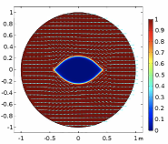
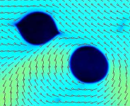
In Fig. 1, we present an example of experimental nematic/isotropic configuration obtained in the laboratory of Oleg Lavrentovich along with a figure showing a numerically generated phase boundary based on gradient flow for . Both figures represent transient states but we point out the similar nature of the singular phase boundaries. Note that in the experimental picture, the phase boundary is singular only for the isotropic island whose surrounding nematic phase has degree on the boundary of the isotropic tactoid, not for the island where the degree is . This distinction will come up frequently in our analysis.
Regarding a rigorous identification of the -limit of , we only have partial results at this point. We present rigorous compactness results in in Theorem 3.4 based on an adaptation of [12], but roughly put, it is easy to verify that any limit of an energy bounded sequence, i.e. such that , is a vector field such that the isotropic phase is a set of finite perimeter. Then making the extra assumption that is of bounded variation in the nematic phase where , one can invoke a combination of known techniques [17, 34] to establish a lower bound on the limit of the form
| (1.7) |
where is the standard Modica-Mortola cost of an interface, cf. (2.6), and is a wall cost, arising through an abstractly defined solution to a certain cell problem. We wish to emphasize that, unlike for example (1.1), the limiting problem that arises involves both interfacial energy terms and a bulk term.
We strongly suspect that this wall cost is in fact the cost associated with the heteroclinic connection between the states and where is the approximate tangent to the jump set, see (3.8) and (3.9). The upper bound based on a recovery sequence for such a “one-dimensional” wall where only the tangential component varies across the boundary layer is the content of Theorem 3.1.
The optimality of one-dimensional walls is a delicate point that turns out to hold in the analysis of (1.2)-(1.3), cf. [17], as well as in the analysis of the divergence-free, or equivalently , versions of these problems known as the Aviles-Giga problem, see e.g. [3, 5, 9, 12, 18, 25, 26, 33, 34]. However, for Aviles-Giga and in [17], the matching of lower bound to upper bound is achieved through the somewhat miraculous Jin-Kohn entropy, cf. [20] and (3.13). The divergence of this vector field on the one hand bounds the Aviles-Giga energy from below but at the same time yields a value for the cost of a wall that coincides with the one-dimensional upper bound construction described above. As far as we can tell, there is no analogous entropy that works similarly for (1.5).
In Section 3.3, in contrast to the partial results from Section 3.1, we establish a complete -convergence analysis along with optimal compactness, in the case where is an interval.
In Section 3.4, we turn to the derivation of criticality conditions for the proposed -limit, . As in [17], we find that in the -valued phase, away from walls, we can phrase criticality in terms of a system of conservation laws sharing characteristics, cf. Corollary 3.11. Characteristics turn out to be circular arcs along which divergence is constant with the curvature of the arc being given by the value of the divergence. We also explore criticality conditions for the wall and interface in Theorems 3.9 and 3.12, as well as for possible junctions between walls and interfaces in Theorem 3.13, whose somewhat technical proof we delay until the appendix.
Section 4 is crucial to our paper in that we explore the possible morphology of vortices, interfaces and walls through a series of examples. We focus on constructing critical points to the formal limit of which one might describe as the Aviles-Giga -limit augmented by isotropic regions, see (4.1). These constructions are in particular divergence-free competitors for for finite that should be close to optimal for large. One might expect that when no area constraint on the size of the isotropic phase is imposed and -valued Dirichlet data is specified in (1.6) for , then only critical points that are nematic–i.e. -valued– would emerge, with perhaps a certain number of defects in order to accommodate the degree of , as in [8]. However, in Example 4.3, we take to be the unit disk and to have negative degree, and we show that, somewhat surprisingly, an isotropic region opens up. We provide a possible explanation for this phenomenon in Theorem 4.1.
In Section 4.4, we construct a divergence-free example in all of in which a singular phase boundary encloses an isotropic island and in which the infinite nematic complement of this island obeys a trivial degree zero condition at infinity, i.e. as . Unlike in the first example, this island is induced through an area constraint. This somewhat delicate calculation involves construction of both interfaces and walls with proper junction conditions holding at their intersection.
In this section we also comment on the following crucial feature of the model observed in several of our examples. At defects on the phase boundary, the director often switches the sense of tangency. If a defect is a corner in the interior of the domain and a change in tangency occurs, then walls necessarily emanate from the defect in order to avoid infinite energy from the bulk divergence term; see Fig. 4 and the discussions at the end of Section 4.2 and preceding Example 4.4 .
Needless to say, this article represents just the initial investigation of a problem which holds within it a rich array of phenomena yet to be understood and questions to be pursued. We also mention that upgrading this model to the setting of -tensors should not pose significant obstacles.
2 First try: A model whose elastic disparity is weak
In this section, we begin our examination of the effect of disparity in elastic energy. Throughout this section, we will consider a continuous potential which vanishes on . We assume that for some continuous function , one has with then and elsewhere. The prototype for what we have in mind is the Chern-Simons-Higgs potential
| (2.1) |
Then for a sequence of positive numbers we consider the sequence of functionals
| (2.5) |
Though the -convergence result below holds for any sequence approaching zero, we are especially interested in the situation where
so that the divergence term in the elastic energy is heavily emphasized. Our goal is to explore whether or not this disparity can produce a -limit whose minimizers possess the types of phase boundary singularities reminiscent of isotropic-nematic interfaces as described in the introduction. What we shall find is that this level of elastic disparity is in fact not sufficiently strong to achieve this goal.
To this end, we define our candidate for the -limit:
Here,
| (2.6) |
The reader may well recognize this -limit as precisely the well-known limit of the Modica-Mortola energies, an indication that to leading order in the energy, the divergence term has no effect on the asymptotic behavior of minimizers.
Our main result for this section is:
Theorem 2.1.
The sequence -converges to in the topology induced by the norm of the modulus . That is,
-
(i)
for any and for any sequence in ,
(2.7) and
-
(ii)
for each there exists a recovery sequence in satisfying
(2.8) In fact, we can construct the sequence so that in .
Remark 2.2.
Regarding the asymptotic behavior of global minimizers, this result does not seem to address the possibility of a phase transition since there is no ‘incentive’ for a minimizer of to take on both and values. To encourage a phase transition for a minimizer, one could, for example, impose a mass constraint such as
Alternatively, one could impose a Dirichlet condition on such as where is -valued on one portion of the boundary and then transitions smoothly down to on the rest of the boundary. Either of these alterations in the problem can be easily accommodated using what are by now standard techniques in -convergence, see e.g. [27, 32, 37]. However, in order to present the main ideas without excessive technicalities, we formulate and prove a -convergence theorem without either of these conditions, and merely remark that they could be incorporated if desired.
Though as indicated below (2.8), we can in fact establish -convergence in the stronger topology , it is not possible to obtain -compactness for an arbitrary energy bounded sequence due to the degeneracy of the well . However, -compactness of follows by a standard argument, cf. e.g. [37, Proposition 3].
Proposition 2.3.
Let be a sequence of maps from to and assume that the sequence of energies is uniformly bounded. Then there exists a subsequence and such that in .
As observed in [31], this rather weak form of compactness is nonetheless sufficient to imply the existence of local minimizers of given a local minimizer of which is isolated in this weaker topology, by modifying an argument of [22]. For example, on a “dumbbell”-type domain, there always exist local minimizers of for sufficiently small, cf. [31, Theorems 4.2, 5.1].
Proof of the lower semi-continuity condition (2.7).
Lower semi-continuity follows as in the Modica-Mortola setting since one simply ignores the divergence term. Since the argument is short, however, we present it here. The cases in which or on a set of positive measure are trivial. We therefore assume that , and suppose that in Suppose also for now that an assertion we will justify later by means of a truncation procedure. In the argument below, we will make use of the function As we have
By the assumption that we obtain a uniform bound on in , implying the existence of a subsequence converging in to . Therefore, by lower semi-continuity in ,
This then completes the proof of (2.7) under the assumption that
If it does not hold that then we define
We compute that
| (2.9) |
Finally, we have that
so that we can combine the previous arguments with (2.9) to obtain lower semi-continuity for the original sequence . ∎
Proof of the recovery sequence condition (2.8).
Suppose we are given with We will construct a sequence with in such that . We first briefly discuss the main idea, in order to motivate the construction that follows. Suppose that is smooth on the set, say , where it is -valued, except for finitely many singular points , and suppose carries degree around each “vortex” . Suppose also that is smooth. We would like to define using a boundary layer near which bridges the values of near to outside. In order to recover the correct -limit with constant , we must define on a neighborhoods of so that
As this is the least upper bound we could achieve even if , we must therefore construct on so that
and so that the gradient squared and potential terms give the correct asymptotic limit. Since there is no assumption on how fast the sequence approaches zero, a natural construction to try is to define on so that it is divergence-free there. This can be done by setting
| (2.10) |
where is the distance function to and is a suitably defined scalar function bridging the values and . Then
| (2.11) |
It is easy to check that if is a smooth, non-zero vector field tangent to level sets of , as above, then its degree restricted to such a level set is . If, however, , then degree considerations imply that it is impossible to define smooth which are non-zero and tangent to but equal to in the interior of away from the boundary. In addition, even if , defining inside by mollifying could yield vortices which result in unbounded energy as ; see Theorem 4.1.
To address these issues, it is instructive to consider the case in which is the ball of radius centered at the origin, is the unit disk with there and vanishes on the annulus . As explained above, there is no smooth field tangent to the boundary of the disk and equal to inside the disk. However, suppose we alter the boundary of the disk by adding two small cusps. Then we can define a continuous vector field tangent to the modified boundary, except at the cusps, which has degree zero. This tangent vector field allows for the construction of a boundary layer similar to (2.10) which contributes a perimeter term differing from by a negligible amount, and a second, -valued boundary layer inside the disk which bridges the degree zero tangent field to the constant . The energetic contribution of this second layer vanishes in the limit.
Our general construction utilizes this basic idea. Given any component of the nematic region , we first approximate there by a map with degree zero around any closed curve lying in that component. This allows us to avoid the creation of vortices which are energetically too expensive for the divergence term. Then, we add two cusps to the boundary components of the nematic regions; and finally, we use two boundary layers to bridge to the values in the nematic regions. We should emphasize that the approximations will be close to the original function in but of course will not be close in a stronger topology as that would violate basic properties of degree.
We now fix any such that and begin our construction of the recovery sequence. We first approximate by vector fields , then construct a recovery sequence for any . A standard diagonal procedure will then imply the existence of a recovery sequence for . We begin by showing that there exists an intermediate sequence of vector fields such that
-
(i)
has boundary,
-
(ii)
is smooth restricted to ,
-
(iii)
for each , there exists a non-empty arc such that for all ,
-
(iv)
where denotes one-dimensional Hausdorff measure,
-
(v)
in , and
-
(vi)
.
It is standard that there exist such that , , and hold and in , see e.g. [16, Theorem 1.24]. Next, we define a sequence by
The choice of is arbitrary, since any unit vector would suffice. From the convergence of to and the dominated convergence theorem, it follows that, up to a subsequence, in . The sequence satisfies properties and –, so it remains to argue we can modify it so that and hold as well. For each , we define for
and observe that for some , , since . Then for , we redefine to be identically , so that the now avoids an arc of length . Now we can mollify to obtain smooth which also avoid and satisfy –. Indeed, this can be done by choosing an interval in which to define the values of the phase of and mollifying the phase function itself. We also point out that inside , the degree of around any simple, closed curve is zero, since cannot take values in .
Next, for each , we add small cusps to the sets and modify to obtain . For each connected component of , we add two cusps pointing into the isotropic region, which change the perimeter of by at most . We denote the resulting modification of by , and smoothly alter the values of the function , yielding . This procedure can be carried out in such a fashion so that properties – above still hold for the sequence , and property , the smoothness of , holds except at the cusps. This completes the construction of the sequence .
For each , we now construct a recovery sequence , suppressing the dependence of on for ease of notation. Away from , will be identically equal to . Near , we will use a boundary layer of the form , where is a unit vector field tangent to level sets of the signed distance function to and where solves a certain ODE. Away from the cusps, the level sets of the are smooth, which will be enough for our purposes. For each connected component of , we define there by choosing a unit vector field tangent to that component and continuous on all of that component; see Fig. LABEL:Fig._1 below.
The fact that each component contains two cusps implies that for the field to be continuous, it must change the sense of tangency at every cusp. Thus on , is always equal to . From these observations it follows that the degree of around any connected component of is zero. We then extend to a continuous, unit vector field tangent to level sets of for such that is small and positive and the nearest point projection onto is not contained in any one of a union of rectangles near each cusp; see Fig. LABEL:Fig._2 below. To bridge the divergence free field to the values of inside , there is a second boundary layer, which is defined via an -valued homotopy between and the values of inside . This is only possible because has degree zero around , as does around any simple, closed curve in . The energy contribution from this layer in the limit will be zero, since there.
We now specify in the first boundary layer, which contributes the perimeter term in the asymptotic limit. In the interior of and in at sufficient distances away from to be specified shortly, we set equal to .
First, for some fixed , we consider the following ODE, similar to [6, Equation 3.2]:
As argued in [6], there exists a constant , depending on , such that for every , there exist positive numbers and strictly decreasing solutions of this ODE such that
| (2.12) |
and
Each in fact depends on , but we suppress this dependence. Next, we excise a small rectangle at each cusp. Let
| (2.13) |
For each cusp , consider a rectangle with one side of length , centered at , and perpendicular to the one-sided tangents at , such that protrudes into the isotropic set in the other direction; see Fig. LABEL:Fig._2 below. We denote by the union of all ’s and then we define
In the definition above and in the remainder of the argument, we take to denote the signed distance function to which is negative inside . We will deal with on and on at the end. It can be shown, by calculations similar to those preceding [31, Equation 3.33] that
| (2.14) |
observing in the process the crucial fact that the divergence of on this set is zero, cf. (2.11). Furthermore,
| (2.15) | ||||
since and and are bounded functions independent of away from .
It remains to define on the second boundary layer, , and on . Let us first consider the second boundary layer. Because of the fact that defined thus far has degree zero around and , there exist Lipschitz phases , such that on and on . Then we can interpolate on the intermediate region using convex combinations of and so that and are both . Since is a unit vector field here, is . Hence we can calculate
| (2.16) |
So on the second boundary layer contributes nothing to the asymptotic limit.
Finally, we treat on the union of rectangles . It suffices to demonstrate the construction on a single such that the cusp contained on one of its sides is the origin and the isotropic phase is to the right of the -axis. Up to a translation, this is the situation depicted in Fig. LABEL:Fig._2 with . In these coordinates we may describe as the rectangle . We set
on , which ensures compatibility with as previously defined. We remark that is either plus or minus . Then on , , and . Since the area of is by (2.12) and (2.13), we have for small
| (2.17) |
Combining (2.14)–(2.17), we obtain
In addition, the converge in to by virtue of the dominated convergence theorem, since they are bounded and the set where they differ from has measure going to zero. Therefore, recalling that depends on as well, we diagonalize over and to obtain a recovery sequence for . Since converge in to and , a second diagonalization argument over and yields a recovery sequence for . ∎
3 A model with large elastic disparity and singular phase boundaries
In the previous section we saw that disparity in the elastic energy density of the form
is insufficient to induce a singular phase boundary between the isotropic state and an -valued nematic state in minimizers of the -limit. We now introduce a model with still larger disparity, and it is this model we will work with for the remainder of the article.
To this end, for a positive constant independent of we define
| (3.1) |
where for some continuous that vanishes only at and . As always, our prototype is the potential given by , but in what follows we can allow for more general potentials vanishing at and , provided that for some constant one has the condition
| (3.2) |
for any .
In light of the divergence term in , it is clear that energy-bounded sequences will have divergences that converge weakly in As we will discuss in Section 3.3, under the assumption (3.2), an adaptation of the compactness techniques of [12] allows us to also establish that a subsequence of will converge strongly in to a limit taking values in . We will write when both weakly in and strongly in . See Theorem 3.4.
These compactness results naturally lead us to consider the Hilbert space of vector fields having divergence, and more specifically , in light of the assumed zero set of the potential .
A vector field that additionally lies in the space is known to have a countably -rectifiable jump set off of which is approximately continuous. In our pursuit of a possible candidate for the limit of the sequence we will focus on functions lying in the intersection of these two spaces.
Mappings in have well-defined traces, say and on either side of and an easy application of the Divergence Theorem reveals that when vector fields have jump discontinuities across then necessarily the normal component is continuous, i.e.
| (3.3) |
where is the (approximate) normal to .
This brings us to a crucial distinction when attempting to identify a limiting energy for the sequence –a mapping may undergo a jump between two -valued states, in which case (3.3) is supplemented by the additional requirement that
| (3.4) |
where is the approximate tangent to . We will refer to any component of bridging two -valued states as a wall. On the other hand, may jump between an -valued state, say , and , in which case (3.3) implies that must coincide with . We will refer to any such component of as an interface. It is this tangency requirement along an interface that can induce singularities in the isotropic-nematic phase boundary.
3.1 A conjecture for the -limit of
Our goal in this section is to make the case for a proposed -limit of the sequence defined in (3.1). While we do not at present have matching upper and lower asymptotic bounds for this sequence, we do have a construction leading to an asymptotic upper bound which we strongly suspect is sharp. We will begin with a description of this construction and then discuss various strategies for lower bounds, why the analogue of what works for the Ginzburg-Landau potential, cf. [17], apparently fails here and what the evidence is to support our conjecture on the sharpness of the upper bound.
We should say at the outset that our pursuit of the -limit begins with the assumption that . While this is not the natural space from the standpoint of compactness, the identification of the correct limiting space is non-trivial and we do not attempt to address it here. We refer the reader to [3, 10, 24] for more discussion of this issue. We make the assumption here in order to speak sensibly about the -rectifiability of the jump set , though for that part of corresponding to interfaces, i.e. to , as we will note below, this rectifiability comes easily from the fact that limits of energy-bounded sequences satisfy
As noted above, for such a vector-valued function , the jump set naturally splits into two types: walls and interfaces, though these two types of singular curves may well meet in junctions, see e.g. Theorem 3.13 and Fig. LABEL:Junctionfig. An upper bound construction then rests on efficiently smoothing out these jump discontinuities, and in both cases, we rely on a one-dimensional type of resolution described formally below. The rigorous execution of these ideas follows the approach of [9] as adapted in [17].
To resolve an interface separating an isotropic region where from a nematic region where we invoke a by-now standard Modica-Mortola type of heteroclinic connection in the modulus. More precisely, after mollifying the interface to smoothen it if necessary, we mollify in the nematic region and make a boundary layer construction, say , of the form
| (3.5) |
where denotes the signed distance function to and where minimizes the d energy
| (3.6) |
This leads to the same ‘interfacial cost’ encountered in Section 2, namely
multiplying the perimeter of the interface. Since
the term in will contribute nothing to such a boundary layer construction in the limit since the first term is controlled by the fact that and the second term is negligible due to the required tangency of and along an interface. We note that the ansatz (3.5) would fail for the sequence of functionals analyzed in Section 2 since there is not required to lie in and so the term will in general not vanish.
With appropriate care taken to treat issues of regularity, this can be made rigorous. What is more, this construction, based only on appropriate interpolation of the modulus between and , gives a sharp upper bound on the interfacial energy, in light of the inequality
| (3.7) |
Since this is the classical scalar Modica-Mortola functional in terms of the function , when applied in a neighborhood of the interface it yields the matching lower bound of
Our boundary layer construction in a neighborhood of a wall separating two -valued states, say and , is one-dimensional in a different sense. In light of the continuity of the normal component of across a wall, cf. (3.3), a natural choice is to fix the value of across the boundary layer and use a heteroclinic connection to bridge the value of to , that is, to bridge to in light of (3.4).
At a point on the wall, such a choice leads to a cost per unit length given by the minimum of a heteroclinic connection problem that is a bit different from (3.6), namely
taken over such that
One easily checks that this infimum is given by where we define
| (3.8) |
which in the prototypical case of takes the form
| (3.9) |
We point out that and also note that is not a monotone function of on , but rather increases to a unique maximum and then decreases down to zero at .
Such an upper bound construction leads us to our conjectured -limit when , namely given by
| (3.10) |
One should also impose upon competitors in the minimization of a boundary condition of the form (1.6) if one imposes the Dirichlet condition for or an area constraint on the measure of the isotropic or nematic region within if an integral constraint has been imposed on .
In particular, we can rigorously assert:
Theorem 3.1.
For any , there exists a sequence with such that
| (3.11) |
Furthermore, we state a conjecture:
Conjecture : Suppose satisfies (3.2). Then for any and any sequence we have
| (3.12) |
Proof.
The proof of (3.11) is similar to the proof of [17, Theorem 3.2(ii)], which itself is an adaptation of the techniques laid out in [9] for Aviles-Giga recovery sequences, so we omit the details. The only difference between the arugment here and the argument in [17] is that, as discussed above, in addition to walls, there are also interfaces now in which jumps from a tangent -valued state to . However, this does not pose a serious obstacle to the construction, as the important technical components are the rectifiability of the jump set and the condition (3.3) satisfied along at either a wall or interface, which goes to guarantee that the boundary layer constructions do not contribute asymptotically to the -norm of the divergence. ∎
Remark 3.2.
We have not addressed in (3.10) or in Theorem 3.1 the issue of boundary conditions, so we describe now how to incorporate them. Suppose one were to fix Dirichlet data for admissible functions in . The functions could be -valued, or could transition smoothly between and if we are trying to induce a phase transition. Let us assume that in for some . We observe that for a sequence satisfying on and so in particular , under the convergence with , it follows from the divergence theorem and the convergence of to that
In this case, the limiting energy would also contain integrals around the portion of where , and the cost along these portions would either be given by or .
Remark 3.3.
An a priori sharper upper bound for the wall cost could be obtained for these energies using the techniques of [33]. There, the author obtains an upper bound without assuming that the optimal profile is one-dimensional. Instead, the cost is defined via a cell problem. As the class of admissible functions for the cell problem is strictly larger than the class of d competitors, the cell problem yields what could in theory be a sharper upper bound. However, since we conjecture that the one-dimensional profile is optimal and since at present we see no way to analyze the abstract cell problem to make this comparison, we do not pursue the strategy from [33].
Given the presence of arguments leading to matching lower bounds for one-dimensional constructions in the Aviles-Giga problem [5] and for the energy with the potential replaced by a Ginzburg-Landau potential , in [17], it behooves us to comment on why, at present, we have no such argument here. In [5] and in [17], the authors employ the celebrated Jin-Kohn entropy [20]. Defining
| (3.13) |
the version of these entropies well-suited to the situation where the jump set is parallel to one of the coordinate axes, one can then calculate
| (3.14) |
In the divergence-free Aviles-Giga setting of [20], the last term drops out and an application of the inequality allows one to bound the Aviles-Giga energy density from below by . When the divergence is possibly non-zero, as in [17], a slight modification yields
which is the crux of the argument.
Unfortunately, for most radial potentials that are not the Ginzburg-Landau potential , this technique does not seem to work. First, we note that
where the integrands are, up to signs, given by . Therefore, to obtain a version of (3.14) with replaced by , where is our potential vanishing on , the natural choice for the vector field to replace would be
When we calculate the divergence of , we get
The only way for to factor out of the last two terms is if
which holds for radial when is linear in . This cannot hold for any that vanishes only at and .
We point out that a related problem that has resisted resolution for several decades is the determination of a sharp lower bound for the sequence of energies
| (3.15) |
where competitors must be divergence-free. Here too it is conjectured that the optimal lower bound for the wall cost is based on a one-dimensional ansatz, [3], but a proof has not been found, and in particular, no version of the Jin-Kohn entropy is evident. An abstract lower bound involving a cell problem for functionals of this type has been derived in [34], but has not yet to our knowledge been matched by a corresponding upper bound. The strategy in this and other papers involving a lower bound phrased in terms of a cell problem is based on a blow up procedure introduced in [15]. Such a lower bound of the form for some defined as the solution to a cell problem could be derived for our wall energy as well, but we do not include the argument since it does not provide much insight here.
On the other hand, for in (3.15), as shown in [3], the one-dimensional ansatz is not optimal, with an oscillatory construction, often referred to as ‘microstructure,’ whose modulus hews close to , yielding a lower asymptotic energy.
So what is the rationale behind our conjecture (3.12)? One key point is that for given by or more generally by a potential satisfying (3.2), the level of degeneracy of the potential well is no flatter than that of where again it is known that walls follow a one-dimensional profile asymptotically. Thus, it seems unlikely that microstructure of the type emerging, for example, in (3.15) for would appear here since for our model it is no more beneficial energetically to abandon one-dimensionality in order to be nearer to across a wall than it was in (1.2).
Other evidence for our conjecture is numerical. Repeated numerical experiments in the form of gradient flow for with small in a variety of domains, for a variety of boundary conditions and for a wide range of values have not indicated any lack of one-dimensionality in the wall structure. Were the transition to be truly , one might expect the wall to exhibit some oscillation or other instability. For example, in [17] while we prove that for (1.2)-(1.3) the wall cost is based on a one-dimensional construction, we also find that when minimizing (1.2) in a rectangle with -valued Dirichlet data given by for on the top and bottom respectively and periodic boundary conditions on the sides, there exists a parameter regime in and in the box dimensions where the minimizer is not one-dimensional, cf. [17], Thm. 6.6. Indeed this theorem is supported by numerics revealing the eventual instability of a horizontal wall and the emergence of so-called ‘cross-ties’ commonly arising in studies of micromagnetics such as [2]. On the other hand, as we discuss in Section 4.1, numerically we detect no such instability of a horizontal wall for under these boundary conditions. Then a numerical examination in Section 4.3 of wall structure for a version of our problem posed in a disk also indicates a one-dimensional heteroclinic connection for the wall structure. This gives us further confidence in the conjectured one-dimensionality of the wall cost.
3.2 Compactness
In this section we establish a compactness result for energy-bounded sequences. Recalling the assumption (3.2), we begin by observing that
| (3.16) |
Both the Ginzburg-Landau and the Chern-Simons-Higgs potentials satisfy this inequality and in [17] it is shown that for given by the Ginzburg-Landau potential, the compactness result of [12] generalizes to . In this section, we show that this compactness approach generalizes to potentials also vanishing at the origin provided we assume (3.2).
Theorem 3.4.
Let be a sequence such , with independent of . Then there exists a subsequence (still denoted here by ) and a function with such that
| (3.17) | |||
| (3.18) |
The fact that for a subsequence of , one has in where follows from inequality (3.7) via the standard Modica-Mortola approach, cf. [27] or [37]. The proof of (3.17) follows immediately from the uniform bound on the norm of the divergences, so we turn to the proof of (3.18). The proof follows closely the proof in [12, Proposition 1.2], with the details suitably modified to account for the fact that the potential may now possibly vanish at in addition to . Below we outline the procedure and indicate which portions require changes from [12].
The proof relies on compensated compactness and a careful analysis of the Young measure generated by the sequence . One of the key tools in this analysis is the concept of an entropy, defined here as a mapping such that
where , cf. [12, Definition 2.1]. A crucial property of any such entropy is that satisfies a certain equation relating and for any . We state this equation precisely in (3.2), and refer the reader to [12, Lemmas 2.2, 2.3] for the proof, which is a straightforward calculation. In Lemma 3.5, we prove that the class of entropies is large enough for our purposes. Next, in Proposition 3.7, we prove the requisite compactness for the sequence . We achieve this by first adapting the proof of [12, Proposition 1.2] using the aforementioned equation (3.2) to show that for any entropy ,
This compactness then allows us to use the div-curl lemma of Murat and Tartar [29, 38] and the result of Lemma 3.5 to conclude that each is a Dirac measure. One can then quickly deduce, in the same fashion as in [12, page 843], that the sequence is precompact is . We begin the proof with
Lemma 3.5.
(cf. [12, Lemma 2.2]) Let be a probability measure on supported on . Suppose it has the property
| (3.19) |
Then is a Dirac measure.
Remark 3.6.
We point out that the proof of this lemma does not generalize to the case where the potential vanishes on a pair of circles that both have non-zero radius. As a consequence, this proof of Theorem 3.4 does not generalize to such situations.
Proof.
We begin by recalling the definition of “generalized entropy” from [12, Lemma 2.5]. These are functions defined by
| (3.22) |
for any fixed . Any such can be approximated closely enough by entropies such that (3.19) holds for as well. Using the fact that these generalized entropies vanish at the origin, we have
We rewrite this as
or
Letting approach , we obtain
or
| (3.23) |
If then it cannot be that for any . In this case for all -valued , and is clearly a Dirac measure concentrated at zero. So we may assume that , implying that is a probability measure on . In this case, we deduce from (3.23) that
As is a probability measure on , this implies that is concentrated on a single point. ∎
We can now prove the main result.
Proposition 3.7.
(cf. [12, Proposition 1.2]) Let be open and bounded. Let be such that
| (3.24) |
| (3.25) |
and
| (3.26) |
Then
| (3.27) |
Proof.
First, we modify our sequence slightly for convenience. By choosing real numbers close enough to and considering the sequence , we can without loss of generality assume that for each ,
| (3.28) |
In addition, we can choose so that has uniformly bounded energies and is precompact in if and only if is as well. Henceforth we refer to the modified sequence as simply and assume that these conditions hold for .
We aim to show for any entropy that
| (3.29) |
Utilizing (3.24), (3.28) and [12, Lemmas 2.2, 2.3], we see that there exists and such that at a.e. point in one has
Before proceeding, we let denote a smooth, increasing, bounded function with bounded derivative such that for and for . We will utilize the sequence , and we remark that could readily be replaced by any number less than . Replacing by as such allows us to maintain control on as opposed to having to analyze the distributional gradient of a sgn function, as will be necessary in a step at the end of the proof. Continuing from (3.2), we find that
| (3.30) | |||
| (3.31) |
We claim the remainder terms are bounded uniformly in . Noticing that if , we have
Continuing now using Holder’s inequality and the bound , we have
To prove (3.29), we will prove that the sequence
| (3.32) |
Since the energy bound implies that converges to in , the divergence of this sequence converges to in . Thus (3.32) implies (3.29). Thanks to (3.30), we have that
We will show the desired compactness by appealing to a lemma of [30], cf. [12, Lemma 3.1]. This entails verifying the following two claims:
(1) The sequence is uniformly bounded in
(2) The sequence is uniformly integrable.
Proof of (1): We have shown that the are uniformly bounded in and the boundedness of the function along with the bound on yield that is uniformly bounded in It remains to show that the last term, namely , is bounded in We have
The desired bound follows from Cauchy-Schwarz along with the energy bound.
Proof of (2): This is clear from the fact that , , , and are bounded functions.
We have now proved that is compact in . The rest of the proof follows as in the second step of [12, Propositon 1.2]. ∎
3.3 The -limit of among 1d competitors
In this section we analyze -convergence of where competitors are defined on an interval for some and are required to satisfy -valued boundary conditions of the form
| (3.33) |
Under the one-dimensional assumption, takes the form
| (3.37) |
In a manner similar to [17], Section 6, within this one-dimensional ansatz we can obtain a sharp compactness theorem for energy bounded sequences, a complete convergence result of the functionals and a complete characterization of minimizers of the -limit. Since the proofs of the results in this section are completely analogous to those in [17, Section 6], we only sketch the arguments highlighting differences.
In Section 4.1, we present results of numerical simulations obtained via gradient flow for with for the two-dimensional problem in a rectangle , subject to the boundary conditions (3.33) on the top and bottom and periodic boundary conditions on the left and right sides. These computations suggest convergence in large time to configurations that resemble the one-dimensional minimizers of this section, lending further evidence to our conjecture (3.12). We emphasize that the initial data for these numerics were not restricted to be one-dimensional.
We continue making the assumption (3.2) on our potentials. Recall that we are writing . We begin with a compactness result.
Theorem 3.8.
Let with . Then there exists with
such that up to a subsequence, in . In addition, , in for all , and
Proof.
Throughout the course of the proof, we repeatedly pass to further and further subsequences of converging to zero but suppress this from our notation. We notice that thanks to the uniform bound from (3.2), after passing to a subsequence,
| (3.38) |
Furthermore, this bound, along with the uniform bound on yields after passing to a further subsequence that
| (3.39) |
Finally, from the bound on the potential, there exists such that
| (3.40) |
It remains to upgrade the convergence of from weak to strong convergence. An algebraic identity is used in the proof of [17, Theorem 6.1] to obtain strong convergence. Here, without an explicit expression for we proceed differently. As in [17], we utilize the “entropy ” defined by
| (3.41) |
We set , so that
| (3.42) |
On the one hand,
| (3.43) |
On the other hand, using (3.2) and a Cauchy-Schwarz argument completely analogous to that found in [17], we note that is bounded in . Upon passing to a subsequence, we conclude that converges in and upon passing to a further subsequence, converges almost everywhere. Consequently, using (3.42) and (3.43), we find that converges almost everywhere as well.
Finally, since and strongly in , we can apply the Lebesgue dominated convergence theorem to conclude that converges strongly in to some limit. From (3.38), this limit is and it follows that or a.e. and that the limit of is . Since is when , we see that , which concludes the proof. ∎
We turn next to -convergence in this one-dimensional setting. The analogue of from (3.10) is the energy
| (3.44) |
One can establish the -convergence of to in a completely analogous manner to the proof of Theorem 6.2 in [17], so we omit the details.
Finally, as in Theorem 6.4 of [17], and with identical proofs, one can characterize the minimizers of (3.44) explicitly. When the boundary conditions (3.33) are different from the minimizer is unique and consists of a single wall occuring at , no interfaces and bulk contribution in the regions : the function is piecewise linear and jumps from to across . The optimal jump value is easily determined by optimizing over the bulk and jump contributions. Finally when the Dirichlet boundary conditions on the top and the bottom are given by we find two parameter regimes similar to the situation in [17]. When is smaller than a certain threshold, the minimizer is unique and has both bulk divergence and jump contributions. However for larger values, the minimizer only has perimeter contribution, along with two interfaces, one connecting to and the other connecting to These interfaces divide the interval into subintervals in each of which the minimizer is a constant. See Section 4.1 for numerical simulations.
3.4 Criticality conditions for
In this section we will describe criticality conditions associated with critical points of the conjectured -limit given by (3.10). For , we recall the notation , with given by (3.8) or (3.9) in the case of the Chern-Simons-Higgs potential, for the cost per arclength of a jump from one -valued state, say to another one, say across a jump set , with denoting the unit normal pointing from the side of a wall to the side. We recall that for such a jump, an vector field must satisfy the requirement
| (3.45) |
In light of (3.45), we will sometimes write just when evaluating the normal component of along .
We also recall that for portions of corresponding to a jump from the isotropic state to an -valued state , the cost per unit arclength is given by and condition (3.45) becomes simply .
Parts of the argument follow the same lines as in the proof of Theorem 4.1 in [17] except that the cost in that paper is the one associated with a Ginzburg-Landau potential, namely where
which can also be written as or equivalently
However, in the present context, we will need to distinguish between variations of the ‘walls’ separating two -valued states and ‘interfaces’ separating the isotropic state from an -valued state. We will also examine criticality conditions at a junction corresponding to the intersection of these two kinds of curves. We begin with:
Theorem 3.9.
(Variations that fix the jump set)
Consider any such that on . Denote by its jump set. Then if the first variation of evaluated at vanishes when taken with respect to perturbations compactly supported in , one has the condition
| (3.46) |
where .
Now assume the first variation vanishes at when taken with respect to perturbations that fix and are supported within any ball centered at a smooth point of . If separates the ball into two regions where is given by -valued states and and if the traces and are sufficiently smooth, then one has the condition
| (3.47) |
where represents the jump in divergence across and is the unit normal to pointing from region to region .
Remark 3.10.
There is no natural boundary condition analogous to (3.47) for such variations taken about a point of where separates an isotropic state from an -valued state since the requirement of tangency in such a configuration is too rigid to allow for a rich enough class of perturbations.
Proof.
To derive conditions (3.46) and (3.47) we assume that for some point and for some , either
or else and the following conditions hold :
(i) The set is a smooth curve, which we denote by and which admits a smooth parametrization by arclength, which we denote by for some with
(ii) On either side of the critical point and possess smooth traces on . We will denote the two components of by and and we denote on these two sets by , for .
We will present the argument for case (ii), indicating how the easier case (i) follows from the same analysis.
To define an allowable perturbation of the critical point given by and , we must maintain the property of being -valued, so to that end we introduce smooth functions for some such that the perturbations of and take the form
| (3.48) |
shifting just for the moment to complex notation. Introducing , expanding (3.48) and reverting back to an -valued description of we find that for one has
| (3.49) |
Along , we must also be sure to preserve to the condition (3.45), namely
| (3.50) |
Invoking (3.45) for the unperturbed critical point, along with (3.49) we find that to provided
However, since
| (3.51) |
along the jump set bridging -valued states, it follows that we must require
| (3.52) |
For later use, we also record that from (3.49) and (3.51) one has along the expansion
| (3.53) |
Now we calculate
Taking the -derivatives and evaluating at we obtain
Integrating by parts, a vanishing first variation of this type leads to the condition
| (3.54) |
Corollary 3.11.
(cf. [17], Cor. 4.2). Suppose is smooth and critical for in the sense of (3.46). Then writing locally in terms of a lifting as and defining the scalar one has that (3.46) is equivalent to the following system for the two scalars and :
| (3.55) | |||
| (3.56) |
Consequently, starting from any initial curve in parametrized via along which and take values
and respectively, the characteristic curves, say
, are given by
| (3.57) | |||
| (3.58) |
whenever The corresponding solutions and are given by
| (3.59) |
so that the characteristics are circular arcs of curvature and carry constant values of the divergence. In case the divergence vanishes somewhere along the initial curve, i.e. , then the characteristic is a straight line.
We also consider the implications of criticality with respect to perturbations of the jump set itself.
Theorem 3.12.
(Variations of the jump set)
Under the same assumptions on as in the previous theorem, suppose in addition to the criticality with respect to perturbations that fix the location of , one also assumes the
vanishing of the first variation of evaluated at , allowing for local perturbations of the jump set itself. Then along any points of where jumps between two -valued maps and , a vanishing first variation leads to the condition
| (3.60) |
at any point such that , and are sufficiently smooth in some ball centered at . Here denotes the curvature of , denotes the unit tangent to and is the unit normal to pointing from the side of to the side. The notation refers to the tangential derivative along the jump set.
For portions of separating an -valued state from the isotropic state , criticality takes the form
| (3.61) |
where is a Lagrange multiplier that is present only if is considered subject to an area constraint on the measure of the isotropic phase . Also, since requires that along such a portion of , we note that in (3.61) one either has or .
Proof.
To derive condition (3.60) assume that for some point the following conditions hold in a ball for some radius :
(i) The set is a smooth curve, which we denote by and which admits a smooth parametrization by arclength, which we denote by for some with
(ii) On either side of the critical point is with traces on . We will denote the two components of by and and we denote on these two sets by , for .
Again, our convention for the unit normal is that it points out of into .
For the calculation it will be convenient to assume that for , has been smoothly extended so as to be defined in an open neighborhood of . We take this extension to be executed so that is constant along and so that is constant along .
In order to effect a smooth perturbation of , and we now introduce a vector field . For convenience we will assume that is parallel to for and so we introduce the scalar function such that
| (3.62) |
where . Here we have written for the composition Then let solve
| (3.63) |
for some . Expanding in we find that
| (3.64) |
so that in particular one has the identity
| (3.65) |
Throughout this proof, the symbol refers to an equivalence up to terms that are .
Now we define the evolution of the curve via the vector field by with corresponding parametrization
| (3.66) |
in light of (3.62). A simple calculation goes to show that the normal to takes the form
| (3.67) |
where we have introduce the notation for the unit tangent to . We caution that the parameter used to parametrize is not an arclength parametrization on this deformed curve. Indeed one finds through an application of the Frenet equation that
where denotes the curvature of , so that
| (3.68) |
Similarly, we define the deformation of the two sets and via
| (3.69) |
To define the allowable evolution of the critical point given by and requires a little more care. Firstly, we must maintain the property of being -valued, so to that end we introduce smooth functions such that the perturbations of and take the form
| (3.70) |
shifting just for the moment to complex notation. Introducing , expanding (3.70) and reverting back to an -valued description of we find that for one has
| (3.71) |
As before
Secondly, we must preserve to the condition (3.45), namely
| (3.72) |
To this end, we observe that along one has
| (3.73) | |||||
It is here that we require the slight extensions of the original functions that are constant along the normal direction of to make (3.71) well-defined in and to make (3.73) correct to .
Then once we apply (3.67) and (3.73) to (3.72) we arrive at the requirement that
| (3.74) |
Equating terms at and using (3.51), we find that necessarily,
| (3.75) |
For later use we also record that fact, based on expanding the left hand side of (3.74), that
| (3.76) |
With these preliminaries taken care of, we are now ready to proceed with the calculation of the first variation We begin with the variation of the divergence term in the energy taken over for . We observe that
where we have utilized the change of variables and invoked (3.65) to obtain the leading order behavior of the Jacobian of the change of variables. Then, since we find
| (3.77) |
Applying the divergence theorem, and invoking (3.46) along with the compact support of within the ball , we conclude that
| (3.78) |
where in the last line we used (3.51).
We turn now to the variation of the jump energy. By (3.76) we have
where all terms in the last line are evaluated along , that is, evaluated at . Then we can appeal to (3.68) to calculate that
| (3.79) |
where in the last line we have used the criticality condition (3.47).
Combining (3.78) and (3.79) we obtain
in light of (3.75). Integrating by parts in the last integrals, and using that we finally obtain
Since criticality implies that this last integral must vanish for all , we obtain (3.60).
The derivation of (3.61) follows along similar lines so we omit the details. One difference to note, however, is that in the presence of an area constraint on the measure of , the normal component of the vector field along must additionally satisfy the requirement
so that the perturbed jump set preserves area to . This condition leads to the appearance of the Lagrange multiplier in (3.61). ∎
Our last consequence of criticality for a vector field with respect to the functional concerns the possible presence in of a junction point such that for some , the set consists of four curves meeting at . We wish to focus on the configuration where two of these curves, which we label as and , are interfaces separating an isotropic region, which we label as , from two disjoint regions, and , where is given by and , respectively. Wedged between and we assume there exists a set where takes on another -valued state . The dashed curve separating from , representing the wall across which jumps from to we denote by , and the dashed curve separating from , representing the wall across which jumps from to we denote by . We write and for the unit tangent and unit normal to the curve where each points away from the junction and points from the region into the region . See Fig. LABEL:Junctionfig.
Our reason for focusing on this particular configuration is predicated on the belief that it is somehow quite generic behavior in a neighborhood of a singular point on the isotropic-nematic phase boundary; see the discussion in Section 4.4. This belief is grounded in the findings of numerous numerical experiments we have conducted and examples we have constructed for this model, some of which appear in the last section of this article. Our hope is that the condition derived in Theorem 3.13 below will be of use in constructing particular candidates for minimizers of as well as perhaps being of use in ruling out certain junction configurations that are found to violate (5.19).
To state the next result we must introduce the notation for the unit tangent on oriented so as to point away from , and for the unit normal to , pointing from region into .
Theorem 3.13.
(Criticality conditions at a junction). Assume a configuration in a neighborhood of a point as described above and as depicted in Fig. LABEL:Junctionfig. Assume that in a neighborhood of the functions and their divergences for are all smooth in the closure of including at the junction point . Assume further that the four curves and are all smooth near . Then criticality of with respect to variations of , the four curves and the three functions leads to the condition
| (3.80) |
where all quantities above are evaluated at .
The proof of Theorem 3.13 can be found in the appendix.
4 Examples: Analytical constructions for large and some numerics
We conclude with an exploration of possible morphologies for our limiting energy , which we recall is given by
with the cost given by (3.8). After describing in Section 4.1 some numerics that complement our rigorous work in Section 3.3 for the case where is a rectangle, we will focus on two main settings: (i) the case where is a disk and competitors must satisfy a boundary condition in the sense of (1.6) where has degree ; and (ii) the case of an island of isotropic phase, generated by an area constraint, lying inside a nematic whose far field is given by .
For both settings (i) and (ii) we will not work directly with but rather with a problem that at least formally can be viewed as the large limit of , namely
| (4.1) |
defined for such that
| (4.2) |
and perhaps supplemented by the condition on if one wishes to specify Dirichlet data , or such that or if one wishes to specify an area constraint. We also note that the requirement still enforces the condition that competitors have trace from the nematic side that is tangent to any interface, i.e. (3.4) where .
We will construct critical points for that we expect to be local or even globally minimal and we observe that these divergence-free vector fields are competitors in the minimization of for finite . Thus, we expect that they may well be close to critical points or perhaps even minimizers of when is large. As we shall see, this expectation is supported by simulations on the gradient flow for where is large but fixed and then is taken to be small.
Regarding all simulations in this section, we obtain critical points for the energy by simulating gradient flow for using the software package COMSOL [1]. Unless specified otherwise, we do not claim that solutions that we obtain are minimizers of or prove that these solutions converge to critical points of the limiting energy. We will infer such convergence in cases where we are able to show via an analytical construction that a similar looking critical point of does exist.
We consider rather than here in part because, as we will describe below, the divergence-free condition (4.2) provides a rigidity that simplifies the search for critical points. We hasten to add, however, that to us minimization of is a fascinating and nontrivial problem in its own right that one might view as a version of the Aviles-Giga limiting problem which allows for phase transitions, i.e. isotropic regions, as well as walls. Of course this entire project represents just an initial investigation of and that we hope will generate interest in future analysis of critical points and minimization of these functionals for finite. In that vein, we hope the work in this section provides intuition and techniques that can be generalized, and that the criticality conditions derived in Section 3.4 provide some tools.
So what does criticality mean for ? Within the nematic region where , but away from the jump set , if we locally describe a competitor via , then (4.2) implies that
Defining the characteristic direction via we see that and therefore is constant along characteristics and further that is orthogonal to characteristics and so one concludes in particular that:
| (4.3) |
This rigidity, familiar to those who work on Aviles-Giga, is what will allow us to carry out some of the analytical constructions in this section.
On the other hand, this amount of rigidity limits one’s ability build a rich class of variations of and so we will not attempt to directly compute analogues of the ODE’s (3.60) or (3.61) or the junction condition (3.80).
4.1 Critical points of in a rectangle.
Here we take to be the rectangle and we seek critical points of the energy which satisfy the boundary conditions and satisfy periodic boundary conditions on the sides .
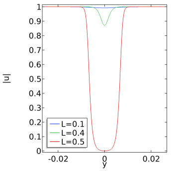
As discussed in Section 3.3, when restricting minimization of to one-dimensional competitors which in this case are functions of , we obtain full -convergence of the one-dimensional analog of to that of . Further, the behavior of minimizers of among one-dimensional competitors is determined by the value of . When exceeds a certain threshold, the bulk divergence contribution vanishes and the energy of a critical point is associated solely with a wall along the -axis that separates the regions of zero divergence. When falls below the threshold value, the bulk divergence contribution is present along with a cost of the wall associated with the jump set of the minimizer. When tends to zero, the wall disappears and the energy minimizing vector field is essentially a linear interpolation of the boundary data.
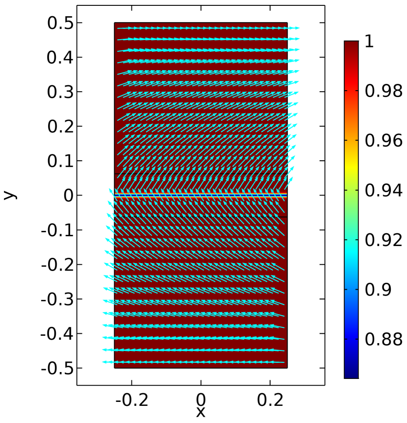
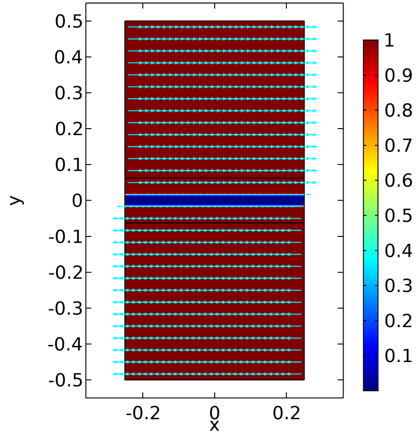
Figs. 2-3 present the results of simulations for the gradient flow for in the rectangle. It is evident that, even though the simulations are fully two-dimensional, the critical points obtained in this way are one-dimensional and conform to the picture described in the previous paragraph. Two main observations follow from these figures. First, the results seem to indicate that the wall cost is indeed one-dimensional as we conjectured earlier in the paper. Second, in all simulations done in the rectangle, the critical points we observe are always one-dimensional, even for large values of . This is in contrast to the results in [17] for the version of the problem with the Ginzburg-Landau instead of the Chern-Simons-Higgs potential. In that work, one-dimensional critical points are found to be unstable with respect to formation of cross-tie configurations for large —such instability does not seem to be present here, at least numerically.
4.2 Degrees other than or are too costly
Before we begin the constructions and numerics pertaining to , we first present a theorem which will elucidate the behavior of certain critical points for and provide an explanation for some of the morphology to come. The theorem yields a lower bound for the -norm of the divergence, in the spirit of analogous lower bound results of Jerrard [19] and Sandier [36] for the Ginzburg-Landau energy. The proofs of the Jerrard/Sandier results rely crucially on the fact that the square of the gradient of a function is a sum of squares of its components, a feature that is not shared by the square of the divergence of a vector field. We overcome this difficulty by working in Fourier space.
Theorem 4.1.
Fix , set and let be a circle of radius centered at the origin. Suppose that is such that on and for any . Then
| (4.4) | ||||
| (4.5) |
Remark 4.2.
Proof.
The proof of this result proceeds using Fourier series.
1. Developing in a Fourier series, given by
we first derive a formula for the degree of in terms of its Fourier coefficients. Denoting by the restriction of to and writing we compute
| (4.6) | ||||
| (4.7) |
where in the last line we have used orthogonality.
2. As in the proof of Thm. 5.1 in [17], we find
in where we have
It follows that
We estimate the integrals and separately as follows, beginning with From Eqn. (4.6) and the assumption that for each , we obtain that for each
| (4.8) |
Using now the definition of and the fact that we find that It follows that
| (4.9) |
We next turn to estimating Let us first suppose We have
| (4.10) | ||||
| (4.11) | ||||
| (4.12) | ||||
| (4.13) |
In going from (4.10) to (4.11) we have used (4.13) while in going from (4.11) to (4.12) we have used that This completes the proof of the theorem when so we turn our attention to when In this case, we have
∎
It also is worth mentioning that among degree 1 singularities, the -norm of the divergence can vary greatly and may or may not satisfy a lower bound of the type in the previous theorem. For example, for a Ginzburg-Landau vortex , the -norm of the divergence taken over an annulus centered at the origin blows up logarithmically as the inner radius approaches 0. However, an vortex, given by , is divergence free. This observation is relevant to our model, especially at corner-type defects on the phase boundary. In many of our examples, the director , which must be tangent to the phase boundary, switches the sense of tangency at a corner. If such a switch occurs at a corner of the phase boundary in the interior of the domain, then walls must intersect the defect in order to avoid infinite energy from the bulk divergence term; see Fig. 4. Conversely, if does not change its sense of tangency at a corner on the interface, then the singularity can be locally resolved by the formation of a partial vortex in which an infinite family of characteristics emanate from the defect.


4.3 Critical points of and in a disk.
In this section we consider critical points of the energy in the disk of radius among competitors satisfying the boundary condition
| (4.14) |
where , , and the boundary is parametrized with respect to arc-length.
The simplest cases to consider are and when for which minimizers of are the divergence-free vortex
and the constant state
respectively. Indeed, trivially, in both cases . Hence our principal interest in this section will be to understand the behavior of critical points for other choices of .
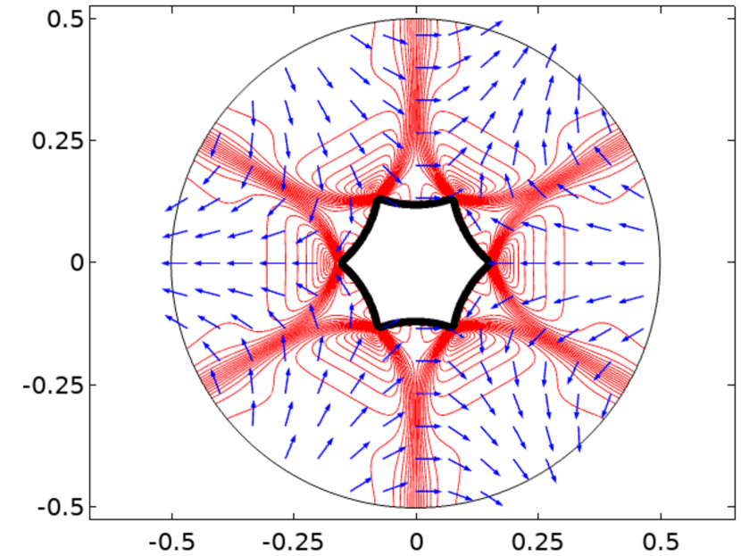
We begin by considering the case where is a negative integer and . To gain some insight into how these boundary conditions influence the morphology of interfaces and walls, we present in Figure 5 the large-time asymptotics for gradient flow dynamics for the energy with boundary conditions for two values of . Then in Figure 6 we present simulations for data with degrees and . Although we do not impose an area constraint in these simulations in order to induce a phase transition, these numerics nonetheless indicate a substantial presence of the isotropic phase in the form of an island with boundary singularities. Generally speaking, these islands appear to grow in size as grows, and for , both configurations with a single or multiple vortices are possible. Studies on vortices using the Ginzburg-Landau potential such as [8] or—more appropriately to this study—the Chern-Simons-Higgs potential with in the elastic energy [23] tempt one to think of these islands for as “defects” arising from the negative degree boundary condition. However, the numerics and Theorem 4.1 indicate that the cores of the defects do not shrink in the limit. Indeed, from Theorem 4.1 it follows that a defect with a negative degree must either be inside an isotropic region or have walls originating from the defect. The latter situation was, in fact, observed in [17] for the degree defects while the Ginzburg-Landau potential considered in [17] did not allow for presence of interfaces.
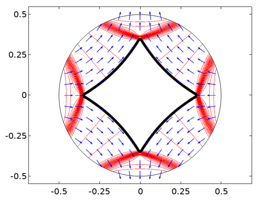
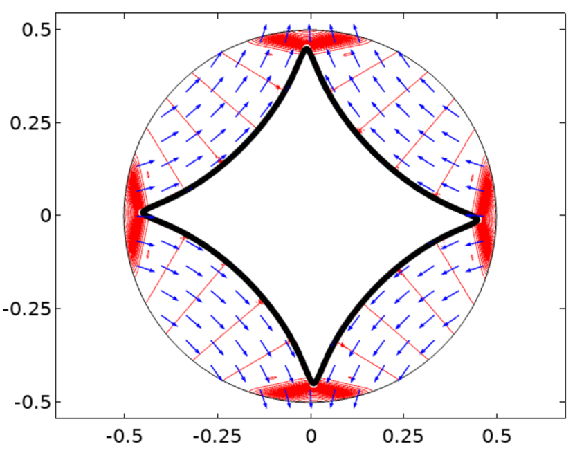
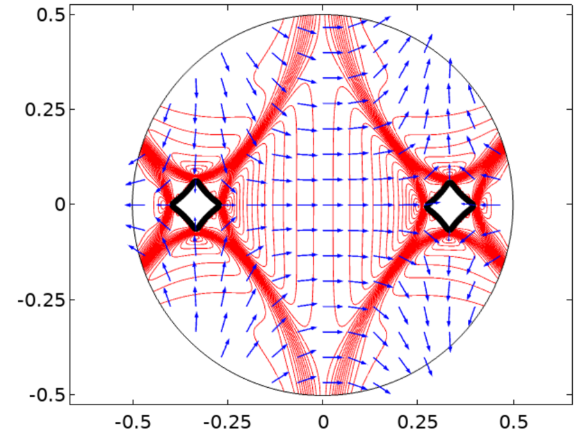
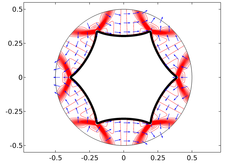
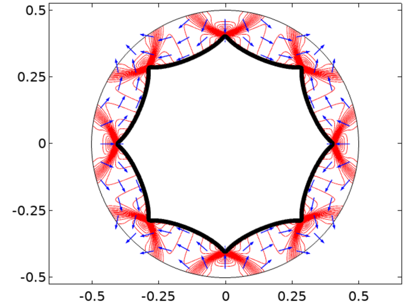
We now provide some analytical evidence that supports the observations in Figs. 5-6. Motivated by the gradient flow simulations, we construct critical points for and so divergence-free competitors for . These constructions will have only interface, but no walls, with singular points of the interface always touching the boundary of the disk, though of course the numerics suggest that for finite, there should exist walls branching off the phase boundary singularities and attaching to .
Example 4.3.
In this example, , and we are interested in competitors which exhibit the symmetry
| (4.15) |
This is the symmetry exhibited by the configurations in Figs. 5-6. The construction will proceed by issuing characteristics off and by adhering to the condition (4.3).
Owing to the condition (4.15), we construct a critical point of in the sector corresponding to and then extend the construction to the rest of the domain by symmetry. Shifting out of complex notation and parametrizing by for , we will insist that rather than just having agreement between the normal component of and that of the data.
Integrating the characteristic equations then yields
| (4.16) | ||||
| (4.17) |
with , We represent the interface in the form
for an appropriate arrival time . Here, for each , a characteristic arrives at the interface at the time and we require that at the point of arrival is tangent to the interface, that is
Using this expression in (4.16), we find that
Upon rearrangement, we have
Multiplying these equations by and , respectively, and adding the results gives
Integration then yields
Motivated by numerics, we seek an interface that meets at so that Then , so that The parametric equation of the interface in the sector is now given by
| (4.18) | ||||
| (4.19) |
Extending the interface to all of via the symmetry condition (4.15), we obtain a closed curve with evenly-spaced cusps. When one checks that and and the interface satisfies the equation In Fig. 7 we compare the graph of this curve with the contour line for the critical point obtained numerically via gradient flow when . It is clear that the two curves are very close to each other, which is quite striking since one might only expect a strong connection between the critical points of and for large.
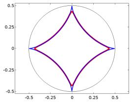
One can also check that for the construction obtained above, the area of the isotropic island increases with . In fact, a calculation that we omit goes to show that in the limit, the isotropic region fills the entire disk!
The preceding calculation can also be used in the case of in order to reconstruct parts of critical points of . Recall that, in this case, by Corollary 3.11, the characteristics are circular arcs of finite radii that may run directly from the interface to . In Fig. 5, for example, red curves correspond to level sets of and thus the characteristics for connect large portions of the interface to the boundary. In order to fully reproduce the critical point of completely, however, one needs to allow for the presence of walls, as evidenced by the gradient flow numerics in Fig. 5. Although a similar approach yielded critical points of (1.3) for degree boundary data in [17], such a construction will be more elaborate here and we do not pursue this issue further in the present paper.
We conclude this section by considering the boundary data in (4.14) corresponding to positive and . The results of the gradient flow simulations are shown in Fig. 8. Not surprisingly, when is small for , the stable configuration consists of two degree one vortices looking locally like , see Fig. 8(a). As increases, however, these vortices collapse onto and spread along while forming two walls along the upper and lower halves of the boundary, respectively, cf. Fig. 8(b). Indeed this simulation suggests that for with large, the preferred state is . In fact, if one tries to construct a competitor having a ‘boundary wall’ for this boundary data, that is, a unit vector field such that the normal component of the data is met but the tangential component switches sign, then one finds
and
Thus such a competitor must have trace along and there is no need then to accumulate divergence inside the disk by varying from constancy.
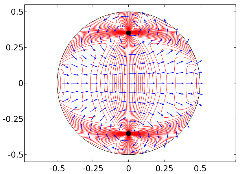
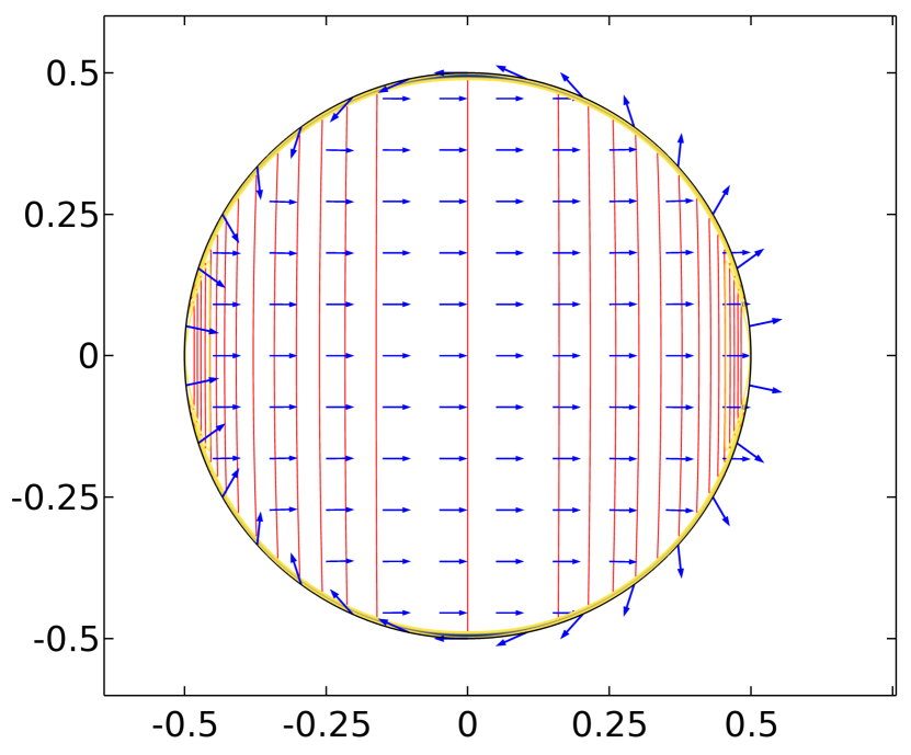
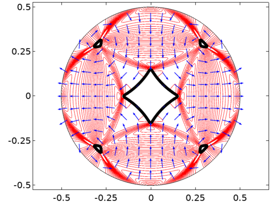
In the case of a degree boundary data, cf. Figure 8(c), the behavior is more complex—the degree vortex appears to split into four degree vortices and one degree vortex. The four vortices approach the boundary of the domain with an increasing while the degree vortex remains at the center of the disk.
We use the simulations in the case of to test Conjecture (3.12) on the one-dimensional character of the wall cost. The walls in this example turn out to be significantly deeper than in other cases that we considered and it is therefore easier to compare the numerically computed wall profiles with the corresponding heteroclinic connection. Consider the critical point for depicted in Fig. 8(b). For a large value of the defects present inside for small spread along the boundary to form two boundary walls. Due to symmetry, it is sufficient to consider the wall in the first quadrant. Then along each ray emanating at angle from the origin, the wall connects the vector to the vector . Because the normal to the boundary/interface is , the normal component of the vector field is continuous across the wall, while the tangential component reverses sign. The jump in the tangential component across the wall grows as changes from to . In Fig. 9(a) we plot cross-sections of for the critical point of shown in Fig. 8(b), where the cross-sections are shown along several rays . In Fig. 9(b),
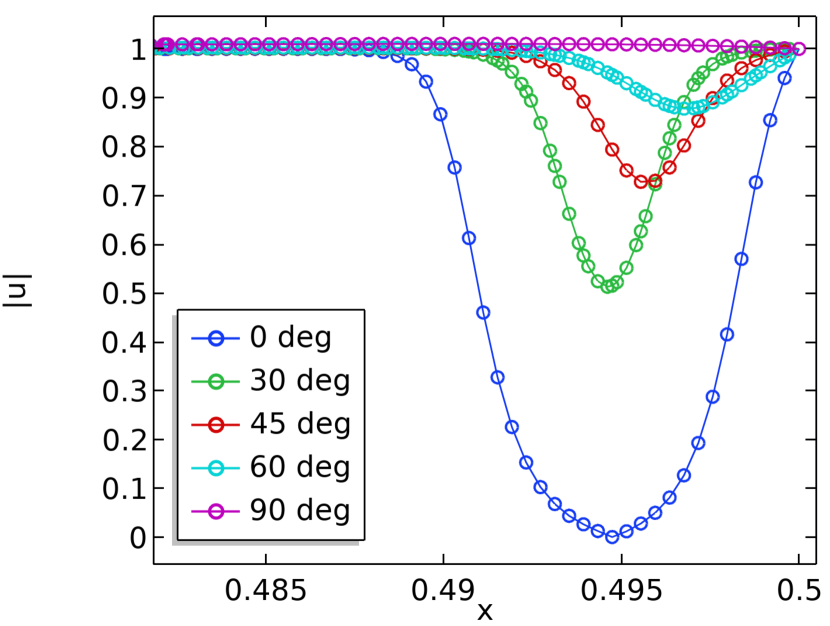
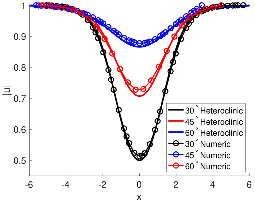
the same scaled and translated profiles are shown together with the corresponding solutions of the ODE that describes a heteroclinic connection associated with , assuming one-dimensional cost. As Fig. 9(b) demonstrates, the graphs are close to each other for all respective values of —this is in agreement with our conjecture that the cost is one-dimensional.
4.4 Examples for Degree Zero Boundary Data
In this section, we analytically and numerically construct an example with an isotropic tactoid which exhibits two defects on the phase boundary. Let us describe a key feature of this example. Recall that at a nematic-isotropic interface for , the trace of a competitor from the nematic region is tangent to the interface, cf. (3.4). If, for example, is smooth and does not change the sense of tangency along the interface, then the degree of around any connected component of the interface is . If we specify a degree boundary condition around or at infinity, this mismatch can be rectified by the presence of two defects along the interface, similar to the construction of the recovery sequence in Section 2. This is the effect we will see in the following example.
We begin with some numerics. Fig. 12(a) shows the result of gradient flow simulation in a large rectangular domain with constant boundary data . We observe in Fig. 12(a) that (i) the interface surrounds a single isotropic island, (ii) there appear to be two walls which intersect the two defects on the interface, and (iii) the solutions possess the symmetries
and
Furthermore, in Fig. 12(a) we see that (iv) the walls divide the plane into three regions, with
| (4.20) |
This simulation, though depicting transient behavior, leads us to seek a critical point of satisying (i)-(iv) consisting of an isotropic tactoid in an infinite sea of nematic, where in the far field, . To induce a static–and presumably stable–critical point having an isotropic phase, we will enforce an area constraint of the form
The complication here–and it is a significant one–is that an interface and a wall are rigidly linked via the straight-line characteristics lying in between them, and the requirement of tangency of along the interface and agreement of the normal component of with that of along the wall make the construction rather daunting.
Somewhat surprisingly, we are able to achieve this construction by deriving a formula of the form
| (4.21) |
for an explicit , for competitors satisfying (i)–(iv), where is the angle the tangent vector to makes with the horizontal. For such , the energy therefore only depends on the interface, a reflection of the afore-mentioned rigidity of this problem. We then consider variations of the interface to derive an ODE (4.45) for along with the junction condition (4.46) at the intersection of walls and interfaces. Numerically integrating this ODE yields a configuration which closely resembles the results of the simulations shown in Figure 12(a), cf. Figure 12(b). The Role of Walls: Before embarking on this construction, let us comment on the role of walls in this example. A natural question is: given these conditions, namely an area constraint on the isotropic region and the requirement that in the far field, is it necessary for a critical point to have walls? While we do not as yet have a proof, we believe the answer is yes. Let us present some heuristic arguments to this effect. Working within the symmetry assumption (iii), consider the possibility of constructing a competitor without walls. Then one of the two configurations depicted in Fig. 10 are possible where the isotropic island either has two corners and no walls or it has two cusps and no walls. In the former case, one can show that partial vortices should form near the corners in the nematic phase, causing the divergence contribution to the energy to blow up; see Fig. 4 above. If there are two cusps and no walls, Fig. 10 demonstrates that this is not possible as the characteristics emanating from the interface would have to intersect non-tangentially. In light of these observations, junctions between interfaces and walls appear to be fairly generic, making in particular the junction condition (3.80) potentially important when analyzing candidates for possible critical points or minimizers when is finite.
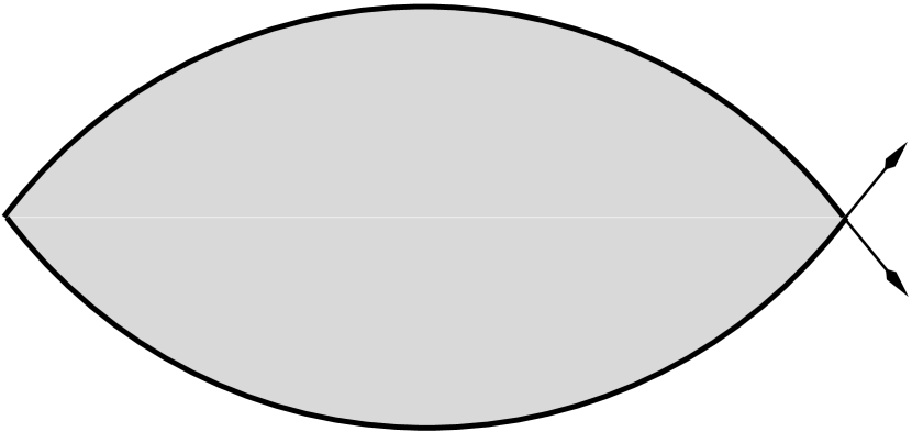
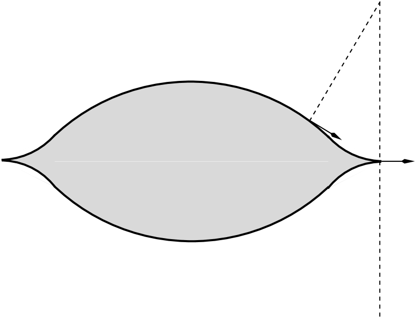
Example 4.4.
For this calculation, by (iii), it suffices to consider the problem in the first quadrant . Let us assume that is smooth and can be parametrized by where , with on the -axis and on the -axis; see Figure 11.
We do not assume that the interface is parametrized by the arclength variable in this derivation. Then
| (4.22) |
Let us define
and the normal vector
We now deduce the location of the wall, which we will see is determined by the interface. Recall that in light of (4.3), is perpendicular to the straight characteristics, which themselves intersect the interface perpendicularly, so we can parametrize the wall by shooting characteristics off of the interface until they hit the wall. We can write a parametrized path for the wall then as
| (4.23) |
Hence by (4.22) the trace of on the wall from the left, denoted here by , is given by
| (4.24) |
We define a function by the equation
Then the tangent and normal vectors to the wall are given by
| (4.25) |
Next, we collect some relations between several of the above quantities which will be useful in the following calculations. From the continuity of the normal traces across a wall, we have
which we rewrite using (4.24), (4.25), and the angle subtraction identity for as
| (4.26) |
Similarly, the condition for the tangential components across a wall, cf. (3.4), can be expressed as
| (4.27) |
From (4.26), (4.27) it follows that for some integer , and is in fact since at , . Thus
| (4.28) |
We can now write the energy in the first quadrant as
| (4.29) |
One can use (4.23) and the orthogonality of and to easily calculate
Substituting this and
into (4.29) yields
| (4.30) |
In order to obtain a formula for depending only on the interface, it remains to simplify
| (4.31) |
We begin this simplification by finding an expression for in terms of and . Using the definitions (4.22), (4.23), and (4.25) for , , and , respectively, along with (4.28), we calculate
| (4.32) |
Expanding out (4.32) and using the angle subtraction formulae for sine and cosine eventually gives
| (4.33) |
Now we observe from our symmetry assumption on that on the -axis, so that . If we assume that does not reach until , which in terms of the interface means that
| (4.34) |
then we can divide (4.33) by . This results in the following ODE for :
| (4.35) |
Multiplying both sides of (4.35) by the integrating factor
results in
Integrating both sides, dividing by , and using the half angle formula for cosine, we obtain
| (4.36) |
Finally, let us record the identity
| (4.37) |
which follows from rearranging (4.33).
We now use the formula (4.36) for to calculate (4.31), the quantity we set out to simplify. Let us assume that , which means that
| (4.38) |
Then plugging in (4.37) for (4.31) and using the assumptions (4.34) and (4.38), namely and , we write
Utilizing the formula (4.36) to calculate and then a half angle formula for cosine and a double angle formula for sine, we arrive at
| (4.39) |
Now we are ready to use the expression (4.39) for (4.31) in the energy (4.30). We have
We focus on the term
| (4.40) |
Let us define the function by the equations
It follows from (3.8) that remains finite as approaches so long as approaches as at least as fast as for some and , an assumption which is satisfied by . A straightforward calculation, which we omit, using the chain rule, the definition of , and some trigonometric identities yields
| (4.41) |
Inserting this expression into the last integral in (4.40), that term becomes
| (4.42) |
which we integrate by parts to obtain
Note that by our symmetry assumptions, , so that
| (4.43) |
We combine (4.41)–(4.43) to rewrite (4.40):
| (4.44) |
Using the right hand side of (4.44) for (4.40), we finally have
Thus we arrive at (4.21).
We turn now to the criticality conditions for . For any with smooth interface, we parametrize the interface of length by arclength . Then the standard derivation [4] gives the following condition on the interface
| (4.45) |
along with the the junction condition
| (4.46) |
at , the intersection of with the -axis.
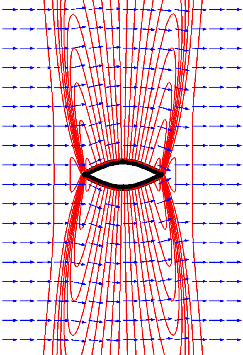
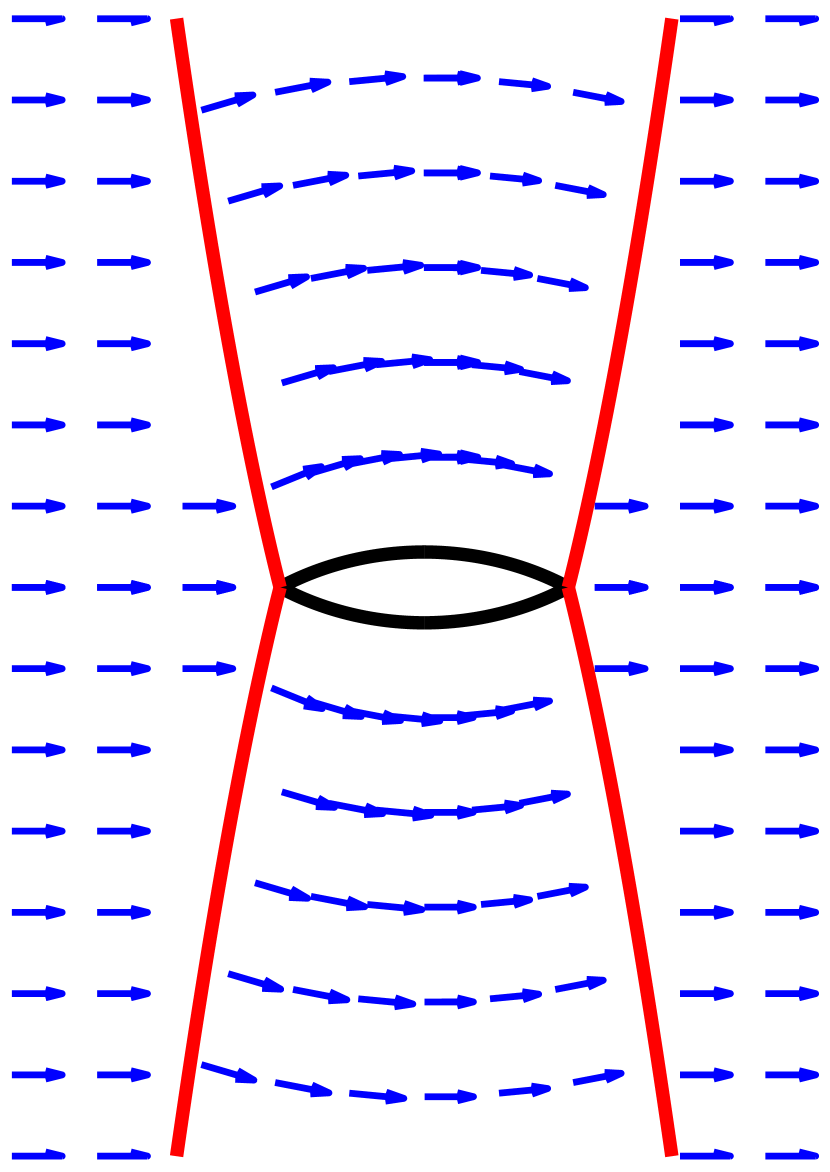
5 Appendix
We present here the proof of Theorem 3.13. See Fig. LABEL:Junctionfig for a guide to the notation.
Proof.
The derivation of (5.19) follows the same general lines as those appearing in the proof of Theorem 3.12. However, a major complicating consideration is that it is no longer possible to assume that the deforming vector field is normal to all four curves since they all meet at . Instead we will have to incorporate tangential components of along these four curves as well.
To this end, we assume simply that and again introduce the map via (3.63). We assume that each is smoothly parametrized by arclength through a map for some with . Then we replace (3.62) by
| (5.1) |
where
As a consequence of the compact support of , we have that
| (5.2) |
but we stress that none of these functions is assumed to vanish at , namely at the location of the junction .
We now deform each region , for by the map to form four contiguous regions and we deform the four boundary curves to form four new boundary curves Of course the junction point is also carried along by this flow.
The four curves are parametrized by which we denote by though no longer represents arclength. Indeed one calculates that
| (5.3) |
from which it follows that
| (5.4) |
where denotes the curvature of at (compare with (3.68)) and we have invoked the Frenet relations and . A related calculation goes to show that the unit normal to is given by
| (5.5) |
Now in the ball the unperturbed critical point is given by
and we wish to perturb it into a new function given by
To carry this out, as in the previous proof, we extend the domain of definition of to a neighborhood of in such a way that the extension is constant along the normals to the boundary of its original domain of definition. Then we introduce three functions and such that
| (5.6) |
so as to preserve the required -valued nature of
We must also take care to preserve the property in the sense of (3.45) and this requires that the following four conditions hold to along and respectively:
| (5.7) |
We note that the first and last of these conditions implies at that either or along and likewise either or along .
Substituting (5.3) and (5.5) into the four conditions of (5.7), and expanding to , a tedious but straight-forward calculation leads to the following requirements relating the traces of the to :
| (5.8) | |||
| (5.9) | |||
| (5.10) | |||
| (5.11) |
for
With the perturbations of the four curves and three functions defined, we are ready to compute the variation of in a neighborhood of the junction point . Carrying out the calculation (3.77) in for and then applying the divergence theorem we find with the aid of (3.46) that
where we have used the fact that , , etc.
Now we appeal to the relations (5.8)–(5.11), along with the conditions and and perform an integration by parts to find
| (5.12) |
We turn now to calculating the variations of the four jump energies. We begin by invoking (5.4) to compute
Thus,
| (5.13) |
To compute the variation in the jump energies over and requires an expansion to of the quantities and Substituting the expression for from (5.3) into the formula for from (5.6) and Taylor expanding in we find with the use of (5.5) that along we have
| (5.14) | |||
| (5.15) |
where and in the expression above are evaluated at and In the last line we have also used that our extension of was constant along to eliminate the term that would other have been present upon Taylor expanding.
Similarly, we calculate that along we have
| (5.16) |
Now since
and
we have that
and
Using these last two identities in (5) and integrating by parts implies that
| (5.17) |
Then invoking the criticality condition (3.47) from Theorem 3.9 and integrating by parts we can rewrite this identity as
| (5.18) |
Now we can combine (5.12), (5.13) and (5.18), and through a use of the criticality conditions (3.60) and (3.61) of Theorem 3.12 we find that all integrals over the four curves drop, leaving only
Recall now that , , etc. Thus, the arbitrary value of the vector , implies that a vanishing first variation leads to the necessary condition at a junction of the form
| (5.19) |
where all quantities above are evaluated at the junction .
∎
Acknowledgments. PS, MR and RV acknowledge the support from NSF DMS-1362879 and a Simons Collaboration grant 585520. RV also acknowledges the support from an Indiana University College of Arts and Sciences Dissertation Year Fellowship. The research of RV was also partially supported by the Center for Nonlinear Analysis at Carnegie Mellon University and by NSF DMS-1411646. DG acknowledges the support from NSF DMS-1729538.
References
- [1] COMSOL Multiphysics® v. 5.3. http://www.comsol.com/. COMSOL AB, Stockholm, Sweden.
- [2] Alouges, F., Rivière, T., and Serfaty, S. Néel and cross-tie wall energies for planar micromagnetic configurations. ESAIM Control Optim. Calc. Var. 8 (2002), 31–68. A tribute to J. L. Lions.
- [3] Ambrosio, L., De Lellis, C., and Mantegazza, C. Line energies for gradient vector fields in the plane. Calc. Var. Partial Differential Equations 9, 4 (1999), 327–255.
- [4] Angenent, S., and Gurtin, M. E. Multiphase thermomechanics with interfacial structure 2. Evolution of an isothermal interface. Arch. Ration. Mech. Anal. 108, 3 (Nov 1989), 323–391.
- [5] Aviles, P., and Giga, Y. On lower semicontinuity of a defect energy obtained by a singular limit of the Ginzburg-Landau type energy for gradient fields. Proc. Roy. Soc. Edinburgh Sect. A 129, 1 (1999), 1–17.
- [6] Baldo, S. Minimal interface criterion for phase transitions in mixtures of Cahn-Hilliard fluids. Ann. Inst. H. Poincaré Anal. Non Linéaire 7, 2 (1990), 67–90.
- [7] Bauman, P., Park, J., and Phillips, D. Analysis of nematic liquid crystals with disclination lines. Arch. Ration. Mech. Anal. 205, 3 (2012), 795–826.
- [8] Bethuel, F., Brezis, H., and Hélein, F. Ginzburg-Landau vortices, vol. 13 of Progress in Nonlinear Differential Equations and their Applications. Birkhäuser Boston, Inc., Boston, MA, 1994.
- [9] Conti, S., and De Lellis, C. Sharp upper bounds for a variational problem with singular perturbation. Math. Ann. 338, 1 (2007), 119–146.
- [10] De Lellis, C., and Otto, F. Structure of entropy solutions to the eikonal equation. J. Eur. Math. Soc. (JEMS) 5, 2 (2003), 107–145.
- [11] DeBenedictis, A., and Atherton, T. J. Shape minimisation problems in liquid crystals. Liquid Crystals 43, 13-15 (2016), 2352–2362.
- [12] DeSimone, A., Kohn, R. V., Müller, S., and Otto, F. A compactness result in the gradient theory of phase transitions. Proc. Roy. Soc. Edinburgh Sect. A 131, 4 (2001), 833–844.
- [13] Fang, J., Teer, E., Knobler, C. M., Loh, K.-K., and Rudnick, J. Boojums and the shapes of domains in monolayer films. Phys. Rev. E 56 (Aug 1997), 1859–1868.
- [14] Fonseca, I. The wulff theorem revisited. Proceedings: Mathematical and Physical Sciences 432, 1884 (1991), 125–145.
- [15] Fonseca, I., and Müller, S. Quasi-convex integrands and lower semicontinuity in . SIAM J. Math. Anal. 23, 5 (1992), 1081–1098.
- [16] Giusti, E. Minimal surfaces and functions of bounded variation, vol. 80 of Monographs in Mathematics. Birkhäuser Verlag, Basel, 1984.
- [17] Golovaty, D., Sternberg, P., and Venkatraman, R. A Ginzburg-Landau type problem for highly anisotropic nematic liquid crystals. To appear in SIAM J. Math. Anal. (2018).
- [18] Ignat, R. Singularities of divergence-free vector fields with values into or . Applications to micromagnetics. Confluentes Math. 4, 3 (2012), 1230001, 80.
- [19] Jerrard, R. L. Lower bounds for generalized Ginzburg-Landau functionals. SIAM J. Math. Anal. 30, 4 (1999), 721–746.
- [20] Jin, W., and Kohn, R. V. Singular perturbation and the energy of folds. J. Nonlinear Sci. 10, 3 (2000), 355–390.
- [21] Kim, Y.-K., Shiyanovskii, S. V., and Lavrentovich, O. D. Morphogenesis of defects and tactoids during isotropic–nematic phase transition in self-assembled lyotropic chromonic liquid crystals. Journal of Physics: Condensed Matter 25, 40 (2013), 404202.
- [22] Kohn, R. V., and Sternberg, P. Local minimisers and singular perturbations. Proc. Roy. Soc. Edinburgh Sect. A 111, 1-2 (1989), 69–84.
- [23] Kurzke, M., and Spirn, D. Gamma limit of the nonself-dual Chern-Simons-Higgs energy. J. Funct. Anal. 255, 3 (2008), 535–588.
- [24] Lamy, X., and Otto, F. On the regularity of weak solutions to Burgers’ equation with finite entropy production. Calc. Var. PDE 57, 4 (2018), Art. 94, 19.
- [25] Lorent, A. A simple proof of the characterization of functions of low Aviles Giga energy on a ball via regularity. ESAIM Control Optim. Calc. Var. 18, 2 (2012), 383–400.
- [26] Lorent, A. A quantitative characterisation of functions of low Aviles Giga energy in convex domains. Ann. Sc. Norm. Super. Pisa Cl. Sci. (5) 13, 1 (2014), 1–66.
- [27] Modica, L. The gradient theory of phase transitions and the minimal interface criterion. Arch. Ration. Mech. Anal. 98, 2 (1987), 123–142.
- [28] Mottram, N. J., and Newton, C. J. Introduction to Q-tensor theory. arXiv preprint arXiv:1409.3542 (2014).
- [29] Murat, F. Compacité par compensation. Ann. Scuola Norm. Sup. Pisa Cl. Sci. (4) 5, 3 (1978), 489–507.
- [30] Murat, F. L’injection du cône positif de dans est compacte pour tout . J. Math. Pures Appl. (9) 60, 3 (1981), 309–322.
- [31] Novack, M. R. Dimension reduction for the Landau-de Gennes model: the vanishing nematic correlation length limit. To appear in SIAM J. Math. Anal. (2018).
- [32] Owen, N. C., Rubinstein, J., and Sternberg, P. Minimizers and gradient flows for singularly perturbed bi-stable potentials with a Dirichlet condition. Proc. Roy. Soc. London Ser. A 429, 1877 (1990), 505–532.
- [33] Poliakovsky, A. On the -limit of singular perturbation problems with optimal profiles which are not one-dimensional. Part I: The upper bound. Differential Integral Equations 26, 9-10 (2013), 1179–1234.
- [34] Poliakovsky, A. On the -limit of singular perturbation problems with optimal profiles which are not one-dimensional. Part II: The lower bound. Israel J. Math. 210, 1 (2015), 359–398.
- [35] Rudnick, J., and Bruinsma, R. Shape of domains in two-dimensional systems: Virtual singularities and a generalized wulff construction. Phys. Rev. Lett. 74 (Mar 1995), 2491–2494.
- [36] Sandier, E. Lower bounds for the energy of unit vector fields and applications. J. Funct. Anal. 152, 2 (1998), 379–403.
- [37] Sternberg, P. The effect of a singular perturbation on nonconvex variational problems. Arch. Ration. Mech. Anal. 101, 3 (1988), 209–260.
- [38] Tartar, L. Compensated compactness and applications to partial differential equations. In Nonlinear analysis and mechanics: Heriot-Watt Symposium, Vol. IV, vol. 39 of Res. Notes in Math. Pitman, Boston, Mass.-London, 1979, pp. 136–212.
- [39] van Bijnen, R. M. W., Otten, R. H. J., and van der Schoot, P. Texture and shape of two-dimensional domains of nematic liquid crystals. Phys. Rev. E 86 (Nov 2012), 051703.