Inverse obstacle scattering problem for elastic waves with phased or phaseless far-field data

Abstract.

This paper concerns an inverse elastic scattering problem which is to determine the location and the shape of a rigid obstacle from the phased or phaseless far-field data for a single incident plane wave. By introducing the Helmholtz decomposition, the model problem is reduced to a coupled boundary value problem of the Helmholtz equations. The relation is established between the compressional or shear far-field pattern for the elastic wave equation and the corresponding far-field pattern for the coupled Helmholtz equations. An efficient and accurate Nyström type discretization for the boundary integral equation is developed to solve the coupled system. The translation invariance of the phaseless compressional and shear far-field patterns are proved. A system of nonlinear integral equations is proposed and two iterative reconstruction methods are developed for the inverse problem. In particular, for the phaseless data, a reference ball technique is introduced to the scattering system in order to break the translation invariance. Numerical experiments are presented to demonstrate the effectiveness and robustness of the proposed method.

1. Introduction

Scattering problems for elastic waves have significant applications in seismology and geophysics [27]. As an important research topic in scattering theory, the inverse obstacle scattering problem (IOSP) is to identify unknown objects that is not accessible by direct observation through the use of waves. The IOSP for elastic waves have continuously attracted much attention by many researchers. The recent development can be found in [1] on mathematical and numerical methods for solving the IOSP in elasticity imaging.

The phased IOSP refers to as the IOSP by using full scattering data which contains both phase and amplitude information. The phased IOSP for elastic waves has been extensively studied and a great deal of mathematical and numerical results are available. In [28, 29, 33], the domain derivatives were investigated by using either the boundary integral equation method or the variational method. In [39], based on the Helmholtz decomposition, the boundary value problem of the Navier equation was converted into a coupled boundary value problem of the Helmholtz equations. A frequency continuation method was developed to reconstruct the shape of the obstacles. We refer to [11, 9] for the uniqueness results on the inverse elastic obstacle scattering problem. Related work can be found in [26, 5, 12, 17, 22, 37, 13, 34] on the general inverse scattering problems for elastic waves.

In many practical applications, the phase of a signal either can be very difficult to be measured or can not be measured accurately compared with its amplitude or intensity. Thus it is often desirable to solve the problems with phaseless data, which are called phase retrieval problems in optics, or physical and engineering sciences. Due to the translation invariance property of the phaseless wave field, it is impossible to reconstruct uniquely the location of the unknown objects, which makes the phaseless inverse scattering problems much more difficult compared to the phased case. Various numerical methods have been proposed to solve the phaseless IOSP for acoustic waves governed by the scalar Helmholtz equation. In [25], Kress and Rundell proposed a Newton’s iterative method for imaging a two-dimensional sound-soft obstacle from the phaseless far-field data with one incident wave. A nonlinear integral equation method was developed in [14, 15] for the two- and three-dimensional shape reconstruction from a given incident field and the modulus of the far-field data, respectively. The nonlinear integral equation method proposed by Johansson and Sleeman [16] was extended to reconstruct the shape of a sound-soft crack by using phaseless far-field data for one incident plane wave in [10]. In addition, fundamental solution method [18] and a hybrid method [30] were proposed to detect the shape of a sound-soft obstacle by using of the modulus of the far-field data for one incident field. To overcome the nonuniqueness issue, Zhang et al. [42, 43] proposed to use superposition of two plane waves with different incident directions as the illuminating field to recover both of the location and the shape of an obstacle simultaneously by using phaseless far-field data. Recently, a reference ball technique was developed in [8] to break the translation invariance and reconstruct both the location and shape of an obstacle from phaseless far-field data for one incident plane wave. We refer to [38, 35, 40] for the uniqueness results on the inverse scattering problems by using phaseless data. For related phaseless inverse scattering problems as well as numerical methods may be found in [2, 31, 6, 4, 3, 36, 41, 19, 20].

In this paper, we consider the inverse elastic scattering problem of determining the location and shape of a rigid obstacle from phased or phaseless far-field data for a single incident plane wave. Motivated by the recent work in [8, 10], the reference ball technique in [32, 40], and the Helmholtz decomposition in [39], we propose a nonlinear integral equation method combined with the reference ball technique to solve the IOSP for elastic waves. In particular, for the phaseless IOSP, since the location of the reference ball is known, the method has the capability of calibrating the scattering system so that the translation invariance does not hold anymore. Therefore, the location information of the obstacle can be recovered with negligible additional computational costs. Moreover, we develop a Nyström type discretization for the integral equation to efficiently and accurately solve the direct obstacle scattering problem for elastic waves. It is worth mentioning that the proposed method for phased and phaseless IOSP are extremely efficient since we only need to solve the scalar Helmholtz equations and avoid solving the vector Navier equations. The goal of this work is fivefold: establish the relationship between the compressional or shear far-field pattern for the Navier equation and the corresponding far-field pattern for the coupled Helmholtz system; prove the translation invariance property of the phaseless compressional and shear far-field pattern; develop a Nyström discretization for the boundary integral equation to solve the direct obstacle scattering problems for elastic waves; propose a nonlinear integral equation method to reconstruct the obstacle’s location and shape by using far-field data for one incident plane wave; develop a reference ball based nonlinear integral equation method to reconstruct the obstacle’s location and shape by using phaseless far-field data for one incident plane wave.

The paper is organized as follows. In Section 2, we introduce the problem formulation. Section 3 establishes the relationship of the far-field patterns between the elastic wave equation and the coupled Helmholtz system. In Section 4, a Nyström-type discretization is developed to solve the coupled boundary value problem of the Helmholtz equations. In Section 5, a nonlinear integral equation method and a reference ball based iterative method are present to solve the phased and phaseless IOSP, respectively. Numerical experiments are shown to demonstrate the feasibility of the proposed methods in Section 6. The paper is concluded with some general remarks and directions for future work in Section 7.

2. Problem formulation

Consider a two-dimensional elastically rigid obstacle, which is described as a bounded domain $D\subset\mathbb{R}^{2}$ with $\mathcal{C}^{2}$ boundary $\Gamma_{D}$. Denote by $\nu=(\nu_{1},\nu_{2})^{\top}$ and $\tau=(\tau_{1},\tau_{2})^{\top}$ the unit normal and tangential vectors on $\Gamma_{D}$, respectively, where $\tau_{1}=-\nu_{2},\tau_{2}=\nu_{1}$. The exterior domain $\mathbb{R}^{2}\setminus\overline{D}$ is assumed to be filled with a homogeneous and isotropic elastic medium with a unit mass density.

Let the obstacle be illuminated by a time-harmonic plane wave $\boldsymbol{u}^{\rm inc}$, which satisfies the two-dimensional Navier equation:

$$\mu\Delta\boldsymbol{u}^{\rm inc}+(\lambda+\mu)\nabla\nabla\cdot\boldsymbol{u}^{\rm inc}+\omega^{2}\boldsymbol{u}^{\rm inc}=0\quad{\rm in}~{}\mathbb{R}^{2}\setminus\overline{D},$$

where $\omega>0$ is the angular frequency and $\lambda,\mu$ are the Lamé constants satisfying $\mu>0,\lambda+\mu>0$. Explicitly, we have

$$\boldsymbol{u}^{\rm inc}(x)=d\mathrm{e}^{{\rm i}\kappa_{\rm p}d\cdot x}\quad\text{or}\quad\boldsymbol{u}^{\rm inc}(x)=d^{\perp}\mathrm{e}^{{\rm i}\kappa_{\rm s}d\cdot x},$$

where the former is the compressional plane wave and the latter is the shear plane wave. Here $d=(\cos\theta,\sin\theta)^{\top}$ is the unit propagation direction vector, $\theta\in[0,2\pi)$ is the incident angle, $d^{\perp}=(-\sin\theta,\cos\theta)^{\top}$ is an orthonormal vector of $d$, and

$$\kappa_{\rm p}=\frac{\omega}{\sqrt{\lambda+2\mu}},\quad\kappa_{\rm s}=\frac{\omega}{\sqrt{\mu}}$$

are the compressional wavenumber and the shear wavenumber, respectively.

The displacement of the total field $\boldsymbol{u}$ also satisfies the Navier equation

$$\mu\Delta\boldsymbol{u}+(\lambda+\mu)\nabla\nabla\cdot\boldsymbol{u}+\omega^{2}\boldsymbol{u}=0\quad{\rm in}\,\mathbb{R}^{2}\setminus\overline{D}.$$

Since the obstacle is rigid, the total field $\boldsymbol{u}$ satisfies

$$\boldsymbol{u}=0\quad{\rm on}~{}\Gamma_{D}.$$

The total field $\boldsymbol{u}$ consists of the incident field $\boldsymbol{u}^{\rm inc}$ and the scattered field $\boldsymbol{v}$, i.e.,

$$\boldsymbol{u}=\boldsymbol{u}^{\rm inc}+\boldsymbol{v}.$$

It is easy to verify that the scattered field $\boldsymbol{v}$ satisfies the boundary value problem

$$\begin{cases}\mu\Delta\boldsymbol{v}+(\lambda+\mu)\nabla\nabla\cdot\boldsymbol{v}+\omega^{2}\boldsymbol{v}=0\quad&{\rm in}~{}\mathbb{R}^{2}\setminus\overline{D},\\ \boldsymbol{v}=-\boldsymbol{u}^{\rm inc}\quad&{\rm on}~{}\Gamma_{D}.\end{cases}$$ (2.1)

In addition, the scattered field $\boldsymbol{v}$ is required to satisfy the Kupradze–Sommerfeld radiation condition

$$\lim_{\rho\to\infty}\rho^{\frac{1}{2}}(\partial_{\rho}\boldsymbol{v}_{\rm p}-{\rm i}\kappa_{\rm p}\boldsymbol{v}_{\rm p})=0,\quad\lim_{\rho\to\infty}\rho^{\frac{1}{2}}(\partial_{\rho}\boldsymbol{v}_{\rm s}-{\rm i}\kappa_{\rm s}\boldsymbol{v}_{\rm s})=0,\quad\rho=|x|,$$

where

$$\boldsymbol{v}_{\rm p}=-\frac{1}{\kappa_{\rm p}^{2}}\nabla\nabla\cdot\boldsymbol{v},\quad\boldsymbol{v}_{\rm s}=\frac{1}{\kappa_{\rm s}^{2}}{\bf curl}{\rm curl}\boldsymbol{v},$$

are known as the compressional and shear wave components of $\boldsymbol{v}$, respectively. Given a vector function $\boldsymbol{v}=(v_{1},v_{2})^{\top}$ and a scalar function $v$, define the scalar and vector curl operators:

$${\rm curl}\boldsymbol{v}=\partial_{x_{1}}v_{2}-\partial_{x_{2}}v_{1},\quad{\bf curl}v=(\partial_{x_{2}}v,-\partial_{x_{1}}v)^{\top}.$$

For any solution $\boldsymbol{v}$ of the elastic wave equation (2.1), the Helmholtz decomposition reads

$$\boldsymbol{v}=\nabla\phi+\boldsymbol{\rm curl}\psi.$$ (2.2)

Combining (2.2) and (2.1), we may obtain the Helmholtz equations

$$\Delta\phi+\kappa_{\rm p}^{2}\phi=0,\quad\Delta\psi+\kappa_{\rm s}^{2}\psi=0.$$

As usual, $\phi$ and $\psi$ are required to satisfy the Sommerfeld radiation conditions

$$\lim_{\rho\to\infty}\rho^{\frac{1}{2}}(\partial_{\rho}\phi-{\rm i}\kappa_{\rm p}\phi)=0,\quad\lim_{\rho\to\infty}\rho^{\frac{1}{2}}(\partial_{\rho}\psi-{\rm i}\kappa_{\rm s}\psi)=0,\quad\rho=|x|.$$

Combining the Helmholtz decomposition and boundary condition on $\Gamma_{D}$ yields that

$$\boldsymbol{v}=\nabla\phi+{\bf curl}\psi=-\boldsymbol{u}^{\rm inc}.$$

Taking the dot product of the above equation with $\nu$ and $\tau$, respectively, we get

$$\partial_{\nu}\phi+\partial_{\tau}\psi=f_{1},\quad\partial_{\tau}\phi-\partial_{\nu}\psi=f_{2},$$

where

$$f_{1}=-\nu\cdot\boldsymbol{u}^{\rm inc},\quad f_{2}=-\tau\cdot\boldsymbol{u}^{\rm inc}.$$

In summary, the scalar potential functions $\phi,\psi$ satisfy the coupled boundary value problem

$$\begin{cases}\Delta\phi+\kappa_{\rm p}^{2}\phi=0,\quad\Delta\psi+\kappa_{\rm s}^{2}\psi=0\quad&{\rm in}~{}\mathbb{R}^{2}\setminus\overline{D},\\ \partial_{\nu}\phi+\partial_{\tau}\psi=f_{1},\quad\partial_{\tau}\phi-\partial_{\nu}\psi=f_{2}\quad&{\rm on}~{}\Gamma_{D},\\ \displaystyle{\lim_{\rho\to\infty}\rho^{\frac{1}{2}}(\partial_{\rho}\phi-{\rm i}\kappa_{\rm p}\phi)=0},\quad\displaystyle{\lim_{\rho\to\infty}\rho^{\frac{1}{2}}(\partial_{\rho}\psi-{\rm i}\kappa_{\rm s}\psi)=0},\quad&\rho=|x|.\end{cases}$$ (2.3)

It is well known that a radiating solution of (2.1) has the asymptotic behavior of the form

$$\boldsymbol{v}(x)=\frac{\mathrm{e}^{\mathrm{i}\kappa_{\rm p}|x|}}{\sqrt{|x|}}\boldsymbol{v}_{\rm p}^{\infty}(\hat{x})+\frac{\mathrm{e}^{\mathrm{i}\kappa_{\rm s}|x|}}{\sqrt{|x|}}\boldsymbol{v}_{\rm s}^{\infty}(\hat{x})+\mathcal{O}\left(\frac{1}{|x|^{\frac{3}{2}}}\right),\quad|x|\to\infty$$

uniformly in all directions $\hat{x}:=x/|x|$, where $\boldsymbol{v}_{\rm p}^{\infty}$ and $\boldsymbol{v}_{\rm s}^{\infty}$, defined on the unit circle $\Omega$, are known as the compressional and shear far-field pattern of $\boldsymbol{v}$, respectively. Define $(a_{\rm p},a_{\rm s}):=(1,0)$ or $(0,1)$, where $a_{\rm p}$ and $a_{\rm s}$ denote the coefficients of compressional and shear wave respectively. The inverse obstacle scattering problem for elastic waves can be stated as follows:

Problem 1 (Phased IOSP).

Given an incident plane wave $\boldsymbol{u}^{\rm inc}$ for a fixed angular frequency $\omega$, Lamé parameters $\lambda,\mu$, and a single incident direction $d$, the IOSP is to determine the location and shape of the boundary $\Gamma_{D}$ from the far-field data $(a_{\rm p}\boldsymbol{v}_{\rm p}^{\infty}(\hat{x}),a_{\rm s}\boldsymbol{v}_{\rm s}^{\infty}(\hat{x})),\forall\hat{x}\in\Omega$, which is generated by the obstacle $D$.

Figure 1. The problem geometry of elastic obstacle scattering.

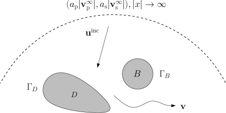
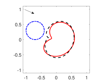
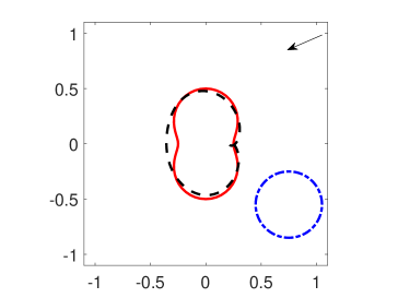
In the next section, we will show that both the modulus of compressional and shear far-field pattern have translation invariance for a shifted domain, when only the compressional or shear plane wave is used as an incident field. It implies that the inverse problem does not admit a unique solution by using the phaseless far-field patterns. Our goal is to overcome this issue by introducing a reference ball. As seen in Figure 1, an elastically rigid ball $B=\left\{x\in\mathbb{R}^{2}:|x|<R\right\}\subset\mathbb{R}^{2}$ with boundary $\Gamma_{B}$ is placed next to the obstacle $D$. The domain $B$ is called the reference ball and is used to break the translation invariance for the far-field pattern. To this end, the phaseless inverse obstacle scattering problem is stated as follows:

Problem 2 (Phaseless IOSP).

Let $B=\left\{x\in\mathbb{R}^{2}:|x|<R\right\}\subset\mathbb{R}^{2}$ be an artificially added rigid ball such that $D\cap B=\emptyset$. Given a compressional or shear incident plane wave $\boldsymbol{u}^{\rm inc}$ for a fixed angular frequency $\omega$, Lamé parameters $\lambda,\mu$, and a single incident direction $d$, the IOSP is to determine the location and shape of the boundary $\Gamma_{D}$ from the phaseless far-field data $\big{(}a_{\rm p}|\boldsymbol{v}_{\rm p}^{\infty}(\hat{x})|,a_{\rm s}|\boldsymbol{v}_{\rm s}^{\infty}(\hat{x})|\big{)},\forall\hat{x}\in\Omega$, which is generated by the scatterer $D\cup B$.

In the following, we shall introduce a system of nonlinear integral equations and develop corresponding reconstruction algorithm for solving Problem 1 and Problem 2, respectively.

3. Far-field patterns

In this section, we establish the relationship of the far-field patterns between the scattered field $\boldsymbol{v}$ and the scalar potentials $\phi,\psi$.

Denote the fundamental solution to the two-dimensional Helmholtz equation by

$$\Phi(x,y;\kappa)=\frac{\mathrm{i}}{4}H_{0}^{(1)}(\kappa|x-y|),\quad x\neq y,$$

where $H_{0}^{(1)}$ is the Hankel function of the first kind with order zero.

Theorem 3.1.

The radiating solution $\boldsymbol{v}$ to the Navier equation has the asymptotic behavior

$$\boldsymbol{v}(x)=\frac{\mathrm{e}^{\mathrm{i}\kappa_{\rm p}|x|}}{\sqrt{|x|}}\boldsymbol{v}_{\rm p}^{\infty}+\frac{\mathrm{e}^{\mathrm{i}\kappa_{\rm s}|x|}}{\sqrt{|x|}}\boldsymbol{v}_{\rm s}^{\infty}+\mathcal{O}\left(\frac{1}{|x|^{\frac{3}{2}}}\right),\quad|x|\to\infty$$

uniformly for all direction $\hat{x}$, where the vectors

$$\boldsymbol{v}_{\rm p}^{\infty}(\hat{x})=\mathrm{i}\kappa_{\rm p}\phi_{\infty}(\hat{x})\hat{x},\qquad\boldsymbol{v}_{\rm s}^{\infty}(\hat{x})=-\mathrm{i}\kappa_{\rm s}\psi_{\infty}(\hat{x})\hat{x}^{\perp}$$ (3.1)

defined on the unit circle $\Omega$ are the far-field patterns of $\boldsymbol{v}_{\rm p}$ and $\boldsymbol{v}_{\rm s}$, and the complex-valued functions $\phi_{\infty}(\hat{x})$ and $\psi_{\infty}(\hat{x})$ are the far-field patterns corresponding to $\phi$ and $\psi$.

Proof.

It follows from Green’s formula in [7, Theorem 2.5] that we have

$$\phi(x)=\int_{\Gamma_{D}}\left\{\phi(y)\frac{\partial\Phi(x,y;\kappa_{\rm p})}{\partial\nu(y)}-\frac{\partial\phi}{\partial\nu}(y)\Phi(x,y;\kappa_{\rm p})\right\}\mathrm{d}s(y),\quad x\in\mathbb{R}^{2}\setminus\overline{D}.$$

The corresponding far-field pattern is

$$\phi_{\infty}(\hat{x})=\gamma_{\kappa_{\rm p}}\int_{\Gamma_{D}}\left\{\phi(y)\frac{\partial\mathrm{e}^{-\mathrm{i}\kappa_{\rm p}\hat{x}\cdot y}}{\partial\nu(y)}-\frac{\partial\phi}{\partial\nu}(y)\mathrm{e}^{-\mathrm{i}\kappa_{\rm p}\hat{x}\cdot y}\right\}\mathrm{d}s(y),$$

where $\gamma_{\kappa_{\rm p}}={\mathrm{e}^{\mathrm{i}\pi/4}}/{\sqrt{8\kappa_{\rm p}\pi}}$. By the Helmholtz decomposition, the compressional wave can be represented by

$$\boldsymbol{v}_{\rm p}(x)=\nabla_{x}\phi(x)=\int_{\Gamma_{D}}\left\{\phi(y)\frac{\partial}{\partial\nu(y)}\big{(}\nabla_{x}\Phi(x,y;\kappa_{\rm p})\big{)}-\frac{\partial\phi}{\partial\nu}(y)\nabla_{x}\Phi(x,y;\kappa_{\rm p})\right\}\mathrm{d}s(y).$$ (3.2)

Using straight forward calculations and noting $H_{1}^{(1)}=-{H_{0}^{(1)}}^{\prime}$, we obtain

$$\nabla_{x}\Phi(x,y;\kappa_{\rm p})=\frac{-\mathrm{i}\kappa_{\rm p}}{4}H_{1}^{(1)}(\kappa_{\rm p}|x-y|)\frac{x-y}{|x-y|}.$$

With the help of the asymptotic behavior of the Hankel functions [7, eqn. (3.82)]

$$H_{n}^{(1)}(t)=\sqrt{\frac{2}{\pi t}}\rm{exp}\bigg{\{}\mathrm{i}(t-\frac{n\pi}{2}-\frac{\pi}{4})\bigg{\}}\left\{1+\mathcal{O}\left(\frac{1}{t}\right)\right\}$$

and

$$|x-y|=|x|-\hat{x}\cdot y+\mathcal{O}\left(\frac{1}{|x|}\right),$$

we derive

$$\nabla_{x}\Phi(x,y;\kappa_{\rm p})=\frac{\mathrm{e}^{\mathrm{i}\kappa_{\rm p}|x|}}{\sqrt{|x|}}\left\{\mathrm{i}\gamma_{\kappa_{\rm p}}\kappa_{\rm p}\mathrm{e}^{-\mathrm{i}\kappa_{\rm p}\hat{x}\cdot y}\hat{x}+\mathcal{O}\left(\frac{1}{|x|}\right)\right\}$$

and

$$\frac{\partial}{\partial\nu(y)}\nabla_{x}\Phi(x,y;\kappa_{\rm p})=\frac{\mathrm{e}^{\mathrm{i}\kappa_{\rm p}|x|}}{\sqrt{|x|}}\left\{\mathrm{i}\gamma_{\kappa_{\rm p}}\kappa_{\rm p}\frac{\partial\mathrm{e}^{-\mathrm{i}\kappa_{\rm p}\hat{x}\cdot y}}{\partial\nu(y)}\hat{x}+\mathcal{O}\left(\frac{1}{|x|}\right)\right\},$$

Substituting the last two equations into (3.2) yields

$$\boldsymbol{v}_{\rm p}=\frac{\mathrm{e}^{\mathrm{i}\kappa_{\rm p}|x|}}{\sqrt{|x|}}\left\{\mathrm{i}\kappa_{\rm p}\phi_{\infty}\hat{x}+\mathcal{O}\left(\frac{1}{|x|}\right)\right\}.$$

Similarly, by noting $\boldsymbol{v}_{\rm s}=\boldsymbol{\rm curl}_{x}\psi$ and

$$\boldsymbol{\rm curl}_{x}\Phi(x,y;\kappa_{\rm s})=\frac{\mathrm{i}\kappa_{\rm s}}{4}H_{1}^{(1)}(\kappa_{\rm s}|x-y|)\frac{(x-y)^{\perp}}{|x-y|},$$

we can obtain that

$$\boldsymbol{v}_{\rm s}=\frac{\mathrm{e}^{\mathrm{i}\kappa_{\rm s}|x|}}{\sqrt{|x|}}\left\{-\mathrm{i}\kappa_{\rm s}\psi_{\infty}\hat{x}^{\perp}+\mathcal{O}\left(\frac{1}{|x|}\right)\right\},$$

which completes the proof. ∎

In view of (3.1), we see that if $(a_{\rm p}\boldsymbol{v}_{\rm p}^{\infty},a_{\rm s}\boldsymbol{v}_{\rm s}^{\infty})$ or $(a_{\rm p}|\boldsymbol{v}_{\rm p}^{\infty}|,a_{\rm s}|\boldsymbol{v}_{\rm s}^{\infty}|)$ is known, then the information of far-field pattern $(a_{\rm p}\phi_{\infty},a_{\rm s}\psi_{\infty})$ or $(a_{\rm p}|\phi_{\infty}|,a_{\rm s}|\psi_{\infty}|)$ can be obtained. Hence, we may reconstruct the obstacle from the knowledge of $(a_{\rm p}\phi_{\infty},a_{\rm s}\psi_{\infty})$ and $(a_{\rm p}|\phi_{\infty}|,a_{\rm s}|\psi_{\infty}|)$ in Problem 1 and Problem 2, respectively.

The following result show the translation invariance property of the phaseless compressional and shear far-field patterns.

Theorem 3.2.

Assume that $\phi_{\infty},\psi_{\infty}$ are the far-field patterns of the scattered waves $\phi,\psi$ with incident plane wave $\boldsymbol{u}^{\rm inc}(x)=a^{\rm inc}_{\rm p}d\mathrm{e}^{{\rm i}\kappa_{\rm p}d\cdot x}+a^{\rm inc}_{\rm s}d^{\perp}\mathrm{e}^{{\rm i}\kappa_{\rm s}d\cdot x}$, where $(a^{\rm inc}_{\rm p},a^{\rm inc}_{\rm s})=(1,0)$ for the compressional incident plane wave and $(a^{\rm inc}_{\rm p},a^{\rm inc}_{\rm s})=(0,1)$ for the shear incident plane wave. For the shifted domain $D_{h}:=\{x+h:x\in D\}$ with a fixed vector $h\in\mathbb{R}^{2}$, the far-field patterns $\phi_{\infty}^{h},\psi_{\infty}^{h}$ satisfy the relations

$$\phi_{\infty}^{h}(\hat{x})=\mathrm{e}^{\mathrm{i}\kappa_{\rm p}(d-\hat{x})\cdot h}\phi_{\infty}(\hat{x}),\quad\psi_{\infty}^{h}(\hat{x})=\mathrm{e}^{\mathrm{i}(\kappa_{\rm p}d-\kappa_{\rm s}\hat{x})\cdot h}\psi_{\infty}(\hat{x}),\quad(a^{\rm inc}_{\rm p},a^{\rm inc}_{\rm s})=(1,0)$$ (3.3)

and

$$\psi_{\infty}^{h}(\hat{x})=\mathrm{e}^{\mathrm{i}\kappa_{\rm s}(d-\hat{x})\cdot h}\psi_{\infty}(\hat{x}),\quad\phi_{\infty}^{h}(\hat{x})=\mathrm{e}^{\mathrm{i}(\kappa_{\rm s}d-\kappa_{\rm p}\hat{x})\cdot h}\phi_{\infty}(\hat{x}),\quad(a^{\rm inc}_{\rm p},a^{\rm inc}_{\rm s})=(0,1).$$ (3.4)

Proof.

We only give the proof for the compressional incident plane wave case, i.e., (3.3) for $(a^{\rm inc}_{\rm p},a^{\rm inc}_{\rm s})=(1,0)$, since the other case (3.4) for $(a^{\rm inc}_{\rm p},a^{\rm inc}_{\rm s})=(0,1)$ can be proved similarly.

We assume that the solution of (2.3) is given as single-layer potentials with densities $g_{1},g_{2}$:

$$\phi(x)=\int_{\Gamma_{D}}\Phi(x,y;\kappa_{\rm p})g_{1}(y)\mathrm{d}s(y),\quad\psi(x)=\int_{\Gamma_{D}}\Phi(x,y;\kappa_{\rm s})g_{2}(y)\mathrm{d}s(y),\quad x\in\mathbb{R}^{2}\setminus\Gamma_{D}.$$ (3.5)

Letting $x\in\mathbb{R}^{2}\setminus\overline{D}$ approach the boundary $\Gamma_{D}$ in (3.5), and using the jump relation of single-layer potentials and the boundary condition of (2.3), we deduce for $x\in\Gamma_{D}$ that

$$-\frac{1}{2}g_{1}(x)+\int_{\Gamma_{D}}\frac{\partial\Phi(x,y;\kappa_{\rm p})}{\partial\nu(x)}g_{1}(y)\mathrm{d}s(y)+\int_{\Gamma_{D}}\frac{\partial\Phi(x,y;\kappa_{\rm s})}{\partial\tau(x)}g_{2}(y)\mathrm{d}s(y)=-\nu(x)\cdot\boldsymbol{u}^{\rm inc}(x)$$ (3.6)

and

$$\int_{\Gamma_{D}}\frac{\partial\Phi(x,y;\kappa_{\rm p})}{\partial\tau(x)}g_{1}(y)\mathrm{d}s(y)+\frac{1}{2}g_{2}(x)-\int_{\Gamma_{D}}\frac{\partial\Phi(x,y;\kappa_{\rm s})}{\partial\nu(x)}g_{2}(y)\mathrm{d}s(y)=-\tau(x)\cdot\boldsymbol{u}^{\rm inc}(x).$$ (3.7)

The corresponding far-field patterns can be represented as follows

$$\phi_{\infty}(\hat{x})=\gamma_{\kappa_{\rm p}}\int_{\Gamma_{D}}\mathrm{e}^{-\mathrm{i}\kappa_{\rm p}\hat{x}\cdot y}g_{1}(y)\mathrm{d}s(y),\quad\psi_{\infty}(\hat{x})=\gamma_{\kappa_{\rm s}}\int_{\Gamma_{D}}\mathrm{e}^{-\mathrm{i}\kappa_{\rm s}\hat{x}\cdot y}g_{2}(y)\mathrm{d}s(y),\quad\hat{x}\in\Omega.$$ (3.8)

Furthermore, we assume that the densities $g_{1}^{h},g_{2}^{h}$ solve the boundary integral equations (3.6)–(3.7) with $\Gamma_{D}$ replaced by $\Gamma_{D_{h}}$. We now show that if $g_{1},g_{2}$ solve (3.6)–(3.7), then

$$g_{1}^{h}(x)=\mathrm{e}^{\mathrm{i}\kappa_{\rm p}d\cdot h}g_{1}(x-h),\qquad g_{2}^{h}(x)=\mathrm{e}^{\mathrm{i}\kappa_{\rm p}d\cdot h}g_{2}(x-h)$$ (3.9)

also solve the boundary integral equations (3.6)–(3.7) with $\Gamma_{D}$ replaced by $\Gamma_{D_{h}}$. In fact, substituting above equations into the left side of (3.6)–(3.7) with $\Gamma_{D}$ replaced by $\Gamma_{D_{h}}$ and setting $\tilde{x}=x-h$, $\tilde{y}=y-h$, we get for $x\in\partial D_{h}$ that

$$-\frac{1}{2}g_{1}^{h}(x)+\int_{\Gamma_{D_{h}}}\frac{\partial\Phi(x,y;\kappa_{\rm p})}{\partial\nu(x)}g_{1}^{h}(y)\mathrm{d}s(y)+\int_{\Gamma_{D_{h}}}\frac{\partial\Phi(x,y;\kappa_{\rm s})}{\partial\tau(x)}g_{2}^{h}(y)\mathrm{d}s(y)$$

$$= \mathrm{e}^{\mathrm{i}\kappa_{\rm p}d\cdot h}\left(-\frac{1}{2}g_{1}^{h}(\tilde{x})+\int_{\Gamma_{D}}\frac{\partial\Phi(\tilde{x},\tilde{y};\kappa_{\rm p})}{\partial\nu(\tilde{x})}g_{1}^{h}(\tilde{y})\mathrm{d}s(\tilde{y})+\int_{\Gamma_{D}}\frac{\partial\Phi(\tilde{x},\tilde{y};\kappa_{\rm s})}{\partial\tau(\tilde{x})}g_{2}^{h}(\tilde{y})\mathrm{d}s(\tilde{y})\right)$$

$$= \mathrm{e}^{\mathrm{i}\kappa_{\rm p}d\cdot h}\big{(}-\nu(\tilde{x})\cdot\boldsymbol{u}^{\rm inc}(\tilde{x})\big{)}=-\nu(x)\cdot\boldsymbol{u}^{\rm inc}(x).$$

Similarly, (3.7) can be handled in the same way. Thus, the relation (3.9) follows from the fact that the system of boundary integral equations (3.6)–(3.7) for $D_{h}$ has a unique solution [26].

Combining (3.8) and (3.9), we obtain

$$\phi_{\infty}^{h}(\hat{x}) =\gamma_{\kappa_{\rm p}}\int_{\Gamma_{D_{h}}}\mathrm{e}^{-\mathrm{i}\kappa_{\rm p}\hat{x}\cdot y}g_{1}^{h}(y)\mathrm{d}s(y)$$

$$=\gamma_{\kappa_{\rm p}}\int_{\Gamma_{D_{h}}}\mathrm{e}^{-\mathrm{i}\kappa_{\rm p}\hat{x}\cdot(y-h)}\mathrm{e}^{-\mathrm{i}\kappa_{\rm p}\hat{x}\cdot h}\mathrm{e}^{\mathrm{i}\kappa_{\rm p}d\cdot h}g_{1}(y-h)\mathrm{d}s(y)=\mathrm{e}^{\mathrm{i}\kappa_{\rm p}(d-\hat{x})\cdot h}\phi_{\infty}(\hat{x})$$

and

$$\psi_{\infty}^{h}(\hat{x}) =\gamma_{\kappa_{\rm s}}\int_{\Gamma_{D_{h}}}\mathrm{e}^{-\mathrm{i}\kappa_{\rm s}\hat{x}\cdot y}g_{2}^{h}(y)\mathrm{d}s(y)$$

$$=\gamma_{\kappa_{\rm s}}\int_{\Gamma_{D_{h}}}\mathrm{e}^{-\mathrm{i}\kappa_{\rm s}\hat{x}\cdot(y-h)}\mathrm{e}^{-\mathrm{i}\kappa_{\rm s}\hat{x}\cdot h}\mathrm{e}^{\mathrm{i}\kappa_{\rm p}d\cdot h}g_{2}(y-h)\mathrm{d}s(y)=\mathrm{e}^{\mathrm{i}(\kappa_{\rm p}d-\kappa_{\rm s}\hat{x})\cdot h}\psi_{\infty}(\hat{x}),$$

which completes the proof. ∎

Theorem 3.2 implies that the compressional and shear far-field patterns are invariant under translations of the obstacle $D$ for the compressional or shear plane incident wave.

4. Nyström-type discretization for boundary integral equations

In this section, we present a Nyström-type discretization to solve the coupled system (3.6)–(3.7) . We first introduce the single-layer integral operator

$$(S_{\kappa}g)(x)=2\int_{\Gamma_{D}}\Phi(x,y;\kappa)g(y)\mathrm{d}s(y),\quad x\in\Gamma_{D},$$

and the corresponding far-field integral operator

$$(S_{\kappa}^{\infty}g)(\hat{x})=\gamma_{\kappa}\int_{\Gamma_{D}}\mathrm{e}^{-\mathrm{i}\kappa\hat{x}\cdot y}g(y)\mathrm{d}s(y),\quad\hat{x}\in\Omega.$$

In addition, we need to introduce the normal derivative boundary integral operator

$$(K_{\kappa}g)(x)=2\int_{\Gamma_{D}}\frac{\partial\Phi(x,y;\kappa)}{\partial\nu(x)}g(y)\mathrm{d}s(y),\qquad x\in\Gamma_{D},$$

and the tangential derivative boundary integral operator

$$(H_{\kappa}g)(x)=2\int_{\Gamma_{D}}\frac{\partial\Phi(x,y;\kappa)}{\partial\tau(x)}g(y)\mathrm{d}s(y),\qquad x\in\Gamma_{D}.$$

Then, the coupled boundary integral equations (3.6)–(3.7) can be rewritten in the operator form

$$-g_{1}+K_{\kappa_{\rm p}}g_{1}+H_{\kappa_{\rm s}}g_{2}=2f_{1},$$ (4.1)

$$H_{\kappa_{\rm p}}g_{1}+g_{2}-K_{\kappa_{\rm s}}g_{2}=2f_{2}.$$ (4.2)

The corresponding far-field patterns of (3.8) can be represented as follows

$$\phi_{\infty}(\hat{x})=(S_{\kappa_{\rm p}}^{\infty}g_{1})(\hat{x}),\quad\psi_{\infty}(\hat{x})=(S_{\kappa_{\rm s}}^{\infty}g_{2})(\hat{x}),\qquad\hat{x}\in\Omega.$$

4.1. Parametrization

For simplicity, the boundary $\Gamma_{D}$ is assumed to be a star-shaped curve with the parametric form

$$\Gamma_{D}=\{p(\hat{x})=c+r(\hat{x})\hat{x}:~{}c=(c_{1},c_{2})^{\top},\ \hat{x}\in\Omega\},$$

where $\Omega=\{\hat{x}(t)=(\cos t,\sin t)^{\top}:~{}0\leq t<2\pi\}$. We introduce the parameterized integral operators which are still denoted by $S_{\kappa}$, $S_{\kappa}^{\infty}$, $K_{\kappa}$, and $H_{\kappa}$ for convenience, i.e.,

$$\big{(}S_{\kappa}(p,\varphi_{j})\big{)}(t) =\frac{\mathrm{i}}{2}\int_{0}^{2\pi}H_{0}^{(1)}(\kappa|p(t)-p(\varsigma)|)\varphi_{j}(\varsigma)\mathrm{d}\varsigma,$$

$$\big{(}S^{\infty}_{\kappa}(p,\varphi_{j})\big{)}(t) =\gamma_{\kappa}\int_{0}^{2\pi}\mathrm{e}^{-\mathrm{i}\kappa\hat{x}(t)\cdot p(\varsigma)}\varphi_{j}(\varsigma)\mathrm{d}\varsigma,$$

$$\big{(}K_{\kappa}(p,\varphi_{j})\big{)}(t) =\frac{1}{G(t)}\int_{0}^{2\pi}\widetilde{K}(t,\varsigma;\kappa)\varphi_{j}(\varsigma)\mathrm{d}\varsigma,$$

$$\big{(}H_{\kappa}(p,\varphi_{j})\big{)}(t) =\frac{1}{G(t)}\int_{0}^{2\pi}\widetilde{H}(t,\varsigma;\kappa)\varphi_{j}(\varsigma)\mathrm{d}\varsigma,$$

where $\varphi_{j}(\varsigma)=G(\varsigma)g_{j}(p(\varsigma))$, $j=1,2$, $G(\varsigma):=|p^{\prime}(\varsigma)|=\sqrt{(r^{\prime}(\varsigma))^{2}+r^{2}(\varsigma)}$ is the Jacobian of the transformation,

$$\widetilde{K}(t,\varsigma;\kappa) =\frac{\mathrm{i}\kappa}{2}n(t)\cdot[p(\varsigma)-p(t)]\frac{H_{1}^{(1)}(\kappa|p(t)-p(\varsigma)|)}{|p(t)-p(\varsigma)|},$$

$$\widetilde{H}(t,\varsigma;\kappa) =\frac{\mathrm{i}\kappa}{2}n(t)^{\perp}\cdot[p(\varsigma)-p(t)]\frac{H_{1}^{(1)}(\kappa|p(t)-p(\varsigma)|)}{|p(t)-p(\varsigma)|},$$

and

$$n(t)=\nu(x(t))|p^{\prime}(t)|=\big{(}p^{\prime}_{2}(t),-p^{\prime}_{1}(t)\big{)},\quad n(t)^{\perp}=\tau(x(t))|p^{\prime}(t)|=\big{(}p^{\prime}_{1}(t),p^{\prime}_{2}(t)\big{)}.$$

Hence, equations (4.1)–(4.2) can be reformulated as the parametrized integral equations

$$-\varphi_{1}+K_{\kappa_{\rm p}}(p,\varphi_{1})G+H_{\kappa_{\rm s}}(p,\varphi_{2})G =w_{1},$$ (4.3)

$$\varphi_{2}+H_{\kappa_{\rm p}}(p,\varphi_{1})G-K_{\kappa_{\rm s}}(p,\varphi_{2})G =w_{2},$$ (4.4)

where $w_{j}=2(f_{j}\circ p)G$, $j=1,2$.

4.2. Discretization

We adopt the Nyström method for the discretization of the boundary integrals. We refer to [21] for an application of the Nyström method to solve the acoustic wave scattering problem by using a hypersingular integral equation.

The kernel $\widetilde{K}$ of the parameterized normal derivative integral operator can be written in the form of

$$\widetilde{K}(t,\varsigma;\kappa)=\widetilde{K}_{1}(t,\varsigma;\kappa)\ln\Big{(}4\sin^{2}\frac{t-\varsigma}{2}\Big{)}+\widetilde{K}_{2}(t,\varsigma;\kappa),$$

where

$$\widetilde{K}_{1}(t,\varsigma;\kappa) =\frac{\kappa}{2\pi}n(t)\cdot\big{[}p(t)-p(\varsigma)\big{]}\frac{J_{1}(\kappa|p(t)-p(\varsigma)|)}{|p(t)-p(\varsigma)|},$$

$$\widetilde{K}_{2}(t,\varsigma;\kappa) =\widetilde{K}(t,\varsigma;\kappa)-\widetilde{K}_{1}(t,\varsigma;\kappa)\ln\Big{(}4\sin^{2}\frac{t-\varsigma}{2}\Big{)}.$$

It can be shown that the diagonal terms are

$$\widetilde{K}_{1}(t,t;\kappa)=0,\qquad\widetilde{K}_{2}(t,t;\kappa)=\frac{1}{2\pi}\frac{n(t)\cdot p^{\prime\prime}(t)}{|p^{\prime}(t)|^{2}}.$$

Noting $H_{1}^{(1)}=J_{1}+\mathrm{i}Y_{1}$, where $J_{1}$ and $Y_{1}$ are the Bessel and Neumann functions of order one, and using the power series [7, eqns. (3.74) and (3.75)]

$$J_{1}(z) :=\sum_{k=0}^{\infty}\frac{(-1)^{k}}{k!(k+1)!}\Big{(}\frac{z}{2}\Big{)}^{2k+1}$$

$$Y_{1}(z) :=\frac{2}{\pi}\Big{\{}\ln\frac{z}{2}+C\Big{\}}J_{1}(z)-\frac{2}{\pi}\frac{1}{z}-\frac{1}{\pi}\sum_{k=0}^{\infty}\frac{(-1)^{k}}{k!(k+1)!}\Big{\{}\psi(k+1)+\psi(k)\Big{\}}\Big{(}\frac{z}{2}\Big{)}^{2k+1}$$

where $\psi(k)=\sum_{m=1}^{k}\frac{1}{m}$ with definition $\psi(0)=0$ and Euler’s constant $C=0.57721\cdots$, we can split the kernel $\widetilde{H}$ of the parameterized tangential derivative integral operator into

$$\widetilde{H}(t,\varsigma;\kappa)=\widetilde{H}_{1}(t,\varsigma;\kappa)\frac{1}{\sin(\varsigma-t)}+\widetilde{H}_{2}(t,\varsigma;\kappa)\ln\Big{(}4\sin^{2}\frac{t-\varsigma}{2}\Big{)}+\widetilde{H}_{3}(t,\varsigma;\kappa),$$

where the functions

$$\widetilde{H}_{1}(t,\varsigma;\kappa) =\frac{1}{\pi}n(t)^{\perp}\cdot\big{[}p(\varsigma)-p(t)\big{]}\frac{\sin(\varsigma-t)}{|p(t)-p(\varsigma)|^{2}},$$

$$\widetilde{H}_{2}(t,\varsigma;\kappa) =\frac{\kappa}{2\pi}n(t)^{\perp}\cdot\big{[}p(t)-p(\varsigma)\big{]}\frac{J_{1}(\kappa|p(t)-p(\varsigma)|)}{|p(t)-p(\varsigma)|},$$

$$\widetilde{H}_{3}(t,\varsigma;\kappa) =\widetilde{H}(t,\varsigma;\kappa)-\widetilde{H}_{1}(t,\varsigma;\kappa)\frac{1}{\sin(\varsigma-t)}-\widetilde{H}_{2}(t,\varsigma;\kappa)\ln\Big{(}4\sin^{2}\frac{t-\varsigma}{2}\Big{)}$$

are analytic with diagonal entries given by

$$\widetilde{H}_{1}(t,t;\kappa)=\frac{1}{\pi},\quad\widetilde{H}_{2}(t,t;\kappa)=0,\quad\widetilde{H}_{3}(t,t;\kappa)=0.$$

Let $\varsigma_{j}^{(n)}:=\pi j/n$, $j=0,\cdots,2n-1$ be an equidistant set of quadrature points. For the singular integrals, we employ the following quadrature rules via the trigonometric interpolation

$$\int_{0}^{2\pi}\ln\Big{(}4\sin^{2}\frac{t-\varsigma}{2}\Big{)}f(\varsigma)\mathrm{d}\varsigma\approx\sum_{j=0}^{2n-1}R_{j}^{(n)}(t)f(\varsigma_{j}^{(n)}),$$ (4.5)

$$\int_{0}^{2\pi}\frac{f(\varsigma)}{\sin(\varsigma-t)}\mathrm{d}\varsigma\approx\sum_{j=0}^{2n-1}T_{j}^{(n)}(t)f(\varsigma_{j}^{(n)}),$$ (4.6)

where the quadrature weights are given by

$$R_{j}^{(n)}(t)=-\frac{2\pi}{n}\sum_{m=1}^{n-1}\frac{1}{m}\cos\Big{[}m(t-\varsigma_{j}^{(n)})\Big{]}-\frac{\pi}{n^{2}}\cos\Big{[}n(t-\varsigma_{j}^{(n)})\Big{]}$$ (4.7)

and

$$T_{j}^{(n)}(t)=\begin{cases}\displaystyle-\frac{2\pi}{n}\sum_{m=0}^{(n-3)/2}\sin\Big{[}(2m+1)(t-\varsigma_{j}^{(n)})\Big{]}-\frac{\pi}{n}\sin\Big{[}n(t-\varsigma_{j}^{(n)})\Big{]},~{}&n=1,3,5,\cdots,\\ \displaystyle-\frac{2\pi}{n}\sum_{m=0}^{n/2-1}\sin\Big{[}(2m+1)(t-\varsigma_{j}^{(n)})\Big{]},~{}&n=2,4,6,\cdots.\end{cases}$$

Using the Lagrange basis for the trigonometric interpolation [24, eqn. (11.12)]), we derive the weight $T_{j}^{(n)}$ by calculating the integrals

$$\int_{0}^{2\pi}\frac{\cos k\varsigma}{\sin\varsigma}\mathrm{d}\varsigma=0,\quad k=0,1,2,\cdots,\quad \int_{0}^{2\pi}\frac{\sin k\varsigma}{\sin\varsigma}\mathrm{d}\varsigma=\begin{cases}2\pi,~{}&k=1,3,5\cdots,\\ 0,~{}&k=2,4,6,\cdots,\end{cases}$$

in the sense of Cauchy principal value. The details of (4.7) can be found in [24]. For the smooth integrals, we simply use the trapezoidal rule

$$\int_{0}^{2\pi}f(\varsigma)\mathrm{d}\varsigma\approx\frac{\pi}{n}\sum_{j=0}^{2n-1}f(\varsigma_{j}^{(n)}).$$ (4.8)

By (4.5) and (4.6), the full discretization of (4.3)–(4.4) can be deduced as

$$w_{1,i}^{(n)}= -\varphi^{(n)}_{1,i}+\sum_{j=0}^{2n-1}\left(R_{|i-j|}^{(n)}\widetilde{K}_{1}(\varsigma_{i}^{(n)},\varsigma_{j}^{(n)};\kappa_{\rm p})+\frac{\pi}{n}\widetilde{K}_{2}(\varsigma_{i}^{(n)},\varsigma_{j}^{(n)};\kappa_{\rm p})\right)\varphi_{1,j}^{(n)}$$

$$+\sum_{j=0}^{2n-1}\left(-T_{i-j}^{(n)}\widetilde{H}_{1}(\varsigma_{i}^{(n)},\varsigma_{j}^{(n)};\kappa_{\rm s})+R_{|i-j|}^{(n)}\widetilde{H}_{2}(\varsigma_{i}^{(n)},\varsigma_{j}^{(n)};\kappa_{\rm s})+\frac{\pi}{n}\widetilde{H}_{3}(\varsigma_{i}^{(n)},\varsigma_{j}^{(n)};\kappa_{\rm s})\right)\varphi_{2,j}^{(n)},$$

$$w_{2,i}^{(n)}= \varphi^{(n)}_{2,i}+\sum_{j=0}^{2n-1}\left(-T_{i-j}^{(n)}\widetilde{H}_{1}(\varsigma_{i}^{(n)},\varsigma_{j}^{(n)};\kappa_{\rm p})+R_{|i-j|}^{(n)}H_{2}(\varsigma_{i}^{(n)},\varsigma_{j}^{(n)};\kappa_{\rm p})+\frac{\pi}{n}\widetilde{H}_{3}(\varsigma_{i}^{(n)},\varsigma_{j}^{(n)};\kappa_{\rm p})\right)\varphi_{1,j}^{(n)}$$

$$-\sum_{j=0}^{2n-1}\left(R_{|i-j|}^{(n)}\widetilde{K}_{1}(\varsigma_{i}^{(n)},\varsigma_{j}^{(n)};\kappa_{\rm s})+\frac{\pi}{n}\widetilde{K}_{2}(\varsigma_{i}^{(n)},\varsigma_{j}^{(n)};\kappa_{\rm s})\right)\varphi_{2,j}^{(n)},$$

where $w_{l,i}^{(n)}=w_{l}(\varsigma_{i}^{(n)})$, $\varphi_{l,j}^{(n)}=\varphi_{l}(\varsigma_{j}^{(n)})$ for $i,j=0,\cdots,2n-1$, $l=1,2$, and

$$R_{j}^{(n)} :=R_{j}^{(n)}(0)=-\frac{2\pi}{n}\sum_{m=1}^{n-1}\frac{1}{m}\cos\frac{mj\pi}{n}-\frac{(-1)^{j}\pi}{n^{2}},$$

$$T_{j}^{(n)} :=T_{j}^{(n)}(0)=\frac{2\pi}{n}\sum_{m=0}^{\tilde{n}}\sin\frac{(2m+1)j\pi}{n},\qquad\tilde{n}=\begin{cases}(n-3)/2,&n=1,3,5,\cdots,\\ n/2-1,&n=2,4,6,\cdots.\end{cases}$$

5. Reconstruction methods

In this section, we introduce a system of nonlinear equations and develop corresponding reconstruction methods for Problem 1 and Problem 2, respectively.

5.1. The phased IOSP

On $\Gamma_{D}$, it follows from the boundary integral equations (4.1)–(4.2) that the field equations are

$$-g_{1}+K_{\kappa_{\rm p}}g_{1}+H_{\kappa_{\rm s}}g_{2}=2f_{1},$$ (5.1)

$$H_{\kappa_{\rm p}}g_{1}+g_{2}-K_{\kappa_{\rm s}}g_{2}=2f_{2}.$$ (5.2)

The data equation is given by

$$a_{\rm p}S^{\infty}_{\kappa_{\rm p}}g_{1}+a_{\rm s}S^{\infty}_{\kappa_{\rm s}}g_{2}=a_{\rm p}\phi_{\infty}+a_{\rm s}\psi_{\infty}.$$ (5.3)

The field equations and data equation (5.1)–(5.3) can be reformulated as the parametrized integral equations

$$-\varphi_{1}+K_{\kappa_{\rm p}}(p,\varphi_{1})G+H_{\kappa_{\rm s}}(p,\varphi_{2})G =w_{1},$$ (5.4)

$$\varphi_{2}+H_{\kappa_{\rm p}}(p,\varphi_{1})G-K_{\kappa_{\rm s}}(p,\varphi_{2})G =w_{2},$$ (5.5)

$$a_{\rm p}S^{\infty}_{\kappa_{\rm p}}(p,\varphi_{1})+a_{\rm s}S^{\infty}_{\kappa_{\rm s}}(p,\varphi_{2})=a_{\rm p}\phi_{\infty} +a_{\rm s}\psi_{\infty},$$ (5.6)

where $w_{j}=2(f_{j}\circ p)G$, $j=1,2$.

In the reconstruction process, when an approximation of the boundary $\Gamma_{D}$ is available, the field equations (5.4)–(5.5) are solved for the densities $g_{1}$ and $g_{2}$. Once the approximated densities $g_{1}$ and $g_{2}$ are computed, the update of the boundary $\Gamma_{D}$ can be obtained by solving the linearized data equation (5.6) with respect to $\Gamma_{D}$.

5.1.1. Iterative scheme

The linearization of (5.6) with respect to $p$ requires the Fréchet derivative of the parameterized integral operator $S_{\kappa}^{\infty}$, which can be explicitly calculated as follows

$$\Big{(}{S_{\kappa}^{\infty}}^{\prime}[p;\varphi]q\Big{)}(t)= -\mathrm{i}\kappa\gamma_{\kappa}\int_{0}^{2\pi}\mathrm{e}^{-\mathrm{i}\kappa\hat{x}(t)\cdot p(\varsigma)}\hat{x}(t)\cdot q(\varsigma)\varphi(\varsigma)\mathrm{d}\varsigma$$

$$= -\mathrm{i}\kappa\gamma_{\kappa}\int_{0}^{2\pi}\exp\Big{(}-\mathrm{i}\kappa\big{(}c_{1}\cos t+c_{2}\sin t+r(\varsigma)\cos(t-\varsigma)\big{)}\Big{)}$$

$$\qquad\quad\times\Big{(}\Delta c_{1}\cos t+\Delta c_{2}\sin t+\Delta r(\varsigma)\cos(t-\varsigma)\Big{)}\varphi(\varsigma)\,\mathrm{d}\varsigma,$$ (5.7)

where

$$q(\varsigma)=(\Delta c_{1},\Delta c_{2})+\Delta r(\varsigma)(\cos\varsigma,\sin\varsigma)$$

gives the update of the boundary $\Gamma_{D}$. Then, the linearization of (5.6) leads to

$$a_{\rm p}{S_{\kappa_{\rm p}}^{\infty}}^{\prime}[p;\varphi_{1}]q+a_{\rm s}{S_{\kappa_{\rm s}}^{\infty}}^{\prime}[p;\varphi_{2}]q=w,$$ (5.8)

where

$$w:= a_{\rm p}\Big{(}\phi_{\infty}-S^{\infty}_{\kappa_{\rm p}}(p,\varphi_{1})\Big{)}+a_{\rm s}\Big{(}\psi_{\infty}-S^{\infty}_{\kappa_{\rm s}}(p,\varphi_{2})\Big{)}.$$

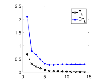
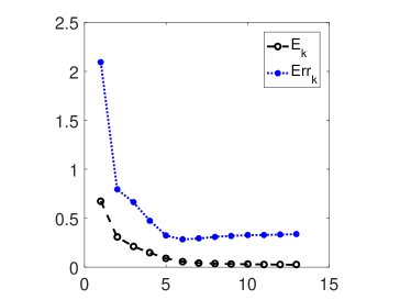
As usual, a stopping criteria is necessary to terminate the iteration. For our iterative procedure, the following relative error estimator is used

$${\rm E}_{k}:=\frac{\left\|a_{\rm p}\Big{(}\phi_{\infty}-S^{\infty}_{\kappa_{\rm p}}(p^{(k)},\varphi_{1})\Big{)}+a_{\rm s}\Big{(}\psi_{\infty}-S^{\infty}_{\kappa_{\rm s}}(p^{(k)},\varphi_{2})\Big{)}\right\|_{L^{2}}}{\big{\|}a_{\rm p}\phi_{\infty}+a_{\rm s}\psi_{\infty}\big{\|}_{L^{2}}}\leq\epsilon,$$ (5.9)

where $\epsilon$ is a user-specified small positive constant depending on the noise level and $p^{(k)}$ is the $k$th approximation of the boundary $\Gamma_{D}$.

We are now in a position to present the iterative algorithm for the inverse obstacle scattering problem with phased far-field data as Algorithm I.

Algorithm I: Iterative algorithm for the phased IOSP
Step 1	Send an incident plane wave $\boldsymbol{u}^{\rm inc}$ with fixed $\omega,\lambda,\mu$, and a fixed incident direction $d\in\Omega$, and then collect the corresponding far-field data $\phi_{\infty}$ or $\psi_{\infty}$ for the scatterer $D$;
Step 2	Select an initial star-like curve $\Gamma^{(0)}$ for the boundary $\Gamma_{D}$ and the error tolerance $\epsilon$. Set $k=0$;
Step 3	For the curve $\Gamma^{(k)}$, compute the densities $\varphi_{1}$ and $\varphi_{2}$ from (5.4)–(5.5);
Step 4	Solve (5.8) to obtain the updated approximation $\Gamma^{(k+1)}:=\Gamma^{(k)}+q$ and evaluate the error $E_{k+1}$ defined in (5.9);
Step 5	If $E_{k+1}\geq\epsilon$, then set $k=k+1$ and go to Step 3. Otherwise, the current approximation $\Gamma^{(k+1)}$ is taken to be the final reconstruction of $\Gamma_{D}$.

5.1.2. Discretization

We use the Nyström method which is described in Section 4 for the full discretizations of (5.4)–(5.5). Now we discuss the discretization of the linearized equation (5.8) and obtain the update by using least squares with Tikhonov regularization [23]. As for a finite dimensional space to approximate the radial function $r$ and its update $\Delta r$, we choose the space of trigonometric polynomials of the form

$$\Delta r(\tau)=\sum_{m=0}^{M}\alpha_{m}\cos{m\tau}+\sum_{m=1}^{M}\beta_{m}\sin{m\tau},$$ (5.10)

where the integer $M>1$ denotes the truncation number. For simplicity, we reformulate the equation (5.8) by introducing the following definitions

$$L_{1}(t,\varsigma;\kappa,\varphi):=-\mathrm{i}\kappa\gamma_{\kappa}\exp\left\{-\mathrm{i}\kappa\Big{(}c_{1}\cos t+c_{2}\sin t+r(\varsigma)\cos(t-\varsigma)\Big{)}\right\}\cos t~{}\varphi(\varsigma),$$

$$L_{2}(t,\varsigma;\kappa,\varphi):=-\mathrm{i}\kappa\gamma_{\kappa}\exp\left\{-\mathrm{i}\kappa\Big{(}c_{1}\cos t+c_{2}\sin t+r(\varsigma)\cos(t-\varsigma)\Big{)}\right\}\sin t~{}\varphi(\varsigma),$$

$$L_{3,m}(t,\varsigma;\kappa,\varphi):=-\mathrm{i}\kappa\gamma_{\kappa}\exp\left\{-\mathrm{i}\kappa\Big{(}c_{1}\cos t+c_{2}\sin t+r(\varsigma)\cos(t-\varsigma)\Big{)}\right\}\cos(t-\varsigma)\cos m\varsigma~{}\varphi(\varsigma),$$

$$L_{4,m}(t,\varsigma;\kappa,\varphi):=-\mathrm{i}\kappa\gamma_{\kappa}\exp\left\{-\mathrm{i}\kappa\Big{(}c_{1}\cos t+c_{2}\sin t+r(\varsigma)\cos(t-\varsigma)\Big{)}\right\}\cos(t-\varsigma)\sin m\varsigma~{}\varphi(\varsigma).$$

Combining (5.7)–(5.8) and using the trapezoidal rule (4.8), we get the discretized linear system

$$a_{\rm p} \bigg{(}\sum_{l=1}^{2}B_{l}^{c}(\varsigma_{i}^{(\bar{n})};\kappa_{\rm p},\varphi_{1})\Delta c_{l}+\sum_{m=0}^{M}\alpha_{m}B_{1,m}^{r}(\varsigma_{i}^{(\bar{n})};\kappa_{\rm p},\varphi_{1})+\sum_{m=1}^{M}\beta_{m}B_{2,m}^{r}(\varsigma_{i}^{(\bar{n})};\kappa_{\rm p},\varphi_{1})\bigg{)}$$

$$+a_{\rm s}\bigg{(}\sum_{l=1}^{2}B_{j}^{c}(\varsigma_{i}^{(\bar{n})};\kappa_{\rm s},\varphi_{2})\Delta c_{l}+\sum_{m=0}^{M}\alpha_{m}B_{1,m}^{r}(\varsigma_{i}^{(\bar{n})};\kappa_{\rm s},\varphi_{2})+\sum_{m=1}^{M}\beta_{m}B_{2,m}^{r}(\varsigma_{i}^{(\bar{n})};\kappa_{\rm s},\varphi_{2})\bigg{)}$$

$$\hskip 56.9055pt=w(\varsigma_{i}^{(\bar{n})})$$ (5.11)

to determine the real coefficients $\Delta c_{1}$, $\Delta c_{2}$, $\alpha_{m}$, and $\beta_{m}$, where

$$B_{l}^{c}(\varsigma_{i}^{(\bar{n})};\kappa,\varphi)=\frac{\pi}{n}\sum_{j=0}^{2n-1}L_{l}(\varsigma_{i}^{(\bar{n})},\varsigma_{j}^{(n)};\kappa,\varphi),\quad l=1,2,$$

and

$$B_{1,m}^{r}(\varsigma_{i}^{(\bar{n})};\kappa,\varphi) =\frac{\pi}{n}\sum_{j=0}^{2n-1}L_{3,m}(\varsigma_{i}^{(\bar{n})},\varsigma_{j}^{(n)};\kappa,\varphi),$$

$$B_{2,m}^{r}(\varsigma_{i}^{(\bar{n})};\kappa,\varphi) =\frac{\pi}{n}\sum_{j=0}^{2n-1}L_{4,m}(\varsigma_{i}^{(\bar{n})},\varsigma_{j}^{(n)};\kappa,\varphi).$$

In general, $2M+1\ll 2n$, and due to the ill-posedness, the overdetermined system (5.1.2) is solved via the Tikhonov regularization. Hence the linear system (5.1.2) is reformulated into minimizing the following function

$$\sum_{i=0}^{2n-1}\Bigg{|}a_{\rm p}\bigg{(}\sum_{l=1}^{2}B_{l}^{c}(\varsigma_{i}^{(\bar{n})};\kappa_{\rm p},\varphi_{1})\Delta c_{l}+\sum_{m=0}^{M}\alpha_{m}B_{1,m}^{r}(\varsigma_{i}^{(\bar{n})};\kappa_{\rm p},\varphi_{1})+\sum_{m=1}^{M}\beta_{m}B_{2,m}^{r}(\varsigma_{i}^{(\bar{n})};\kappa_{\rm p},\varphi_{1})\bigg{)}$$

$$\qquad+a_{\rm s}\bigg{(}\sum_{l=1}^{2}B_{j}^{c}(\varsigma_{i}^{(\bar{n})};\kappa_{\rm s},\varphi_{2})\Delta c_{l}+\sum_{m=0}^{M}\alpha_{m}B_{1,m}^{r}(\varsigma_{i}^{(\bar{n})};\kappa_{\rm s},\varphi_{2})+\sum_{m=1}^{M}\beta_{m}B_{2,m}^{r}(\varsigma_{i}^{(\bar{n})};\kappa_{\rm s},\varphi_{2})\bigg{)}$$

$$\qquad-w(\varsigma_{i}^{(\bar{n})})\Bigg{|}^{2}+\lambda\bigg{(}|\Delta c_{1}|^{2}+|\Delta c_{2}|^{2}+2\pi\Big{[}\alpha_{0}^{2}+\frac{1}{2}\sum_{m=1}^{M}(1+m^{2})^{2}(\alpha_{m}^{2}+\beta_{m}^{2})\Big{]}\bigg{)},$$ (5.12)

where $\lambda>0$ is a regularization parameter. It is easy to show that the minimizer of (5.12) is the solution of the system

$$\lambda I\xi+\Re(\widetilde{B}^{*}\widetilde{B})\xi=\Re(\widetilde{B}^{*}\widetilde{w}),$$ (5.13)

where

$$\widetilde{B}=\Big{(} a_{\rm p}B_{1}^{c}(:,\kappa_{\rm p},\varphi_{1})+a_{\rm s}B_{1}^{c}(:,\kappa_{\rm s},\varphi_{2}),a_{\rm p}B_{2}^{c}(:,\kappa_{\rm p},\varphi_{1})+a_{\rm s}B_{2}^{c}(:,\kappa_{\rm s},\varphi_{2}),$$

$$a_{\rm p}B_{1,0}^{r}(:,\kappa_{\rm p},\varphi_{1})+a_{\rm s}B_{1,0}^{r}(:,\kappa_{\rm s},\varphi_{2}),\cdots,a_{\rm p}B_{1,M}^{r}(:,\kappa_{\rm p},\varphi_{1})+a_{\rm s}B_{1,M}^{r}(:,\kappa_{\rm s},\varphi_{2}),$$

$$a_{\rm p}B_{2,1}^{r}(:,\kappa_{\rm p},\varphi_{1})+a_{\rm s}B_{2,1}^{r}(:,\kappa_{\rm s},\varphi_{2}),\cdots,a_{\rm p}B_{2,M}^{r}(:,\kappa_{\rm p},\varphi_{1})+a_{\rm s}B_{2,M}^{r}(:,\kappa_{\rm s},\varphi_{2})\Big{)}_{(2n)\times(2M+3)}$$

and

$$\xi=(\Delta c_{1},\Delta c_{2},\alpha_{0},\cdots,\alpha_{M},\beta_{1},\cdots,\beta_{M})^{\top},$$

$$\widetilde{I}=\mathrm{diag}\{1,1,2\pi,\pi(1+1^{2})^{2},\cdots,\pi(1+M^{2})^{2},\pi(1+1^{2})^{2},\cdots,\pi(1+M^{2})^{2}\},$$

$$\widetilde{w}=(w(\tau_{0}^{(n)}),\cdots,w(\tau_{2n-1}^{(n)}))^{\top}.$$

Thus, we obtain the new approximation

$$p^{new}(\hat{x})=(c+\Delta c)+\big{(}r(\hat{x})+\Delta r(\hat{x})\big{)}\hat{x}.$$

5.2. The phaseless IOSP

To incorporate the reference ball, we find the solution of (2.3) with $D$ replaced by $D\cup B$ in the form of single-layer potentials with densities $g_{1,\sigma}$ and $g_{2,\sigma}$:

$$\phi(x)=\sum_{\sigma}\int_{\Gamma_{\sigma}}\Phi(x,y;\kappa_{\rm p})g_{1,\sigma}(y)\mathrm{d}s(y),\quad\psi(x)=\sum_{\sigma}\int_{\Gamma_{\sigma}}\Phi(x,y;\kappa_{\rm s})g_{2,\sigma}(y)\mathrm{d}s(y),$$ (5.14)

for $x\in\mathbb{R}^{2}\setminus\Gamma_{D\cup B}$, where $\sigma=D,B$. We introduce integral operators

$$(K_{\kappa}^{\sigma,\varrho}g)(x)=2\int_{\Gamma_{\sigma}}\frac{\partial\Phi(x,y;\kappa)}{\partial\nu(x)}g(y)\mathrm{d}s(y),\quad x\in\Gamma_{\varrho},$$

$$(H_{\kappa}^{\sigma,\varrho}g)(x)=2\int_{\Gamma_{\sigma}}\frac{\partial\Phi(x,y;\kappa)}{\partial\tau(x)}g(y)\mathrm{d}s(y),\quad x\in\Gamma_{\varrho},$$

and the corresponding far-field pattern

$$(S_{\kappa,\sigma}^{\infty}g)(\hat{x})=\gamma_{\kappa}\int_{\Gamma_{\sigma}}\mathrm{e}^{-\mathrm{i}\kappa\hat{x}\cdot y}g(y)\mathrm{d}s(y),\quad\hat{x}\in\Omega,$$

where $\varrho=D,B$. Letting $x\in\mathbb{R}^{2}\setminus\overline{D\cup B}$ approach the boundary $\Gamma_{D}$ and $\Gamma_{B}$ respectively in (5.14), and using the jump relation of single-layer potentials and the boundary condition of (2.3) for $\Gamma_{D}\cup\Gamma_{B}$, we deduce the field equations in the operator form

$$-g_{1,D}+\sum_{\sigma}K^{\sigma,D}_{\kappa_{\rm p}}g_{1,\sigma}+\sum_{\sigma}H^{\sigma,D}_{\kappa_{\rm s}}g_{2,\sigma}=2f_{1}\quad{\rm on}~{}\Gamma_{D},$$ (5.15)

$$g_{2,D}+\sum_{\sigma}H^{\sigma,D}_{\kappa_{\rm p}}g_{1,\sigma}-\sum_{\sigma}K^{\sigma,D}_{\kappa_{\rm s}}g_{2,\sigma}=2f_{2}\quad{\rm on}~{}\Gamma_{D},$$ (5.16)

$$-g_{1,B}+\sum_{\sigma}K^{\sigma,B}_{\kappa_{\rm p}}g_{1,\sigma}+\sum_{\sigma}H^{\sigma,B}_{\kappa_{\rm s}}g_{2,\sigma}=2f_{1}\quad{\rm on}~{}\Gamma_{B},$$ (5.17)

$$g_{2,B}+\sum_{\sigma}H^{\sigma,B}_{\kappa_{\rm p}}g_{1,\sigma}-\sum_{\sigma}K^{\sigma,B}_{\kappa_{\rm s}}g_{2,\sigma}=2f_{2}\quad{\rm on}~{}\Gamma_{B}.$$ (5.18)

The phaseless data equation can be written as

$$a_{\rm p}\bigg{|}\sum_{\sigma}S^{\infty}_{\kappa_{\rm p},\sigma}g_{1,\sigma}\bigg{|}^{2}+a_{\rm s}\bigg{|}\sum_{\sigma}S^{\infty}_{\kappa_{\rm s},\sigma}g_{2,\sigma}\bigg{|}^{2}=a_{\rm p}|\phi_{\infty}|^{2}+a_{\rm s}|\psi_{\infty}|^{2}.$$ (5.19)

In the reconstruction process, for a given approximated boundary $\Gamma_{D}$, the field equations (5.15)–(5.18) can be solved for the densities $g_{1,\sigma}$ and $g_{2,\sigma}$. Once $g_{1,\sigma}$ and $g_{2,\sigma}$ are computed, the update of the boundary $\Gamma_{D}$ can be obtained by linearizing (5.19) with respect to $\Gamma_{D}$.

5.2.1. Parametrization and iterative scheme

For simplicity, the boundary $\Gamma_{D}$ and $\Gamma_{B}$ are assumed to be star-shaped curves with the parametric forms

$$\Gamma_{D}=\{p_{D}(\hat{x})=c+r(\hat{x})\hat{x}:~{}c=(c_{1},c_{2})^{\top},\ \hat{x}\in\Omega\},$$

$$\Gamma_{B}=\{p_{B}(\hat{x})=b+R\hat{x}:~{}b=(b_{1},b_{2})^{\top},\ \hat{x}\in\Omega\},$$

where $\Omega=\{\hat{x}(t)=(\cos t,\sin t)^{\top}:~{}0\leq t<2\pi\}$. Using the parametric forms of the boundaries $\Gamma_{D}$ and $\Gamma_{B}$, we introduce the parameterized integral operators which are still represented by $S_{\kappa}$, $S_{\kappa}^{\infty}$, $K_{\kappa}$, and $H_{\kappa}$ for convenience, i.e.,

$$\big{(}S_{\kappa}^{\sigma,\varrho}\varphi_{j,\sigma}\big{)}(t)=\frac{\mathrm{i}}{2}\int_{0}^{2\pi}H_{0}^{(1)}(\kappa|p_{\varrho}(t)-p_{\sigma}(\varsigma)|)\varphi_{j,\sigma}(\varsigma)\mathrm{d}\varsigma,$$

$$\big{(}S^{\infty}_{\kappa}(p,\varphi_{j,\sigma})\big{)}(t)=\gamma_{\kappa}\int_{0}^{2\pi}\mathrm{e}^{-\mathrm{i}\kappa\hat{x}(t)\cdot p(\varsigma)}\varphi_{j,\sigma}(\varsigma)\mathrm{d}\varsigma,$$

$$\big{(}K_{\kappa}^{\sigma,\varrho}\varphi_{j,\sigma}\big{)}(t)=\frac{1}{G(t)}\int_{0}^{2\pi}\widetilde{K}^{\sigma,\varrho}(t,\varsigma;\kappa)\varphi_{j,\sigma}(\varsigma)\mathrm{d}\varsigma,$$

$$\big{(}H_{\kappa}^{\sigma,\varrho}\varphi_{j,\sigma}\big{)}(t)=\frac{1}{G(t)}\int_{0}^{2\pi}\widetilde{H}^{\sigma,\varrho}(t,\varsigma;\kappa)\varphi_{j,\sigma}(\varsigma)\mathrm{d}\varsigma,$$

where the integral kernels are

$$\widetilde{K}^{\sigma,\varrho}(t,\varsigma;\kappa)=\frac{\mathrm{i}\kappa}{2}n(t)\cdot[p_{\sigma}(\varsigma)-p_{\varrho}(t)]\frac{H_{1}^{(1)}(\kappa|p_{\varrho}(t)-p_{\sigma}(\varsigma)|)}{|p_{\varrho}(t)-p_{\sigma}(\varsigma)|},$$

$$\widetilde{H}^{\sigma,\varrho}(t,\varsigma;\kappa)=\frac{\mathrm{i}\kappa}{2}n(t)^{\perp}\cdot[p_{\sigma}(\varsigma)-p_{\varrho}(t)]\frac{H_{1}^{(1)}(\kappa|p_{\varrho}(t)-p_{\sigma}(\varsigma)|)}{|p_{\varrho}(t)-p_{\sigma}(\varsigma)|}.$$

Here $\varphi_{j,\sigma}(\varsigma)=G_{\sigma}(\varsigma)g_{j}(p_{\sigma}(\varsigma))$, $j=1,2$, $\sigma=D,B$, where $G_{D}(\varsigma):=|p^{\prime}(\varsigma)|=\sqrt{(r^{\prime}(\varsigma))^{2}+r^{2}(\varsigma)}$ and $G_{B}=R$ are Jacobian of the transformation, and

$$n(t)=\nu(x(t))|p^{\prime}(t)|=\big{(}p^{\prime}_{2}(t),-p^{\prime}_{1}(t)\big{)},$$

$$n(t)^{\perp}=\tau(x(t))|p^{\prime}(t)|=\big{(}p^{\prime}_{1}(t),p^{\prime}_{2}(t)\big{)}.$$

The field equations and data equation (5.15)–(5.18) can be reformulated as the parametrized integral equations

$$- \varphi_{1,D}+(K_{\kappa_{\rm p}}^{D,D}\varphi_{1,D})G_{D}+(K_{\kappa_{\rm p}}^{B,D}\varphi_{1,B})G_{D}+(H_{\kappa_{\rm s}}^{D,D}\varphi_{2,D})G_{D}+(H_{\kappa_{\rm s}}^{B,D}\varphi_{2,B})G_{D}=w_{1,D},$$ (5.20)

$$\varphi_{2,D}+(H_{\kappa_{\rm p}}^{D,D}\varphi_{1,D})G_{D}+(H_{\kappa_{\rm p}}^{B,D}\varphi_{1,B})G_{D}-(K_{\kappa_{\rm s}}^{D,D}\varphi_{2,D})G_{D}-(K_{\kappa_{\rm s}}^{B,D}\varphi_{2,B})G_{D}=w_{2,D},$$ (5.21)

$$- \varphi_{1,B}+(K_{\kappa_{\rm p}}^{D,B}\varphi_{1,D})G_{B}+(K_{\kappa_{\rm p}}^{B,B}\varphi_{1,B})G_{B}+(H_{\kappa_{\rm s}}^{D,B}\varphi_{2,D})G_{B}+(H_{\kappa_{\rm s}}^{B,B}\varphi_{2,B})G_{B}=w_{1,B},$$ (5.22)

$$\varphi_{2,B}+(H_{\kappa_{\rm p}}^{D,B}\varphi_{1,D})G_{B}+(H_{\kappa_{\rm p}}^{B,B}\varphi_{1,B})G_{B}-(K_{\kappa_{\rm s}}^{D,B}\varphi_{2,D})G_{B}-(K_{\kappa_{\rm s}}^{B,B}\varphi_{2,B})G_{B}=w_{2,B},$$ (5.23)

and the data equation (5.19) can be written as

$$a_{\rm p}\sum_{\sigma}\big{|}S^{\infty}_{\kappa_{\rm p}}(p_{\sigma},\varphi_{1,_{\sigma}})\big{|}^{2}+a_{\rm s}\sum_{\sigma}\big{|}S^{\infty}_{\kappa_{\rm s}}(p_{\sigma},\varphi_{2,_{\sigma}})\big{|}^{2}=a_{\rm p}|\phi_{\infty}|^{2}+a_{\rm s}|\psi_{\infty}|^{2},$$ (5.24)

with $w_{j,\sigma}=2(f_{j}\circ p_{\sigma})G_{\sigma}$, $j=1,2$, $\sigma=D,B$.

It follows from the Fréchet derivative operator ${S_{\kappa}^{\infty}}^{\prime}[p;\varphi]q$ in (5.7) that the linearization of (5.24) leads to

$$a_{\rm p}2\Re\Big{(}\overline{\sum_{\sigma}S^{\infty}_{\kappa_{\rm p}}(p_{\sigma},\varphi_{1,\sigma})}{S_{\kappa_{\rm p}}^{\infty}}^{\prime}[p_{D};\varphi_{1,D}]q\Big{)}+a_{\rm s}2\Re\Big{(}\overline{\sum_{\sigma}S^{\infty}_{\kappa_{\rm s}}(p_{\sigma},\varphi_{2,\sigma})}{S_{\kappa_{\rm s}}^{\infty}}^{\prime}[p_{D};\varphi_{2,D}]q\Big{)}=\breve{w},$$ (5.25)

where

$$\breve{w}:= a_{\rm p}\Big{(}|\phi_{\infty}|^{2}-\big{|}\sum_{\sigma}S^{\infty}_{\kappa_{\rm p}}(p_{\sigma},\varphi_{1,\sigma})\big{|}^{2}\Big{)}+a_{\rm s}\Big{(}|\psi_{\infty}|^{2}-\big{|}\sum_{\sigma}S^{\infty}_{\kappa_{\rm s}}(p_{\sigma},\varphi_{2,\sigma})\big{|}^{2}\Big{)}.$$

Again, we may choose the following relative error estimator to terminate the iteration

$${\rm E}_{k}:= \frac{\displaystyle\left\|a_{\rm p}\phi_{k}+a_{\rm s}\psi_{k}\right\|_{L^{2}}}{\Big{\|}a_{\rm p}|\phi_{\infty}|^{2}+a_{\rm s}|\psi_{\infty}|^{2}\Big{\|}_{L^{2}}}\leq\epsilon,$$ (5.26)

where $\epsilon>0$ is the tolerance parameter which depends on the noise level and $p_{D}^{(k)}$ is the $k$th approximation of the boundary $\Gamma_{D}$ and

$$\phi_{k} =|\phi_{\infty}|^{2}-\big{|}S^{\infty}_{\kappa_{\rm p}}(p_{D}^{(k)},\varphi_{1,D})+S^{\infty}_{\kappa_{\rm p}}(p_{B},\varphi_{1,B})\big{|}^{2},$$

$$\psi_{k} =|\psi_{\infty}|^{2}-\big{|}S^{\infty}_{\kappa_{\rm s}}(p_{D}^{(k)},\varphi_{2,D})+S^{\infty}_{\kappa_{\rm s}}(p_{B},\varphi_{2,B})\big{|}^{2}.$$

The iterative algorithm for the phaseless IOSP is given by Algorithm II.

Algorithm II: Iterative algorithm for the phaseless IOSP
Step 1	Sent an incident plane wave $\boldsymbol{u}^{\rm inc}$ with fixed $\omega,\lambda,\mu$ and a fixed incident direction $d\in\Omega$, and then collect the corresponding phaseless far-field data $|\phi_{\infty}|$ or $|\psi_{\infty}|$ for the scatterer $D\cup B$;
Step 2	Select an initial star-like curve $\Gamma^{(0)}$ for the boundary $\Gamma_{D}$ and the error tolerance $\epsilon$. Set $k=0$;
Step 3	For the curve $\Gamma^{(k)}$, compute the densities $\varphi_{1,\sigma}$ and $\varphi_{2,\sigma}$ from (5.20)–(5.23);
Step 4	Solve (5.25) to obtain the updated approximation $\Gamma^{(k+1)}:=\Gamma^{(k)}+q$ and evaluate the error $E_{k+1}$ defined in (5.26);
Step 5	If $E_{k+1}\geq\epsilon$, then set $k=k+1$ and go to Step 3. Otherwise, the current approximation $\Gamma^{(k+1)}$ is served as the final reconstruction of $\Gamma_{D}$.

5.2.2. Discretization

We point out that the kernels $\widetilde{K}^{\sigma,\varrho}$ and $\widetilde{H}^{\sigma,\varrho}$ are singular when $\sigma=\varrho$. By the quadrature rules (4.5)–(4.6), the full discretization of (5.20)–(5.23) can be deduced as follows.

$$w_{1,D}^{(n),i}= -\varphi^{(n),i}_{1,D}+\sum_{j=0}^{2n-1}\left(R_{|i-j|}^{(n)}\widetilde{K}_{1}^{D}(\varsigma_{i}^{(n)},\varsigma_{j}^{(n)};\kappa_{\rm p})+\frac{\pi}{n}\widetilde{K}_{2}^{D}(\varsigma_{i}^{(n)},\varsigma_{j}^{(n)};\kappa_{\rm p})\right)\varphi_{1,D}^{(n),j}$$

$$+\sum_{j=0}^{2n-1}\frac{\pi}{n}\widetilde{K}^{B,D}(\varsigma_{i}^{(n)},\varsigma_{j}^{(n)};\kappa_{\rm p})\varphi_{1,B}^{(n),j}+\sum_{j=0}^{2n-1}\frac{\pi}{n}\widetilde{H}^{B,D}(\varsigma_{i}^{(n)},\varsigma_{j}^{(n)};\kappa_{\rm s})\varphi_{2,B}^{(n),j}$$

$$+\sum_{j=0}^{2n-1}\left(-T_{i-j}^{(n)}\widetilde{H}_{1}^{D}(\varsigma_{i}^{(n)},\varsigma_{j}^{(n)};\kappa_{\rm s})+R_{|i-j|}^{(n)}\widetilde{H}_{2}^{D}(\varsigma_{i}^{(n)},\varsigma_{j}^{(n)};\kappa_{\rm s})+\frac{\pi}{n}\widetilde{H}_{3}^{D}(\varsigma_{i}^{(n)},\varsigma_{j}^{(n)};\kappa_{\rm s})\right)\varphi_{2,D}^{(n),j},$$

$$w_{2,D}^{(n),i}= \varphi^{(n),i}_{2,D}+\sum_{j=0}^{2n-1}\left(-T_{i-j}^{(n)}\widetilde{H}_{1}^{D}(\varsigma_{i}^{(n)},\varsigma_{j}^{(n)};\kappa_{\rm p})+R_{|i-j|}^{(n)}\widetilde{H}_{2}^{D}(\varsigma_{i}^{(n)},\varsigma_{j}^{(n)};\kappa_{\rm p})+\frac{\pi}{n}\widetilde{H}_{3}^{D}(\varsigma_{i}^{(n)},\varsigma_{j}^{(n)};\kappa_{\rm p})\right)\varphi_{1,D}^{(n),j}$$

$$+\sum_{j=0}^{2n-1}\frac{\pi}{n}\widetilde{H}^{B,D}(\varsigma_{i}^{(n)},\varsigma_{j}^{(n)};\kappa_{\rm p})\varphi_{1,B}^{(n),j}-\sum_{j=0}^{2n-1}\left(R_{|i-j|}^{(n)}\widetilde{K}_{1}^{D}(\varsigma_{i}^{(n)},\varsigma_{j}^{(n)};\kappa_{\rm s})+\frac{\pi}{n}\widetilde{K}_{2}^{D}(\varsigma_{i}^{(n)},\varsigma_{j}^{(n)};\kappa_{\rm s})\right)\varphi_{2,D}^{(n),j}$$

$$-\sum_{j=0}^{2n-1}\frac{\pi}{n}\widetilde{K}^{B,D}(\varsigma_{i}^{(n)},\varsigma_{j}^{(n)};\kappa_{\rm s})\varphi_{2,B}^{(n),j},$$

$$w_{1,B}^{(n),i}= -\varphi^{(n),i}_{1,B}+\sum_{j=0}^{2n-1}\frac{\pi}{n}\widetilde{K}^{D,B}(\varsigma_{i}^{(n)},\varsigma_{j}^{(n)};\kappa_{\rm p})\varphi_{1,D}^{(n),j}+\sum_{j=0}^{2n-1}\frac{\pi}{n}\widetilde{H}^{D,B}(\varsigma_{i}^{(n)},\varsigma_{j}^{(n)};\kappa_{\rm s})\varphi_{2,D}^{(n),j}$$

$$+\sum_{j=0}^{2n-1}\left(R_{|i-j|}^{(n)}\widetilde{K}_{1}^{B}(\varsigma_{i}^{(n)},\varsigma_{j}^{(n)};\kappa_{\rm p})+\frac{\pi}{n}\widetilde{K}_{2}^{B}(\varsigma_{i}^{(n)},\varsigma_{j}^{(n)};\kappa_{\rm p})\right)\varphi_{1,B}^{(n),j}$$

$$+\sum_{j=0}^{2n-1}\left(-T_{i-j}^{(n)}\widetilde{H}_{1}^{B}(\varsigma_{i}^{(n)},\varsigma_{j}^{(n)};\kappa_{\rm s})+R_{|i-j|}^{(n)}\widetilde{H}_{2}^{B}(\varsigma_{i}^{(n)},\varsigma_{j}^{(n)};\kappa_{\rm s})+\frac{\pi}{n}\widetilde{H}_{3}^{B}(\varsigma_{i}^{(n)},\varsigma_{j}^{(n)};\kappa_{\rm s})\right)\varphi_{2,B}^{(n),j},$$

$$w_{2,B}^{(n),i}= \varphi^{(n),i}_{2,B}+\sum_{j=0}^{2n-1}\frac{\pi}{n}\widetilde{H}^{D,B}(\varsigma_{i}^{(n)},\varsigma_{j}^{(n)};\kappa_{\rm p})\varphi_{1,D}^{(n),j}-\sum_{j=0}^{2n-1}\frac{\pi}{n}\widetilde{K}^{D,B}(\varsigma_{i}^{(n)},\varsigma_{j}^{(n)};\kappa_{\rm s})\varphi_{2,D}^{(n),j}$$

$$+\sum_{j=0}^{2n-1}\left(-T_{i-j}^{(n)}\widetilde{H}_{1}^{B}(\varsigma_{i}^{(n)},\varsigma_{j}^{(n)};\kappa_{\rm p})+R_{|i-j|}^{(n)}\widetilde{H}_{2}^{B}(\varsigma_{i}^{(n)},\varsigma_{j}^{(n)};\kappa_{\rm p})+\frac{\pi}{n}\widetilde{H}_{3}^{B}(\varsigma_{i}^{(n)},\varsigma_{j}^{(n)};\kappa_{\rm p})\right)\varphi_{1,B}^{(n),j}$$

$$-\sum_{j=0}^{2n-1}\left(R_{|i-j|}^{(n)}\widetilde{K}_{1}^{B}(\varsigma_{i}^{(n)},\varsigma_{j}^{(n)};\kappa_{\rm s})+\frac{\pi}{n}\widetilde{K}_{2}^{B}(\varsigma_{i}^{(n)},\varsigma_{j}^{(n)};\kappa_{\rm s})\right)\varphi_{2,B}^{(n),j},$$

where $w_{l,\sigma}^{(n),i}=w_{l,\sigma}(\varsigma_{i}^{(n)})$, $\varphi_{l,\sigma}^{(n),j}=\varphi_{l,\sigma}(\varsigma_{j}^{(n)})$ for $i,j=0,\cdots,2n-1$, $l=1,2$, $\sigma=D,B$.

In addition, it is convenient to introduce the following definitions

$$M_{D}(t,\varsigma;\kappa,\varphi):=\gamma_{\kappa}\exp\left\{-\mathrm{i}\kappa\Big{(}c_{1}\cos t+c_{2}\sin t+r(\varsigma)\cos(t-\varsigma)\Big{)}\right\}\varphi(\varsigma),$$

$$M_{B}(t,\varsigma;\kappa,\varphi):=\gamma_{\kappa}\exp\left\{-\mathrm{i}\kappa\Big{(}c_{1}\cos t+c_{2}\sin t+R\cos(t-\varsigma)\Big{)}\right\}\varphi(\varsigma),$$

$$S_{\kappa_{\rm p}}^{\infty}(\varsigma_{i}^{(\bar{n})})=\frac{\pi}{n}\sum_{j=0}^{2n-1}\Big{(}M_{D}(\varsigma_{i}^{(\bar{n})},\varsigma_{j}^{(n)};\kappa_{\rm p},\varphi_{1,D})+M_{B}(\varsigma_{i}^{(\bar{n})},\varsigma_{j}^{(n)};\kappa_{\rm p},\varphi_{1,B})\Big{)},$$

$$S_{\kappa_{\rm s}}^{\infty}(\varsigma_{i}^{(\bar{n})})=\frac{\pi}{n}\sum_{j=0}^{2n-1}\Big{(}M_{D}(\varsigma_{i}^{(\bar{n})},\varsigma_{j}^{(n)};\kappa_{\rm s},\varphi_{2,D})+M_{B}(\varsigma_{i}^{(\bar{n})},\varsigma_{j}^{(n)};\kappa_{\rm s},\varphi_{2,B})\Big{)}.$$

Then, we get the discretized linear system

$$a_{\rm p} \bigg{(}\sum_{l=1}^{2}A_{l}^{c}(\varsigma_{i}^{(\bar{n})};\kappa_{\rm p},\varphi_{1})\Delta c_{l}+\sum_{m=0}^{M}\alpha_{m}A_{1,m}^{r}(\varsigma_{i}^{(\bar{n})};\kappa_{\rm p},\varphi_{1})+\sum_{m=1}^{M}\beta_{m}A_{2,m}^{r}(\varsigma_{i}^{(\bar{n})};\kappa_{\rm p},\varphi_{1})\bigg{)}$$

$$+a_{\rm s}\bigg{(}\sum_{l=1}^{2}A_{j}^{c}(\varsigma_{i}^{(\bar{n})};\kappa_{\rm s},\varphi_{2})\Delta c_{l}+\sum_{m=0}^{M}\alpha_{m}A_{1,m}^{r}(\varsigma_{i}^{(\bar{n})};\kappa_{\rm s},\varphi_{2})+\sum_{m=1}^{M}\beta_{m}A_{2,m}^{r}(\varsigma_{i}^{(\bar{n})};\kappa_{\rm s},\varphi_{2})\bigg{)}$$

$$\hskip 56.9055pt=\breve{w}(\varsigma_{i}^{(\bar{n})}),$$ (5.27)

which is to determine the real coefficients $\Delta c_{1}$, $\Delta c_{2}$, $\alpha_{m}$ and $\beta_{m}$. Here

$$A_{l}^{c}(\varsigma_{i}^{(\bar{n})};\kappa,\varphi)=2\Re\Big{\{}\frac{\pi}{n}\overline{S_{\kappa}^{\infty}(\varsigma_{i}^{(\bar{n})})}\sum_{j=0}^{2n-1}L_{l}(\varsigma_{i}^{(\bar{n})},\varsigma_{j}^{(n)};\kappa,\varphi)\Big{\}}$$

for $l=1,2$, and

$$A_{1,m}^{r}(\varsigma_{i}^{(\bar{n})};\kappa,\varphi)=2\Re\Big{\{}\frac{\pi}{n}\overline{S_{\kappa}^{\infty}(\varsigma_{i}^{(\bar{n})})}\sum_{j=0}^{2n-1}L_{3,m}(\varsigma_{i}^{(\bar{n})},\varsigma_{j}^{(n)};\kappa,\varphi)\Big{\}},$$

$$A_{2,m}^{r}(\varsigma_{i}^{(\bar{n})};\kappa,\varphi)=2\Re\Big{\{}\frac{\pi}{n}\overline{S_{\kappa}^{\infty}(\varsigma_{i}^{(\bar{n})})}\sum_{j=0}^{2n-1}L_{4,m}(\varsigma_{i}^{(\bar{n})},\varsigma_{j}^{(n)};\kappa,\varphi)\Big{\}}.$$

Similarly, the overdetermined system (5.2.2) can be solved by using the Tikhonov regularization with an $H^{2}$ penalty term described in Section 4.1.2. The details are omitted.

Table 1. Parametrization of the exact boundary curves.

Type	Parametrization
Apple-shaped obstacle	$p_{D}(t)=\displaystyle\frac{0.55(1+0.9\cos{t}+0.1\sin{2t})}{1+0.75\cos{t}}(\cos{t},\sin{t}),\quad t\in[0,2\pi]$
Peanut-shaped obstacle	$p_{D}(t)=0.5\sqrt{0.25\cos^{2}{t}+\sin^{2}{t}}(\cos{t},\sin{t}),\quad t\in[0,2\pi]$

(a) Reconstruction with $1\%$ noise, $\epsilon=0.01$

(b) Relative error with $1\%$ noise

(c) Reconstruction with $5\%$ nois, $\epsilon=0.025$

(d) Relative error with $5\%$ noise

Figure 2. Reconstructions of an apple-shaped obstacle with phased data at different levels of noise (see example 1). The initial guess is given by $(c_{1}^{(0)},c_{2}^{(0)})=(-0.9,0.4),r^{(0)}=0.3$ and the incident angle $\theta=5\pi/8$.

(a) Reconstruction with $1\%$ noise, $\epsilon=0.006$

(b) Relative error with $1\%$ noise

(c) Reconstruction with $5\%$ nois, $\epsilon=0.025$

(d) Relative error with $5\%$ noise

Figure 3. Reconstructions of a peanut-shaped obstacle with phased data at different levels of noise (see example 1). The initial guess is given by $(c_{1}^{(0)},c_{2}^{(0)})=(0.75,-0.55),r^{(0)}=0.3$ and the incident angle $\theta=7\pi/6$.

Figure 4. Reconstructions of an apple-shaped obstacle with different initial guesses, where $1\%$ noise is added and the incident angle $\theta=4\pi/3$ (see example 1). (left) $(c_{1}^{(0)},c_{2}^{(0)})=(-0.65,0.4)$, $r^{(0)}=0.3$, $\epsilon=0.015$; (right) $(c_{1}^{(0)},c_{2}^{(0)})=(1,-0.2)$, $r^{(0)}=0.3$, $\epsilon=0.01$.

Figure 5. Reconstructions of a penut-shaped obstacle with different initial guesses, where $1\%$ noise is added and the incident angle $\theta=7\pi/4$ (see example 1). (left) $(c_{1}^{(0)},c_{2}^{(0)})=(0.7,0.3)$, $r^{(0)}=0.3$, $\epsilon=0.01$; (right) $(c_{1}^{(0)},c_{2}^{(0)})=(-0.6,-0.55)$, $r^{(0)}=0.3$, $\epsilon=0.025$.

Figure 6. Reconstructions of an apple-shaped obstacle with different incident directions, where $1\%$ noise is added and the initial guess is given by $(c_{1}^{(0)},c_{2}^{(0)})=(-0.7,0.3)$, $r^{(0)}=0.3$ (see example 1). (left) incident angle $\theta=11\pi/6$, $\epsilon=0.01$; (right) incident angle $\theta=7\pi/6$, $\epsilon=0.01$.

Figure 7. Reconstructions of a peanut-shaped obstacle with different incident directions, where $1\%$ noise is added and the initial guess is given by $(c_{1}^{(0)},c_{2}^{(0)})=(0.7,0.3)$, $r^{(0)}=0.3$ (see example 1). (a) incident angle $\theta=7\pi/6$, $\epsilon=0.006$; (b) incident angle $\theta=5\pi/6$, $\epsilon=0.006$.

(a) Reconstruction with $1\%$ noise, $\epsilon=0.005$

(b) Relative error with $1\%$ noise

(c) Reconstruction with $5\%$ nois, $\epsilon=0.025$

(d) Relative error with $5\%$ noise

Figure 8. Reconstructions of an apple-shaped obstacle with phased data at different levels of noise and a reference ball (see example 2). The initial guess is given by $(c_{1}^{(0)},c_{2}^{(0)})=(-0.7,0.3),r^{(0)}=0.3$, the incident angle $\theta=11\pi/6$, and the reference ball is $(b_{1},b_{2})=(5,0),R=0.5$.

(a) Reconstruction with $1\%$ noise, $\epsilon=0.006$

(b) Relative error with $1\%$ noise

(c) Reconstruction with $5\%$ nois, $\epsilon=0.025$

(d) Relative error with $5\%$ noise

Figure 9. Reconstructions of a peanut-shaped obstacle with phased data at different levels of noise and a reference ball (see example 2). The initial guess is given by $(c_{1}^{(0)},c_{2}^{(0)})=(0.75,-0.55),r^{(0)}=0.3$, the incident angle $\theta=7\pi/6$, and the reference ball is $(b_{1},b_{2})=(9,0),R=0.5$.

Figure 10. Reconstructions of an apple-shaped obstacle with different reference balls, where $1\%$ noise is added, the inciedent angle $\theta=5\pi/3$, and the initial guess is given by $(c_{1}^{(0)},c_{2}^{(0)})=(-0.7,0.3),r^{(0)}=0.3$ (see example 2). (left) $(b_{1},b_{2})=(5,0),R=0.4$, $\epsilon=0.01$; (right) $(b_{1},b_{2})=(6,0),R=0.9$, $\epsilon=0.006$.

Figure 11. Reconstructions of a peanut-shaped obstacle with different reference balls, where $1\%$ noise is added, the incident angle $\theta=\pi/6$, and the initial guess is given by $(c_{1}^{(0)},c_{2}^{(0)})=(-0.7,0.4)$, $r^{(0)}=0.3$ (see example 2). (left) $(b_{1},b_{2})=(7.5,0),R=0.6$, $\epsilon=0.01$; (right) $(b_{1},b_{2})=(0,7),R=0.6$, $\epsilon=0.01$.

(a) Recnstruction with $1\%$ noise, $\epsilon=0.005$

(b) Relative error with $1\%$ noise

(c) Reconstruction with $5\%$ nois, $\epsilon=0.025$

(d) Relative error with $5\%$ noise

Figure 12. Reconstructions of an apple-shaped obstacle with different levels of noise by using phaseless data and a reference ball (see example 3). The initial guess is given by $(c_{1}^{(0)},c_{2}^{(0)})=(-0.7,0.3),r^{(0)}=0.3$, the incident angle $\theta=11\pi/6$, and the reference ball is $(b_{1},b_{2})=(5,0),R=0.5$.

(a) Reconstruction with $1\%$ noise, $\epsilon=0.02$

(b) Relative error with $1\%$ noise

(c) Reconstruction with $5\%$ nois, $\epsilon=0.04$

(d) Relative error with $5\%$ noise

Figure 13. Reconstructions of a peanut-shaped obstacle with different levels of noise by using phaseless data and a reference ball (see example 3). The initial guess is given by $(c_{1}^{(0)},c_{2}^{(0)})=(0.75,-0.55),r^{(0)}=0.3$, the incident angle $\theta=7\pi/6$, and the reference ball is $(b_{1},b_{2})=(9,0),R=0.5$.

Figure 14. Reconstructions of an apple-shaped obstacle with different reference balls, where $1\%$ noise is added, the inciedent angle $\theta=\pi/6$, and the initial guess is given by $(c_{1}^{(0)},c_{2}^{(0)})=(-0.8,0.2),r^{(0)}=0.3$ (see example 3). (left) $(b_{1},b_{2})=(5.5,0),R=0.5$, $\epsilon=0.01$; (right) $(b_{1},b_{2})=(-8.5,0),R=0.4$, $\epsilon=0.015$.

Figure 15. Reconstructions of a peanut-shaped obstacle with different reference balls, where $1\%$ noise is added, the inciedent angle $\theta=\pi/3$, and the initial guess is given by $(c_{1}^{(0)},c_{2}^{(0)})=(-0.7,0.35),r^{(0)}=0.3$ (see example 3). (left) $(b_{1},b_{2})=(6,0),R=0.6$, $\epsilon=0.006$; (right) $(b_{1},b_{2})=(7.5,0),R=1.5$, $\epsilon=0.006$.

6. Numerical experiments

In this section, we present some numerical examples to demonstrate the feasibility of the proposed iterative reconstruction methods. In all the examples, a single shear plane wave is used to illuminate the obstacle. The synthetic compressional far-field data are numerically generated at 64 points, i.e., $\bar{n}=32$, by using another Nyström method based on Alpert quadrature to avoid the “inverse crime” [26]. To test stability, the noisy data $u_{\infty,\delta}$ and $|u_{\infty,\delta}|^{2}$ are constructed in the following way

$$u_{\infty,\delta}=u_{\infty}(1+\delta\breve{\eta}),\quad|u_{\infty,\delta}|^{2}=|u^{\infty}|^{2}(1+\delta\eta),$$

where $\breve{\eta}=\breve{\eta}_{1}+\mathrm{i}\breve{\eta}_{2}$, $\breve{\eta}_{1}$, $\breve{\eta}_{2}$ and $\eta$ are normally distributed random number ranging in $[-1,1]$, $\delta>0$ is the relative noise level. In addition, we denote the $L^{2}$ relative error between the reconstructed and exact boundaries by

$${\rm Err}_{k}:=\frac{\|p_{D}^{(k)}-p_{D}\|_{L^{2}(\Omega)}}{\|p_{D}\|_{L^{2}(\Omega)}}.$$

In the iteration, we obtain the update $\xi$ from a scaled Newton step by using the Tikhonov regularization and $H^{2}$ penalty term, i.e.,

$$\xi=\rho\Big{(}\lambda\widetilde{I}+\Re(\widetilde{B}^{*}\widetilde{B})\Big{)}^{-1}\Re(\widetilde{B}^{*}\widetilde{w}),$$

where the scaling factor $\rho\geq 0$ is fixed throughout the iterations. Analogous to [8], the regularization parameters $\lambda$ in equation (5.13) are chosen as

$$\lambda_{k}:=\left\|a_{\rm p}\Big{(}\phi_{\infty}-S^{\infty}_{\kappa_{\rm p}}(p^{(k-1)},\varphi_{1}^{(k-1)})\Big{)}+a_{\rm s}\Big{(}\psi_{\infty}-S^{\infty}_{\kappa_{\rm s}}(p^{(k-1)},\varphi_{2}^{(k-1)})\Big{)}\right\|_{L^{2}},\ k=1,2,\cdots.$$

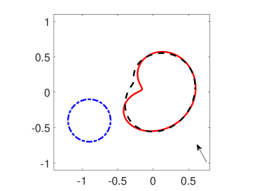
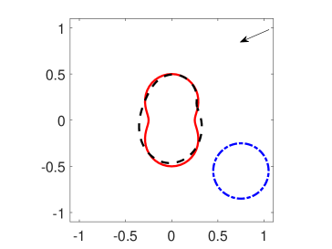
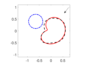
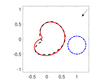
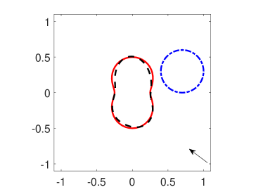
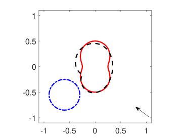
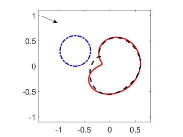
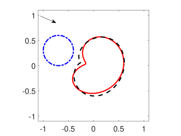
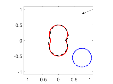
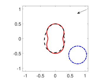
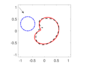
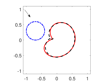
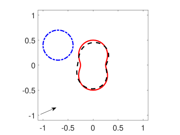
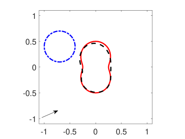
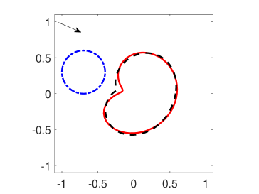
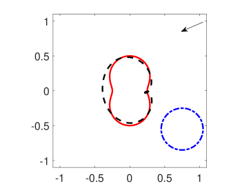
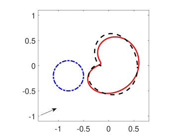
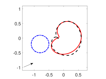
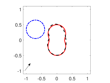
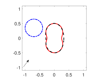
In all of the following figures, the exact boundary curves are displayed in solid lines, the reconstructed boundary curves are depicted in dashed lines $--$, and all the initial guesses are taken to be a circle with radius $r^{(0)}=0.3$ which is indicated in the dash-dotted lines $\cdot-$. The incident directions are denoted by directed line segments with arrows. Throughout all the numerical examples, we take $\lambda=3.88,\mu=2.56$, the scaling factor $\rho=0.9$, and the truncation $M=6$. The number of quadrature points is equal to 128, i.e., $n=64$. In addition, we choose the angular frequency $\omega=0.7\pi$ in Example 1 and $\omega=0.6\pi$ in Example 2 and Example 3. We present the results for two commonly used examples: an apple-shaped obstacle and a peanut-shaped obstacle. The parametrization of the exact boundary curves for these two obstacles are given in Table 1.

6.1. Example 1: the Phased IOSP

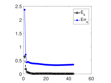
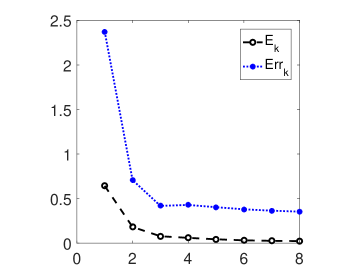
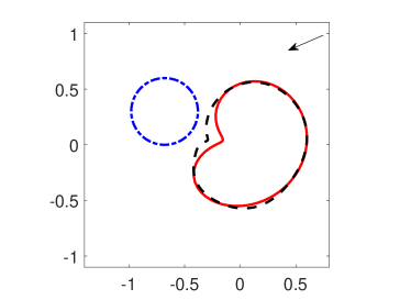
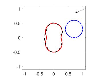
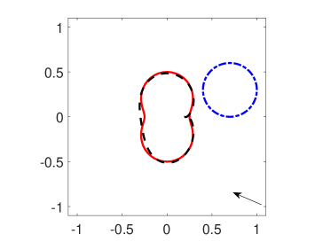
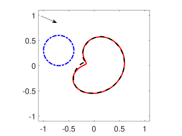
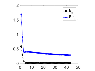
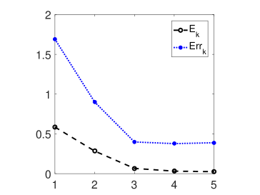
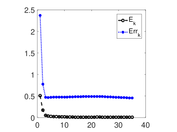
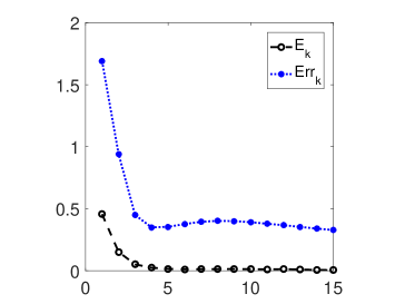
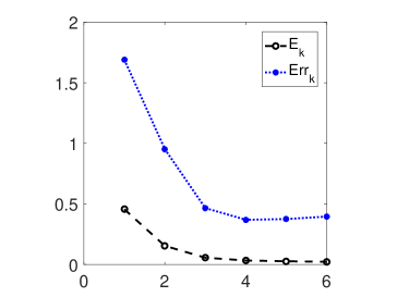
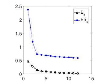
We consider an inverse elastic scattering problem of reconstructing a rigid obstacle from the phased far-field data by using Algorithm I. In Figures 2 and 3, the results are shown for the apple-shaped obstacle and the peanut-shaped obstacles with $1\%$ and $5\%$ noise, respectively. The relative $L^{2}$ error ${\rm Err}_{k}$ between the reconstructed obstacle and the exact obstacle and the relative error estimator ${\rm E}_{k}$ defined in (5.9) are plotted against the number of iterations. As can be seen from the error curves, the relative error estimator ${\rm E}_{k}$ follows the actual relative error ${\rm Err}_{k}$ very well and is a reasonable choice of the stopping criteria for the iterations. For the fixed incident direction, Figures 4 and 5 show the reconstructions of the apple-shaped obstacle and the peanut-shaped obstacle by using different initial guesses; for the fixed initial guess, Figures 6 and 7 show the reconstructions of the apple-shaped obstacle and the peanut-shaped obstacle by using different incident directions. As shown in these results, the reconstruction is not sensitive to the initial guess or the incident direction. The location and shape of the obstacle can be simultaneously and satisfactorily reconstructed for a single incident plane wave.

6.2. Example 2: the phased IOSP with a reference ball

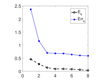
Now we investigate the inverse scattering problem of reconstructing a rigid obstacle from the phased far-field data by introducing a reference ball. The reconstructions with $1\%$ noise and $5\%$ noise for the apple-shaped and peanut-shaped obstacles are shown in Figure 8 and Figure 9, respectively. The relative $L^{2}$ error ${\rm Err}_{k}$ and the relative error estimator ${\rm E}_{k}$ are also presented in the figures. Tests are also done by using different initial guesses and different incident directions. In addition, we test the influence by using reference balls with different radius and location. For the fixed initial guess and incident direction, Figures 10 and 11 show the reconstructions of the apple-shaped obstacle and the peanut-shaped obstacle by using different reference balls. The reconstructed obstacles agree very well with exact ones. As can be seen, the results by using the reference ball technique are comparable with those without the reference ball in Example 1. The method works very well to reconstruct the location and the shape.

6.3. Example 3: the phaseless IOSP with a reference ball

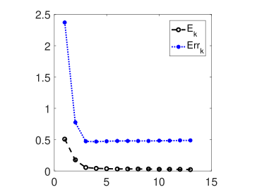
By adding a reference ball to the inverse scattering system, we consider the inverse scattering problem of reconstructing a rigid obstacle from phaseless far-field data by using Algorithm II. The reconstructions with $1\%$ noise and $5\%$ noise are shown in Figures 12–13. Again, the relative $L^{2}$ error ${\rm Err}_{k}$ and the relative error estimator ${\rm E}_{k}$ are plotted in the figures. Figures 14 and 15 show the reconstructions of the apple-shaped obstacle and the peanut-shaped obstacle by using different reference balls. From these figures, we observe that the translation invariance property of the phaseless far-field pattern can be broken by introducing a reference ball. Based on this technique, both of the location and shape of the obstacle can be satisfactorily reconstructed from the phaseless far-field data by using a single incident plane wave.

7. Conclusions and future works

In this paper, we have studied the two-dimensional inverse elastic scattering problem by the phased and phaseless far-field data for a single incident plane wave. Based on the Helmholtz decomposition, the elastic wave equation is reformulated into a coupled boundary value problem of the Hemholtz equation. The relationship between compressional or shear far-field pattern for the Navier equation and the corresponding far-field pattern for the Helmholtz equation are investigated. The translation invariance property of the phaseless compressional and shear far-field pattern is proved. A nonlinear integral equation method is developed for the inverse problem. For the phaseless data, we introduce a reference ball technique to the inverse scattering system in order to break the translation invariance. Numerical examples are presented to demonstrate the effectiveness and stability of the proposed method. Future work includes the different boundary conditions of the obstacle and the three-dimensional problem. It is a challenging problem for the uniqueness of the phaseless inverse elastic scattering problem with a reference ball. We intend to investigate these issues and report the progress elsewhere.

References

- [1] H. Ammari, E. Bretin, J. Garnier, H. Kang, H. Lee, and A. Wahab, Mathematical Methods in Elasticity Imaging, Princeton University Press, New Jersey, 2015.
- [2] H. Ammari, Y. T. Tin, and J. Zou, Phased and phaseless domain reconstruction in inverse scattering problem via scattering coefficients, SIAM J. Appl. Math., 76 (2016), pp. 1000–1030.
- [3] G. Bao and L. Zhang, Shape reconstruction of the multi-scale rough surface from multi-frequency phaseless data, Inverse Problems, 32 (2016), 085002.
- [4] G. Bao, P. Li, and J. Lv, Numerical solution of an inverse diffraction grating problem from phaseless data, J. Opt. Soc. Am. A, 30 (2013), pp. 293–299.
- [5] M. Bonnet and A. Constantinescu, Inverse problems in elasticity, Inverse Problems, 21 (2005), pp. 1–50
- [6] Z. Chen and G. Huang, A direct imaging method for electromagnetic scattering data without phase information, SIAM J. Imaging Sci., 9 (2016), pp. 1273–1297.
- [7] D. Colton and R. Kress, Inverse Acoustic and Electromagnetic Scattering Theory, 3rd edition, Springer, New York, 2013.
- [8] H. Dong, D. Zhang, and Y. Guo, A reference ball based iterative algorithm for imaging acoustic obstacle from phaseless far-field data, Inverse Probl. Imaging, accepted.
- [9] J. Elschner and M. Yamamoto, Uniqueness in inverse elastic scattering with finitely many incident waves, Inverse Problems, 26 (2010), 045005.
- [10] P. Gao, H. Dong, and F. Ma, Inverse scattering via nonlinear integral equations method for a sound-soft crack from phaseless data,Applications of Mathematics, 63 (2018), pp. 149–165.
- [11] P. Hahner and G. C. Hsiao, Uniqueness theorems in inverse obstacle scattering of elastic waves, Inverse Problems, 9 (1993), pp. 525–534.
- [12] G. Hu. A. Kirsch, and M. Sini, Some inverse problems arising from elastic scattering by rigid obstacles, Inverse Problems, 29 (2013), 015009
- [13] G. Hu, J. Li, H. Liu, and H. Sun, Inverse elastic scattering for multiscale rigid bodies with a single far-field pattern, SIAM J. Imaging Sci., 7 (2014), pp. 1799–1825.
- [14] O. Ivanyshyn, Shape reconstruction of acoustic obstacles from the modulus of the far field pattern, Inverse Probl. Imaging, 1 (2007), pp. 609–622.
- [15] O. Ivanyshyn and R. Kress, Identification of sound-soft 3D obstacles from phaseless data, Inverse Probl. Imaging, 4 (2010), pp. 131–149.
- [16] T. Johansson and B. D. Sleeman, Reconstruction of an acoustically sound-soft obstacle from one incident field and the far-field pattern, IMA J. Appl. Math., 72 (2007), pp. 96–112.
- [17] M. Kar and M. Sini, On the inverse elastic scattering by interfaces using one type of scattered waves, J. Elast., 118 (2015), pp. 15–38.
- [18] A. Karageorghis, B.T. Johansson, and D. Lesnic, The method of fundamental solutions for the identification of a sound-soft obstacle in inverse acoustic scattering, Appl. Numer. Math., 62 (2012), pp. 1767–1780.
- [19] M. V. Klibanov, Phaseless inverse scattering problems in three dimensions, SIAM J. Appl. Math., 74 (2014), pp. 392–410.
- [20] M. V. Klibanov, D. Nguyen, and L. Nguyen, A coefficient inverse problem with a single measurement of phaseless scattering data, preprint, 2017, arXiv:1710.04804v1.
- [21] R. Kress, On the numerical solution of a hypersingular integral equation in scattering theory, J. Comput. Appl. Math., 61 (1995), pp. 345–360.
- [22] R. Kress, Inverse elastic scattering from a crack, Inverse Problems, 12 (1996), pp. 667–684.
- [23] R. Kress, Newton’s method for inverse obstacle scattering meets the method of least squares, Inverse Problem, 19 (2003), pp. S91–S104.
- [24] R. Kress, Linear Integral Equations, 3rd edition, Springer, New York, 2014.
- [25] R. Kress and W. Rundell, Inverse obstacle scattering with modulus of the far field pattern as data, Inverse Problems in Medical Imaging and Nondestructive Testing, 1997, pp. 75–92.
- [26] J. Lai and P. Li, A fast solver for the elastic scattering by multi-particles, preprint.
- [27] L. D. Landau and E. M. Lifshitz, Theory of Elasticity, Oxford: Pergamon 1986.
- [28] F. Le Louër, A domain derivative-based method for solving elastodynamic inverse obstacle scattering problems, Inverse Problems, 31 (2015), 115006.
- [29] F. Le Louër, On the Fréchet derivative in elastic obstacle scattering, SIAM J. Appl. Math., 72 (2012), pp. 1493–1507.
- [30] K. M. Lee, Shape reconstructions from phaseless data, Eng. Anal. Bound. Elem., 71 (2016), pp. 174–178.
- [31] J. Li, H. Liu, and Y. Wang, Recovering an electromagnetic obstacle by a few phaseless backscattering measurements, Inverse Problems, 33 (2017), 035011.
- [32] J. Li, H. Liu, and J. Zou, Strengthened linear sampling method with a reference ball, SIAM J. Sci. Comput., 31 (2009), pp. 4013–4040.
- [33] P. Li, Y. Wang, Z. Wang, and Y. Zhao, Inverse obstacle scattering for elastic waves, Inverse Problems, 32 (2016), 115018.
- [34] P. Li, Y. Wang, and Y. Zhao, Inverse elastic surface scattering with near-field data, Inverse Problems, 31 (2015), 035009.
- [35] X. Liu and B. Zhang, Unique determination of a sound-soft ball by the modulus of a single far field datum, J. Math. Anal. Appl., 365 (2010), pp. 619–624.
- [36] X. Ji, X. Liu, and B. Zhang, Target reconstruction with a reference point scatterer using phaseless far field patterns, preprint, 2018, arXiv:1805.08035v3.
- [37] G. Nakamura and G. Uhlmann, Inverse problems at the boundary of elastic medium, SIAM J. Math. Anal., 26 (1995), pp. 263–279.
- [38] X. Xu, B. Zhang, and H. Zhang, Uniqueness in inverse scattering problems with phaseless far-field data at a fixed frequency, SIAM J. Appl. Math., 78 (2018), pp. 1737–1753.
- [39] J. Yue, M. Li, P. Li, and X. Yuan, Numerical solution of an inverse obstacle scattering problem for elastic waves via the Helmholtz decomposition, Commun. Comput. Phys., to appear.
- [40] D. Zhang and Y. Guo, Uniqueness results on phaseless inverse scattering with a reference ball, Inverse Problems, 34 (2018), 085002.
- [41] D. Zhang, Y. Guo, J. Li, and H. Liu, Retrieval of acoustic sources from multi-frequency phaseless data, Inverse Problems, 34 (2018), 094001.
- [42] B. Zhang and H. Zhang, Recovering scattering obstacles by multi-frequency phaseless far-field data, J. Comput. Phys., 345 (2017), pp. 58–73.
- [43] B. Zhang and H. Zhang, Fast imaging of scattering obstacles from phaseless far-field measurements at a fixed frequency, preprint, 2018, arXiv: 180509046v1.