Fixed points of mapping of N-point gravitational lenses

ABSTRACT. In this paper, we study fixed points of N-point gravitational lenses. We use complex form of lens mapping to study fixed points. Complex form has an advantage over coordinate one because we can describe N-point gravitational lens by system of two equation in coordinate form and we can describe it by one equation in complex form. We can easily transform the equation, which describe N-point gravitational lens, into polynomial equation that is convenient to use for our research. In our work, we present lens mapping as a linear combination of two mapping: complex analytical and identity mapping. Analytical mapping is specified by analytical function (deflection function). We studied necessary and sufficient conditions for the existence of deflection function and proved some theorems. Deflection function is analytical, rational, its zeroes are fixed points of lens mapping and their number is from 1 to N-1, poles of deflection function are coordinates of point masses, all poles are simple, the residues at the poles are equal to the value of point masses.
We used Gauss-Lucas theorem and proved that all fixed points of lens mapping are in the convex polygon. Vertices of the polygon consist of point masses. We proved theorem that can be used to find all fixed point of lens mapping. On the basis of the above, we conclude that one-point gravitational lens has no fixed points, 2-point lens has only 1 fixed point, 3-point lens has 1 or 2 fixed points. Also we present expressions to calculate fixed points in 2-point and 3-point gravitational lenses. We present some examples of parametrization of point masses and distribution of fixed points for this parametrization.
Keywords: gravitational lensing: lens mapping, fixed points, deflection function; complex analysis.

1. Introduction
Gravitational lensing is a phenomenon of deflection of light ray in a gravity field (Bliokh&Minakov,1989; Zakharov,1997;Schneider,1999). With gravitational lensing, star systems and planets in star systems can be found. Recently, astronomers have observed a large number of gravitational lenses. In addition to one-point lenses, lenses with more than two components were also detected. In this paper, we show that such objects can have fixed points. In physical terms, fixed point of gravitational lens is a point in a picture plane that has such property: if we place source in fixed point, one of images is in this point.
2. General information and formulation of the problem
An N-point gravitational lens can be described by means of the following equation (Zakharov,1997;Schneider,1999):

$$\vec{y}=\vec{x}-\sum_{n}m_{n}\frac{\vec{x}-\vec{l}_{n}}{\left|\vec{x}-\vec{l}_{n}\right|^{2}},$$ (1)

where $m_{n}$ are dimensionless masses whose position in the plane of the lens is determined by the normalized radius-vectors $\vec{l}_{n}$. It is plain, that $\sum_{n}m_{n}=1$.

We denote the set of radius-vectors $\vec{l}_{n}$ as $\Lambda=\left\{l_{i}|i=1,2,...,N\right\}$. Vector equation (1) specifies single-valued mapping

$$L:\left(R_{X}^{2}\backslash\Lambda\right)\rightarrow R_{Y}^{2},$$ (2)

from vector space $R_{X}^{2}$ to vector space $R_{Y}^{2}$.

We introduce Cartesian coordinates, that transforms $R_{X}^{2}$ and $R_{Y}^{2}$ spaces into coordinate planes. Coordinate planes $R_{Y}^{2}$ and $R_{X}^{2}$ are source plane and image plane respectively. Source plane $R_{Y}^{2}$ and image plane $R_{X}^{2}$ are often united and called picture plane in astrophysical literature.

Mapping (2) can be described by system of equations:

$$\left\{\begin{array}[c]{c}y_{1}=(x_{1}-\sum\limits_{n=1}^{N}m_{i}\frac{x_{1}-a_{n}}{\left(x_{1}-a_{n}\right)^{2}+\left(x_{2}-b_{n}\right)^{2}})\\ y_{2}=(x_{2}-\sum\limits_{n=1}^{N}m_{i}\frac{x_{2}-b_{n}}{\left(x_{1}-a_{n}\right)^{2}+\left(x_{2}-b_{n}\right)^{2}})\end{array}\right.,$$ (3)

where $\left(a_{n},b_{n}\right)$ are coordinates of point $C_{n}$ of radius-vector $\vec{l}_{n}$ in plane $R_{X}^{2}$.

Analytical research of (3) was in (Kotvytskiy&Bronza&Vovk, 2016; Bronza&Kotvytskiy, 2017; Kotvytskiy&Bronza&Shablenko, 2017), and quasianalytical method of image construction was offered in (Kotvytskiy&Bronza, 2016).

A point of single-valued mapping $L$ is fixed, if each of point coordinates is invariant of $L$.

We need to substitute $y_{1}=x_{1}$ and $y_{2}=x_{2}$ and into system of equations (3) and solve it to find fixed points.

$$\left\{\begin{array}[c]{c}\sum\limits_{n=1}^{N}m_{i}\frac{x_{1}-a_{n}}{\left(x_{1}-a_{n}\right)^{2}+\left(x_{2}-b_{n}\right)^{2}}=0\\ \sum\limits_{n=1}^{N}m_{i}\frac{x_{2}-b_{n}}{\left(x_{1}-a_{n}\right)^{2}+\left(x_{2}-b_{n}\right)^{2}}=0\end{array}\right.$$ (4)

Mapping $L$ is surjective. Inverse mapping

$$L^{-1}:R_{Y}^{2}\rightarrow\left(R_{X}^{2}\backslash\Lambda\right),$$ (5)

is multivalued. If $A_{0}$ - is a fixed point of single-valued mapping $L$, then image of its image, when the mapping is reversed, is not coincide with it, but includes it.

$$A_{0}\in L^{-1}\left(L\left(A_{0}\right)\right).$$ (6)

In this paper we study the set $\Xi$ of fixed points of mapping $L$.

We set the mapping $L$ in complex form for effective application of mathematical tool.
3. Complexification of lens mapping $L$
Let define mapping (3) in complex form. We introduce complex structure for $R_{X}^{2}$ and $R_{Y}^{2}$ , that transforms them into complex planes $\mathbb{C}_{z}$ and $\mathbb{C}_{\zeta}$ respectively.

We introduce new complex variables $z$ and $\zeta$ . Let

$$\operatorname{Re}z=x_{1},\operatorname{Im}z=x_{2},\operatorname{Re}\zeta=y_{1},\operatorname{Im}\zeta=y_{2}.$$ (7)

New variables related to old ones as

$$\left\{\begin{array}[c]{c}x_{1}=\frac{z+\overline{z}}{2}\\ x_{2}=\frac{z-\overline{z}}{2}\end{array}\right.and\left\{\begin{array}[c]{c}y_{1}=\frac{\zeta+\overline{\zeta}}{2}\\ y_{2}=\frac{\zeta-\overline{\zeta}}{2}\end{array}\right.,$$ (8)

Now system (3) can be written as

$$\zeta=z-\sum_{n=1}^{N}m_{n}\frac{1}{\overline{z}-\overline{A_{n}}},$$ (9)

where $\sum_{n=1}^{N}m_{n}=1$ and $A_{n}=a_{n}+ib_{n}$; $n=1,2,...,N$.

We introduce function $\omega=\sum_{n=1}^{N}m_{n}\frac{1}{\overline{z}-\overline{A_{n}}}$ and call it deflection function. Function is complex conjugated to $\omega$ and defined:

$$w=\sum_{n=1}^{N}m_{n}\frac{1}{z-A_{n}}$$ (10)

Functions $\omega$ and $w$ contain all the information about N-point gravitational lens. Except that it is convenient to use function $w$, rather than $\omega$, for application of methods of geometric function theory.

We have:

$$\zeta=z-\overline{w}\left(\overline{z}\right)=z-\overline{w\left(z\right)}.$$ (11)

Or:

$$\overline{\zeta}=\overline{z}-w\left(z\right).$$ (12)

Thus, N-point lens can be described not only by the system of equation (3) but also by the single equation (9). Mapping (2) can be written as

$$L:\left(\mathbb{C}_{X}\backslash\Lambda\right)\rightarrow\mathbb{C}_{Y},$$ (13)

mapping of complex plane $\mathbb{C}_{X}$ into complex plane $\mathbb{C}_{Y}$.

We can obtain equation (12) in another way. We can use equation (1) (Witt, 1990).
4. Some properties of $\zeta=\zeta\left(z\right)$ and $w=w\left(z\right).$

Statement 4.1. Function $\zeta=\zeta\left(z\right)$ is not an analytic function.

Proof. Derivative of $\zeta=\zeta\left(z\right)$

$$\frac{\partial\zeta}{\partial\overline{z}}=\frac{\partial}{\partial\overline{z}}\left(z-\overline{w}\left(\overline{z}\right)\right)=1-\frac{\partial\overline{w}}{\partial\overline{z}}\neq 0$$

is not identity equal zero, therefore $\zeta$ is not analytic function.

Statement 4.2. Deflection function $w=w\left(z\right)$ is an analytic function.

Proof. Derivative of $w=w\left(z\right)$

$$\frac{\partial w}{\partial\overline{z}}=\frac{\partial}{\partial\overline{z}}\left(\sum_{n=1}^{N}m_{n}\frac{1}{z-A_{n}}\right)=\sum_{n=1}^{N}m_{n}\frac{\partial}{\partial\overline{z}}\frac{1}{z-A_{n}}\equiv 0$$

is identity equal zero, therefore $w$ in an analytic function.

Statement 4.3. Deflection function $w=w\left(z\right)$ is:

• rational function, i.e. $w=\frac{A\left(z\right)}{B\left(z\right)},$ where $A\left(z\right)$ and $B\left(z\right)$ are polynomials;

• the denominator is a degree $\deg B\left(z\right)=N$, the numerator is a degree $\deg A\left(z\right)=N-1$;

• leading coefficients of $A\left(z\right)$ and $B\left(z\right)$ are equal 1.

Proof. We reduce the sum to common denominator

$$w=\sum_{n=1}^{N}m_{n}\frac{1}{z-A_{n}}.$$ (14)

Denominator of deflection function $B\left(z\right)=\prod\nolimits_{n=1}^{N}\left(z-A_{n}\right)$ is a degree $\deg B\left(z\right)=N$ leading coefficient equals 1. Numerator $A\left(z\right)=\sum_{n=1}^{N}m_{n}z^{N-1}+...$ is a degree $\deg A\left(z\right)=N-1$, leading coefficient of $A\left(z\right)$ equals $\sum_{n=1}^{N}m_{n}=1.$

Theorem 4.4. Deflection function $w$ can be written in form:

$$a)w=\frac{Q^{\prime}\left(z\right)}{Q\left(z\right)},$$ (15)

where $Q\left(z\right)=\prod\nolimits_{n=1}^{N}\left(z-A_{n}\right)^{m_{n}}$;

$$b)w=\frac{1}{\deg P\left(z\right)}\frac{P^{\prime}\left(z\right)}{P\left(z\right)},$$ (16)

where $P\left(z\right)$ is polynomial;

Proof. a) $w=\sum\limits_{n=1}^{N}m_{n}\frac{1}{z-A_{n}}=\\ =\sum\limits_{n=1}^{N}\left(m_{n}\frac{d}{dz}\left(\ln\left(z-A_{n}\right)\right)\right)=\\ =\sum\limits_{n=1}^{N}\frac{d}{dz}\left(\ln\left(z-A_{n}\right)^{m_{n}}\right)=\\ =\frac{d}{dz}\left(\ln\left(\prod\limits_{n=1}^{N}\left(z-A_{n}\right)^{m_{n}}\right)\right)=\frac{d}{dz}\left(\ln Q\left(z\right)\right)=\frac{Q^{\prime}\left(z\right)}{Q\left(z\right)}.$

We note, that function $Q\left(z\right)$ is not a polynomial.

Proof. b)$w=\frac{Q^{\prime}\left(z\right)}{Q\left(z\right)}=\frac{d}{dz}\left(\ln Q\left(z\right)\right)=\\ =\frac{d}{dz}\left(\ln\left(\prod\nolimits_{n=1}^{N}\left(z-A_{n}\right)^{m_{n}}\right)\right).$

Assume without loss of generality, that numbers $m_{n}$ are rational.

Let $m_{n}=\frac{p_{n}}{q_{n}}$, where $p_{n}$ and $q_{n}$ are natural numbers and coprime integers.

We substitute that into equation and transform it. Whence, we have:

$$w=\frac{d}{dz}\left(\frac{1}{h}\ln\left(\prod\nolimits_{n=1}^{N}\left(z-A_{n}\right)^{\frac{p_{n}}{q_{n}}h}\right)\right),$$ (17)

where $h=\prod\nolimits_{n=1}^{N}q_{n}$. Let $s_{n}=\frac{p_{n}}{q_{n}}h$. Numbers $s_{n}$ are natural numbers.

After transformation (17) we have:

$$w=\frac{d}{dz}\left(\frac{1}{h}\ln{P}\left(z\right)\right)=\frac{d}{dz}\left(\frac{1}{h}P\left(z\right)\right)=\frac{1}{h}\frac{P^{\prime}}{P},$$ (18)

where $P\left(z\right)=\prod\limits_{n=1}^{N}\left(z-A_{n}\right)^{s_{n}}$ is polynomial. But then

$$w=\frac{1}{h}\frac{1}{h}\frac{P^{\prime}\left(z\right)}{P\left(z\right)}.$$ (19)

As well, leading coefficients of $A\left(z\right)$ and $B\left(z\right)$ are equal 1 and leading coefficient of $P^{\prime}\left(z\right)$ equal $\deg P\left(z\right)$. We have: $h=\deg P\left(z\right)$, i.e. we have (16). QED.

Remark 1 (to theorem 4.4). Polynomials $P\left(z\right)$ and $P^{\prime}\left(z\right)$ have the same roots as $B\left(z\right)=\prod\limits_{n=1}^{N}\left(z-A_{n}\right)$, but with different multiplicity.

Remark 2 (to theorem 4.4). Then since function $\omega$ is complex conjugate to $w$, we obviously have:

$$\omega =\overline{w}=\overline{\left(\frac{1}{h}\frac{P^{\prime}\left(z\right)}{P\left(z\right)}\right)}=\frac{1}{h}\frac{\overline{P\left(z\right)}}{\overline{P\left(z\right)}}=$$ (20)

$$=\frac{1}{h}\frac{\left(\overline{P\left(z\right)}\right)^{\prime}}{\overline{P\left(z\right)}}=\frac{1}{h}\frac{\overline{P}^{\prime}\left(\overline{z}\right)}{\overline{P}\left(\overline{z}\right)}.$$

Function $\omega$, exactly as $w$, can be expressed in form of ratio of two polynomials. Numerator of the ratio is a derivative of denominator up to an unessential constant multiplier.

Remark 3 (to theorem 4.4). Polynomials $P\left(z\right)$ and $P^{\prime}\left(z\right)$ are not coprime. Fraction $\frac{P^{\prime}\left(z\right)}{P\left(z\right)}$ can be reduced. Polynomials $P\left(z\right)$ and $P^{\prime}\left(z\right)$ are coprime, if and only if $m_{n}=\frac{1}{N},n=1,2,...,N$.

Theorem 4.6. Poles of function $w$ are $A_{n}$ points, which are coordinates of masses. All poles are simple. For any poles are always true: pole residue equal normalized mass at that point. The sum of residues at finite points into complex plane equal one. At infinity equal minus one. Proof. Obviously.
5. Fixed points of a lens mapping
Theorem 5.1.(About quantity) By $n_{0}$ denote a quantity of a fixed points of mapping $L:\left(\mathbb{C}_{X}\backslash\Lambda\right)\rightarrow\mathbb{C}_{Y}$, then $n_{0}:1\leq n_{0}\leq N-1$.

Proof. Fixed points of function $\zeta=z-\overline{w}\left(\overline{z}\right)$ are roots of equation $z=z-\overline{w}\left(\overline{z}\right)$, i.e. $\overline{w}\left(\overline{z}\right)=0$. We have $w\left(z\right)=0$, if we complex conjugate it.

Therefore, we have $\deg P^{\prime}\left(z\right)=N-1$ from the representation (16). Hence, the number of zeroes of function $w$ with regard to multiplicity is $N-1$. Polynomial $P^{\prime}\left(z\right)$ can have multiple zeroes. The number of different zeroes of polynomial $P^{\prime}\left(z\right)$ is from $1$ to $N-1$.

We have the theorem about distribution of a fixed points of mapping $L$.

Theorem (main) 5.2. (About distribution) Fixed points of mapping $L$ are in the convex polygon that consists of point masses.

Proof. We use Gauss-Lucas theorem: if $P$ is a polynomial with complex coefficients, all zeros of $P^{\prime}$ belong to the convex hull of the set of zeros of $P$.

By theorem 5.1, fixed points of mapping $L$ are zeroes of the function $w$. By theorem 4.5 we have representation (16).

Since $P\left(z\right)=\prod\limits_{n=1}^{N}\left(z-A_{n}\right)^{s_{n}}$, roots of $P^{\prime}\left(z\right)$,are in the convex polygon that consists of set $\left\{A_{n}\right\}$, because of Gauss-Lucas theorem (Prasolov,2014;Davydov,1964).

Theorem 5.3. (of finding fixed points and its number) Fixed points of mapping $L$ for $N\geq 2$ are roots of:

$$H\left(z\right)=\frac{P\left(z\right)}{\gcd\left(P\left(z\right),P^{\prime}\left(z\right)\right)},$$ (21)

their number $n_{0}=\deg H\left(z\right),$ and estimation $n_{0}:1\leq n_{0}\leq N-1$ is achieved.

Proof. The polynomial $P\left(z\right)$ is divided by the polynomial $\gcd\left(P\left(z\right),P^{\prime}\left(z\right)\right)$. Therefore $B\left(z\right)$ is a polynomial. Polynomial $\gcd\left(P\left(z\right),P^{\prime}\left(z\right)\right)$ has only multiple roots. Multiplicity of roots of $\gcd\left(P\left(z\right),P^{\prime}\left(z\right)\right)$ is one less then multiplicity of $P\left(z\right)$. Hence all roots of polynomial $H\left(z\right)$ are different and $n_{0}=\deg H\left(z\right)$.

2-point gravitational lens has one fixed point.

In general situation the number of fixed points is $n_{0}=N-1$.

For $N>2$, we have only one fixed point, if and only if all point masses are equal and located at the vortexes of regular polygon.

Remark 4 (to theorem 5.3). Fixed points are missing from point gravitational lens.
6. Examples
For 1-point lens we have deflection function

$$w=\sum\limits_{n=1}^{N}\frac{m_{n}}{z-A_{n}}=\frac{m_{1}}{z-A_{1}},$$

where $m_{1}=1$ and $A_{1}=0$.

For 2-point lens we have deflection function

$$w=\frac{m_{1}}{z-A_{1}}+\frac{m_{2}}{z-A_{2}}$$

where $A_{1}$ and $A_{2}$ are coordinates of point masses and $m_{1}+m_{2}=1$.

With $m_{1}=s,m_{2}=1-s$ and $s\in\left[0,1\right]$ we have

$$z_{st} =A_{1}+\left(A_{2}-A_{1}\right)s$$

For 3-point lens we have deflection function

$$w=\frac{m_{1}}{z-A_{1}}+\frac{m_{2}}{z-A_{2}}+\frac{m_{3}}{z-A_{3}}$$

where $A_{1},A_{2},A_{3}$ are coordinates of point masses and $m_{1}+m_{2}+m_{3}=1$.

We have an equation for fixed points

$$z^{2}+A_{2}A_{3}m_{1}+A_{1}A_{3}m_{2}+A_{1}A_{2}m_{3}-$$

$$-\left(A_{2}m_{1}+A_{3}m_{1}+A_{1}m_{2}+A_{3}m_{2}+A_{1}m_{3}+A_{2}m_{3}\right)z=0$$

Figure 1: 3-point lens with $m_{1}=1-s,m_{2}=\frac{s}{2},m_{3}=\frac{s}{2},A_{1}=1,A_{2}=i,A_{3}=-i$

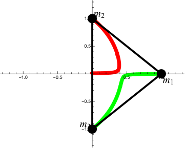
Figure 2: 3-point lens with $m_{1}=1-s,m_{2}=0.495s,m_{3}=0.505s,A_{1}=1,A_{2}=i,A_{3}=-i$

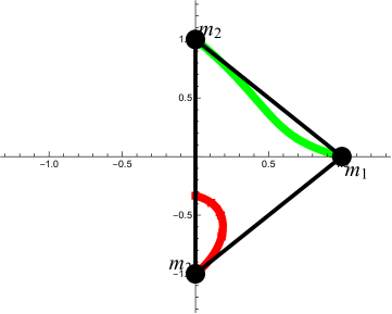
Figure 3: 3-point lens with $m_{1}=1-s,m_{2}=\frac{2s}{3},m_{3}=\frac{s}{3},A_{1}=1,A_{2}=i,A_{3}=-i$

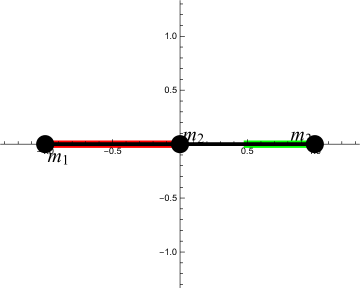
Figure 4: 3-point lens with $m_{1}=1-s,m_{2}=\frac{s}{2},m_{3}=\frac{s}{2},A_{1}=-1,A_{2}=0,A_{3}=1$

Acknowledgements. Albert Kotvytskiy and Volodymyr Shablenko thank for support SFFR, Ukraine, Project No. 32367.
References
Bliokh P.V., Minakov A.A.: 1989, Gravitational Lenses [in Russian]. (Naukova Dumka, Kiev), 240
Zakharov A.F.: 1997, Gravitacionnye linzy i mikrolinzy [in Russian]. (Janus-K, Moskow), 328
Schneider P., Ehlers J., Falco E.E.: 1999, Gravitational Lenses. (Springer-Verlag Berlin Heidelberg), 560
Kotvytskiy A.T., Bronza S.D., Vovk S.R.: 2016, Bulletin of Kharkiv Karazin National University “Physics”, 24, 55 (arXiv:1809.05392)
Bronza S.D., Kotvytskiy A.T.: 2017, Bulletin of Kharkiv Karazin National University “Physics”, 26, 6
Kotvytskiy A.T., Bronza S.D., Shablenko V.Yu.: 2017, Odessa Astronomical Publications, 30, 35
Kotvytskiy A.T., Bronza S.D.: 2016, Odessa Astronomical Publications, 29, 31
Witt H.J.: 1990, A&A, 236,311
Praslov V.V.:2014, Polynomials[in Russian]. MCCME, 336
Davydov N.A.:1964, USSR Computational Mathematics and Mathematical Physics, 4,No.2, 257