BioSimulator.jl: Stochastic simulation in Julia

$\ast$ Corresponding author at:
Division of Hematology-Oncology
Department of Medicine
100 UCLA Medical Plaza, Suite 550, Los Angeles, CA 90095–7059, USA
Tel.: +1/310/825–9203
Fax: +1/310/443–0477

E-mail addresses: alanderos@ucla.edu (A. Landeros), stutztim@ucla.edu (T. Stutz), klkeys@g.ucla.edu (K. L. Keys), alekseye@musc.edu (A. Alekseyenko), JanetS@mednet.ucla.edu (J. S. Sinsheimer), klange@ucla.edu (K. Lange), msehl@mednet.ucla.edu (M. E. Sehl)

Abstract

Background and Objectives: Biological systems with intertwined feedback loops pose a challenge to mathematical modeling efforts. Moreover, rare events, such as mutation and extinction, complicate system dynamics. Stochastic simulation algorithms are useful in generating time-evolution trajectories for these systems because they can adequately capture the influence of random fluctuations and quantify rare events. We present a simple and flexible package, BioSimulator.jl, for implementing the Gillespie algorithm, $\tau$-leaping, and related stochastic simulation algorithms. The objective of this work is to provide scientists across domains with fast, user-friendly simulation tools.

Methods: We used the high-performance programming language Julia because of its emphasis on scientific computing. Our software package implements a suite of stochastic simulation algorithms based on Markov chain theory. We provide the ability to (a) diagram Petri Nets describing interactions, (b) plot average trajectories and attached standard deviations of each participating species over time, and (c) generate frequency distributions of each species at a specified time.

Results: BioSimulator.jl’s interface allows users to build models programmatically within Julia. A model is then passed to the Conclusion: The user-friendly nature of BioSimulator.jl encourages the use of stochastic simulation, minimizes tedious programming efforts, and reduces errors during model specification. Keywords: stochastic simulation, Gillespie algorithm, $\tau$-leaping, systems biology, Julia language

1 Introduction

Biological systems with overlapping feedback and feedforward loops are often inherently stochastic. Furthermore, large, complex systems are mathematically intractable, and dynamical predictions based on deterministic models can be grossly misleading [29, 13]. Stochastic simulation algorithms based on continuous-time Markov chains allow researchers to generate accurate time-evolution trajectories, test the sensitivity of models to key parameters, and quantify frequencies of rare events [16, 35, 12, 34]. Stochastic simulation is helpful in cases where (a) rare events, such as extinction or mutation, influence system dynamics, (b) population compartments, such as numbers of biochemical molecules, are present in small numbers, and (c) population cycles arise from demographic stochasticity. Examples of such systems include gene expression networks, tumor suppressor pathways, and demographic and ecological systems. The current paper introduces a simple and flexible package, BioSimulator.jl, for implementing popular stochastic simulation algorithms based on Markov chain theory. BioSimulator.jl builds on previous software. Notable examples include:

• StochSS, an integrated framework for deploying simulations on high-performance clusters [10]. It features a graphical interface for model editing, tools for deterministic, stochastic, and spatial simulations, a model analysis toolkit, and data visualization. StochKit2, a mature C++ library of stochastic simulation algorithms, serves as the simulation engine.

• StochPy, an interactive stochastic modeling tool written in Python [27]. It provides a number of simulation algorithms, including delayed and single molecule methods.

• GillespieSSA, an R implementation of exact and approximate simulation algorithms [30]. Gillespie.jl is a Julia extension of the original R package [14]. Today, Gillespie.jl features Jensen’s uniformization method and the True Jump Method.

• DifferentialEquations.jl, an extensive Julia ecosystem for solving differential equations [31].

In addition, there are many specialized biological modeling tools:

• COPASI, a large open-source software application for analyzing and simulating biochemical networks models [24]. It features a user-friendly graphical interface and supports both differential equation modeling and stochastic simulation algorithms.

• Smoldyn, a particle-based stochastic spatial simulation engine [1]. It emphasizes biophysical and cell environment modeling.

• BioNetGen, a rules-based model editor and simulation framework that focuses on cell regulatory networks [22].

• PySB, a Python module for building mathematical descriptions of biological networks [26]. It provides a domain-specific language that is translated into a portable intermediate model representation. PySB connects to other software tools, such as SciPy and StochKit2, for simulations.

These packages have grown more sophisticated over time. Our goal in developing BioSimulator.jl is to provide a fast, open-source, and user-friendly library of stochastic simulation algorithms. BioSimulator.jl is written in the high-level, high-performance programming language Julia [2]. Our software consists of three main components: an interactive interface for model prototyping, a simulation engine, and a small library of stochastic simulation algorithms. We briefly review the theory underlying stochastic simulation in Section 2 and present the algorithms implemented by BioSimulator.jl in Section 3. Section 4 outlines the model development process and describes the available visualization tools. We summarize BioSimulator.jl’s graphical inputs and outputs, including (a) Petri nets describing the connectivity of the reaction network, (b) time-evolution trajectories of the system, and (c) frequency distributions of events. Three examples from biology, chemistry, and genetics in Section 5 illustrate how to define a model in BioSimulator.jl and simulate it as a continuous-time Markov chain. BioSimulator.jl will be valuable to a broad range of molecular and systems biologists, physicists, chemists, applied mathematicians, statisticians, and computer scientists interested in stochastic simulation modeling.

2 Background

2.1 Markov jump processes

Before we discuss simulation specifics, we describe the time evolution of a Markov jump process [25]. The underlying Markov chain follows a column vector $\mathbf{X}_{t}$ whose $i$-th component ${X}_{ti}$ is the number of particles of type $i$ at time $t\geq 0$. The components of $\mathbf{X}_{t}$ track species counts and are necessarily non-negative integers. The system starts at time $0$ and evolves via a succession of random reactions. Let $c$ denote the number of reaction channels and $d$ the number of particle types. Channel $j$ is characterized by a propensity function $r_{j}(\mathbf{x})$ depending on the current vector of counts $\mathbf{x}$. In a small time interval of length $s$, we expect $r_{j}(\mathbf{x})s+o(s)$ reactions of type $j$ to occur. Reaction $j$ changes the count vector by a fixed integer vector $\mathbf{v}^{j}$. Some components $v_{k}^{j}$ of $\mathbf{v}^{j}$ may be positive, some 0, and some negative. From the wait and jump perspective of Markov chain theory, the chain waits an exponential length of time until the next reaction. If the chain is currently in state $\mathbf{x}\equiv\mathbf{X}_{t}$, then the intensity of the waiting time until the next reaction is $r_{0}(\mathbf{x})=\sum_{j=1}^{c}r_{j}(\mathbf{x})$. Once the decision to jump is made, the chain jumps to the neighboring state $\mathbf{x}+\mathbf{v}^{j}$ with probability $r_{j}(\mathbf{x})/r_{0}(\mathbf{x})$. Table 1 lists typical reactions, their propensities $r(\mathbf{x})$, and increment vectors $\mathbf{v}$. In the table, $S_{i}$ denotes a single particle of type $i$. Only the nonzero increments $v_{i}$ are shown. The reaction propensities invoke the law of mass action and depend on rate constants $a_{i}$ [23]. Each discipline has its own vocabulary. Chemists use the term propensity instead of the term intensity and call the increment vector a stoichiometric vector. Physicists prefer creation to immigration. Biologists speak of death and mutation rather than of decay and isomerization.

Name	Reaction	$r(\mathbf{x})$	$\mathbf{v}$
Immigration	$0\to S_{1}$	$a_{1}$	$v_{1}=1$
Decay	$S_{1}\to 0$	$a_{2}x_{1}$	$v_{1}=-1$
Dimerization	$S_{1}+S_{1}\to S_{2}$	$a_{3}\binom{x_{1}}{2}$	$v_{1}=-2,v_{2}=1$
Isomerization	$S_{1}\to S_{2}$	$a_{4}x_{1}$	$v_{1}=-1,v_{2}=1$
Dissociation	$S_{2}\to S_{1}+S_{1}$	$a_{5}x_{2}$	$v_{1}=2,v_{2}=-1$
Budding	$S_{1}\to S_{1}+S_{2}$	$a_{6}x_{1}$	$v_{2}=1$
Replacement	$S_{1}+S_{2}\to S_{2}+S_{2}$	$a_{7}x_{1}x_{2}$	$v_{1}=-1,v_{2}=1$
Complex Reaction	$S_{1}+S_{2}\to S_{3}+S_{4}$	$a_{8}x_{1}x_{2}$	$v_{1}=v_{2}=-1,v_{3}=v_{4}=1$

Table 1: Propensities $r(\mathbf{x})$ and increment vectors $\mathbf{v}$ for some typical reactions. Here, $S_{i}$ denotes a single particle of type $i$, and $a_{i}$ denotes the reaction rate constant.

Often one is interested in the finite-time transition probabilities of a Markov chain. Let $p_{\mathbf{x},\mathbf{y}}(t)$ denote the probability that a Markov chain starting at state $\mathbf{x}$ transitions to state $\mathbf{y}$ by time $t$. The chemical master equation reads

$$p_{\mathbf{x},\mathbf{y}}(t+dt)=p_{\mathbf{x},\mathbf{y}}(t)\left[1-\sum_{j=1}^{c}a_{j}(\mathbf{y})dt\right]+\sum_{j=1}^{c}p_{\mathbf{x},\mathbf{y}-\mathbf{v}^{j}}(t)\ a_{j}(\mathbf{y}-\mathbf{v}^{j})dt+o(dt),$$

or equivalently, in differential form

$$\frac{d}{dt}p_{\mathbf{x},\mathbf{y}}(t)=\sum_{j=1}^{c}\left[p_{\mathbf{x},\mathbf{y}-\mathbf{v}^{j}}(t)\ a_{j}(\mathbf{y}-\mathbf{v}^{j})-p_{\mathbf{x},\mathbf{y}}(t)\ a_{j}(\mathbf{y})\right].$$

The differential form is a system of possibly infinitely-many coupled differential equations. Solving the master equation is an enormous endeavor except in the simplest of models. Alternatively, simulating multiple realizations of the process yields data that can then be used to estimate transition probabilities and summary statistics. References [16, 17] offer a first-principles derivation of the chemical master equation for biochemical reactions and connect this formalism to simulation methods.

2.2 The Julia language

Julia is a fast, expressive, and flexible programming language for scientific computing [2]. Specifically, the language targets the so-called two-language problem, in which a methods developer builds working prototypes in a slow high-level language only to then move performance-critical subroutines to a fast low-level language. The implicit assumption is that high-level, dynamic languages are expressive and therefore easier to use but at the expense of performance. For example, some language features, such as “for loops”, may incur performance penalties through no fault of the user. Such performance hurdles are overlooked because dynamic programming languages typically avoid tedious compilation steps and provide users with an intuitive syntax. High-level languages allow users to express the tasks they wish to complete by handling the low-level details. On the other hand, low-level languages typically require technical expertise and offer the fastest possible execution. A consequence of the two-language problem is that many tools, especially scientific software, become fragmented and difficult to manage. This is all the more relevant to scientists who often lack the necessary skills to maintain a software engineering project. Julia tackles this problem by providing an intuitive syntax and language features compatible with high performance underneath the hood, thereby making the user all the more productive. Interested readers are encouraged to peruse [2] for a deeper look into the Julia philosophy. Many online tutorials for learning Julia are available at https://julialang.org/learning/.

3 Simulation methods

BioSimulator.jl supports five different simulation algorithms. In the following subsections, we review each algorithm and briefly describe its strengths and weaknesses. The purpose of this section is to provide the reader with a high-level understanding of each algorithm and develop an intuition as to where methods succeed and fail. There are many references that provide details on these simulation methods, elucidate connections to spatial systems and related stochastic models, and motivate applications in many fields [20, 21].

3.1 Stochastic simulation algorithm

The Stochastic Simulation Algorithm (SSA), also known as the Direct or Gillespie method, implements the wait and jump mechanism for simulating a continuous-time Markov chain [16, 17]. At each step, the algorithm computes the propensities $r_{j}(\mathbf{x})$ of each reaction channel and generates two random deviates. One of these is an exponential deviate indicating the time to the next reaction based on $r_{0}(\mathbf{x})$. The second is a uniform random number $U(0,1)$ determining which reaction fires next based on the ratios $r_{j}(\mathbf{x})/r_{0}(\mathbf{x})$. The two main computational steps in the SSA are

1. Generate a random time $s$ to the next event by sampling from an exponential distribution with rate $r_{0}(\mathbf{x})$. This provides the update $t\mapsto t+s$.

2. Generate a random index $j$ denoting the reaction that occurred by sampling a categorical distribution with probabilities $r_{j}(\mathbf{x})/r_{0}(\mathbf{x})$. This provides the update $\mathbf{x}\mapsto\mathbf{x}+\mathbf{v}^{j}$.

Since the propensities $r_{j}(\mathbf{x})$ change after each event, the distributions underlying steps (I) and (II) change over time. Every Gillespie-like simulation algorithm is effectively distinguished by the sampling procedures used to generate the required random numbers, and the algorithms that update the underlying probability distributions. The main advantage of the SSA is its ability to produce statistically correct trajectories and distributions by simulating every reaction. This strength is also its greatest weakness in models where a small subset of frequently occurring reactions dominate simulation. The detailed computational analysis of Cao et al. identifies the linear search on the propensities $r_{j}(\mathbf{x})$ as a major obstacle to fast simulation [5]. The algorithm does not scale well with model size in the presence of different time scales. Thus, one must balance the value of accurate results versus speed in selecting SSA for simulation.

3.2 First reaction method

Gillespie proposed the First Reaction Method (FRM) as an alternative to SSA [16]. The main difference is the time to the next reaction

$$\tau=\underset{1\leq j\leq c}{\min}\{w_{1},\ldots,w_{c}\}$$

defined by independent exponentially distributed waiting times $w_{1},\ldots,w_{c}$ with intensity $r_{j}$. Here $c$ again denotes the total number of reaction channels. The premise of the algorithm is to compute the minimum of $c$ exponential random variables explicitly. This approach is less computationally efficient than SSA in the number of exponential deviates required to compute the time to the next event. We include the FRM in BioSimulator.jl purely for educational purposes. While the FRM does not offer any advantage over the original SSA, it provides a different way of thinking about simulation. The Next Reaction Method builds upon this idea.

3.3 Next reaction method

The Next Reaction Method (NRM), also known as the Gibson-Bruck method, is another exact algorithm equivalent to SSA [15]. At time $t=0$, the algorithm seeds each reaction channel $j$ a firing time $\tau_{j}$ and stores them inside a priority queue. In this context, a priority queue is a data structure that sorts pairs $(j,\tau_{j})$ according to the value of $\tau_{j}$ in increasing order. That is, if $\tau_{J}$ is the minimum time, then the pair $(J,\tau_{J})$ appears at the top of the queue. Thus, the next reaction is $J$ and its firing time is $\tau_{J}$; all other reactions fire at some future time. After reaction $J$ fires, the NRM updates the state vector $\mathbf{x}\to\mathbf{x}+\mathbf{v}^{J}$. The next firing time $\tau_{J}$ is also updated by an appropriate exponential deviate:

$$\tau_{J,\mathrm{new}}=\tau_{J,\mathrm{old}}+\mathrm{Exponential}(r_{J,\mathrm{new}}(\mathbf{x})),$$

where $r_{J,\mathrm{new}}(\mathbf{x})$ is the new propensity value. The remaining firing times change according to the recipe

$$\tau_{j,\mathrm{new}}=t+\frac{r_{j,\mathrm{old}}}{r_{j,\mathrm{new}}}(\tau_{j,\mathrm{old}}-t),\quad j\neq J,$$

based on the lack of memory property of the exponential distribution. The NRM also minimizes the number of propensities updated by tracking dependencies between reaction channels. Typically, the SSA sweeps through all the propensities $r_{j}(\mathbf{x})$ to reflect the change in $\mathbf{x}$. However, a reaction channel’s propensity only changes when the previous reaction event affected components of $\mathbf{x}$ that appears as reactants. The NRM uses a reaction dependency graph to describe these relationships between reactions. This data structure reduces the number of propensities that must be updated. Kahan summation can also be used to update the cumulative intensity $r_{0}(\mathbf{x})$ efficiently [15, 28]. The NRM excels in simulating systems with large numbers of species and lightly coupled reactions. Otherwise, in the extreme case, the algorithm must recalculate every firing time at every step. Systems with heavily coupled reaction channels are problematic for the NRM [5]. In this setting, the NRM becomes identical to the SSA but with the added burden of maintaining its priority queue.

3.4 Optimized direct method

The Optimized Direct Method (ODM) improves upon the original SSA by exploiting multi-scale properties inherent in large models [5]. BioSimulator.jl’s ODM implementation simulates a system once to count the number of times each reaction fires. This allows one to classify each reaction channel as fast (high frequency) or slow (low frequency). Sorting the reactions from fast to slow reduces the search depth in selecting the next reaction. This approach works well with heavily coupled reactions. Some systems exhibit more erratic behavior that prohibits classifying a reaction fast or slow. That is, switching between different time scales thwarts the ODM’s sorting optimization. The auto-regulation genetic network in Example 3 is an example of a system that undermines the optimized sorting of ODM.

3.5 $\tau$-leaping

BioSimulator.jl implements performance optimizations described by Mauch and Stalzer to improve SSA, FRM, NRM, and ODM techniques [28]. However, algorithms that simulate every reaction ultimately succumb to the high computational expense of large models. The $\tau$-leaping framework attempts to accelerate simulation by lumping reaction events together within a time leap $\tau$, selected to be as large as possible [18, 19, 7]. The basic $\tau$-leaping formula is

$$\mathbf{X}_{t+\tau}=\mathbf{X}_{t}+\sum_{j=1}^{c}\mathbf{v}^{j}Y_{j}(r_{j}(\mathbf{X}_{t})\tau).$$

where $Y_{j}$ is a Poisson random variable with rate $r_{j}(\mathbf{X}_{t})\tau$. Thus, $\tau$-leaping accelerates the SSA by lumping together multiple reaction events over an interval of size $\tau$. The main challenge in $\tau$-leaping is selecting the step size as large as possible while satisfying the leap condition

$$\left|r_{j}(\mathbf{X}_{t+\tau})-r_{j}(\mathbf{X}_{t})\right|\leq\epsilon,\quad j=1,2,\ldots,c,$$

which states that the propensity for each reaction $j$ is approximately constant over a leap of size $\tau$. Here, $\epsilon\in(0,1]$ is a prescribed acceptable change in propensities that controls the accuracy of sample paths generated by a $\tau$-leaping algorithm. A larger $\epsilon$ allows for larger leaps, while a smaller $\epsilon$ restricts leap size. In practice, many $\tau$-leaping algorithms employ a surrogate condition that satisfies the leap condition with high probability. In the stochastic simulation setting, a system is said to be stiff if the dynamics force a simulator to take “small” steps. Stiffness arises for a variety of reasons. Large models typically have a number of reactions occurring within a given interval. Reactions occurring on separate time scales split the system between “fast” and “slow” reactions, with the former occurring in a nearly deterministic fashion. In any case, stiffness causes the number of simulated events to increase in exact methods like the SSA. Stiffness poses a second threat to $\tau$-leaping methods. In addition to decreasing the leap size, stiffness can cause $\tau$-leaping to generate an excess of events due to the unbounded nature of the Poisson distribution. There are two precautionary measures to protect against aberrant behavior in $\tau$ selection [6, 33]. For example, a $\delta$ parameter controls whether $\tau$-leaping will default to SSA when the leap size is less than the expected change under the SSA; that is, if $\tau<\delta\cdot 1/r_{0}(\mathbf{x})$. This precaution is necessary to avoid taking suboptimal steps that introduce error and to mitigate leaps that send the system into negative population counts. In the event of a negative excursion, an acceptance parameter $\beta$ in $(0,1)$ contracts the leap step, effectively thinning the number of reaction events. Specifically, each event in a bad leap is randomly accepted if a uniform deviate $U(0,1)$ is less than $\beta$. The leap size $\tau$ is then set to $\tau\mapsto\beta\tau$. Leap contraction introduces bias in sample paths, so one must take care in setting $\beta$. As a rule of thumb, one should first select conservative values for $\epsilon$, $\beta$, and $\delta$ and test performance using short numerical experiments. BioSimulator.jl sets $\epsilon=0.03$, $\beta=0.75$, and $\delta=2$ as default values, drawn from the literature, that ought to perform well in many cases. $\tau$-leaping discards reaction event times but reduces the burden of random number generation. Each leap in the algorithm requires $c$ Poisson random deviates, one for each reaction channel. This accelerates simulation when the leap size $\tau$ is significantly large compared to a single SSA step. Like the SSA, there are many sophisticated variations on the original $\tau$-leaping algorithm. BioSimulator.jl implements the version found in [19] and is referred to as Ordinary $\tau$-Leaping (OTL). Future development will implement additional $\tau$-leaping algorithms from the literature. The next section reviews Step anticipation $\tau$-leaping, a second $\tau$-leaping method.

3.6 Step anticipation $\tau$-leaping

The Step Anticipation $\tau$-Leaping (SAL) algorithm is a variation on $\tau$-leaping [33]. In the SAL algorithm, one approximates each propensity by a first-order Taylor polynomial around $t$ with starting value $r_{j}(\mathbf{x})$. The number of reactions of type $j$ is then sampled from a Poisson distribution with mean

$$\omega_{j}(t,t+\tau)=\int_{0}^{t}\left[r_{j}(\mathbf{x})+\frac{d}{dt}r_{j}(\mathbf{x})s\right]\mathrm{d}s=r_{j}(\mathbf{X})\tau+\frac{d}{dt}r_{j}(\mathbf{x})\frac{1}{2}\tau^{2}.$$

The deterministic reaction rate equation

$$\frac{d}{dt}x_{k} = \sum_{j=1}^{c}r_{j}(\mathbf{x})v_{j}^{k}$$

allows one to approximate the derivatives $\frac{d}{dt}r_{j}(\mathbf{x})$ at $\mathbf{x}$ by applying the chain rule of differentiation:

$$\frac{d}{dt}r_{j}(\mathbf{x})=\sum_{k=1}^{d}\frac{\partial}{\partial x_{k}}r_{j}(\mathbf{x})\frac{d}{dt}x_{k}\approx\sum_{k=1}^{d}\frac{\partial}{\partial x_{k}}r_{j}(\mathbf{x})\sum_{i=1}^{c}r_{i}(\mathbf{x})v_{i}^{k}.$$

The required partial derivatives $\frac{\partial}{\partial x_{k}}r_{j}(\mathbf{x})$ are typically constant or linear for mass-action kinetics. The main advantages of SAL are that it improves accuracy over other $\tau$-leaping algorithms without compromising speed. This is crucial for complex systems exhibiting rapid fluctuations in reaction propensity and higher order kinetics. The critical step in SAL is selecting the leap size $\tau$ so that the linear approximation to the system holds and avoids negative populations. In our implementation, we select $\tau$ so that the bound

$$\left|\frac{d}{dt}r_{j}(\mathbf{x})\right|\tau\leq\epsilon\max\{r_{j}(\mathbf{x}),c_{j}\}$$

holds for every reaction [19]. Here $c_{j}$ is the rate constant of reaction $j$ and $\epsilon$ is the tuning parameter. Our implementation of SAL includes the negative population safeguards outlined in the previous section.

4 Software description

This section briefly reviews BioSimulator.jl’s interface and its tools. We refer interested readers to the package documentation for technical details. One may access BioSimulator.jl’s documentation through Julia’s help system based on the convention ¡name¿ is the name of a function of interest, such as Creating a model First, a user loads BioSimulator.jl’s interface, simulation routines, and other helper functions with the command Network construct is central to model specification. It represents a system of interacting particles starting from some initial state $\mathbf{x}_{0}$. A Species and the definitions for each Network by passing a name to the system and successively adding each component with the minted[fontsize=]julia model = Network(”Michaelis-Menten”) model ¡= Species(”S”, 301) model ¡= Species(”E”, 130) model ¡= Species(”SE”, 0) model ¡= Species(”P”, 0) defines four S (substrate), E (enzyme), SE (substrate-enzyme complex), and P (protein) with initial counts $\mathbf{x}_{0}=\left(301,130,0,0\right)$. One defines a minted[fontsize=]julia model ¡= Reaction(”dimerization”, 0.00166, ”S + E –¿ SE”) model ¡= Reaction(”dissociation”, 0.0001, ”SE –¿ S + E”) model ¡= Reaction(”conversion”, 0.1, ”SE –¿ P + E”) defines the dimerization, dissociation, and conversion reactions with rate constants $0.00166$, $0.0001$, and $0.1$, respectively. BioSimulator.jl assumes mass action kinetics in simulations (see Table 1).

4.1 Running simulations

The Network and carries out a simulation run using one of BioSimulator.jl’s algorithms. The command to simulate is written as

⬇

simulate(model, algname, output_type = Val(:fixed), time = 1.0, epochs = 1, trials = 1, kwargs…).

Here algname are the required inputs. The remaining inputs are keyword arguments invoked by key-value pairs; each of these optional arguments has a default value. We summarize these inputs below along with any default values:

• Network

to simulate. Direct(), NextReaction(), TauLeaping(), or output_type = Val(:fixed): One of Val(:full) denoting a strategy for saving the state vector. The BioSimulator.jl cannot determine in advance the size of the output. The time = 1.0: The amount of time to simulate the model. If one specifies a time $t$, then the model will be simulated over the interval $(0,t)$. Val(:fixed)). The default option trials = 1: The number of independent realizations to simulate. kwargs: A catch-all for additional options specific to an algorithm. One can check these options using ¡algname¿ is to be replaced with an algorithm type. For example, itemize As an example, the code

⬇

simulate(model, StepAnticipation(), Val(:fixed), time=100.0, epochs=50, trials=1000, epsilon = 0.125)

will simulate the given model with SAL and return fixed-interval output. The time interval $(0,100)$ is discretized into $50$ epochs for each of the $1000$ independent realizations of the stochastic process. Lastly, the A note on epochs By default, BioSimulator.jl partitions the simulation time span into epochs of equal length. After each simulation step, BioSimulator.jl checks whether the previous event pushed the simulation into the next epoch. If so, it will record the current value of $\mathbf{x}$ at each of the previous epochs. We note that the does not affect how each algorithm steps through a simulation. However, this strategy necessarily discards information, such as waiting times between reactions. Users must also take care to use a sufficiently large number of epochs so that the simulation data accurately captures system dynamics. In particular, one may fail to capture phenomena occurring on a time scale smaller than the one implied by the number of epochs. Despite its drawbacks, BioSimulator.jl favors fixed interval sampling because it assists in computing summary statistics, improves performance for long simulation runs, and facilitates interactive model prototyping. The developers of StochPy provide an excellent discussion on the trade-offs between fixed-interval and full simulation output in [27].

4.2 Running parallel simulations

Simulating large numbers of realizations is naturally amenable to parallelization because trial runs are independent. BioSimulator.jl takes advantage of Julia’s built-in parallelism to speed up large simulation tasks. This is achieved by specifying Julia. Here $N$ is the number of worker threads. Running Julia in parallel mode allows BioSimulator.jl to simulate a BioSimulator.jl will simulate $1000$ realizations by delegating $250$ trials to each thread. In practice, simulations of large networks benefit more from parallelization than small networks because generating a single trajectory is typically more expensive in the former scenario.

4.3 Petri nets

BioSimulator.jl allows users to visualize the structure of their models as Petri nets using the fig:petrinets). A Petri net is a directed graph whose nodes represent either a species (oval) or reaction (rectangle). An arrow from a species to a reaction indicates that the species acts as a reactant (black arrows), while the opposite direction indicates a product (red arrows).

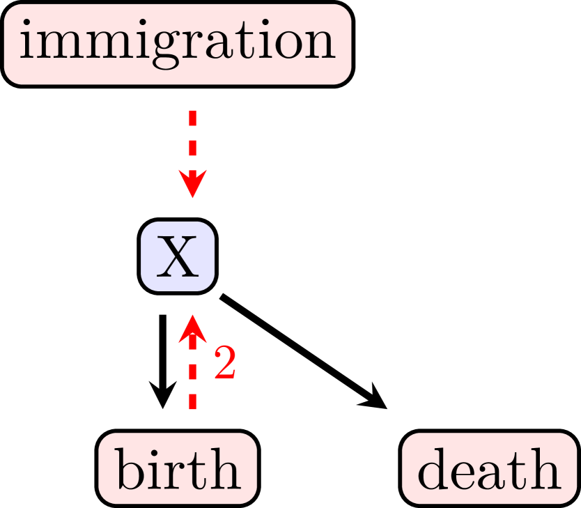
(a) Kendall’s process

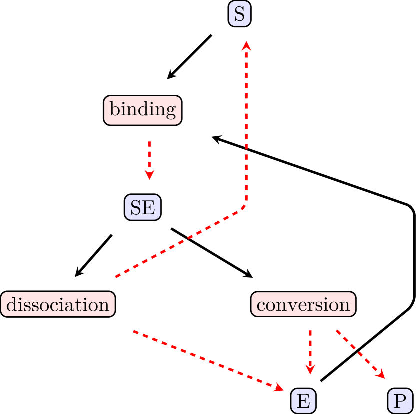
(b) Michaelis-Menten enzyme kinetics

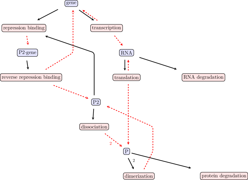
(c) Prokaryotic autoregulation

Figure 1: Petri net representations of (a) Kendall’s process, (b) the Michaelis-Menten model, and (c) a self-regulating gene network generated by BioSimulator.jl via the TikzGraphs package. Arrows connecting species to reaction denote how species enter into a reaction, and arrows from a reaction to a species denote how species are produced or deleted by the reaction. When the reaction produces more than 1 particle of a given species, its coefficient appears along the arrow connecting reaction to product species.

4.4 Simulation output

Output from stochastic simulation at a series of time points can be plotted as mean trajectories over time or as full distributions. BioSimulator.jl generates time series data for each species and stores it in a BioSimulator.jl provides a few convenient functions for visualization and summary statistics through the DataFrame provided by the DataFrames.jl package in Julia. The DataFrames.jl documentation provides examples for carrying out common operations, including data manipulation, computing summary statistics, and saving data to a file. DataFrame(result), where SimulationSummary. The resulting table has three types of columns. The trial columns indicate the time point and trial number of a record. The remaining columns are labelled according to the species or compartment name. One must load the DataFrames.jl package before converting simulation output to a minted[fontsize=]julia ¿ using DataFrames ¿ result = simulate(model, time = 50.0, epochs = 3, trials = 3) ¿ DataFrame(result) — Row — time — SE — S — P — E — trial — ——–—————-——–——–——–———-— — 1 — 0.0 — 0 — 301 — 0 — 130 — 1 — — 2 — 25.0 — 66 — 46 — 189 — 64 — 1 — — 3 — 50.0 — 12 — 0 — 289 — 118 — 1 — — 4 — 0.0 — 0 — 301 — 0 — 130 — 2 — — 5 — 25.0 — 63 — 38 — 200 — 67 — 2 — — 6 — 50.0 — 9 — 0 — 292 — 121 — 2 — — 7 — 0.0 — 0 — 301 — 0 — 130 — 3 — — 8 — 25.0 — 64 — 29 — 208 — 66 — 3 — — 9 — 50.0 — 17 — 0 — 284 — 113 — 3 —

4.5 Plotting

BioSimulator.jl provides convenient methods for visualizing simulation results through the Plots.jl package. Installing the Plots.jl package provides one with default recipes for plotting individual realizations, mean trajectories, and frequency histograms. The SimulationSummary to produce a figure depending on the value of :trajectory, :histogram. Consider the following examples:

• plot(result, plot_type=:meantrajectory, species=[”S”, ”E”], epochs = 100)

will plot the mean trajectories for the species $S$ and $E$ based on $100$ epochs. Error bars represent one standard deviation from the mean. itemize Plotting options can be mixed and matches based on the interface provided by Plots.jl. Users may consult the documentation of Plots.jl for help in further customizing figures.

5 Results

To illustrate the workflow of BioSimulator.jl, we provide three simple numerical examples using the SAL method unless otherwise specified. In each case, we set $\epsilon=0.03$, $\delta=2$, and $\beta=0.75$.

Example 1

Kendall’s process

Kendall’s birth, death, and immigration process is a continuous-time Markov chain governed by a birth rate $a_{1}$ per particle, a death rate $a_{2}$ per particle, and an immigration rate $a_{3}$. Let $X_{t}$ denote the count of a species $S$ at time $t$. The events (reactions)

$$\left\{\begin{aligned} S&\rightarrow S+S&\text{Birth}\\ S&\rightarrow 0&\text{Death}\\ 0&\rightarrow S&\text{Immigration}\end{aligned}\right.$$

occur with propensities $a_{1}\cdot S$, $a_{2}\cdot S$, and $a_{3}$, respectively. The Petri net in Figure 1 (a) shows the relationships between the particles and reactions. It allows the modeler to visualize the flow of particles through the network and check whether the set of reactions specified accurately captures the biological pathways being studied. The following code simulates this model in BioSimulator.jl:

⬇

using BioSimulator

\parmodel = Network(”Kendall’s Process”)

\parmodel <= Species(”S”, 5)

\parmodel <= Reaction(”Birth”, 2.0, ”S –> S + S”)

model <= Reaction(”Death”, 1.0, ”S –> 0”)

model <= Reaction(”Immigration”, 0.5, ”0 –> S”)

\parresult = simulate(model, StepAnticipation(), time=4.0, epochs=40, trials=100_000)

In addition to tracking the mean and variance, BioSimulator.jl enables the display of the full distribution of species counts. In this way, one can quantify the frequency of rare extinction events. Figure 2 summarizes results for the mean trajectory and distribution of species $S$ in Kendall’s process. At $t=4$, the average population is $300$, and in approximately $0.9$ percent of the simulations, the species has gone extinct by this time point. Figure 3 illustrates the trade-off in selecting large $\epsilon$ values in $\tau$-leaping methods, namely OTL and SAL. As $\epsilon$ decreases towards $0$, the distribution of $S$ at $t=4$ approaches the exact statistical results from the SSA. Note that the smaller $\epsilon$ values may force these $\tau$-leaping algorithms to perform slower than SSA because the proposed leap sizes become smaller than an SSA update. This means that each update wastes time computing a $\tau$ leap that is often rejected. On the other hand, large $\epsilon$ values tend to increase the number of bad leaps. In this case, $\tau$-leaping wastes time contracting the leap size until a suitable update emerges.

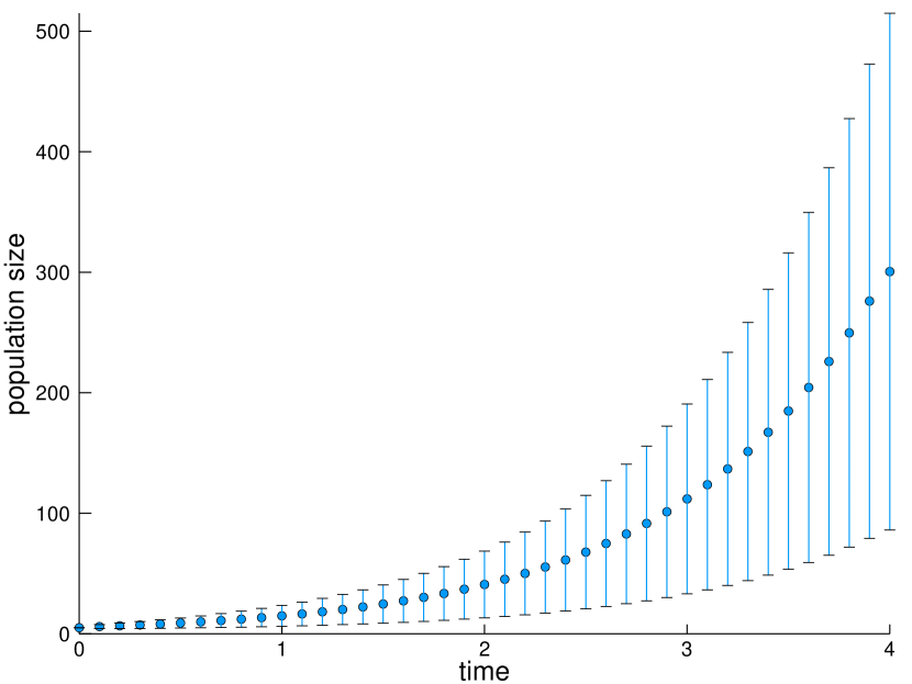
(a)

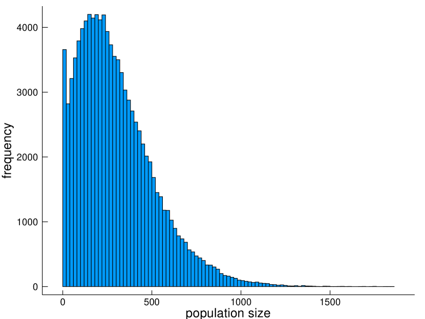
(b)

Figure 2: Kendall’s process with $\alpha=2.0$, $\mu=1.0$, and $\nu=0.5$ starting from $5$ particles. (a) Mean trajectory and distribution of species $S$ computed from $10^{5}$ SAL realizations. The light, colored region represents one standard deviation from the mean at each recorded point. (b) The histogram suggests extinction is possible at $t=4$ even though the mean value is approximately $300$.

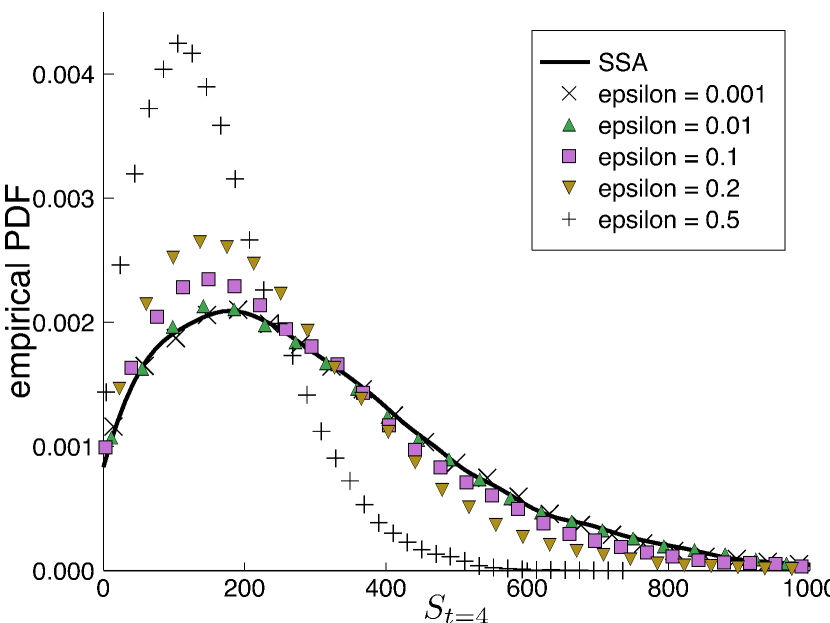
(a)

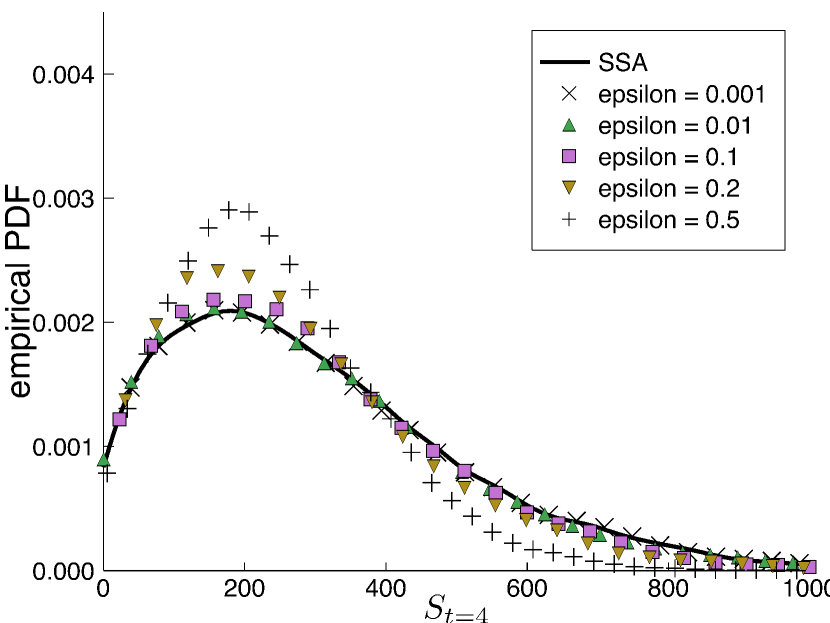
(b)

Figure 3: The distribution of $S$ in Kendall’s process at $t=4$ computed from $10^{5}$ realizations using (a) OTL and (b) SAL. SSA is used to derive an exact estimate of the distribution for comparison and is shown in black. The colored lines represent the resulting distribution under different values of $\epsilon$. Conservative values are generally safe, but may increase the clock time performance of a specific algorithm on a non-trivial model. In this example, the time to generate all $10^{5}$ realizations for SSA is approximately $5$ seconds. The running times for OTL are (in order of increasing $\epsilon$ value): $6$, $3$, $0.4$, $0.2$, and $0.1$ seconds. Similarly, the running times for SAL are: $9$, $6$, $0.2$, $0.1$, and $0.05$ seconds.

Example 2

Michaelis-Menten enzyme kinetics

Our next example, Michaelis-Menten enzyme kinetics, involves a combination of first- and second-order reactions. The system consists of a substrate S, an enzyme E, the substrate-enzyme complex SE, and a product P. The three reactions connecting them

$$\left\{\begin{aligned} S+E&\rightarrow SE&\text{Binding}\\ SE&\rightarrow S+E&\text{Dissociation}\\ SE&\rightarrow P+E&\text{Conversion}\end{aligned}\right.$$

represent binding of the substrate to an enzyme, dissociation of the substrate-enzyme complex, and conversion of the substrate into a product. These reactions have rates $a_{1}$, $a_{2}$, and $a_{3}$, respectively. The following code simulates this system under the initial conditions $S=301$, $E=130$, $SE=P=0$ and rate constants $a_{1}=0.00166$, $a_{2}=0.0001$, and $a_{3}=0.1$.

⬇

using BioSimulator

\parmodel = Network(”Michaelis-Menten”)

\parmodel <= Species(”S”, 301)

model <= Species(”E”, 130)

model <= Species(”SE”, 0)

model <= Species(”P”, 0)

\parmodel <= Reaction(”dimerization”, 0.00166, ”S + E –> SE”)

model <= Reaction(”dissociation”, 0.0001, ”SE –> S + E”)

model <= Reaction(”conversion”, 0.1, ”SE –> P + E”)

\parresult = simulate(model, StepAnticipation(), time = 50.0, epochs = 10_000, trials = 1_000)

Figure 1 (b) provides a Petri net representation of the model. Figure 4 (a) demonstrates mean trajectories and standard deviations for each of the reactant species over time. These mean trajectories match the dynamics predicted by a deterministic model. Figure 4 (b) shows the full distribution of species counts after $t=50$ time steps. The substrate is typically exhausted at $t=50$.

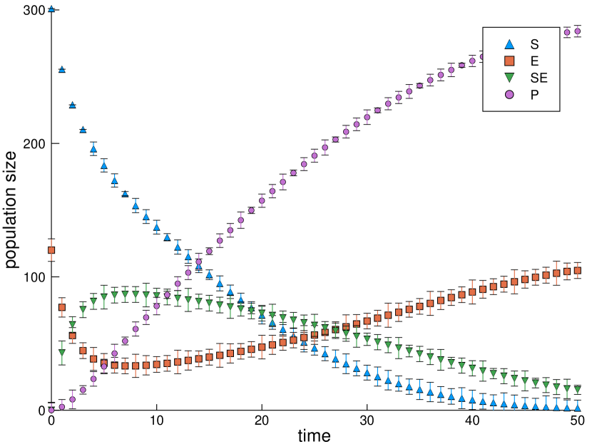
(a)

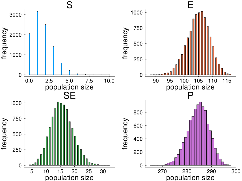
(b)

Figure 4: (a) Mean trajectory of each species in the Michaelis-Menten model using $10^{4}$ realizations. The region representing one standard deviation from the mean is small and suggests this network is not dominated by noise. (b) Population distributions for each species at $t=50$ generated from $10^{4}$ realizations.

Example 3

Auto-regulatory genetic network

The influence of noise at the cellular level is difficult to capture in deterministic models. Stochastic simulation is appropriate for the study of regulatory mechanisms in genetics, where key species may be present in low numbers. Figure 1 (c) is an example of a simplified negative auto-regulation network for a single gene, in the sense that the protein represses its own transcription. There are eight possible reactions: (1) gene transcription into RNA, (2) translation of the protein, (3) dimerization of the protein with itself, (4) dissociation of the protein dimer, (5) binding to the gene, (6) unbinding from the gene, (7) RNA degradation, and (8) protein degradation. There are five species to track — the free copies of the gene, transcribed RNA, protein molecules, dimer molecules, and blocked copies of the gene. The model is easily implemented in BioSimulator.jl:

⬇

using BioSimulator

\parmodel <= Network(”negative auto-regulation”)

\parmodel <= Species(”gene”, 10) # assume 10 copies of the gene are present

model <= Species(”RNA”, 0) # transcribed from the underlying gene

model <= Species(”P”, 0) # protein

model <= Species(”P2”, 0) # protein dimer

model <= Species(”P2_gene”) # gene repression

\parmodel <= Reaction(”transcription”, 0.01, ”gene –> gene + RNA”)

model <= Reaction(”translation”, 10.0, ”RNA –> RNA + P”)

model <= Reaction(”dimerization”, 1.0, ”P + P –> P2”)

model <= Reaction(”dissociation”, 1.0, ”P2 –> P + P”)

model <= Reaction(”repression binding”, 1.0, ”gene + P2 –> P2_gene”)

model <= Reaction(”reverse repression binding”, 10.0, ”P2_gene –> gene + P2”)

model <= Reaction(”RNA degradation”, 0.1, ”RNA –> 0”)

model <= Reaction(”protein degradation”, 0.01, ”P –> 0”)

\parresult = simulate(model, StepAnticipation(), Val(:full), time = 500.0, trials = 100)

RNA typically has a limited lifetime. Thus, the per particle reaction rates governing protein production are balanced to favor translation events following transcription. Moreover, the reaction rates for dimerization and dissociation reflect an assumption that the protein favors neither the monomer nor the dimer configuration.

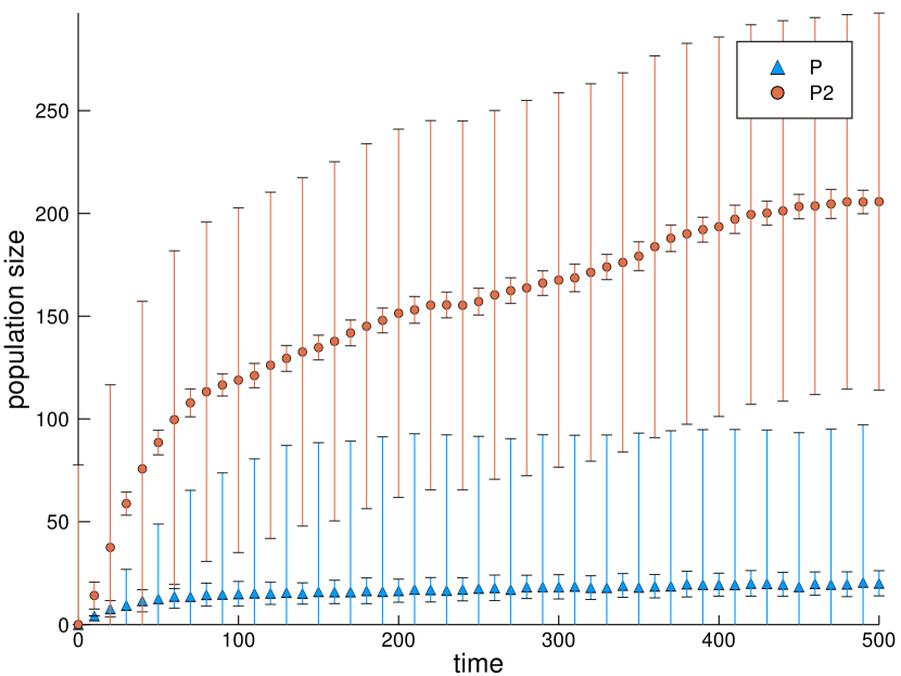
(a)

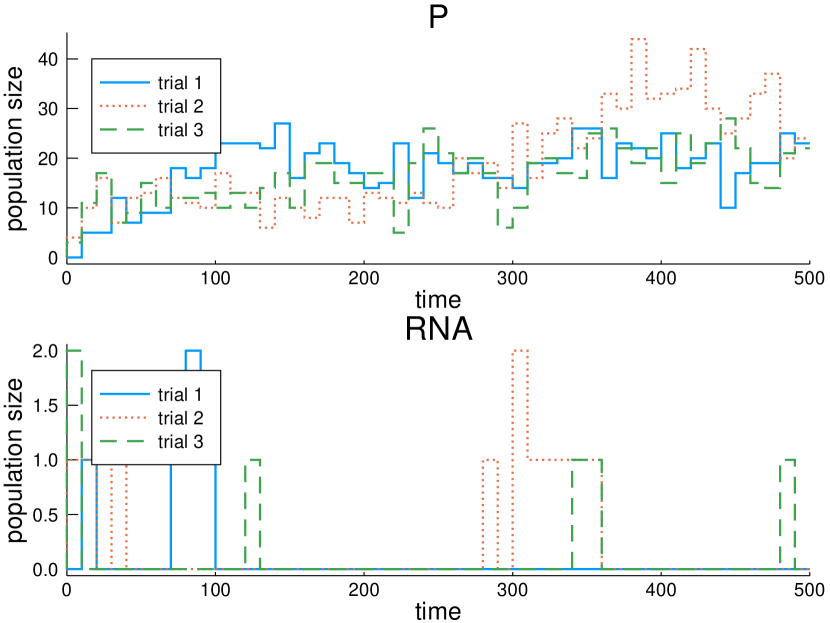
(b)

Figure 5: (a) Mean trajectories for the protein and dimer in a simple auto-regulatory gene network. The bars represent $1$ standard deviation away from the mean. (b) Full sample paths for the protein (top) and RNA (bottom). Note that the RNA sample path is sensitive to the number of epochs if one were using the fixed-interval option. Using a large window may fail to capture peaks in the output. This subtlety is important for qualitative model assessment.

Figure 5 (a) compares the mean behavior of the protein and the dimer over time with results from a deterministic model. Plotting individual trajectories for the protein level reveals strong stochastic fluctuations driven by the relative rarity of RNA. Figure 5 (b) highlights the influence of noise in the system’s dynamics.

5.1 Algorithm comparison

Here we compare the performance of BioSimulator.jl’s algorithms across the three examples from the previous sections. Each model is simulated using the same model parameters outlined in the previous examples. Each simulation task involves generating $100$ realizations. In the case of fixed-interval output, $1000$ epochs are used. The $\tau$-leaping algorithms use the default values $\epsilon=0.03$, $\delta=2$, and $\beta=0.75$. Table 5.1 records the averaged clock times reported by the Julia’s BenchmarkTools.jl package. Each simulation task is allotted $2$ minutes to generate $100$ samples of the running time. To be explicit, this means that the following command is executed at most $100$ times:

⬇

simulate(model, algname, output_option, time = tfinal, epochs = 1000, trials = 100)

Thus, these benchmarks reflect both the cost of generating a single realization, the efficiency of completing a typical simulation task, and the economy of choosing fixed-interval versus full simulation output. Results are based on a MacBook Pro with 2 GHz Intel Core i7 (4 cores) and 16 GB of RAM running macOS High Sierra 10.13.3.

Algorithm	Kendall’s process	Michaelis-Menten	Auto-regulation
SSA	$1.04\ (1.03-1.05)$	$0.783\ (0.788-0.808)$	$426\ (424-432)$
	$1.38\ (1.37-1.40)$	$0.918\ (0.909-0.936)$	$1809\ (1734-1860)$
FRM	$1.04\ (1.03-1.05)$	$0.863\ (0.853-0.874)$	$464\ (462-468)$
	$1.35\ (1.33-1.37)$	$0.983\ (0.973-1.000)$	$1597\ (1408-1645)$
NRM	$2.72\ (2.71-2.75)$	$3.11\ (3.08-3.15)$	$1589\ (1581-1597)$
	$2.99\ (2.96-3.02)$	$3.28\ (3.25-3.33)$	$2724\ (2553-2775)$
ODM	$1.02\ (1.01-1.03)$	$0.839\ (0.820-0.853)$	$409\ (407-412)$
	$1.34\ (1.32-1.37)$	$0.952\ (0.946-0.967)$	$1648\ (1437-1721)$
OTL	$0.722\ (0.715-0.726)$	$1.50\ (1.49-1.52)$	$1867\ (1863-1877)$
	$0.754\ (0.751-0.760)$	$1.64\ (1.63-1.67)$	$3038\ (2845-3087)$
SAL	$0.596\ (0.588-0.599)$	$0.989\ (0.985-0.996)$	$1422\ (1415-1441)$
	$0.607\ (0.604-0.612)$	$0.957\ (0.954-0.967)$	$2578\ (2398-2631)$

Table 2: Median runtimes and interquantile ranges (in milliseconds) for Example 1, Example 2, and Example 3 based on $1000$ samples of the command. Each simulation task generates $10$ realizations of the underlying stochastic model. For example, the median time to generate $10$ realizations of Kendall’s process using SSA is $1.04$ milliseconds. The first row in a cell is the benchmark result using the option for fixed-interval output. The second row indicates the timing result using the option for full simulation output.

The NRM performs the worst across the selected model. However, we note that BioSimulator.jl uses the a priority queue implementation from the DataStructures.jl package which may not be optimal for the method’s specific demands. Moreover, we take a naïve approach to building dependency graphs. The overhead from BioSimulator.jl’s dependency graphs is sufficiently large that in some cases most of the simulation is spent on this step. This warrants further review of our NRM implementation, although we expect an improved implementation to perform similarly to the FRM. Only the auto-regulation model may show improved performance for the NRM over SSA because the reaction channels for that model are not tightly coupled. Similarly, our ODM implementation may be inefficient based on its performance on the birth-death-immigration process. Both $\tau$-leaping algorithms perform poorly on the auto-regulation model. This is to be expected because neither OTL nor SAL handle separate time scales. Figure 5b shows that RNA transcription becomes a rare event as the protein dimer population grows. Similarly, the free and blocked gene copies are always present in relatively small quantities compared to the protein and protein dimer populations. Thus, protein dimerization and dissociation become the dominant reaction channels further along the time axis. These two reactions drive the dynamics of the system and therefore heavily influence the $\tau$-leap selection procedure. A natural consequence is that $\tau$-leaping methods have an increased likelihood of violating the leap condition in this regime and therefore bias the simulation toward infeasible states. This assertion is easily verified using the BioSimulator.jl. In fact, the leap condition violations are egregious to the point that the recovery mechanism requires thinning the leap several times per negative excursion. This suggests that reducing the leap size via the $\epsilon$ control parameter is likely to reduce the algorithm to SSA because leaps eventually become smaller than the expected Gillespie updates.

5.2 Software comparison

We compare BioSimulator.jl’s features and performance against three software packages: StochPy, StochKit2, and Gillespie.jl. The tools in the space of stochastic simulation are manifold and vary in their features and applications. Naturally, there are many omissions. Each software package is selected for its similarity to BioSimulator.jl. Specifically, these tools are domain-independent, general purpose Gillespie-like simulators. Table 3 summarizes the differences and similarities between these software tools. StochPy StochKit2 Gillespie.jl BioSimulator.jl Software characteristics: Language Python C++ Julia Julia Open-source Yes Yes Yes Yes GUI No via StochSS No No Jupyter integration Yes No Yes Yes Performance Fast Faster Faster Fastest Interactivity: Model editor No via StochSS No Yes Simulation interface Yes via StochSS Yes Yes Plotting Yes Limited No Yes Simulation features: Fixed-interval output via StochKit2 Yes No Yes Full output Yes Yes Yes Yes SBML support Yes Yes No No Readable input Yes No No Yes Parallelism No Yes No Yes Table 3: A summary of features across StochPy, StochKit2, Gillespie.jl, and BioSimulator.jl. Jupyter notebooks are human-readable documents that combine code, text, and figures into a single interactive report. In addition, we compare each software package on simulation speed across five different models: (a) Kendall’s process permits an analytic mean trajectory. This model serves as an easy speed test and a correctness check. (b) The Michaelis-Menten enzyme kinetics model provides a second simple speed test with multiple species. (c) The auto-regulation model serves a benchmark against an interesting biological application of stochastic simulation. (d) The dimer-decay model is an example of a small stiff system. It is featured in the literature as a $\tau$-leaping benchmark [7, 4]. (e) A yeast model from biology is another interesting stiff system used here as a benchmark. [8, 9, 32]. Initial conditions and other model parameters are deferred to supplementary information (Section A.1, Tables S1 - S5). Table 4 reports the benchmark results and includes the simulation parameters. Software StochPy StochKit2 Gillespie.jl BioSimulator.jl Method SSA SSA (dep. graph) SSA SSA Mode Serial Parallel Serial Serial Parallel Kendall’s process $174.31\ (173.81-174.95)$ $1.04\ (1.03-1.05)$ $0.56\ (0.48-0.66)$ $257\ (223-296)$ $1285\ (1280-1293)$ $1.38\ (1.37-1.40)$ $0.79\ (0.68-0.93)$ Michaelis-Menten $210.42\ (209.89-211.14)$ $0.783\ (0.788-0.808)$ $0.45\ (0.44-0.46)$ $214\ (213-216)$ $1.15\ (1.12-1.21)$ $0.918\ (0.909-0.936)$ $0.47\ (0.46-0.48)$ Auto-regulation $432\ (425-445)$ $426\ (424-432)$ $135\ (124-149)$ $8.23\ (7.87-8.75);\times 10^{4}$ $824\ (762-834)$ $1809\ (1734-1860)$ $211\ (193-240)$ Dimer-decay $216.98\ (216.52-217.68)$ $1.76\ (1.75-1.79)$ $0.81\ (0.80-0.82)$ $483\ (480-488)$ $2.68\ (2.66-2.84)$ $2.39\ (2.37-2.42)$ $1.03\ (1.02-1.05)$ Yeast $260\ (254-267)$ $2.56\ (2.53-2.63)$ $1.38\ (1.10-1.42)$ $469\ (465-474)$ $2.25\ (2.21-2.63)$ $2.92\ (2.89-2.99)$ $1.24\ (1.20-1.27)$ Table 4: Median runtimes and interquantile ranges for StochPy, StochKit2, Gillespie.jl, and BioSimulator across selected models based on $1000$ samples, reported in milliseconds (ms). Each sample measured the time to generate $10$ realizations of a given stochastic process. Results using fixed-interval and fixed output options are recorded in the first and second rows of each cell, respectively. Each simulation tool is used with its default settings. For example, StochKit2 automatically parallelizes simulation tasks involving multiple realizations and uses a dependency graph by default. We note that both StochKit2 and BioSimulator.jl used $8$ threads for the parallel simulation benchmarks. Direct comparisons based on these results are not possible, in the sense that slower performance does not necessarily indicate a particular tool is poorly implemented. Rather, our results reflect natural trade-offs in optimizing software for particular goals. Note: The StochPy benchmark on the auto-regulation model is based on only $100$ samples.

5.3 Package availability

BioSimulator.jl is available on GitHub (https://github.com/alanderos91/BioSimulator.jl). All source code is readily available to view, download, and distribute under the MIT license. We also maintain a documentation manual via GitHub Pages (https://alanderos91.github.io/BioSimulator.jl/stable/).

6 Discussion

BioSimulator.jl simplifies interactive stochastic modeling by virtue of being contained within a single programming language. Every aspect of the modeling workflow --- model specification, simulation, and analysis --- is handled by Julia and its type system. Here we discuss these three aspects of our simulation software and compare its features and timing benchmarks with other packages. StochPy and BioSimulator.jl are mainly interactive simulation tools meant to be used in Read-Eval-Print Loop (REPL) environments and Jupyter notebooks, but they stand out in that they can also be used as libraries like StochKit2. BioSimulator.jl’s model specification interface is flexible enough to allow a user to build up a model using for loops and other language features. StochPy and StochKit2 mainly rely on input files whose main advantage is model sharing. Model editing interfaces can be built around standardized formats and indeed such tools exist; StochSS includes a graphical user interface that feeds into StochKit2. The strength of BioSimulator.jl’s model interface is the flexibility afforded by Julia’s features as it facilitates rapid model prototyping. An additional benefit of our implementation is that models can be packaged into functions by defining a wrapper. This allows one to share models through minted[fontsize=,samepage]julia function birth_death_process(S; birth_rate = 2.0, death_rate = 1.0, immigration_rate = 0.5) model = Network("Kendall’s Process") model <= Species("S", S) model <= Reaction("Birth", birth_rate, "S --> S + S") model <= Reaction("Death", death_rate, "S --> 0") model <= Reaction("Immigration", immigration_rate, "0 --> S") return model end Here S to specify an initial condition. The variables death_rate, and birth_death_process(5) builds up the model with $S_{0}=5$ and the default reaction rate constants. Many models are implemented using data standards independent of software and programming languages. One notable standard is the Systems Biology Markup Language (SBML) [3]. SBML addresses crucial details such as parameter units, compartment sizes, and kinetic rate laws in a standardized format. An interface to SBML is required in order to connect BioSimulator.jl to existing software, enable thorough comparisons, and facilitate model sharing in a standardized way. StochPy and StochKit2 stand out in this regard because these tools provide an interface to SBML. We anticipate adopting the SBML standard in future versions of our software. StochKit2 is primarily a command-line tool and a software development package. This makes StochKit2 highly reusable since other programs, such as model editors or simulation packages, can interface with it. In fact, one of StochPy’s features is its ability to call StochKit2 for tau-leaping. The main commands are tau_leaping

. At the start of a simulation job, StochKit2 performs an analysis to select a suitable algorithm based on the model structure. For example, using the Gillespie.jl is a fast stochastic simulation tool for visualizing results and computing quantities of interest, but it requires a modest programming effort. Without a model editor, it requires the user to specify the net change increments $\mathbf{v}^{j}$ and propensity functions $r_{j}(\mathbf{x})$ for each reaction $j$. This approach places a burden on users, especially those unfamiliar with Julia or any similar programming language. A benefit of this interface is that non-mass action propensities are automatically supported since a user must hard-code these for the software. Unlike the other tools, Gillespie.jl does not yet have an interface for running multiple simulations, and so collecting the results from independent simulations requires some effort from a user. While the main simulation functions are similar, Gillespie.jl and BioSimulator.jl have the advantage of Julia’s type system and multiple-dispatch. When used correctly, these two language features allow one to write powerful abstractions around scientific computing problems that Julia leverages to generate highly optimized instructions. The JuMP.jl and DifferentialEquations.jl packages are exemplars in this regard and serve as a testament to Julia’s advantages [11, 31]. The benchmarking results from Table 4 show that BioSimulator.jl is competitive with StochKit2. While we are pleased with BioSimulator.jl’s performance, one can only speculate on the precise meaning of these benchmarks without an intimate understanding of implementation details. Julia provides a theoretical competitive performance edge for Gillespie.jl and BioSimulator.jl over the Python software. StochPy’s timings may be slower due to the fact that it records a greater amount of information. In addition to recording the state vector after each step, StochPy offers the option to store reaction channel information such as propensity values and event waiting times. While fixed-interval output provides StochKit2 and BioSimulator.jl with a slight performance boost, the results between StochPy and BioSimulator.jl using the full output option suggest that the performance gap is in fact wide. StochKit2 and BioSimulator.jl each support running parallel simulations. StochKit2 automates this feature; the software defaults to parallelism if a user’s machine supports it. However, BioSimulator.jl’s implementation is nearly automatic thanks to Julia’s abstractions for parallelism. Table 4 shows that BioSimulator.jl is an order of magnitude faster on each example in the serial case, except for the auto-regulation model. This warrants further investigation. All four packages support varying degrees of simulation output analysis. Gillespie.jl and BioSimulator.jl offer automatic time series visualization. We improve upon Gillespie.jl by providing helper functions for additional visualization tools, such as histograms and mean trajectories, as well as integration with the Plots.jl ecosystem. Our goal is to emulate StochKit2 / StochSS and StochPy in their support for more sophisticated analysis tools.

7 Conclusion

In a biological system, interacting feedback loops can make mathematical analysis intractable and create challenges in choosing an optimal set of experiments to probe system behavior. Combining experiments and stochastic simulation of complex biological systems promotes model validation and the design of promising experiments. The user-friendly nature of BioSimulator.jl encourages the use of stochastic simulation, eliminates effort spent on modifying simulation code, reduces errors during model specification, and allows visualization of system interactions via Petri Nets. Tracking trajectories and distributions of interacting species over time helps modelers decide between deterministic and stochastic models. Future developments of BioSimulator.jl include

• support for non-mass action kinetics,

• adopting SBML as an input format,

• extending the SAL algorithm implementation using higher order Taylor expansions,

• implementing additional exact and approximate simulation algorithms from the literature,

• incorporating spatial effects, and

• implementing hybrid methods that integrate stochastic simulation with deterministic modeling.

The Julia language provides an ideal environment for this purpose. Its syntax allows one to write mathematical code in a natural way and facilitates fast prototyping. In particular, the integration with the IJulia package encourages code sharing and reproducible work. Furthermore, its interactive environment is well-suited for novice programmers. The package ecosystem in Julia provides software for visualization, statistical analysis, optimization, differential equations, and probability distributions. Emerging computational tools in Julia can only increase BioSimulator.jl’s strengths over time.

References

- Andrews [2017] Steven S. Andrews. Smoldyn: particle-based simulation with rule-based modeling, improved molecular interaction and a library interface. Bioinformatics, 33(5):710–717, 2017. doi: 10.1093/bioinformatics/btw700. URL http://dx.doi.org/10.1093/bioinformatics/btw700.
- Bezanson et al. [2017] Jeff Bezanson, Alan Edelman, Stefan Karpinski, and Viral B. Shal. Julia: A fresh approach to numerical computing. SIAM Review, 59(1):65–98, 2017. doi: 10.1137/141000671. URL https://doi.org/10.1137/141000671.
- Bornstein et al. [2008] Benjamin J. Bornstein, Sarah M. Keating, Akiya Jouraku, and Michael Hucka. LibSBML: an API Library for SBML. Bioinformatics, 24(6):880–881, 2008. doi: 10.1093/bioinformatics/btn051. URL http://dx.doi.org/10.1093/bioinformatics/btn051.
- Cao and Petzold [2008] Yang Cao and Linda Petzold. Slow-scale tau-leaping method. Computer Methods in Applied Mechanics and Engineering, 197(43):3472 – 3479, 2008. ISSN 0045-7825. doi: https://doi.org/10.1016/j.cma.2008.02.024. URL http://www.sciencedirect.com/science/article/pii/S0045782508000959. Stochastic Modeling of Multiscale and Multiphysics Problems.
- Cao et al. [2004] Yang Cao, Hong Li, and Linda Petzold. Efficient formulation of the stochastic simulation algorithm for chemically reacting systems. Journal of Chemical Physics, 121(9), 2004. doi: 10.1063/1.1778376. URL https://doi.org/10.1063/1.1778376.
- Cao et al. [2005] Yang Cao, Daniel T. Gillespie, and Linda R. Petzold. Avoiding negative populations in explicit poisson tau-leaping. The Journal of Chemical Physics, 123(5):054104, 2005. doi: 10.1063/1.1992473. URL https://doi.org/10.1063/1.1992473.
- Cao et al. [2006] Yang Cao, Daniel T. Gillespie, and Linda R. Petzold. Efficient step size selection for the tau-leaping simulation method. Journal of Chemical Physics, 124(4), 2006. doi: 10.1063/1.2159468. URL https://doi.org/10.1063/1.2159468.
- Chou et al. [2008] Ching-Shan Chou, Qing Nie, and Tau-Mu Yi. Modeling robustness tradeoffs in yeast cell polarization induced by spatial gradients. PLOS ONE, 3(9):1–16, 09 2008. doi: 10.1371/journal.pone.0003103. URL https://doi.org/10.1371/journal.pone.0003103.
- Drawert et al. [2010] Brian Drawert, Michael J. Lawson, Linda Petzold, and Mustafa Khammash. The diffusive finite state projection algorithm for efficient simulation of the stochastic reaction-diffusion master equation. The Journal of Chemical Physics, 132(7):074101, 2010. doi: 10.1063/1.3310809. URL https://doi.org/10.1063/1.3310809.
- Drawert et al. [2016] Brian Drawert, Andreas Hellander, Ben Bales, Debjani Banerjee, Giovanni Bellesia, Bernie J. Daigle, Jr., Geoffrey Douglas, Mengyuan Gu, Anand Gupta, Stefan Hellander, Chris Horuk, Dibyendu Nath, Aviral Takkar, Sheng Wu, Per Lötstedt, Chandra Krintz, and Linda R. Petzold. Stochastic Simulation Service: Bridging the gap between the computational expert and the biologist. PLOS Computational Biology, 12(12):1–15, 12 2016. doi: 10.1371/journal.pcbi.1005220. URL https://doi.org/10.1371/journal.pcbi.1005220.
- Dunning et al. [2017] Iain Dunning, Joey Huchette, and Miles Lubin. JuMP: A modeling language for mathematical optimization. SIAM Review, 59(2):295–320, 2017. doi: 10.1137/15M1020575. URL https://github.com/JuliaOpt/JuMP.jl.
- El Samad et al. [2005] Hana El Samad, Mustafa Khammash, Linda Petzold, and Dan Gillespie. Stochastic modelling of gene regulatory networks. International Journal of Robust and Nonlinear Control, 15(15):691–711, 2005. doi: 10.1002/rnc.1018. URL https://onlinelibrary.wiley.com/doi/abs/10.1002/rnc.1018.
- Elowitz et al. [2002] Michael B. Elowitz, Arnold J. Levine, Eric D. Siggia, and Peter S. Swain. Stochastic gene expression in a single cell. Science, 297(5584):1183–1186, 2002. ISSN 0036-8075. doi: 10.1126/science.1070919. URL http://science.sciencemag.org/content/297/5584/1183.
- Frost [2016] Simon DW Frost. Gillespie.jl: Stochastic simulation algorithm in julia. Journal of Open Source Software, 1:42, 2016. doi: 10.21105/joss.00042. URL https://doi.org/10.21105/joss.00042.
- Gibson and Bruck [1999] Michael A. Gibson and Jehoshua Bruck. Efficient exact stochastic simulation of chemical systems with many species and many channels. Journal of Physical Chemistry, 104(9), 1999. doi: 10.1021/jp993732q. URL https://doi.org/10.1021/jp993732q.
- Gillespie [1976] Daniel T Gillespie. A general method for numerically simulating the stochastic time evolution of coupled chemical reactions. Journal of Computational Physics, 22(4):403 – 434, 1976. ISSN 0021-9991. doi: https://doi.org/10.1016/0021-9991(76)90041-3. URL http://www.sciencedirect.com/science/article/pii/0021999176900413.
- Gillespie [1977] Daniel T. Gillespie. Exact stochastic simulation of coupled chemical reactions. The Journal of Physical Chemistry, 81(25):2340–2361, 1977. doi: 10.1021/j100540a008. URL https://doi.org/10.1021/j100540a008.
- Gillespie [2001] Daniel T. Gillespie. Approximate accelerated stochastic simulation of chemically reacting systems. Journal of Chemical Physics, 115(4), 2001. doi: 10.1063/1.1378322. URL https://doi.org/10.1063/1.1378322.
- Gillespie and Petzold [2003] Daniel T. Gillespie and Linda R. Petzold. Improved leap-size selection for accelerated stochastic simulation. Journal of Chemical Physics, 19:8229–8234, 2003. doi: 10.1063/1.1613254. URL https://doi.org/10.1063/1.1613254.
- Gillespie et al. [2013] Daniel T. Gillespie, Andreas Hellander, and Linda R. Petzold. Perspective: Stochastic algorithms for chemical kinetics. The Journal of Chemical Physics, 138(17):170901, 2013. doi: 10.1063/1.4801941. URL https://doi.org/10.1063/1.4801941.
- Golightly, Andrew and Gillespie, Colin S. [2013] Golightly, Andrew and Gillespie, Colin S. Simulation of Stochastic Kinetic Models, pages 169–187. Humana Press, Totowa, NJ, 2013. ISBN 978-1-62703-450-0. doi: 10.1007/978-1-62703-450-0˙9. URL https://doi.org/10.1007/978-1-62703-450-0_9.
- Harris et al. [2016] Leonard A. Harris, Justin S. Hogg, José-Juan Tapia, John A. P. Sekar, Sanjana Gupta, Ilya Korsunsky, Arshi Arora, Dipak Barua, Robert P. Sheehan, and James R. Faeder. BioNetGen 2.2: advances in rule-based modeling. Bioinformatics, 32(21):3366–3368, 2016. doi: 10.1093/bioinformatics/btw469. URL http://dx.doi.org/10.1093/bioinformatics/btw469.
- Higham [2008] Desmond J. Higham. Modeling and simulating chemical reactions. SIAM Review, 50(2), 2008. doi: 10.1137/060666457. URL https://doi.org/10.1137/060666457.
- Hoops et al. [2006] Stefan Hoops, Sven Sahle, Ralph Gauges, Christine Lee, Jürgen Pahle, Natalia Simus, Mudita Singhal, Liang Xu, Pedro Mendes, and Ursula Kummer. COPASI—a COmplex PAthway SImulator. Bioinformatics, 22(24):3067–3074, 2006. doi: 10.1093/bioinformatics/btl485. URL http://dx.doi.org/10.1093/bioinformatics/btl485.
- Lange [2003] Kenneth Lange. Applied Probability. Springer-Verlag, 2003.
- Lopez et al. [2013] Carlos F Lopez, Jeremy L Muhlich, John A Bachman, and Peter K Sorger. Programming biological models in Python using PySB. Molecular Systems Biology, 9(1), 2013. ISSN 1744-4292. doi: 10.1038/msb.2013.1. URL http://msb.embopress.org/content/9/1/646.
- Maarleveld et al. [2013] Timo R. Maarleveld, Brett G. Olivier, and Frank J. Bruggeman. StochPy: A comprehensive, user-friendly tool for simulating stochastic biological processes. PLOS ONE, 8(11), 2013. doi: 10.1371/journal.pone.0079345. URL https://doi.org/10.1371/journal.pone.0079345.
- Mauch and Stalzer [2011] S. Mauch and M. Stalzer. Efficient formulations for exact stochastic simulation of chemical systems. IEEE/ACM Transactions on Computational Biology and Bioinformatics, 8(1):27–35, Jan 2011. ISSN 1545-5963. doi: 10.1109/TCBB.2009.47. URL https://doi.org/10.1109/TCBB.2009.47.
- McAdams and Arkin [1997] H. H. McAdams and A. Arkin. Stochastic mechanisms in gene expression. Proc. Natl. Acad. Sci. U.S.A., 94(3):814–819, Feb 1997. URL https://www.ncbi.nlm.nih.gov/pmc/articles/PMC19596. [PubMed Central:PMC19596] [PubMed:9023339].
- Pineda-Krch [2008] Mario Pineda-Krch. GillespieSSA: Implementing the gillespie stochastic simulation algorithm in r. Journal of Statistical Software, Articles, 25(12):1–18, 2008. ISSN 1548-7660. doi: 10.18637/jss.v025.i12. URL https://www.jstatsoft.org/v025/i12.
- Rackauckas and Nie [2017] Christopher Rackauckas and Qing Nie. DifferentialEquations.jl -– a performant and feature-rich ecosystem for solving differential equations in julia. Journal of Open Research Software, 5(1):15, May 2017. doi: 10.5334/jors.151. URL http://juliadiffeq.org/.
- Roh et al. [2011] Min K. Roh, Bernie J. Daigle, Dan T. Gillespie, and Linda R. Petzold. State-dependent doubly weighted stochastic simulation algorithm for automatic characterization of stochastic biochemical rare events. The Journal of Chemical Physics, 135(23):234108, 2011. doi: 10.1063/1.3668100. URL https://doi.org/10.1063/1.3668100.
- Sehl et al. [2009] Mary E. Sehl, Alexander L. Alekseyenko, and Kenneth L. Lange. Accurate stochastic simulation via the step anticipation -leaping (SAL) algorithm. Journal of Computational Biology, 16:1195–1208, 2009. doi: 10.1089/cmb.2008.0249. URL https://dx.doi.org/10.1089%2Fcmb.2008.0249.
- Voliotis et al. [2016] Margaritis Voliotis, Philipp Thomas, Ramon Grima, and Clive G. Bowsher. Stochastic simulation of biomolecular networks in dynamic environments. PLOS Computational Biology, 12(6):1–18, 06 2016. doi: 10.1371/journal.pcbi.1004923. URL https://doi.org/10.1371/journal.pcbi.1004923.
- Wilkinson [2006] Darren J. Wilkinson. Stochastic Modeling for Systems Biology. Chapman & Hall/CRC Press, Boca Raton, FL, 1 edition, 2006. ISBN 9781439837726.