Efficient simulation of finite-temperature open quantum systems

Abstract

Chain-mapping techniques in combination with the time-dependent density matrix renormalization group are a powerful tool for the simulation of open-system quantum dynamics. For finite-temperature environments, however, this approach suffers from an unfavorable algorithmic scaling with increasing temperature. We prove that the system dynamics under thermal environments can be non-perturbatively described by temperature-dependent system-environmental couplings with the initial environment state being in its pure vacuum state, instead of a mixed thermal state. As a consequence, as long as the initial system state is pure, the global system-environment state remains pure at all times. The resulting speedup and relaxed memory requirements of this approach enable the efficient simulation of open quantum systems interacting with highly structured environments in any temperature range, with applications extending from quantum thermodynamics to quantum effects in mesoscopic systems.

Quantum systems are never completely isolated and the interaction with surrounding uncontrollable degrees of freedom can modify significantly their dynamical properties. In some cases the environment can be assumed to be memoryless, in which case master equations of Lindblad form provide an accurate effective description of the resulting open-system dynamics Carmichael (1993); Breuer and Petruccione (2002); Gardiner and Zoller (2004); Rivas and Huelga (2012). Generally, however, the description of the evolution of open quantum systems (OQSs) requires to take into full account the environmental degrees of freedom and their interaction with the system. This becomes particularly important, when the system-environment coupling is not weak, and the environment reorganization process occurs on a time scale which is comparable to the system dynamics – a situation that is ubiquitous in soft or condensed matter, nanothermodynamics and quantum biology Huelga and Plenio (2013); Rivas et al. (2014); Breuer et al. (2016); de Vega and Alonso (2017). In this case, the OQS dynamics is not accessible to either analytical methods (apart from very few specific instances Luczka (1990); Hu et al. (1992); Garraway (1997); Fisher and Breuer (2007); Smirne and Vacchini (2010); Diósi and Ferialdi (2014); Ferialdi (2016)), nor effective master equation approaches and more refined numerical techniques are thus needed.

Over the last two decades, a variety of numerically exact approaches for the simulation of open quantum systems have been proposed. These methods allowed for the description of features that were not accurately described by approximate methods, such as the Markov, Bloch-Redfield or perturbative expansion techniques Breuer and Petruccione (2002). In particular, the Time Evolving Density operator with Orthogonal Polynomials (TEDOPA) Prior et al. (2010); Chin et al. (2010) algorithm is a certifiable method Woods et al. (2015) for the nonperturbative simulation of OQS that has found application for the description of a variety of open quantum systems Prior et al. (2010, 2013); Chin et al. (2013). TEDOPA belongs to the class of chain-mapping techniques Hughes et al. (2009); Prior et al. (2010); Chin et al. (2010); Martinazzo et al. (2011); Woods et al. (2014); Ferialdi and Dürr (2015), and is closely related to Lanczos tridiagonalization (see de Vega et al. (2015) and references therein); these techniques are based on a unitary mapping of the environmental modes onto a chain of harmonic oscillators with nearest-neighbor interactions. The main advantage of this mapping is the more local entanglement structure which results in an improved efficiency of density matrix renormalization group (DMRG) methods White (1992). While TEDOPA is very efficient at zero temperature, a regime that is hard to access by other methods such as hierarchical equations of motion (HEOM) Tanimura and Kubo (1989); Ishizaki and Fleming (1999); Tanimura (2006) and path integral methods Feynman (1948); Makri (1992); Nalbach et al. (2010), its original formulation suffers from a unfavorable scaling when increasing the temperature of the bosonic bath. Because of this, other approaches, such as HEOM, are currently the method of choice in the high temperature regime.

In this work we derive a formulation of TEDOPA for finite-temperature bosonic environments that allows for its extension to arbitrary temperatures without loss of efficiency. Our approach relies on the equivalence between the reduced dynamics of an OQS interacting with a finite-temperature bosonic environment characterised by some spectral density and the dynamics of the same system interacting with a zero temperature environment and a suitably modified spectral density Diósi et al. (1998); Yu (2004); Blasone et al. (2011); de Vega and Bañuls (2015), and further exploits fundamental properties of the theory of orthogonal polynomials Gautschi (1994); Chin et al. (2010); Woods et al. (2014).

Spectral density thermalization.— Consider a quantum system $S$ interacting with a bosonic environment; for each environmental mode at frequency $\omega\geq 0$ the annihilation and creation operators $a_{\omega},a_{\omega}^{\dagger}$ satisfy the commutation relations $[a_{\omega},a_{\omega^{\prime}}^{\dagger}]=\delta_{\omega\omega^{\prime}},[a_{\omega},a_{\omega}^{\prime}]=[a_{\omega}^{\dagger},a_{\omega^{\prime}}^{\dagger}]=0,\forall\omega,\omega^{\prime}\geq 0$. The system-environment total Hamiltonian is defined by ($\hbar=1$)

$$H_{SE} =H_{S}+H_{E}+H_{I}$$ (1)

$$H_{E} =\int_{0}^{+\infty}d\omega\ \omega a_{\omega}^{\dagger}a_{\omega};\,\,\,H_{I}=A_{S}\otimes\int_{0}^{+\infty}d\omega\ O_{\omega},$$ (2)

where $H_{S}$ is the free system (arbitrary) Hamiltonian and $H_{E},\ H_{I}$ describe, respectively, the free evolution of the environmental degrees of freedom and the bilinear system-environment interaction Leggett et al. (1987a). In what follows we assume that $O_{\omega}$ is a self-adjoint operator and, in particular, is given by:

$$O_{\omega}=\sqrt{J(\omega)}X_{\omega}=\sqrt{J(\omega)}\left(a_{\omega}+a_{\omega}^{\dagger}\right),$$ (3)

while $A_{S}$ is a generic operator on the open system $S$. The function $J(\omega):\mathbb{R}^{+}\mapsto\mathbb{R}^{+}$ is defined by the product of the interaction strength between the system and the environmental mode at frequency $\omega$ and the mode density, and is usually referred to as the spectral density (SD) Breuer and Petruccione (2002).

At time $t=0$, system and environment are assumed to be in a factorized state $\rho_{SE}(0)=\rho_{S}(0)\otimes\rho_{E}(0)$, where $\rho_{S}(0)$ is an arbitrary (pure or mixed) initial state of the system, $\rho_{E}(0)=\bigotimes_{\omega}\exp(-\beta\omega a_{\omega}^{\dagger}a_{\omega})/\mathcal{Z_{\omega}}$ is the thermal state of the environment at inverse temperature $\beta=1/k_{B}T$ and $\mathcal{Z_{\omega}}=\operatorname{Tr}_{E}(\exp(-\beta\omega a_{\omega}^{\dagger}a_{\omega}))$. Under these assumptions, the open system state $\rho_{S}(t)=\operatorname{Tr}_{E}(\rho_{SE}(t))$ at a generic time $t$ is entirely determined by the spectral density $J(\omega)$ and the inverse temperature $\beta$ Feynman and Vernon (1963); van Kampen (1974); Breuer and Petruccione (2002); Gasbarri and Ferialdi (2018). In fact, $\rho_{S}(t)$ is fully determined by the two-time correlation function

$$S(t) =\int_{0}^{+\infty}d\omega\ \left\langle O_{\omega}(t)O_{\omega}(0)\right\rangle_{\rho_{\omega}(\beta)}$$ (4)

$$=\int_{0}^{+\infty}d\omega\ J(\omega)\left[e^{-i\omega t}(1+n_{\omega}(\beta))+e^{i\omega t}n_{\omega}(\beta)\right],$$

where $O_{\omega}(t)=\exp(iH_{E}t)O_{\omega}\exp(-iH_{E}t)$ is the environmental interaction operator evolved at time $t$ via the free Hamiltonian $H_{E}$ and $n_{\omega}(\beta)=\left\langle a_{\omega}^{\dagger}a_{\omega}\right\rangle_{\rho_{\omega}(\beta)}=(\exp(\beta\omega)-1)^{-1}$. It is then clear that given two environments with the same two-time correlation functions, the corresponding reduced dynamics coincide Carmichael (1993); Breuer and Petruccione (2002); Tamascelli et al. (2018).

If we formally extend the integral in (4) to the whole real axis and define the anti-symmetrized spectral density $J^{\text{ext}}(\omega)=\text{sign}(\omega)J(|\omega|)$ with support on the whole real axis May and Kühn (2004), the two-time correlation function can be reexpressed in the form

$$S(t)=\int_{-\infty}^{+\infty}d\omega\ \frac{J^{\text{ext}}(\omega)}{2}\left(1+\coth\left(\frac{\beta\omega}{2}\right)\right)e^{-i\omega t}.$$ (5)

It is crucial to note that this function can be associated with an extended bosonic environment, with positive and negative frequencies, governed by $H_{E^{\text{ext}}}=\int_{-\infty}^{+\infty}d\omega\omega a_{\omega}^{\dagger}a_{\omega}$, which is initially in the vacuum state (i.e., $a_{\omega}|0\rangle\,\,\forall\omega\in\mathbb{R}$) and which interacts with the system via the interaction Hamiltonian $H_{I}(\beta)=A_{S}\otimes\int_{-\infty}^{+\infty}d\omega\ \sqrt{J_{\beta}(\omega)}X_{\omega}$, and that now involves a temperature-dependent spectral density (T-SD)

$$J_{\beta}(\omega)=\frac{J^{\text{ext}}(\omega)}{2}\left(1+\coth\left(\frac{\beta\omega}{2}\right)\right).$$ (6)

We conclude that the reduced dynamics in the presence of an initial thermal state of the environment and a global Hamiltonian as in Eqs.(1) and (2) is the same as the one resulting from an initial vacuum state of the extended environment and a coupling governed by the new spectral density defined in Eq.(6). Note that, in contrast to previous approaches Diósi et al. (1998); Yu (2004); Blasone et al. (2011); de Vega and Bañuls (2015), we achieved this equivalence by suitably redefining the spectral density, which is the central object in TEDOPA. Importantly, the relationship between the original thermal chain and the pure state chain with the temperature-dependent spectral density can be formulated in terms of a unitary equivalence, which, in principle, allows one to recover the state of the full system-environment state in the original picture at any time $t$ sup .

Thermalized TEDOPA.— TEDOPA Prior et al. (2010); Chin et al. (2010); Tamascelli et al. (2015); Kohn et al. (2018a) relies on the theory of orthogonal polynomials Gautschi (2004) to provide an analytical unitary transformation mapping the original star-shaped system-environment model into a one dimensional configuration Chin et al. (2010). New modes with creation and annihilation operators $c_{n}^{\dagger}$ and $c_{n}$ are defined as $c_{n}^{(\dagger)}=\int_{0}^{+\infty}d\omega\ U_{n}(\omega)a_{\omega}^{(\dagger)}$ using the unitary transformation $U_{n}(\omega)=\sqrt{J(\omega)}p_{n}(\omega)$ where $J(\omega)$ is an input (arbitrary) SD, and $p_{n}(\omega),\ n=0,1,\ldots$ are orthogonal polynomials with respect to the measure, i.e. the positive valued function, $d\mu(\omega)=J(\omega)d\omega$ on $\mathbb{R}^{+}$. Thanks to the three-term recurrence relation satisfied by the orthogonal polynomials $p_{n}(\omega)$, the $H_{SE}$ Hamiltonian in Eq.(1) is mapped Chin et al. (2010) into a chain Hamiltonian $H^{C}=H_{S}+H_{I}^{C}+H_{E}^{C}$ with

$$H_{I}^{C} =\kappa_{0}A_{S}(c_{0}+c_{0}^{\dagger})$$

$$H_{E}^{C} =\sum_{n=0}^{+\infty}\omega_{n}c_{n}^{\dagger}c_{n}+\sum_{n=1}^{+\infty}\kappa_{n}(c_{n}^{\dagger}c_{n-1}+H.c.).$$ (7)

After the unitary transformation, thus, the system interacts only with the new mode $c_{0}^{(\dagger)}$, and all the interactions are nearest neighbour. The mode frequencies $\omega_{n}$ and couplings $\kappa_{n}$ are related to the recurrence coefficients for the polynomials $p_{n}(\omega)$ and can be computed either analytically or via stable numerical routines Gautschi (1994); Chin et al. (2010). The crucial observation at this point is that, assuming $\int_{0}^{+\infty}d\omega J(\omega)/\omega<\infty$, i.e. finite reorganization energy, the temperature-dependent spectral density in Eq.(6) defines a measure $\mu_{\beta}(\omega)=J_{\beta}(\omega)d\omega$, with support extending, by construction, over the whole real axis. Hence, there exists a family of polynomials $p_{\beta,n}$ which are orthogonal with respect to $d\mu_{\beta}$ and we can define the unitary transformation

$$U_{\beta,n}(\omega) =\sqrt{J_{\beta}(\omega)}p_{\beta,n}(\omega)$$ (8)

$$c_{\beta,n}^{\dagger} =\int_{-\infty}^{+\infty}d\omega\ U_{\beta,n}(\omega)a_{\omega}^{\dagger},$$ (9)

and follow the same procedure as before. The resulting Hamiltonian has the same form as Eq.(7), with the modes $c_{n}^{(\dagger)}$ replaced by $c_{\beta,n}^{(\dagger)}$ and new coefficients $\omega_{\beta,n},\kappa_{\beta,n}$ related to the polynomials $p_{\beta,n}$. The unitary transformations $U_{n}(\omega)$ and $U_{\beta,n}(\omega)$ respectively determine the initial state of the chain: for standard TEDOPA the thermal state of the environment is mapped to the thermal state of the chain $\rho_{E}^{C}(\beta)=\exp(-\beta H_{E}^{C})/\mathcal{Z}_{E}^{C}$, while the vacuum state of the extended environment is mapped to a (factorized) vacuum pure state of the chain.

Impact on simulations.— As long as $\rho_{S}(0)$ is a pure state, the global state of system and chain in the T-SD approach remains pure for $\forall t\geq 0$. This has a major impact on the simulation of the system dynamics via time-dependent DMRG techniques White and Feiguin (2004); Rommer and Östlund (1997), such as the time-evolving-block-decimation algorithm (TEBD) Vidal (2003, 2004); Zwolak and Vidal (2004). From now on we will refer to TEDOPA with T-SD approach as T-TEDOPA. In order to fully appreciate the advantage provided by T-TEDOPA, here we discuss the main features of its scaling properties; a more detailed comparison of the complexity of the standard and thermalized methods is reported in the SM sup .

In order to enable computer simulations, both the length of the harmonic chain and the local dimension of the environmental oscillators must be truncated. These truncations must be chosen such that finite-size effects remain negligible during the simulation interval $[0,t_{\text{max}}]$. For a chain of length $N$ and local dimension $d$, the complexity of the standard TEDOPA approach scales as $O(Nt_{\text{max}}(d^{2}\chi)^{3})$, where $\chi$ is the bond dimension, a TEBD parameter that is related to the amount of correlations in the simulated system. On the other hand, the complexity for T-TEDOPA will be given by $O(N^{\prime}t_{\text{max}}(d^{\prime}\chi^{\prime})^{3})$, where the primed letters emphasize that, in general, the local dimension, the chain length and the bond dimension will be different from the standard case. Clearly, the reduced complexity of T-TEDOPA stems mainly from the fact that only pure states are involved in the simulation, whereas for standard TEDOPA mixed states are needed.

In addition, the local dimensions required to faithfully represent thermal state of the chain scales unfavorably with the temperature, and, as a consequence, $d^{\prime}$ can be taken significantly smaller than $d$ sup . For all the dynamics taken into account here, the decrease of the local dimension in the T-TEDOPA overcompensates by itself the increase of the chain length (we usually set $N^{\prime}\approx 2N$ due to an increased propagation speed in the chain) and of the bond dimension (we used at most $\chi^{\prime}\approx\sqrt{2}\chi$) sup .

It is important to note that the Matrix Product Operator (MPO) representation of the chain cannot be determined analytically in general and its preparation requires a considerable additional computational overhead. This step is clearly not required by T-TEDOPA, since the factorized vacuum state can be straightforwardly represented via Matrix Product States (MPS). It is worth noting that the approach developed in de Vega and Bañuls (2015) shares some features of the T-TEDOPA. It allows to use pure instead of mixed states as well, but maps the positive and negative frequency environmental degrees of freedom into two separate chains. This results in a locally 2-dimensional tensor network with a consequent considerable increase of the simulation complexity, as discussed extensively in sup . As a last, but practically relevant observation, we note that T-TEDOPA does not require any change in the already existing and optimized TEDOPA codes, since it only needs a modification of the chain coefficients.

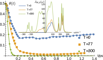
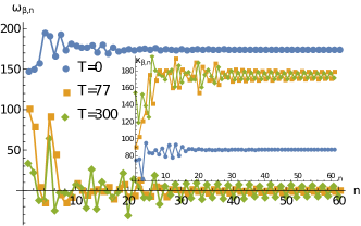
Figure 1: Coherence dynamics $\theta(t)$ for a TLS subject to pure dephasing induced by a reservoir modelled by $J_{W}(\omega)$ at $T=0,77,300\,{\rm K}$. Markers represent T-TEDOPA results; analytic results, defined as in the text, are shown as solid lines. In the inset, the corresponding T-SD $J_{W,\beta}(\omega)$. (b) Chain coefficients $\omega_{\beta,n}$ and $\kappa_{\beta,n}$ (inset) corresponding to $J_{W,\beta}$ for $T=0,77,300\,{\rm K}$.

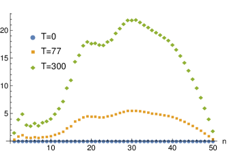
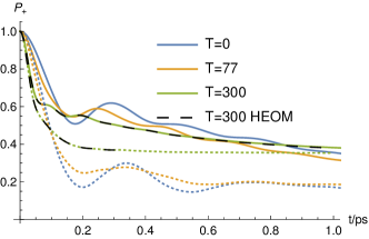
Figure 2: (a) TEDOPA chain initialization. Average occupation number of the oscillators of a chain obtained by the standard mapping of $J_{W}(\omega)$; the values have been obtained via the procedure described in sup . (b) Simulation results for a model dimeric system. The expectation value of $P_{+}=|+_{D}\rangle\langle+_{D}|$ as a function of time at different temperatures shows the dynamical effect of the environmental noise on the lifetime of coherent superpositions of (electronic) quantum states. Dotted lines correspond to a structured spectral form $J_{W}(\omega)$, while solid lines correspond to $J_{W}^{\prime}(\omega)$. HEOM Tanimura and Kubo (1989); Ishizaki and Fleming (1999); Tanimura (2006) results are shown (dashed black lines) for comparison at $300\,{\rm K}$ (see SM sup for more details).

Case study.— In order to illustrate the main features of T-TEDOPA, we present two examples where we consider environments with a structured SD $J_{W}(\omega)$, consisting of a broad background plus three Lorenzian peaks. This type of spectral density is characteristic of pigment-protein complexes, where electrically coupled pigments are subject to the structured environment provided by intra-pigment and protein vibrations Chandrasekaran et al. (2015); Olbrich et al. (2011).

The accuracy of the results provided by T-TEDOPA is clearly apparent when comparing the simulation results with a solvable model. Consider a two level system (TLS) subject to a pure dephasing dynamics. The environment and interaction Hamiltonians are defined as in Eqs.(2) and (3) with $A_{S}=(1+\sigma_{z})/2$ and $J(\omega)=J_{W}(\omega)$. The T-SD in Eq.(6) at $T=0,77$ and $300\,{\rm K}$ are shown in the inset of Fig.1(a), while its full definition is provided in sup . We imposed a hard cut-off $\omega_{c}=350$$\,{\rm cm}^{-1}$ such that $\int_{\omega_{c}}^{\infty}d\omega J_{W}(\omega)/\omega$ becomes negligible ($<10^{-4}{\rm cm}^{-1}$). Assume that the initial state of the TLS is a coherent superposition of the form $|+\rangle=(|0\rangle+|1\rangle)/\sqrt{2}$. In an interaction picture, the system’s coherence is given by $\theta(t)=\exp(-\gamma(t))/2$, with $\gamma(t)=\int_{0}^{\omega_{c}}d\omega J_{W}(\omega)\coth\left({\omega}/{2k_{B}T}\right)\left[(1-\cos\omega t)/{\omega^{2}}\right]$ Breuer and Petruccione (2002) where $\gamma(t)$ is often referred to as the decoherence function.

As clearly shown in Fig.1(a), T-TEDOPA accurately reproduces the behavior of the coherence for $t<1.4\,\text{ps}$, with maximum error $<10^{-4}$. As shown in Fig.1(b), the T-TEDOPA chain coefficients depend, as expected, on the temperature $T$. In particular, we observe that the coupling $\kappa_{\beta,0}$ between the system and the first oscillator in the chain increases with $T$. For any assigned SD $J(\omega)$, we obtain $\kappa_{\beta,0}=||J_{\beta}||_{1}=\sqrt{\int_{-\omega_{c}}^{\omega_{c}}d\omega J_{\beta}(\omega)}$, which is a non-decreasing function of $T$. Moreover, the behaviour of the chain parameters $\kappa_{\beta,n}$ and $\omega_{\beta,n}$ as functions of $n$ becomes more and more jagged as $T$ increases, inducing an effective detuning between nearest neighboring sites in the initial part of the chain. This configuration leads to non-negligible back-scattering of an excitation located initially at the first site of the chain sup . A systematic analysis of these processes, which underpin the non-Markovian part of the dynamics, and their non-trivial temperature dependence will be the subject of a future work. Here we simply point out that this configuration results in the first sites of the T-TEDOPA chain having a higher occupation number. This allows a gradual decrease in the local dimensions $d_{n}^{\prime}$ of the $n=1,\ldots,N$, which significantly reduces the simulation complexity. For example, for the simulation at $T=300\,$K, the dimension $d_{n}^{\prime}=d_{\text{max}}^{\prime}-n(d_{\text{max}}^{\prime}-2)/N$ with $d_{\text{max}}^{\prime}=12$ ($\chi=50$) led to converged results. We notice, moreover, that the chain coefficients $\omega_{\beta,n}$ and $\kappa_{\beta,n}$ tend to converge for large $n$ to the expected asymptotic values Gautschi (2004); Woods et al. (2014): if $[a(\beta),b(\beta)]$ is the support of $J_{\beta}(\omega)$, then $\omega_{\beta,n}\stackrel{{\scriptstyle n\to\infty}}{{\longrightarrow}}(a(\beta)+b(\beta))/2$ whereas $\kappa_{\beta,n}^{2}\stackrel{{\scriptstyle n\to\infty}}{{\longrightarrow}}(b(\beta)-a(\beta))^{2}/16$. Since the support is $[0,\omega_{c}]$ at $T=0$ and $[-\omega_{c},\omega_{c}]$ at $T>0$, this means that at finite temperature T-TEDOPA will in general require longer chains than standard TEDOPA. This increase in length, however, leads to a constant factor increase in the T-TEDOPA complexity and is significantly overcompensated by the possibility of starting from the vacuum state. Indeed, as mentioned before, the local dimension of the standard TEDOPA scales unfavorably with the temperature, as we exemplify in Fig.2(a) where we show the average occupation number of the chain consisting of $N=50$ oscillators. It is clear that the minimal local dimension of the oscillator chain must be chosen much larger than the average occupation number to allow for an accurate representation of the chain thermal state. It is not surprising that the sole preparation of the chain thermal state at $T=77\,{\rm K}$ required one week of computation for the choice $d=8$ (16 Intel Xeon E5-2630v3 cores), while the $T=300\,{\rm K}$ T-TEDOPA simulation (Fig.1(a)) required only 8 hours using the same cores sup .

As a second example, we discuss the simulation of a form of the water-soluble chlorophyll-protein (WSCP) homodimer, a model system for the study of pigment-protein interactions and for which there exists a rather complete experimental characterization, both structurally and in terms of its linear and nonlinear optical responses Renger et al. (2011); Alster et al. (2014). We model the WSCP dimer as two identical TLSs with interaction Hamiltonian $H_{S}=H_{D}=\lambda\sigma_{+}^{L}\sigma_{-}^{R}+\text{H.c.}$, where $\lambda=69\,\text{cm}^{-1}$ is the cross coupling term and $\sigma_{\pm}^{L,R}$ are the spin raising and lowering operators $(\sigma_{x}^{L,R}\pm i\sigma_{y}^{R,L})/2$ on the left ($L$) and right ($R$) TLS. When restricted to the single excitation subspace, $H_{D}$ admits the eigenvalues $\pm 69\,\text{cm}^{-1}$ with corresponding eigenstates $|\pm_{D}\rangle$. Each TLS interacts with a local harmonic bath. The two baths are independent but described by the same spectral density $J_{W}(\omega)$ used so far. The interaction Hamiltonian is $H_{I}=H_{I}^{L}+H_{I}^{R}$ with $H_{I}^{L(R)}$ defined as in Eq.(2) with $A_{S}^{L(R)}=(1+\sigma_{z}^{L(R)})/2$. Since the overall Hamiltonian conserves the excitation number, the evolved state belongs to the space spanned by $|\pm_{D}\rangle$. Fig.2(b) shows the evolution of the projection $P_{+}=|+_{D}\rangle\langle+_{D}|$ as a function of time, when the system starts from $\rho_{S}(0)=|+_{D}\rangle\langle+_{D}|$, for two different spectral densities, namely the full spectral density $J_{W}(\omega)$ and $J_{W}^{\prime}(\omega)$ where only the background is considered. The simulation at $300\,$K required $d_{\text{max}}^{\prime}=20$, $\chi=180$. A detailed discussion of the influence of the Lorentzian contribution to the reduced system dynamics and the comparison with actual experiments is beyond the scope of this work, but our results already show the capability of the method to make predictions across the whole temperature range and for highly structured spectral densities.

Conclusion and outlook.— In this work we have presented a new method, T-TEDOPA, for the efficient, accurate and certifiable simulation of open quantum system dynamics at arbitrary temperatures. The central insight was a suitable redefinition of the environmental spectral density which allowed for the use of a zero temperature environment in place of a finite temperature environment without affecting the system dynamics. This allows for using MPS in place of MPO for the description of the harmonic chain of environmental oscillators. As a consequence, we obtain a significant reduction in the scaling of the algorithmic complexity as compared to state-of-the-art chain mapping techniques and orders of magnitude reductions in computation time. By construction, T-TEDOPA can be implemented as a plug-in procedure by the already existing and highly optimized TEDOPA codes, which can now be used to efficiently simulate open quantum system dynamics across the entire temperature range.

Our approach is particularly relevant whenever one wants to provide a quantitative description of open-system dynamics in the presence of structured and non-perturbative environments, such as those commonly encountered in quantum biology Huelga and Plenio (2013), nanoscale thermodynamics Vinjanampathy and Anders (2016) or condensed-matter systems Leggett et al. (1987a), as well as situations where the effect of environmental noise has to be identified accurately to discriminate it from possible fundamental decoherence in high-precision tests of the quantum superposition principle Bassi et al. (2013); Arndt and Hornberger (2014), or be exploited as building block in other methods, such as the Transfer Tensor scheme Cerrillo and Cao (2013); Rosenbach et al. (2016). Future research will be devoted to the extension of the T-TEDOPA method to more general types of system-bath interactions.

We thank Felipe Caycedo-Soler and Ferdinand Tschirsich for many useful discussions; we acknowledge support by the ERC Synergy grant BioQ, the QuantERA project NanoSpin, the EU projects AsteriQS and HYPERDIAMOND, the BMBF projects DiaPol, the John Templeton Foundation and the CINECA-LISA project TEDDI.

Supplemental Material to “Efficient simulation of finite-temperature open quantum systems”

D. Tamascelli^1,2, A. Smirne¹, J. Lim¹ S. F. Huelga¹, and M. B. Plenio¹

March 8, 2024

Supplemental Material

.1 Chain occupation number

At finite temperature, TEDOPA requires the determination of the thermal state of the chain of environment oscillators in MPO representation. This thermal state is determined as the fixed point of the evolution in imaginary time under the environment Hamiltonian Zwolak and Vidal (2004). For this time consuming procedure to be accurate, the local dimension of each oscillator in the chain must be chosen sufficiently large to allow for an accurate representation of the thermal state. Here, we describe a general procedure to determine the chain occupation number, which in Sect..4 will also allow us to give an estimate of the local dimension that must be considered at the different temperatures.

Given the chain coefficients $\omega_{n},\kappa_{n}$ associated by the chain mapping to an assigned spectral density $J(\omega)$, and the number of chain sites $N$, chosen as not to have finite size effects, a lower bound on the local dimension of the oscillators can be provided by the following procedure. The chain Hamiltonian (see eq. (7) in the main text)

$$H_{E}^{C}=\sum_{n=0}^{N-1}\omega_{n}c_{n}^{\dagger}c_{n}+\sum_{j=1}^{N-2}\kappa_{n}(c_{n}c_{n+1}^{\dagger}+H.c.),$$ (10)

can be rewritten as

$$H_{E}^{C}=\text{\boldmath$c$}^{\dagger}A\text{\boldmath$c$}$$ (11)

with $\text{\boldmath$c$}=\left(c_{0},c_{1},\ldots,c_{N-1}\right)^{T}$

$$A=\left(\begin{array}[]{c c c c c}\omega_{0}&\kappa_{1}&0&\dots&0\\ \kappa_{1}&\omega_{1}&\kappa_{2}&\dots&0\\ \dots&\dots&\dots&\dots&\dots\\ 0&0&0&\kappa_{N-2}&\omega_{N-1}\end{array}\right).$$ (12)

The three-diagonal real matrix $A$ can be diagonalized $A=U^{T}DU$ with $D=\operatorname{{diag}}\left(\omega_{0}^{\prime},\omega_{1}^{\prime},\ldots,\omega_{N}^{\prime}\right)$ and $U$ being a unitary operator $U^{T}=U^{-1}$. Stated otherwise, the chain admits $N$ normal modes with frequency $\omega_{n}^{\prime},\ n=1,2,\ldots,N$ and creation/annihilation operators defined as linear combinations of of the operators $c_{n},c_{n}^{\dagger}$ by

$$b =U\text{\boldmath$c$},$$ (13)

$$\text{\boldmath$b$}^{\dagger} =\text{\boldmath$c$}^{\dagger}U^{T}.$$ (14)

By linearity, the average occupation number of the $n$-th chain oscillator $\langle c_{n}^{\dagger}c_{n}\rangle_{\beta}$ at inverse temperature $\beta$ can be determined from the average occupation number of the chain normal modes $\langle b_{n}^{\dagger}b_{n}\rangle_{\beta}=1/(e^{\beta\omega_{n}}-1)$ of the normal modes $\omega_{n}^{\prime}$ through

$$\langle c_{n}^{\dagger}c_{n}\rangle_{\beta}=\sum_{k=0}^{N-1}\left(U_{k,n}\right)^{2}\langle b_{k}^{\dagger}b_{k}\rangle_{\beta},$$ (15)

where $U_{k,n}$ is the element in the $k$-th row and $n$-th column of $U$. Since the thermal state is Gaussian it is in principle possible to determine its state, and the expectation of any observable on the chain analytically. In particular, it would be possible to determine the average occupation of each level of each oscillator. However, by simply using the convexity of expectation values, it is possible to claim that if $\langle c_{n}^{\dagger}c_{n}\rangle_{\beta}=j$ then at least the lowest $\lceil j\rceil$ levels are occupied. This suffices to provide an estimate for the scaling of the required local dimension of the chain oscillators with the temperature, see also Sect..4.

.2 Length of the chain

For a predetermined simulation time $t_{\text{max}}$, we need to determine the required chain length $N$ to prevent reflections off the end of the chain to influence the system dynamics. Since the coefficients derive from orthogonal polynomials with respect to a temperature dependent measure $d\mu_{\beta}(\omega)=J_{\beta}(\omega)d\omega$, the value of $N$ depends on both $t_{max}$ and the temperature. As already shown in Fig.1b of the main text, for large $N$ the chain coefficients $\omega_{\beta,n}$ and $\kappa_{\beta,n}$ converge towards asymptotic values that depend only on the support of $J_{\beta}(\omega)$. For large $N$, in the quasi-homogeneous region of the chain, an excitation propagates at a speed proportional to $\kappa_{\beta,\infty}\stackrel{{\scriptstyle\text{def}}}{{=}}\lim_{n\to\infty}\kappa_{\beta,n}$. As $\kappa_{\beta,\infty}$ tends to grow with temperature, this explains the need for longer chains for T-TEDOPA at finite temperatures as compared to standard TEDOPA. A better estimate of the required chain length for assigned $J_{\beta}(\omega)$ and $t_{\text{max}}$ can be obtained from a heuristic technique that turns out to be quite reliable.

The propagation of an excitation injected by the system into the chain can be studied by a quantum walk like approach. We consider an initial state where a single excitation is located at the first site of the chain of environmental oscillators and remove the system-environment coupling. Since the chain Hamiltonian conserves the number of excitations, the evolution of the chain is confined to the single excitation sector. We can therefore use the Hamiltonian

$$H_{qw}=\sum_{n=0}^{M}\omega_{\beta,n}|n\rangle\langle n|+\sum_{n=1}^{M-1}\kappa_{\beta,n}(|n+1\rangle\langle n|+\text{H.c.}),$$ (16)

where $|n\rangle$ indicates a chain with the excitation located at the $n$-th TLS and $M$. The evolved state $|\psi_{qw}(t)\rangle=\sum_{n=0}^{M}\alpha_{n}(t)|n\rangle$ can be easily computed by solving a linear system of $M$ coupled equations. The optimal length $N$ can then be estimated by direct inspection of the coefficients $|\alpha_{n}(t)|^{2}$ for different values of $M$. The optimal value corresponds to the smallest $N$ such that the excitation after reflection off the end of the chain has not reached the first site with an appreciable probability in the time interval $[0,t_{\text{max}}]$. There is a good agreement between the position of the propagation front provided by such an approach and the actual propagation in the thermalized chains at all the considered temperatures, as exemplified by Fig.1 (a) and (b).

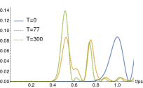
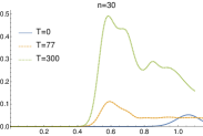
Figure 3: (a) The probability $|\alpha_{30}(t)|^{2}$ of finding the single excitation, initially located in the first site $|\psi_{0}\rangle=\sum_{n=1}^{60}\delta_{n,1}$ of an $N=60$ sites chain governed by the Hamiltonian (16) of the main text. (b) The actual average occupation number, as a function of time, of the 30-th chain oscillator at different temperatures.

.3 Excitation dynamics of the first chain sites

Another fundamental feature of T-TEDOPA is the accumulation of excitation in the oscillators that are closest to the system. This effect is monotonous in the temperature, as shown in Fig.4. This can be explained qualitatively by looking at the couplings and the energies in this region. First of all, as already remarked in the main text, the system-chain coupling is a monotonous function of $T$ (see Fig.1(b) of the main text). This implies that, at least in the early stages of the evolution, with increasing temperature, more excitations are created in the first few chain sites by the interaction with the system. Moreover, in the same region the site energies and couplings exhibit significant disorder that is increasing with temperature. Therefore, excitations created by the interaction with the system cannot propagate ballistically in this part of the chain and get partially localized, as can be observed in Fig.4. This behavior is fundamental for a chain initialized in its vacuum state to achieve, at the level of the system-dynamics, the same dynamics as a thermalized chain. We will examine this aspect of the dynamics in more detail in a forthcoming work.

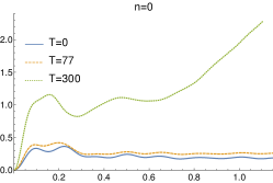
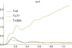
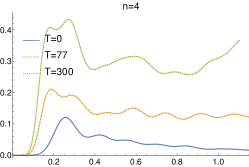
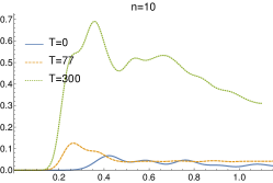
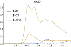
Figure 4: The average occupation number of the $n$-th site of the T-SD as a function of time and at different temperatures. (a) $n=0$, (b) $n=1$, (c) $n=4$, (d) $n=10$, (e) $n=20$. The plot of the same quantity for $n=30$ is shown in Fig.3(b) of the main text.

.4 TEDOPA vs T-TEDOPA algorithmic complexity: details

Here, relying on the analyses in the previous Sections, we provide a more detailed description of the computational complexity scaling of TEDOPA and T-TEDOPA. We will consider only the complexity of the real-time evolution part and disregard the determination of the initial state of the thermalized chain required by standard TEDOPA.

For a spectral density $J(\omega)$ and inverse temperature $\beta$, we indicate by the chain truncation $N$, local dimension $d$ and bond dimension $\chi$ that achieve converged results in the simulation interval $[0,t_{\text{max}}]$ for standard TEDOPA, and by $N^{\prime}$, $d^{\prime}$, $\chi^{\prime}$ the analogous parameters for T-TEDOPA. As proved in Schollwöck (2011), the computational complexity of TEDOPA is $O(Nt_{\text{max}}(d^{2}\chi)^{3})$. The term $(d^{2}\chi)^{3}$ is due to the computational cost of the two-site update part of TEBD Schollwöck (2011), which requires singular value decompositions (SVDs) of $d^{2}\chi$ matrices (for simplicity we are assuming all the local and bond dimensions to be constant along the chain) and represents the real bottleneck of TEBD which absorbs, on the average, about 90% of the computational time. By adopting a randomized version of SVD (RSVD) Tamascelli et al. (2015); Kohn et al. (2018), the complexity of TEDOPA can be reduced to $O(Nt_{\text{max}}(d^{2}\chi)^{2})$. Even with RSVD, the simulations at high temperature are computationally highly demanding, since, $d$ needs to be taken quite large at high $T$.

As mentioned in the main text, with T-TEDOPA the matrices that need to be handled are much smaller for two reasons. First of all the states to be represented are pure, so that MPS representation suffices. Moreover, typically, the local dimension $d^{\prime}$ can be chosen significantly smaller than $d$ at finite $T$. Local dimensions $d^{\prime}=6,8,12$ for the for the monomer simulation at $T=0,77$ and $300K$ respectively, for example, provided converged results, while the mere representation of the chain thermal states would have required much larger local dimension. The availability of tight estimates of the T-TEDOPA optimal local dimension would clearly be a most useful tool, and stringent mathematical results will be discussed elsewhere.

In addition to this, as discussed in the previous section, a further significant decrease in the computational complexity can be reached via the use of a non-uniform local dimension $d^{\prime}(n),\ n=1,2,\ldots,N^{\prime}$. On the one hand, the occupation of the first sites in the chain, where localization of the population injected from the system occurs, is larger than the occupation in the remaining part of the chain. Our numerical experience shows that with the choice $d^{\prime}(n)=d^{\prime}_{\text{max}}-n(d^{\prime}_{\text{max}}-2)/N^{\prime}$ always leads to converged results. While the asymptotic scaling is left invariant by this choice, the actual constants are much smaller than for the case of a uniform local dimension $d^{\prime}(n)=d^{\prime}_{\text{max}}$. This has a significant impact on the simulation time. In the original TEDOPA scheme, an analogous fine tuning of the local dimension cannot be achieved with the same efficiency. While the excitations that the system injects into the chain will still concentrate in the first few sites of the chain, they distribute faster across the chain leading to significant occupation numbers along the entire chain, with a maximum around the half of the chain (see Fig.2(a) of the main text as an example). This reduces strongly the possibility to decrease the local dimension of the oscillators without detailed knowledge about the system-environment dynamics.

On the other hand, while in TEDOPA the system-chain coupling $\kappa_{0}$ and the chain parameters $\omega_{n},\kappa_{n}\ n=1,2,\ldots$ are fixed, and only the initial state of the chain was a function of temperature, in T-TEDOPA all the $\omega_{n},\kappa_{n}$ are temperature dependent. In particular, the system-chain coupling is a monotonically increasing with temperature, $\kappa_{\beta,0}=||J_{\beta}||_{1}=\sqrt{\int_{-\omega_{c}}^{\omega_{c}}d\omega J_{\beta}(\omega)}$ and $\kappa_{\beta,0}\stackrel{{\scriptstyle\beta\to 0}}{{\longrightarrow}}\sqrt{2}||J||_{1}$. At high temperatures, therefore, the system-chain coupling is larger for T-TEDOPA than for standard TEDOPA. It is difficult to obtain a precise estimate for the required $\chi$ ($\chi^{\prime}$) for T-TEDOPA and standard TEDOPA and it is rather difficult to provide any general quantitative statement about the relation between the bond dimensions in the two approaches. However, for all the numerical examples that we have considered here, we always obtained T-TEDOPA converged results by setting at most $\chi^{\prime}=1.4\chi$.

Finally, due to the higher asymptotic value of the coupling between nearest-neighbour oscillators in the thermalized case, one has to take a longer chain, i.e. $N^{\prime}>N$ (see the discussion in Sect..2). In our numerical examples we have found that $N^{\prime}\approx 2N$ was always sufficient All in all, however, the use of a smaller local dimension, along with the possibility to decrease it along the chain, amply compensate by itself the increased bond dimension and chain length.

We conclude this section with a technical, but relevant, remark. T-TEDOPA differs from TEDOPA only in the computation of the chain coefficients. As such, it can be used with existing and optimized TEDOPA codes. In TEDOPA, however, the workload related to the SVD decomposition and other matrix operations on the typically large (MPO) matrices was distributed over the available computing cores via multi-threaded executions at an open-MP level (e.g. multi-threaded Intel Math-Kernel-Library https://software.intel.com/en-us/intel mkl ). With the reduced dimension of the matrices needed by T-TEDOPA, on the other side, such approach would not fully exploit the available computational resources. This suggests to use the same computing cores at an openMP https://www.openmp.org or MPI https://www.mpi forum.org level: independent two-sites updates can be distributed over different threads or processes running on multi-core architectures. A benchmark of our TEDOPA code with openMP parallelization showed a linear speedup with the number of available cores w.r.t. single-core executions. A TEDOPA code with MPI layer, distributing the workload over different computational nodes, is currently under development.

.5 WSCP spectral density

The spectral density $J_{W}(\omega)$ is the combination of a broad background at low frequency and three Lorentzian peaks at high frequency. More specifically,

$$J_{W}(\omega) =\sum_{k=1}^{3}J_{LN,k}(\omega)+\sum_{m=1}^{3}J_{L,m}(\omega),$$ (17)

$$J_{LN,k}(\omega) =\frac{S_{k}}{\sigma_{k}\sqrt{2\pi}}\omega\exp\left\{-\frac{\left[\ln(\omega/\omega_{k})\right]^{2}}{2\sigma_{k}^{2}}\right\},$$ (18)

$$J_{L,m}(\omega) =\frac{4\gamma_{m}\Omega_{m}g_{m}(\Omega_{m}^{2}+\gamma_{m}^{2})\omega}{\pi\left[\gamma_{m}^{2}+(\omega+\Omega_{m})^{2}\right]\left[\gamma_{m}^{2}+(\omega-\Omega_{m})^{2}\right]}.$$ (19)

The low frequency part (or backgound) is the combination Rosnik and C. (2015) of three log-normal functions with with $S_{1}=0.39,S_{2}=0.23,S_{3}=0.23$, $\sigma_{1}=0.4,\sigma_{2}=0.25,\sigma_{3}=0.2$, $\omega_{1}=26\text{cm}^{-1},\omega_{2}=51\text{cm}^{-1},\omega_{3}=85\text{cm}^{-1}$. The three Lorentzian peaks have all the same width $\gamma_{k}=\gamma=5\text{cm}^{-1}$, and are centered in $\Omega_{1}=181\text{cm}^{-1},\Omega_{2}=221\text{cm}^{-1},\Omega_{3}=240\text{cm}^{-1}$ and have weights $g_{1}=0.0173,g_{2}=0.0246,g_{3}=0.0182$.

.6 Thermofield, T-SD and double-chain method

In this section we discuss in more detail the relation between the approach developed in this work using a thermal spectral density and a pure state environment and the methods developed in Diósi et al. (1998); Yu (2004); Blasone et al. (2011); de Vega and Bañuls (2015) which rely on the thermofield formalism. On the one hand, this will allow us to show how to recover, at least in principle, the global state of the original system at a generic time $t$. On the other hand, we will point out the differences, in terms of simulation complexity, between T-TEDOPA and the numerical thermofield approach formulated in de Vega and Bañuls (2015).

Consider the Hamiltonian

$$H_{SE} =H_{S}+H_{E}+H_{I}$$ (20)

$$H_{E} =\int_{0}^{+\infty}d\omega\ \omega a_{\omega}^{\dagger}a_{\omega};$$ (21)

$$H_{I} =A_{S}\otimes\int_{0}^{+\infty}d\omega\ \sqrt{J(\omega)}X_{\omega},$$ (22)

which is exactly the same as the one given in equations (1) and (2) of the main text, with the environment part of the interaction Hamiltonian specialized to the position operator $X_{\omega}=a_{\omega}+a_{\omega}^{\dagger}$, and $J(\omega)$ a spectral density. The initial state is a product state $\rho_{S}\otimes\rho_{E}$, with each environmental mode in a thermal state at inverse temperature $\beta$. The first step of the thermofield approach is a purification of the state of the environment. This can be accomplished through the introduction of a set of new modes with annihilation and creation operators $b_{\omega},b_{\omega}^{\dagger},\ \omega\geq 0$ satisfying the standard bosonic commutation relations. The additional modes form an additional environment $E^{\prime}$ that do not interact with either the system or with $E$. The thermofield approach choses the initial pure state such that the reduced state of $E$ is a thermal state with inverse temperature $\beta$. The Hamiltonian for this extended system is $H^{\prime}=H_{SE}-\int_{0}^{\infty}d\omega\ \omega b_{\omega}^{\dagger}b_{\omega}$, so that $E^{\prime}$ interacts neither with the system $S$ nor with the environment $E$. Now, a Bogoliubov transformation, combining the original modes in $E$ and in $E^{\prime}$ into new bosonic modes

$$c_{\omega} =\cosh(\theta_{\omega})a_{\omega}-\sinh(\theta_{\omega})b_{\omega}^{\dagger},$$ (23)

$$d_{\omega} =\cosh(\theta_{\omega})b_{\omega}-\sinh(\theta_{\omega})a_{\omega}^{\dagger},$$ (24)

with $\theta_{\omega}$ satisfying $\cosh(\theta_{\omega})=\sqrt{1+n_{\omega}(\beta)}$, allows one to get a unitarily equivalent system with Hamiltonian

$$\tilde{H} =H_{S}+\int_{0}^{+\infty}d\omega\ \omega\left(c_{\omega}^{\dagger}c_{\omega}-d_{\omega}^{\dagger}d_{\omega}\right)+$$

$$+A_{S}\otimes\int_{0}^{+\infty}d\omega\ \cosh(\theta_{\omega})\sqrt{J(\omega)}\frac{c_{\omega}+c_{\omega}^{\dagger}}{\sqrt{2}}$$

$$+A_{S}\otimes\int_{0}^{+\infty}d\omega\ \sinh(\theta_{\omega})\sqrt{J(\omega)}\frac{d_{\omega}+d_{\omega}^{\dagger}}{\sqrt{2}},$$ (25)

while the initial thermal state is mapped to the vacuum state of the two newly defined modes, i.e. $\langle c_{\omega}^{\dagger}c_{\omega}\rangle=\langle d_{\omega}^{\dagger}d_{\omega}\rangle=0$. We observe that (25) is exactly the Hamiltonian derived in the main text for the extended environment, with a formal separation between the contribution of the positive and negative frequency oscillators. Moreover, since the Bogoliubov transformations in Eq.(24) guarantee a unitary equivalence, in principle one can even recover the global system-environment state at a generic time $t$, including the environmental state, as well as the system-environment correlations. In fact, given the state evolved under the Hamiltonian in Eq.(25) at a generic time $t$, the inverse of Eq.(24) would give the global $S-E-E^{\prime}$ state evolved under $H^{\prime}$ and then, after tracing over $E^{\prime}$, the $S-E$ state of the system and the original environment at time $t$. While this might be generally a practically demanding operation to perform, it shows that the thermofield approach, as well as of course the T-TEDOPA, still includes the complete information, not only about the open system of interest, but also about the original global system.

Now, the construction proposed in de Vega and Bañuls (2015) relies more directly on the Hamiltonian in Eq.(24), and it can be viewed essentially as performing the TEDOPA chain mapping into two environmental oscillator chains. Since these are initially in a pure state, MPS can be used as long as the system is itself in a pure state, with a substantial computational advantage.

However, the need of two chains for each environment can have a major impact on numerical simulations, compared to the T-TEDOPA approach we formulated here. Beside the larger number of oscillators that need to be simulated, the presence of two chains for each system part interacting with a local environment modifies the tensor structure, and drastically increases the computational cost of all the update operations that involve the system. For this reason, it is convenient to replace the double chains with a single one, as T-TEDOPA allows us to do by means of the overall transformation on the spectral density given by Eq.(6) in the main text. Nevertheless, let us emphasize that in order to introduce one single chain it is crucial that the operators appearing in the interaction Hamiltonian are self-adjoint, analogously to what happens for the mapping of a finite-temperature non-Markovian quantum state diffusion Diósi et al. (1998). If the interaction operator is not self-adjoint, as would be for example after applying the rotating wave approximation to the Hamiltonian in Eq.(13), the positive and negative frequencies of the transformed Hamiltonian have to be treated separately, as in de Vega and Bañuls (2015).

Consider, for example, the dimeric structure shown in Fig.5(a), where we have two two-level systems interacting with each other and with two local environments that, for the sake of simplicity and without loss of generality, have the same spectral density $J(\omega)$. The system resulting from double-chain and T-TEDOPA mappings are shown in Fig.5(b) and (c) respectively; the corresponding tensor structures are show in Fig.6. The polygons represent the tensor associated by the MPS description to each TLS/oscillator; the degree of the tensors is encoded in the number of edges of the polygons, the circles represent the bonds between such tensors and the loose edges indicate the physical index of the tensor. The indices of the tensor run over different ranges: the physical index range is $\{1,\ldots,d\}$ where $d$ the number of internal states, the local dimension, of the system the tensor is associated to; the range of the indices corresponding to the bonds is $\{1,\ldots,\chi\}$, with $\chi$, the bond dimension.

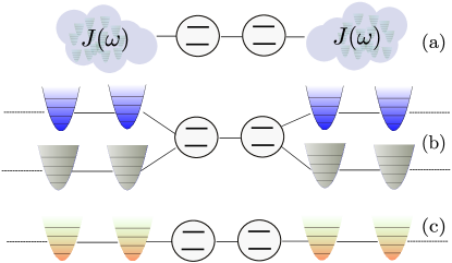
Figure 5: Comparison with the chain mapping of de Vega and Bañuls (2015). (a) Dimeric system subject to local environmental interaction. (b) The resulting chain-mapping with the double-chain approach. (c) The resulting chain mapping with T-TEDOPA; note that self-adjoint interaction operators are assumed, to halve the number of chains involved.

It is clear that the tensors associated to the two system sites by the double-chain approach have rank 4 whereas with T-TEDOPA they have rank 3. A two-site update of nearest neighbor tensors, say the $i$-th and the $j$-th with rank $r_{i}$ and $r_{j}$, requires the contraction of the two involved tensors into a single tensor. This operation produces a new tensor of rank equal $r_{i}+r_{j}-2$, which is then reshaped into a $m\times n$ matrix, where $n$ and $m$ depend on the physical and bond dimensions of the tensors. An operator is then applied to this matrix and the resulting matrix is suitably decomposed into two tensors. An essential step of this procedure is the already mentioned SVD of the $m\times n$ matrix, which, if $n\leq m$, has complexity $O(m\cdot n^{2})$. If we consider, for the sake of simplicity, the same dimension $\chi$ for all the tensor network bonds, it turns out that the complexity of of the two site update of the tensor corresponding to the dimers is $(2\chi)\cdot(2\chi)^{2}=2^{3}\cdot\chi^{3}$ for the T-SD configuration, and $(2\chi^{2})\cdot(2\chi^{2})^{2}=2^{3}\cdot\chi^{6}$ for the double-chain one.

It is clear that, even though the increased complexity of the local updates concerns only those updates that involve the TLSs, T-TEDOPA provides a dramatic improvement of the overall simulation time. Just to give an example, if the bond dimension is set to $\chi=50$, as it typically needs to be in the case of strong TLS-TLS or TLS-environment coupling, a single two-site update of the dimer would require $10^{6}$ operations with T-TEDOPA and $10^{11}$ operations with the double-chain method.

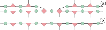
Figure 6: The tensor structure corresponding to (a) the double-chain approach, (b) T-TEDOPA, with graphical conventions as explained in the text.

.7 Hierarchical equations of motion

In Fig.2(b) in the main manuscript, we provide HEOM results for a comparison with T-TEDOPA for structured $J_{W}(\omega)$ and less-structured $J_{W}^{\prime}(\omega)$ spectral densities at $300\,{\rm K}$. The parameters of the HEOM simulations are determined by the multi-exponential fitting of the two-time correlation function Tanimura and Kubo (1989); Tanimura (2006); Lim et al. (2018a)

$$S(t) =\int_{0}^{+\infty}d\omega\ J(\omega)\left[e^{-i\omega t}(1+n_{\omega}(\beta))+e^{i\omega t}n_{\omega}(\beta)\right]$$

$$\approx\sum_{k=1}^{X/2}(A_{k}e^{(i\Omega_{k}-\Gamma_{k})t}+B_{k}e^{(-i\Omega_{k}-\Gamma_{k})t}),$$ (26)

where $A_{k}$ and $B_{k}$ are independent, complex-valued amplitudes, while $\Omega_{k}$ and $\Gamma_{k}$ are real-valued frequencies and damping rates of the exponential terms.

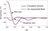
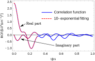
Figure 7: Two-time correlation functions at $T=300\,{\rm K}$. (a) For the less-structured $J_{W}^{\prime}(\omega)$, the correlation function is fitted by 10 exponentials up to $1\,{\rm ps}$. (b) For the structured $J_{W}(\omega)$, including additional three Lorentzian peaks, the correlation function becomes more oscillatory than (a) with additional multiple frequency components. To maintain the fitting quality with the same number of exponentials, the fitting is performed up to $0.3\,{\rm ps}$, which determines the simulation time of HEOM (see Fig.2(b) in the main manuscript).

We note that the number of exponentials is one of the dominant factors determining the HEOM simulation cost. In Fig.7(a), the two-time correlation function of the less-structured spectral density $J_{W}^{\prime}(\omega)$ is shown, which is fitted by a sum of 10 exponentials ($X=10$). The difference between target $S(t)$ and fitting function is minimized in such a way that the difference is more than two orders of magnitude smaller than the amplitude of the target function $S(t)$ up to $1\,{\rm ps}$. On the other hand, Fig.7(b) shows the case of the structured spectral density $J_{W}(\omega)$ with additional three Lorentzian peaks included, where the fitting is performed only up to $0.3\,{\rm ps}$, so that the target function $S(t)$ can be fitted by the same number of exponentials ($X=10$). This means that the optimized fitting parameters enable one to perform reliable HEOM simulations only up to $0.3\,{\rm ps}$. We note that at longer times, the correlation function starts to show additional frequency components, for instance when Fourier-transformed, not due to the ringing artifacts induced by a finite time window, but due to the presence of multiple modes in $J_{W}(\omega)$. This requires one to introduce additional exponential terms to maintain the fitting quality, which increases the HEOM simulation cost significantly. For both spectral densities, the number of auxiliary operators is increased until the system dynamics shows convergence, which is achieved at tier 14.

References

- Carmichael (1993) H. Carmichael, An Open Systems Approach to Quantum Optics (Springer-Verlag, Berlin, 1993).
- Breuer and Petruccione (2002) H.-P. Breuer and F. Petruccione, The Theroy of Open Quantum Systems (Oxford University Press, Oxford, 2002).
- Gardiner and Zoller (2004) C. W. Gardiner and P. Zoller, Quantum Noise: a Handbook of Markovian and non-Markovian Quantum Stochastic Methods with Applications (Springer, Berlin, 2004).
- Rivas and Huelga (2012) A. Rivas and S. F. Huelga, Open Quantum Systems (Springer, New York, 2012).
- Huelga and Plenio (2013) S. F. Huelga and M. B. Plenio, Contemp. Phys. 54, 181 (2013).
- Rivas et al. (2014) A. Rivas, S. F. Huelga, and M. B. Plenio, Rep. Prog. Phys 77, 094001 (2014).
- Breuer et al. (2016) H.-P. Breuer, E.-M. Laine, J. Piilo, and B. Vacchini, Rev. Mod. Phys. 88, 021002 (2016).
- de Vega and Alonso (2017) I. de Vega and D. Alonso, Rev. Mod. Phys 89, 015001 (2017).
- Luczka (1990) J. Luczka, Physica A 167, 919 (1990).
- Hu et al. (1992) B. L. Hu, J. P. Paz, and Y. Zhang, Phys. Rev. D 45, 2843 (1992).
- Garraway (1997) B. M. Garraway, Phys. Rev. A 55, 2290 (1997).
- Fisher and Breuer (2007) J. Fischer and H.-P. Breuer, Phys. Rev. A 76, 052119 (2007).
- Smirne and Vacchini (2010) A. Smirne and B. Vacchini, Phys. Rev. A 82, 022110 (2010).
- Diósi and Ferialdi (2014) L. Diósi and L. Ferialdi, Phys. Rev. Lett. 113, 200403 (2014).
- Ferialdi (2016) L. Ferialdi, Phys. Rev. Lett. 116, 120402 (2016).
- Prior et al. (2010) J. Prior, A. W. Chin, S. F. Huelga, and M. B. Plenio, Phys. Rev. Lett. 105, 050404 (2010).
- Chin et al. (2010) A. W. Chin, A. Rivas, S. F. Huelga, and M. B. Plenio, J. Math. Phys. 51, 092109 (2010).
- Woods et al. (2015) M. P. Woods, M. Cramer, and M. B. Plenio, Phys. Rev. Lett. 115, 130401 (2015).
- Prior et al. (2013) J. Prior, I. de Vega, A. W. Chin, S. F. Huelga, and M. B. Plenio, Phys. Rev. A 87, 013428 (2013).
- Chin et al. (2013) A. W. Chin, J. Prior, R. Rosenbach, F. Caycedo-Soler, S. F. Huelga, and M. B. Plenio, Nat. Phys. 9, 113 (2013).
- Hughes et al. (2009) K. Hughes, C. Christ, and I. Burghardt, J. Chem. Phys. 131, 024109 (2009).
- Martinazzo et al. (2011) R. Martinazzo, B. Vacchini, K. Hughes, and I. Burghardt, J. Chem. Phys. 134, 011101 (2011).
- Woods et al. (2014) M. P. Woods, R. Groux, A. W. Chin, S. F. Huelga, and M. B. Plenio, J. Math. Phys. 55, 032101 (2014).
- Ferialdi and Dürr (2015) L. Ferialdi and D. Dürr, Phys. Rev. A 91, 042130 (2015).
- de Vega et al. (2015) I. de Vega, U. Schollwöck, and F. A. Wolf, Phys. Rev. B 92, 155126 (2015).
- White (1992) S. R. White, Phys. Rev. Lett. 69, 2863 (1992).
- Tanimura and Kubo (1989) Y. Tanimura and R. Kubo, J. Phys. Soc. Jpn. 58, 101 (1989).
- Ishizaki and Fleming (1999) A. Ishizaki and G. R. Fleming, J. Chem. Phys. 130, 234111 (1999).
- Tanimura (2006) Y. Tanimura, J. Phys. Soc. Jpn. 75, 082001 (2006).
- Feynman (1948) R. P. Feynman, Rev. Mod. Phys. 20, 367 (1948).
- Makri (1992) N. Makri, Chem. Phys. Lett. 193, 435 (1992).
- Nalbach et al. (2010) P. Nalbach, J. Eckel, and M. Thorwart, New J. Phys. 12, 065043 (2010).
- Diósi et al. (1998) L. Diósi, N. Gisin, and W. T. Strunz, Phys. Rev. A 58, 1699 (1998).
- Yu (2004) T. Yu, Phys. Rev. A 69, 062107 (2004).
- Blasone et al. (2011) M. Blasone, P. Jizba, and G. Vitiello, Quantum Field Theory and its Macroscopic Manifestations: Boson Condensations, Ordered Patterns and Topological Defects (World Scientific, Singapore, 2011).
- de Vega and Bañuls (2015) I. de Vega and M.-C. Bañuls, Phys. Rev. A 92, 052116 (2015).
- Gautschi (1994) W. Gautschi, ACM Trans. Math. Softw. 20, 21 (1994).
- Leggett et al. (1987a) A. J. Leggett, S. Chakravarty, A. T. Dorsey, M. P. A. Fisher, A. Garg, and W. Zwerger, Rev. Mod. Phys. 59, 1 (1987a).
- Feynman and Vernon (1963) R. P. Feynman and F. L. Vernon, Ann. Phys. 24, 118 (1963).
- van Kampen (1974) N. G. van Kampen, Physica 74, 215 (1974).
- Gasbarri and Ferialdi (2018) G. Gasbarri and L. Ferialdi, Phys. Rev. A 97, 022114 (2018).
- Tamascelli et al. (2018) D. Tamascelli, A. Smirne, S. F. Huelga, and M. B. Plenio, Phys. Rev. Lett. 120, 030402 (2018).
- May and Kühn (2004) V. May and P. Kühn, Charge and Energy Transfer Dynamics in Molecular Systems (Wiley-VCH, Weinheim, 2004).
- (44) See Supplemental Material, which includes Refs. Schollwöck (2011); Rosnik and C. (2015); Lim et al. (2018a).
- Tamascelli et al. (2015) D. Tamascelli, R. Rosenbach, and M. B. Plenio, Phys. Rev. E 91, 063306 (2015).
- Kohn et al. (2018a) L. Kohn, F. Tschirsich, M. Keck, M. B. Plenio, D. Tamascelli, and S. Montangero, Phys. Rev. E 97, 013301 (2018a).
- Gautschi (2004) W. Gautschi, Orthogonal polynomials Computation and Approximation (Oxford Science Publications, Oxford, 2004).
- White and Feiguin (2004) S. R. White and A. E. Feiguin, Phys. Rev. Lett. 93, 076401 (2004).
- Rommer and Östlund (1997) S. Rommer and S. Östlund, Phys. Rev. B 55, 2164 (1997).
- Vidal (2003) G. Vidal, Phys. Rev. Lett. 91, 147902 (2003).
- Vidal (2004) G. Vidal, Phys. Rev. Lett. 93, 040502 (2004).
- Zwolak and Vidal (2004) M. Zwolak and G. Vidal, Phys. Rev. Lett. 93, 207205 (2004).
- Chandrasekaran et al. (2015) S. Chandrasekaran, Aghtar, A. Valleau, M. S. Aspuru-Guzik, and U. Kleinekathöfer, J. Phys. Chem. B 119, 9995 (2015).
- Olbrich et al. (2011) C. Olbrich, J. Strümpfer, K. Schulten, and U. Kleinekathöfer, J. Phys. Chem. Lett. 2, 1771 (2011).
- Renger et al. (2011) G. Renger, J. Pieper, C. Theiss, I. Trostmann, H. Paulsen, T. Renger, H. Eichler, and F.-J. Schmitt, J. Plant Physiol. 168, 1462 (2011).
- Alster et al. (2014) J. Alster, H. Lokstein, J. Dostál, A. Uchida, and D. Zigmantas, J. Phys. Chem. B 118, 3524 (2014).
- Vinjanampathy and Anders (2016) S. Vinjanampathy and J. Anders, Contemp. Phys. 57, 545 (2016).
- Bassi et al. (2013) A. Bassi, K. Lochan, S. Satin, T. P. Singh, and H. Ulbricht, Rev. Mod. Phys. 85, 471 (2013).
- Arndt and Hornberger (2014) M. Arndt and K. Hornberger, Nat. Phys. 10, 271 (2014).
- Cerrillo and Cao (2013) J. Cerrillo and J. Cao, Phys. Rev. Lett. 112, 110401 (2013).
- Rosenbach et al. (2016) R. Rosenbach, J. Cerrillo, S. F. Huelga, J. Cao, and M. B. Plenio, New J. Phys 18, 023035 (2016).
- Schollwöck (2011) U. Schollwöck, Ann. Phys. 326, 96 (2011).
- Rosnik and C. (2015) A. M. Rosnik and C. C., J. Chem. Theory Comput. 11, 5826 (2015).
- Lim et al. (2018a) J. Lim, C. M. Bösen, A. D. Somoza, C. P. Koch, M. B. Plenio, and S. F. Huelga, arXiv:1812.11537 (2018a).
- Kohn et al. (2018) L. Kohn, F. Tschirsich, M. Keck, M. B. Plenio, D. Tamascelli, and S. Montangero, Phys. Rev. E 97, 013301 (2018).
- (66) https://software.intel.com/en-us/intel mkl, .
- (67) https://www.openmp.org, .
- (68) https://www.mpi forum.org, .