High-resolution charge exchange spectra with L-shell nickel show striking differences from models

Abstract

We present the first high-resolution laboratory spectra of X-ray emission following L-shell charge exchange between nickel ions and neutral H₂ and He. We employ the commonly-used charge exchange models found in xspec and spex, acx and spex-cx, to simulate our experimental results. We show that significant differences between data and models exist in both line energies and strengths. In particular, we find that configuration mixing may play an important role in generating lines from core-excited states, and may be improperly treated in models. Our results indicate that if applied to astrophysical data, these models may lead to incorrect assumptions of the physical and chemical parameters of the region of interest.

1 Introduction

Charge exchange (CX) is the radiationless transfer of one or more electrons from a neutral atom or molecule to an excited state of a highly charged ion and the subsequent radiative de-excitation, and results in characteristic X-rays. CX has been found to be an important mechanism for spectral line formation in the solar system: solar wind CX is observed around comets (Lisse et al., 1996; Cravens, 1997), planetary exospheres, including our own (Dennerl et al., 2012), and it is a significant contributor to the soft X-ray background (Galeazzi et al., 2014). CX has also been postulated to occur astrophysically, in supernova remnants (Cumbee et al., 2014; Roberts et al., 2015), clusters of galaxies (Walker et al., 2015; Aharonian et al., 2017b), stellar winds (Pollock, 2007), and galactic winds (Tsuru et al., 2007).

Most observational and modeling efforts for CX have concentrated on K-shell ions. However, L-shell ions make up a non-negligible abundance fraction in a wide variety of X-ray sources, such as in Jupiter’s polar regions (Gladstone et al., 2002), and the solar wind (Schwadron & Cravens, 2000). In particular, L-shell Ni ions, though less cosmically abundant than Fe, have been identified in spectra of stellar coronae (Behar et al., 2001; Güdel & Nazé, 2009; Peretz et al., 2015) as well as in high-resolution spectra of the Sun (Phillips et al., 1982). As high-resolution spectral measurements become more routine, it will become increasingly important to understand the behavior of Ni L-shell lines compared to neighboring L-shell Fe lines in order to properly interpret spectral line diagnostics.

Because of the significance of CX in astrophysics, including its ability to quickly lower the charge state of a plasma and/or significantly alter its assumed chemical abundance, CX models are becoming more readily available. For example, acx (Smith et al., 2014) and spex-cx (Gu et al., 2016), available in the xspec and spex spectral modeling packages, respectively, have become popular tools to test for the presence of CX or explain anomalous X-ray emission in astrophysical spectra. We rely on the accuracy of these and other models and the atomic databases at their cores to perform and understand our scientific analyses. However, recent results have shown that certain comparisons across models may yield dramatically differing results (Aharonian et al., 2017a). For the case of CX, experimental data are often in conflict with models, even for K-shell ions (e.g., Beiersdorfer et al. (2000a, 2003a); Wargelin et al. (2005); Otranto et al. (2007); Leutenegger et al. (2010)). The situation is worse for CX onto L-shell ions due to their more complex atomic structure: few experimental spectra of L-shell CX exist, especially at high resolution (e.g., Crandall et al. (1979); Dijkkamp et al. (1985); Soejima et al. (1992); Folkerts et al. (1995); Lubinski et al. (2000, 2001); Beiersdorfer et al. (2000b); Tawara et al. (2002, 2003); Frankel et al. (2009)), and results from comparisons of these experiments to theoretical models, ranging from classical to quantum mechanical, are mixed, but tend towards agreeing at high collision energies and showing significant discrepancies at the low collision energies relevant to astrophysics (Soejima et al., 1992; Lubinski et al., 2000, 2001).

By performing laboratory experiments of CX between various ion and neutral species, we can learn more about the detailed atomic physics of CX and assess the accuracy and limitations of our models, determining at the atomic level where any uncertainties may exist. In this paper, we present recent measurements of CX between Ni¹⁹⁺ and He and H₂ with an Electron Beam Ion Trap (EBIT) and an X-ray microcalorimeter, and compare our experimental results to spectra produced by spex-cx and acx. We show that there are disconcerting differences between the experimental and model spectra across the L-shell Ni energy band that may stem from inconsistencies across or inaccuracies in the atomic databases.

2 Experimental Method and Line Identification

For our experiments, we used the EBIT-I electron beam ion trap at the Lawrence Livermore National Laboratory (LLNL) (Beiersdorfer et al., 2003b) and measured the spectra with the EBIT Calorimeter Spectrometer (ECS) (Porter et al., 2008). The general experimental method is described in Betancourt-Martinez et al. (2014). In brief, we create and trap our ion of interest with a tunable electron beam (a stage called direct excitation, or DE), then turn off the beam and magnetically confine the ions while we inject our neutral species, allowing CX to occur. The injection of the ion and neutral species is continuous. The ions are then dumped and the cycle is repeated, often for several hours to days to collect sufficient counts. For the experiments presented here, the length of the DE and CX phases in our analyses were approximately 0.2 and 0.3 seconds, respectively, for a total cycle time of $\sim$0.5 seconds. Nickel was supplied by sublimation of nickelocene (C₁₀H₁₀Ni) which flowed directly into the EBIT trap region. We tuned the electron beam energy to breed mostly F-like Ni (Ni¹⁹⁺), which leads to Ne-like (Ni¹⁸⁺) following single electron capture (SEC) in CX. Ne-like Ni was also present during charge breeding. This was necessary in order to avoid creating O-like, thus F-like following CX, which has several spectral lines within the Ne-like band. We injected neutral He and H₂ directly into the trap via a ballistic gas injector. Typical thermal energies of trapped ions in the EBIT are $\sim$10 eV amu^-1 ($\sim$50 km s^-1) Beiersdorfer et al. (1995, 1996). This is the approximate collision energy/velocity at which CX occurs in our experiments.

The ECS is a silicon-thermistor X-ray microcalorimeter which is described in detail in Porter et al. (2008). It has a 30-pixel array of silicon-doped thermistors which are divided into a mid- and a high-energy array. The experiments discussed here made use of 14 pixels in the mid-band array. These have an energy resolution of $\sim$4.5 eV at 6 keV and an absorber quantum efficiency across the Ni L-shell energy band of nearly unity (Porter et al., 2008). There are four aluminized polyimide infrared/optical blocking filters in the optical path of the ECS, as described in Betancourt-Martinez et al. (2014). In addition, during the experiments we checked for the presence of background contaminants that might have frozen onto one or more of the filters, such as nitrogen or water ice, which reduces the X-ray transmission. The total transmission for the experiments presented here varies smoothly in our band of interest from 0.71 at 880 eV to 0.92 at 1499 eV. The energy scale was calibrated for each pixel using X-ray emission from H- and He-like ions of O, Ne, S, and Ar, and is accurate to within 0.5 eV.

The data are time-tagged and phase-folded on the EBIT-I cycle time. For the analysis presented here, we used CX data with phase times $\geq$2 ms after the electron beam was turned off. This allows the metastable $1s^{2}_{1/2}2s^{2}_{1/2}2p_{1/2}2p^{4}_{3/2}(J=1/2)$ state of Ni¹⁹⁺, which has a lifetime of $\sim$20 $\mu$s, to relax to $1s^{2}_{1/2}2s^{2}_{1/2}2p_{1/2}^{2}2p^{3}_{3/2}(J=3/2)$. We measured the spectrum and count rate that resulted from CX with background gases in the trap by ceasing injection of our desired neutrals, and we subtracted the background spectrum. We performed these background measurements periodically during the experimental campaign period, at the beginning of the day, after the trap was pumped out overnight.

To identify the significant spectral lines present in our CX spectra, we used the energy scale and line identifications from the DE spectrum. We then compared the measured line centroids to calculations with the Flexible Atomic Code (fac) version 1.1.3 (Gu et al., 2008) and measurements of L-shell Ni lines with a high-resolution grating spectrometer from Gu et al. (2007). In our fac calculation, we corrected the ground state ionization energies of Ne-like Ni according to Scofield (private communication), and the $3\rightarrow 2$ transition energies to match those in Gu et al. (2007). The error on our calculated transition energies is dominated by ground state ionization energies, which we estimate to be $\sim$1 eV. These line identifications are presented in Table LABEL:table:lineID. In some cases, one line may be a combination of several transitions presented. Some F-like Ni lines are also included in our identifications; these would be present following SEC in CX with an O-like ion. They should only be a minor contribution to the spectrum due to the fact that the O-like $2p_{1/2}2p_{3/2}^{2}3d_{5/2}(J=3)\rightarrow 2p_{3/2}^{2}(J=2)$ transition at $\sim$1096 eV, which should be the strongest one in the O-like series in DE (Gu et al., 2007), is not significant in our spectra.

The spectra shown in the following sections are background-subtracted but are not corrected for filter attenuation; the models are adjusted for this attenuation to match the experimental spectra.

3 Key Spectral Features

Figure 1 presents our measured CX spectra with both neutral partners, as well as a DE spectrum following collisional excitation. The strongest line in both Ni¹⁹⁺+H₂ and Ni¹⁹⁺+He CX spectra is a blend of the M2 ($2p_{3/2}^{3}3s_{1/2}(J=2)\rightarrow 2p_{3/2}^{4}(J=0)$) and 3G ($2p_{3/2}^{3}3s_{1/2}(J=1)\rightarrow 2p_{3/2}^{4}(J=0)$) lines. This is a stark difference from the DE spectrum, which at the $\sim$4.5 eV resolution of the ECS, has four prominent lines from $n=3\rightarrow 2$ transitions: M2/3G, 3F ($2p_{1/2}^{1}3s_{1/2}^{1}(J=1)\rightarrow 2p_{3/2}^{4}(J=0)$), 3D ($2p_{3/2}^{3}3d_{5/2}^{1}(J=1)\rightarrow 2p_{3/2}^{4}(J=0)$), and 3C ($2p_{1/2}^{1}3d_{3/2}^{3}(J=1)\rightarrow 2p_{3/2}^{4}(J=0)$). The relative enhancement of the M2/3G lines and suppression of the 3F, 3D, and 3C lines may be seen as strongly diagnostic of the presence of CX.

Line label as shown in the figures in this work, following the notation of Parkinson (1973); Loulergue & Nussbaumer (1975), or lowercase alphabetic label if the observed line may result from a blend of transitions or is unidentified. An asterisk indicates a line that results from core excitation.

Line identification of a possible component of a blended line. Labels follow the notation of Parkinson (1973); Loulergue & Nussbaumer (1975), and an asterisk indicates a line that results from core excitation. A dagger indicates an unidentified line.

The energy of the peak of the line measured in our DE spectrum.

Line energy calculated in fac.

Line energy in Gu et al. (2007).

Line energy (converted from observed wavelength) from the NIST atomic spectra lines database.

Upper state for the transition presented. The lower state for all Ni¹⁸⁺ ions is $2p_{3/2}^{4}(J=0)$, and the lower state for the Ni¹⁹⁺ transitions here is $2p_{3/2}^{3}(J=3/2)$.

Table 1: Line identifications for the strongest lines observed in our measured CX spectra

Labela	Secondary Labelb	DE (eV)c	FAC (eV)d	Gu (eV)e	NIST (eV)f	Upper Stateg
M2		882	880.753	880.827	880.827	$2p_{3/2}^{3}3s_{1/2}(J=2)$
3G			882.888	882.96	882.960	$2p_{3/2}^{3}3s_{1/2}(J=1)$
3F*		900	899.807	899.877	899.877	$2p_{1/2}3s_{1/2}(J=1)$
E2L		919	920.037	918.542		$2p_{3/2}^{3}3p_{1/2}(J=2)$
a		925	926.041			$2p_{3/2}^{3}3p_{3/2}^{3}(J=2)$
F4		932		931.586		$2p_{3/2}^{2}3s_{1/2}(J=5/2)$
E2U*		941	942.002	940.346		$2p_{1/2}3p_{3/2}(J=2)$
3E		967	969.255	967.947	967.796	$2p_{3/2}^{3}3d_{3/2}(J=1)$
3D		980	979.487	979.571	979.725	$2p_{3/2}^{3}3d_{5/2}(J=1)$
3C*		997	997.139	997.218	997.138	$2p_{1/2}3d_{3/2}(J=1)$
b	F14	1023		1023.475	1023.729	$2p_{3/2}^{2}3d_{5/2}(J=5/2)$
	F15			1023.475	1022.210	$2p_{3/2}^{2}3d_{5/2}(J=3/2)$
3B*		1070	1073.451		1069.006	$2s_{1/2}3p_{1/2}(J=1)$
3A*		1074	1079.017	1074.844	1074.565	$2s_{1/2}3p_{3/2}(J=1)$
4G		1188	1190.006		1188.479	$2p_{3/2}^{3}4s_{1/2}(J=1)$
4F*		1207	1207.353		1205.816	$2p_{1/2}4s_{1/2}(J=1)$
4D		1226	1228.023	1226.207	1226.450	$2p_{3/2}^{3}4d_{5/2}(J=1)$
4C*		1243	1244.359		1242.799	$2p_{1/2}4d_{3/2}^{3}(J=1)$
5G		1322	1322.537			$2p_{3/2}^{3}5s_{1/2}(J=1)$
c	5E	1340	1338.760		1338.739	$2p_{3/2}^{3}5d_{3/2}(J=1)$
	5F*		1340.036			$2p_{1/2}5s_{1/2}(J=1)$
	5D		1341.376		1339.897	$2p_{3/2}^{3}5d_{5/2}(J=1)$
d	4B*	1356	1356.458		1354.682	$2s_{1/2}4p_{1/2}(J=1)$
	5C*		1358.142			$2p_{1/2}5d_{3/2}(J=1)$
	4A*		1358.583		1356.609	$2s_{1/2}4p_{3/2}(J=1)$
6G		1390	1391.931			$2p_{3/2}^{3}6s_{1/2}(J=1)$
6D		1401	1402.566		1401.221	$2p_{3/2}^{3}6d_{5/2}(J=1)$
e	$\dagger$	1423
7G		1432	1432.827			$2p_{3/2}^{3}7s_{1/2}(J=1)$
7D		1438	1439.425		1439.448	$2p_{3/2}^{3}7d_{5/2}(J=1)$
f	8E	1462	1462.704		1460.988	$2p_{3/2}^{3}8d_{3/2}(J=1)$
	8D		1463.288			$2p_{3/2}^{3}8d_{5/2}(J=1)$
g	9G	1479	1476.579			$2p_{3/2}^{3}9s_{1/2}(J=1)$
	8F*		1476.658			$2p_{1/2}8s_{1/2}(J=1)$
	9D		1479.618			$2p_{3/2}^{3}9d_{5/2}(J=1)$
	8C*		1480.824			$2p_{1/2}8d_{3/2}(J=1)$
	5B*		1481.395			$2s_{1/2}5p_{1/2}(J=1)$
	5A*		1482.437			$2s_{1/2}5p_{3/2}(J=1)$
h	10G	1490	1489.084			$2p_{3/2}^{3}10s_{1/2}(J=1)$
	10D		1491.282			$2p_{3/2}^{3}10d_{5/2}(J=1)$
i	9C*	1499	1497.226			$2p_{1/2}9d_{3/2}(J=1)$
	11G		1498.262			$2p_{3/2}^{3}11s_{1/2}(J=1)$
	11D		1499.902			$2p_{3/2}^{3}11d_{5/2}(J=1)$

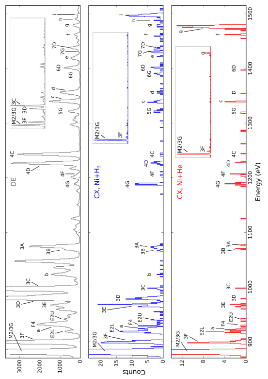
Figure 1: Magnified spectra of Ni¹⁹⁺ and Ni¹⁸⁺ created in DE (top) and CX between Ni¹⁹⁺+H₂ (middle) and Ni¹⁹⁺+He (bottom). The full L-shell spectra are shown in the insets. Significant CX lines are identified by labels that correspond to entries in Table LABEL:table:lineID; lines that may result from blends are labeled alphabetically. The M2/3G lines dominate the CX spectra, while the 3F, 3D, and 3C lines are suppressed compared to DE. We also observe a difference in $n$_max $\rightarrow 2$ transitions from 1450 eV–1500 eV between the Ni¹⁹⁺+H₂ and the Ni¹⁹⁺+He spectra, which likely stems from the differing ionization potentials of the two neutrals. In this and all following figures, the data have been background-subtracted but have not been adjusted for filter transmission. The total number of counts in the M2/3G lines in the DE, Ni¹⁹⁺+H₂, and Ni¹⁹⁺+He spectra are $\sim$133000, $\sim$1750, and $\sim$600, respectively.

Another key diagnostic of CX stems from the fact that CX typically leads to electron capture into a high-$n$ state (Janev, 1983). The $l$ capture state, while harder to predict, has been shown to vary with the collision energy: at high collision energies, the states are populated statistically, favoring higher angular momentum states (Janev & Winter, 1985), and at the low collision energies produced with the EBIT, lower angular momentum states are favored (Ryufuku & Watanabe, 1979; Beiersdorfer et al., 2000a). This leads to a strong $11s$ or $11d\rightarrow 2p$ transition observed in the Ni¹⁹⁺+H₂ spectrum and $8d$ or $9d\rightarrow 2p$ transition in the Ni¹⁹⁺+He spectrum. The decrease in the $n$_max state between experiments with H₂ and He likely stems from their differing first ionization potentials ($\sim$15.4 eV and $\sim$24.6 eV, respectively).

We also observe the presence of lines that result from core-excited states: for example, an electron hole in $2s_{1/2}$ being filled by either a $3p_{3/2}$ or $3p_{1/2}$ electron (to create the 3A and 3B lines, respectively), or a hole in $2p_{1/2}$ being filled by a $3s_{1/2}$ electron (to create the 3F line). This is surprising under the naive assumption that the parent F-like ion would be in the ground state with no core excitation, $1s_{1/2}^{2}2s_{1/2}^{2}2p_{1/2}^{2}2p_{3/2}^{3}$, and that CX would not influence the core configuration. However, previous experiments and subsequent modeling of CX with higher-Z ions (e.g. Tawara et al. (2002); Schuch et al. (2000)) have shown that electron-electron interactions (i.e., configuration mixing) during or after electron capture can lead to core excited states.

To further investigate this effect for our ion of interest, we performed fac structure calculations of Ni¹⁸⁺ with one excited electron using two different mixing schemes: mixing only between levels with the excited electron in the same $n$-level, and mixing between all levels. A comparison of cascade spectra resulting from capture into a single excited state is presented in Figure 2. We found that lines from upper levels with core excited states are more likely to occur if all levels are allowed to mix, and in general, the two resulting spectra can be dramatically different. This reinforces the results from Tawara et al. (2002) and Schuch et al. (2000) that mixing is likely the main mechanism for generating core excitation following CX. In addition, this indicates that how mixing is treated in cascades can greatly impact the resulting spectrum, and should be considered carefully. With an adequate understanding of the mixing configurations and subsequent decay schemes, core excited lines following CX may be an additional diagnostic of the quantum state of the captured electron.

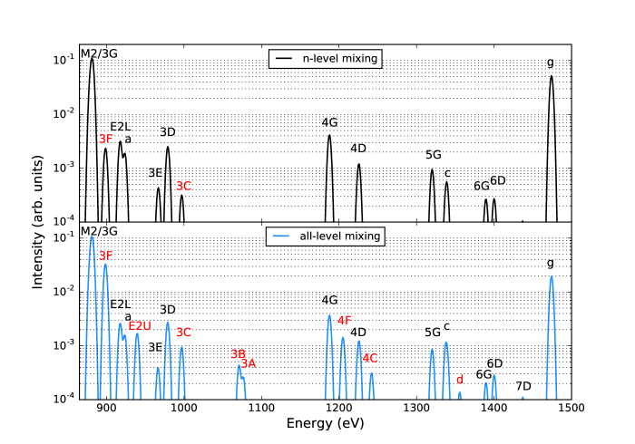
Figure 2: Simulated spectra resulting from cascades following electron capture into $2p_{3/2}^{3}9s_{1/2}(J=1)$ (creating Ne-like Ni), via fac structure calculations, with two different mixing schemes. Top: only levels with like $n$ for the excited electron mix. Bottom: all levels mix. Line labels correspond to entries in Table LABEL:table:lineID, and transitions resulting from core excited states are highlighted in red. For this capture state, allowing all levels to mix is more likely to generate core excited states, and in general, the two mixing schemes generate distinct spectra.

4 Spectral Models

We used spex-cx version 3.0 and acx version 1.0 to simulate spectra for interactions between Ni¹⁹⁺+H (spex-cx, acx) and Ni¹⁹⁺+He (acx only) and to compare with our experimental spectra. Although in some cases, the models and data involve differing neutrals, some have similar ionization potentials (IP, 15.4 eV for H₂ and 13.6 eV for H, though a slightly higher IP of 24.6 eV for He), and all have at most two electrons available for capture. We believe that our most significant findings do not depend on the neutral partner, as the main effect we expect is a decrease in $n$_max with increasing IP (Janev & Winter, 1985). However, multi-electron capture (MEC) must still be considered in the H₂ and He cases, and intrinsic differences in the state-selective cross sections between the various neutrals may also be present.

To simulate CX in acx, we used the acxion model and convolved the resulting spectrum with a Gaussian line profile to match the instrumental response of the ECS. We set the parent ion to be Ni¹⁹⁺, and considered CX with either pure H or pure He by adjusting the fracHe0 parameter. We used two different $l$-distributions for the captured electrons by varying the model parameter: model “8,” which is the default model used in acx and which assumes a separable $l$-distribution, and model “15,” which uses a Landau-Zener weighting function for the total $L$-distribution. Model 15 was chosen because Landau-Zener methods are known for being most applicable to low-energy CX collisions such as those in EBITs (Janev et al., 1985).

For the spex-cx model, we used the lowest allowable collision velocity of 50 km s^-1, the approximate ionization temperature of 500 eV, and zeroed out the abundance of all ions except Ni. While this does not exactly describe our system—in particular, in the mode in which we operated the electron beam, it does not have a thermal Maxwellian electron distribution—500 eV yielded the closest match to our spectra upon visual inspection after stepping through several values, and the lowest c-statistic after performing a model fit to the data. We left the weight parameter at the default value, which picks the most appropriate $l$-distribution based on the velocity. In our case, this was the Landau-Zener $l$-distribution. We convolved the model spectrum with a Gaussian line profile. spex-cx does not have the ability to consider neutral partners other than H.

5 Model Comparison Results

Figures 3 and 4 show the results of the comparisons between models and data, in some cases cross-comparing spectra assuming different neutrals. In general, these comparisons show that although some lines are well approximated by the models, most lines are dramatically over- or under-predicted, and in some cases, line energies for the same atomic transition differ between the models and those identified in our data by over 10 eV.

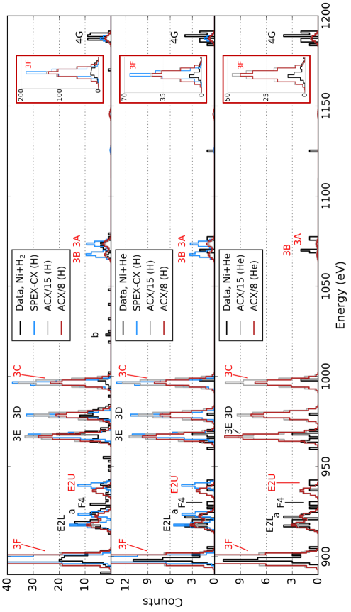
Figure 3: EBIT data compared to the spex-cx and acx models from 890–1200 eV, with the neutral used in each spectrum indicated in the legend. Lines resulting from core excited states are indicated with red labels. Model line strengths are normalized to the total number of counts in the M2/3G lines in the data being compared in each panel (not shown for scale).

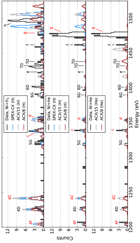
Figure 4: As in Figure 3, but from 1200–1525 eV.

An important energy regime that the models fail to correctly reproduce is near the strong high-$n\rightarrow n=2$ transition(s) between 1450–1500 eV. The canonical equation to estimate the primary $n$ capture state of the transferred electron, used in both spex-cx and acx codes for CX with L-shell Ni, is:

$$n\textsubscript{max}=q\sqrt{\frac{I_{\mathrm{H}}}{I_{\mathrm{n}}}}\left(1+\frac{q-1}{\sqrt{2q}}\right)^{-1/2},$$ (1)

where $I$_H and $I$_n are the ionization potentials of hydrogen and the neutral target, respectively, and $q$ is the ion charge (Janev & Winter, 1985).

This equation predicts $n$_max$=9.6$ for CX with atomic H. The acx models we used for CX with H thus assume 60% of electron capture into $n=10$ and 40% into $n=9$. The spex-cx model for CX with H assumes capture into $n=10$. For CX with He, Equation 1 predicts $n$_max$=7.1$, and $n$_max$=9.0$ for CX with H₂.

These model estimates clearly differ from our measurements, where there is very little capture into these $n$ levels: the primary capture state in our spectra of Ni${}^{19+}+$H₂ is $n=11$, and 8–9 for Ni${}^{19+}+$He. This highlights the approximate nature of this equation, which may cause problems when fitting spectra from celestial sources. Furthermore, transitions that involve $n>10$ are not included for any ions in acx, and for Ne-like ions in spex-cx, so it is not currently possible for the models to reproduce our results even with a more accurate $n$_max distribution (Randall Smith and Liyi Gu, private communication).

In addition, the line energies used in the acx model can differ from those from our fac calculation by a large amount. When the spectral lines in this high-$n$ region are identified according to acx versus fac, the $n$ state predicted for a given line can differ by up to $\Delta n=3$ between the two models (Adam Foster, private communication). This corresponds to a difference in $\sim$10 eV between the two models for the same atomic transition. acx also predicts a line at $\sim$1150 eV corresponding to $2s3d\rightarrow$ ground transitions; this line falls $\sim$17 eV away from where these transitions are predicted to occur from fac.

We also found that lines resulting from core-excited states were mostly over-predicted by both models. These lines are highlighted in red in Figures 3 and 4. acx and spex-cx both include mixing in their cascades (Adam Foster and Liyi Gu, private communication), but as we saw in Figure 2, the details of exactly how mixing is treated can have a large impact on the resulting spectrum. The discrepancies we observe between our data and models show that more detailed calculations of the strength of configuration mixing and levels involved should be performed, compared to experimental benchmarks, and incorporated into these models to improve their accuracy.

6 Summary

We have presented high-resolution spectra of CX between L-shell Ni and neutral H₂ and He, and identify spectral diagnostics. We find that configuration mixing is an important effect to include in CX models to generate the core excitation that we observe, as in Tawara et al. (2002); Schuch et al. (2000). We show that spex-cx and acx models do not accurately reproduce our experimental results, with disconcerting differences across the L-shell energy band. This is likely due to the approximate nature of the scaling equations used to estimate the $n$_max and $l$ distributions, limitations in the databases for high-$n$ energy levels, inaccurate line energies, and improper treatment of configuration mixing, though intrinsic differences between state-selective cross sections with H, H₂, and He may also play a role.

While the availability and relative ease of use of models such as acx and spex-cx are beneficial for encouraging the incorporation of CX into spectral analyses, these comparisons show that these models must be used with caution. If they are applied to astrophysical data, incorrect assumptions may be made about the physical and chemical parameters of the observation target, such as the neutral species present, the ion or neutral abundance, or the ion/neutral collision energy, due to potentially misleading predicted line strengths or ratios. The discrepancies we show between experiments and models presented here highlight the need for careful atomic structure calculations for L-shell ions, including both transition energies and mixing coefficients, in order to generate accurate cascades, as well as detailed state-selective cross section calculations for CX, particularly at low collision energies. It is also important to compare these values across models and against laboratory data in order to ensure that spectra from CX and other recombination processes are sufficiently accurate. These calculations and comparisons are especially critical to perform in advance of the forthcoming high-resolution spectra from future satellites such as XRISM and Athena.

References

- Aharonian et al. (2017a) Aharonian, F. A., Akamatsu, H., Akimoto, F., et al. 2017a, ArXiv e-prints, arXiv:1712.05407
- Aharonian et al. (2017b) Aharonian, F. A., Akamatsu, H., Akimoto, F., et al. 2017b, ApJ, 837, L15
- Behar et al. (2001) Behar, E., Cottam, J., & Kahn, S. M. 2001, ApJ, 548, 966
- Beiersdorfer et al. (1995) Beiersdorfer, P., Decaux, V., Elliott, S. R., Widmann, K., & Wong, K. 1995, Rev. Sci. Instr., 66, 303
- Beiersdorfer et al. (1996) Beiersdorfer, P., Osterheld, A. L., Decaux, V., & Widmann, K. 1996, Phys. Rev. Lett., 77, 5353
- Beiersdorfer et al. (2000a) Beiersdorfer, P., Olson, R. E., Brown, G. V., et al. 2000a, Phys. Rev. Lett., 85, 5090
- Beiersdorfer et al. (2000b) Beiersdorfer, P., Olson, R. E., Schweikhard, L., et al. 2000b, AIP Conf. Series, Vol. 500, AIP Conf. Series, 626–635
- Beiersdorfer et al. (2003a) Beiersdorfer, P., Boyce, K. R., Brown, G. V., et al. 2003a, Science, 300, 1558
- Beiersdorfer et al. (2003b) Beiersdorfer, P., Behar, E., Boyce, K. R., et al. 2003b, Nucl. Instrum. Methods Phys. Res. B, 205, 173
- Betancourt-Martinez et al. (2014) Betancourt-Martinez, G. L., Beiersdorfer, P., Brown, G. V., et al. 2014, Phys. Rev. A, 90, 052723
- Crandall et al. (1979) Crandall, D. H., Phaneuf, R. A., & Meyer, F. W. 1979, Phys. Rev. A, 19, 504
- Cravens (1997) Cravens, T. E. 1997, Geophys. Res. Lett., 24, 105
- Cumbee et al. (2014) Cumbee, R. S., Henley, D. B., Stancil, P. C., et al. 2014, ApJ, 787, L31
- Dennerl et al. (2012) Dennerl, K., Lisse, C. M., Bhardwaj, A., et al. 2012, Astron. Nachr., 333, 324
- Dijkkamp et al. (1985) Dijkkamp, D., Ciric, D., de Boer, A., de Heer, F. J., & Vlieg, E. 1985, J. Phys. B: At., Mol. Phys., 18, 4763
- Folkerts et al. (1995) Folkerts, L., Haque, M. A., Havener, C. C., Shimakura, N., & Kimura, M. 1995, Phys. Rev. A, 51, 3685
- Frankel et al. (2009) Frankel, M., Beiersdorfer, P., Brown, G. V., et al. 2009, ApJ, 702, 171
- Galeazzi et al. (2014) Galeazzi, M., Chiao, M., Collier, M. R., et al. 2014, Nature, 512, 171
- Gladstone et al. (2002) Gladstone, G. R., Waite, J. H., Grodent, D., et al. 2002, Nature, 415, 1000
- Gu et al. (2016) Gu, L., Kaastra, J., & Raassen, A. J. J. 2016, A&A, 588, A52
- Gu et al. (2008) Gu, M. F. 2008, Can. J. Phys., 86, 675
- Gu et al. (2007) Gu, M. F., Beiersdorfer, P., Brown, G. V., et al. 2007, ApJ, 657, 1172
- Güdel & Nazé (2009) Güdel, M., & Nazé, Y. 2009, A&A Rev., 17, 309
- Janev (1983) Janev, R. K. 1983, Phys. Scr. Volume T, 3, 208
- Janev et al. (1985) Janev, R. K., Presnyakov, L. P., & Shevelko, V. P. 1985, Physics of highly charged ions
- Janev & Winter (1985) Janev, R. K., & Winter, H. 1985, Phys. Rep., 117, 265
- Leutenegger et al. (2010) Leutenegger, M. A., Beiersdorfer, P., Brown, G. V., et al. 2010, Phys. Rev. Lett., 105, 063201
- Lisse et al. (1996) Lisse, C. M., Dennerl, K., Englhauser, J., et al. 1996, Science, 274, 205
- Loulergue & Nussbaumer (1975) Loulergue, M. & Nussbaumer, H. 1975, A&A, 45, 125
- Lubinski et al. (2000) Lubinski, G., Juhász, Z., Morgenstern, R., & Hoekstra, R. 2000, J. Phys. B: At., Mol. Phys., 33, 5275
- Lubinski et al. (2001) Lubinski, G., Juhász, Z., Morgenstern, R., & Hoekstra, R. 2001, Phys. Rev. Lett., 86, 616
- Otranto et al. (2007) Otranto, S., Olson, R. E., & Beiersdorfer, P. 2007, J. Phys.: Conf. Series, 58, 165
- Parkinson (1973) Parkinson, J. H. 1973, A&A, 24, 215
- Peretz et al. (2015) Peretz, U., Behar, E., & Drake, S. A. 2015, A&A, 577, A93
- Phillips et al. (1982) Phillips, K. J. H., Fawcett, B. C., Kent, B. J., et al. 1982, ApJ, 256, 774
- Pollock (2007) Pollock, A. M. T. 2007, A&A, 463, 1111
- Porter et al. (2008) Porter, F. S., Gygax, J., Kelley, R. L., et al. 2008, Rev. Sci. Instr., 79, 10E307
- Roberts et al. (2015) Roberts, S. R., & Wang, Q. D. 2015, MNRAS, 449, 1340
- Ryufuku & Watanabe (1979) Ryufuku, H., & Watanabe, T. 1979, Phys. Rev. A, 20, 1828
- Schuch et al. (2000) Schuch, R., Madzunkov, S., Lindroth, E., & Fry, D. 2000 Phys. Rev. Lett., 85, 26
- Schwadron & Cravens (2000) Schwadron, N. A., & Cravens, T. E. 2000, ApJ, 544, 558
- Smith et al. (2014) Smith, R. K., Foster, A. R., Edgar, R. J., & Brickhouse, N. S. 2014, ApJ, 787, 77
- Soejima et al. (1992) Soejima, K., Latimer, C. J., Okuno, K., Kobayashi, N., & Kaneko, Y. 1992, J. Phys. B: At., Mol. Phys., 25, 3009
- Tawara et al. (2002) Tawara, H., Richard, P., Safronova, U. I., et al. 2002, Phys. Rev. A, 65, 042509
- Tawara et al. (2002) Tawara, H., Richard, P., Safronova, U. I., Vasilyev, A. A., & Stockli, M. 2002, Can. J. Phys. 80, 821
- Tawara et al. (2003) Tawara, H., Takács, E., Ratliff, L. P., Gillaspy, J. D., & Tőkési, K. 2003, Nucl. Instrum. Methods Phys. Res. B, 205, 605
- Tsuru et al. (2007) Tsuru, T. G., Ozawa, M., Hyodo, Y., et al. 2007, PASJ, 59, 269
- Walker et al. (2015) Walker, S. A., Kosec, P., Fabian, A. C., & Sanders, J. S. 2015, MNRAS, 453, 2480
- Wargelin et al. (2005) Wargelin, B. J., Beiersdorfer, P., Neill, P. A., Olson, R. E., & Scofield, J. H. 2005, ApJ, 634, 687