Sym-parameterized Dynamic Inference for Mixed-Domain Image Translation
Abstract
Recent advances in image-to-image translation have led to some ways to generate multiple domain images through a single network. However, there is still a limit in creating an image of a target domain without a dataset on it. We propose a method that expands the concept of ‘multi-domain’ from data to the loss area and learns the combined characteristics of each domain to dynamically infer translations of images in mixed domains. First, we introduce Sym-parameter and its learning method for variously mixed losses while synchronizing them with input conditions. Then, we propose Sym-parameterized Generative Network (SGN) which is empirically confirmed of learning mixed characteristics of various data and losses, and translating images to any mixed-domain without ground truths, such as 30% Van Gogh and 20% Monet and 40% snowy.
1 Introduction
Recently, literature on multi-domain deep image translation has introduced many methods that learn the joint distribution of two or more domains and find transformations among them. Particularly, a single generator is able to translate images to multiple domains based on training data distributions [3, 20, 26]. However, translating style features across domains seen by the model is different from ‘creativeness’. Consider a case of generating a translated image with a style that is 20% of Van Gogh, 50% of Picasso and 30% of the original image. Since the ground truths for learning such a translation do not exist, the target distribution to approximate can not explicitly be provided for conventional deep generative networks.
If we construe that the optimum of the target style is a weighted sum of optima of the candidate styles, then the objective function can be defined by a weighted sum of objective functions of those. In this end, if the weights are set as hyper-parameters, they can be preselected and learned to generate images outside of a domain even without ground truths [5]. Even in such a case, not only a criterion on selections of the parameters is vague, but every training for cross-domain translations must also be impractically done with a unique set of weights. Therefore, it would be more efficient to dynamically control them during inferences for desired translations. We, in this paper, present a concept of sym-parameters that enable human users to control them so that influences of candidate domains on final translations can be heuristically adjusted during inferences.
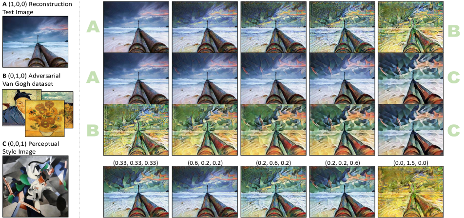
In our method, along with inputs, sym-parameters are inputted as a condition into our proposed generator network, Sym-parameterized Generative Network (SGN). And also, these sym-parameters are synchronously set as weights for the linear combination of multiple loss functions. With the proposed setting, we have verified that a single network is able to generate corresponding images of a mixed-domain based on an arbitrarily weighted combination of loss functions without direct ground truths. While an SGN utilizes multiple loss functions that conventional image-to-image translation models use (e.g. reconstruction loss, GAN (adversarial) loss, perceptual loss), the sym-parameter conditions the weights of these losses for variously purposed translations. If an SGN, as an exemplar case depicted in Figure 1, uses GAN loss for training Van Gogh style and perceptual loss for Udnie of Francis Picabia, sym-parameters allow adjusting the ratio of the styles to create correspondingly styled images. Through experiments, we found that sym-parameters conditioned within a model in the ways performed in typical conditional methods [3, 15, 30], fail to yield our intended generations. To overcome this, we additionally propose Conditional Channel Attention Module (CCAM).
To summarize, our contributions are as follows:
(1) We propose the concept of sym-parameter and its learning method that can control the weight between losses during inferences.
(2) We introduce SGN, a novel generative network that expands the concept of ‘multi-domain’ from data to the loss area using sym-parameters.
(3) Experimental results show that SGN could translate images to mixed-domain without ground truths.
2 Related work
Generative Adversarial Networks Recently, Generative Adversarial Networks (GANs) [6] have been actively adapted to many image generation tasks [1, 11, 16, 21]. GANs are typically composed of two networks: a generator and a discriminator. The discriminator is trained to distinguish the generated samples (fake samples) from the ground-truth images (real samples), while the generator learns to generate samples so that the discriminator misjudges. This training method is called adversarial training which our method uses for both the generator and the discriminator to learn the distribution of a real dataset.
Conditional Image Synthesis By conditioning concurrently with inputs, image generation methods learn conditional distribution of a domain. CVAE [24] uses conditions to assign intentions to VAEs [13]. Conditional image generation methods that are based on GANs also have been developed [2, 4, 18, 19, 20, 28], using class labels or other characteristics. Conditional GANs are also used in domain transfers [12, 25] and super-resolution [16]. While the methods from [3, 20] use discrete conditioning (either 0 or 1), our method uses continuous values for input conditioning.
Image to Image Translation While there exist generative models that generate images based on sampling (i.e. GANs, VAEs), models that generate images for given base input images are also studied. They mostly use autoencoders [14] and among them, one of the most representative and recent works is [9], which uses adversarial training with conditions. CycleGAN [29] and DiscoGAN [12] translate either style or domain of input images. Johnson et al. [10] have proposed perceptual loss in order to train feed-forward network for image style transformation. Since most of them use convolutional autoencoders with ResBlocks [7] or U-Net [22] structure, we also utilize the structure of CycleGAN [29], but additionally apply sym-parameters to image-to-image translation tasks in the form of continuous valued conditions. We also adopt the perceptual loss harmonized with the GAN loss and the reconstruction loss terms.
One generator to multiple domains Many have extended the study of image-to-image translations to multiple domains with a single generator network. IcGAN [20], StarGAN [3] and SingleGAN [26] address the problem of previously reported generative models that they are stuck with two domains, and achieve meaningful results on their extended works by using hard labels of each domain. Methods regarding image generation problems also have been proposed. ACGAN [19] uses auxiliary classifier to generate images by providing class information as a condition in the input. In different perspective, CAN [5] tries generating artworks by blending multiple domains. The method trains the generator of GAN to confuse the auxiliary classifier to judge fake samples in forms of uniform-distribution. In this study, we make a good use of conditions synchronized with loss functions not only to transfer to multiple domains, but also to mix each styles simultaneously by using expandable loss terms.
3 Proposed Method
Our goal is to learn distributions from multiple domains by varying weighted loss functions in order to dynamically translate images into a mixed-domain. In order to control mixing ratio during inferences, the corresponding conditions must be inputted and trained with the model. For such purpose, we present sym-parameters which are symmetrically set inside (as condition inputs) as well as outside (as weights of multiple loss functions) of a generator. The sym-paraemters allow transitive learning without explicit ground truth images among diverse mixtures of multiple domains and loss functions. The generator of sym-parameterized generative networks (SGN) can thus be controlled during inferences unlike conventional generators that infer strictly as optimized for a specific dataset or a particular loss function.
3.1 Sym-parameter
By trying to find not only the optimum of each candidate objective function but also the optima for various combinations of them, we desire to control the mixing weights during inferences. We propose human controllable parameters, Sym-parameters, that can replace typical hyper-parameters for weighing multiple loss functions. As the prefix “sym-” is defined in dictionaries as “with; along with; together; at the same time”, sym-parameters are fed into a model, symmetrically set as weights of the candidate loss functions and synchronized after training. If number of different loss functions, , are engaged, then the sym-parameter is defined as a -dimensional vector . The total loss of a model that takes inputs and sym-parameters is:
| (1) | ||||
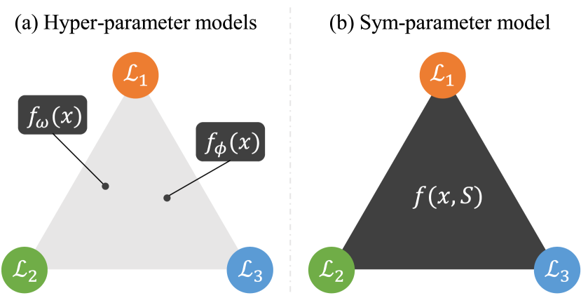
Having the total sum of sym-parameters to be 1, the total loss defined by the function and sym-parameters is a weighted sum of sub-loss functions, each of which is weighed by the corresponding element of . The conventional hyper-parameter model predicts output using the model with hyper-parameter . In this case, it is difficult to predict for , that is not used during training, because the network is not a conditional function for the hyper-parameter that was not used at training time. However, our model uses the weight of losses as input in the form , and has conditional output for as well as . Thus, it can predict for various combinations of losses that were used in training. Figure 2 depicts the concept showing the difference between a sym-parametrized model and conventional models using multiple loss functions weighted by hyper-parameters. While a new model is required for learning each combination of weights if conventional methods are used, our method allows a single model to manage various combination of weights through one learning. We, in the experiment section, verify that not only each sub-objective function is optimized but various linear sums of them also are. For example, if a neural model wants to perform both the regression and the classification tasks, the optimization is processed towards minimizing the regression loss when , the classification loss when and the weighted sum of the losses when .
Training with Dirichlet Distribution As mentioned above, a sym-parameter is represented as a vector which has the same number of dimensions as the number of loss functions. The vector’s values are randomly selected during training in order to synchronize accordingly with sym-parameterized combinations of loss functions. To do so, the sym-parameter values are sampled based on Dirichlet distribution. The probability distribution of a -dimensional vector with the sum of positively valued elements being 1, can be written as:
| (2) |
Here, is a normalization constant and represents Gamma function. When , the distribution boils down to Beta distribution. Using Dirichlet distribution allows the sum of sym-parameter values to be 1 and enables adjusting the distribution with by changing the concentration vector .
3.2 Sym-parameterized Generative Networks
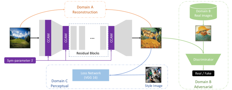
Using sym-parameters that allow inferences of various mixtures of losses, we propose sym-parametrized generative networks (SGN) that translate images to a mixed-domain. Our method is able to either generate images from latent inputs or translate styles with image inputs as long as sym-parameters are inputted along with the inputs and they define a linear combination of loss functions. Figure 3 illustrates the structure of SGN for image-to-image translation. Selection of loss functions are not necessarily limited for image generation tasks, and the following is a representative loss for a generator with reconstruction loss , adversarial loss and perceptual loss weighted by sym-parameters :
| (3) |
Here, each loss function may cope with different objective and dataset for more diverse image generations such as using two of adversarial losses one of which for Van Gogh and another for Monet style domain.
While either reconstruction loss or perceptual loss does not require to train an additional network, a discriminator must be trained along with an SGN model for the adversarial loss, and a distinct training criterion of the discriminator is needed for SGN. Because our method generates images based on linearly combined losses with sym-parametrized weights, the weight on the loss of a discriminator must be also set accordingly. Therefore, discriminator must be trained with the weight assigned on the generator loss in an adversarial manner:
| (4) |
A trained SGN can translate images with specific sym-parameters, or generate random images from random variables sampled from Dirichlet distribution defined by an input image.

3.2.1 Conditional Channel Attention Module
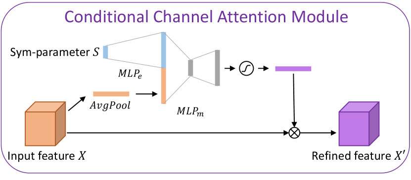
SGN takes a continuous valued sym-parameter vector along with inputs and generates images reflecting characteristics of various parts of a mixed-domain, which covers wider range of target distribution than multi-domain models do with discrete conditions. Since domain injection used in conventional conditional generators is empirically shown to be inadequate for our purpose, we propose another injection method for sym-parameterized conditionings, named Conditional Channel Attetion Module (CCAM). Inspired by SENet [8], CCAM is a channel attention model that selectively gates feature channels based on sigmoid attentiveness. CCAM also allows SGN to have a fully convolutional structure and manage various spatial sizes. CCAM’s structural details are depicted in Figure 4, and the module can be written as:
| (5) |
where represents feature maps outputted from a preceding layer and denotes the concatenation operation. The features are shrunk to through an average pooling, and the sym-parameters are represented in the same size as the pooled features through . After creates attention maps based on the concatenation of input features and sym-parameters, a sigmoid function activates to produce the channel attention map, . The output features of CCAM is then created by channel-wise multiplication of the channel attention map and the original feature map . For such a continuous conditioning case, CCAM allows superior efficiency of image generations over channel-wise inclusion of domain information along with RGB channels [3] or domain code injection through central biasing normalization [26].
4 Implementation of SGN
Network Architecture The base architecture of SGN has adopted the autoencoder layers from [3, 10, 29], which consists of two downsampling convolution layers, two upsampling transposed convolution layers with strides of two and nine residual blocks in between them. In this architecture, CCAM modules are inserted for conditioning at three positions, before the downsampling convolutions, after the downsampling convolutions and lastly, before the upsampling convolutions. For , we use PatchGAN discriminator, introduced by Isole et al. [9] where discriminator is applied at each image patch separately. The choice of feed-forward CNN for is VGG16 with consensus on the work of Johnson et al. [10]. More details of the architecture and training will be handled on supplementary materials.
5 Experiments
Since, to the best of our knowledge, our method is the first approach that allows neural networks to dynamically adjust the balance among losses at inference time, there are no baselines for direct comparisons. We perform experiments for qualitative and quantitative evaluations on how well the sym-parameter works. And to focus on fair investigations based on the results, we have preserved the models of the existing methods and their individual losses as reported except for few minor changes. In this section, we first investigate the behavior of sym-parameters based on different loss functions through a 1-D toy problem. We then experiment an SGN on image translations to mixed-domains. And lastly, CCAM’s role within the SGN is reviewed.
| Weights | Sym-parameter model | Hyper-parameter models | ||||
|---|---|---|---|---|---|---|
| (, ) | ||||||
| (1.00, 0.00) | 0.0001 | 0.0001 | 0.2148 | 0.0000 | 0.0000 | 0.2167 |
| (0.75, 0.25) | 0.0483 | 0.0063 | 0.1743 | 0.0481 | 0.0062 | 0.1737 |
| (0.50, 0.50) | 0.0824 | 0.0347 | 0.1302 | 0.0815 | 0.0353 | 0.1277 |
| (0.25, 0.75) | 0.0878 | 0.1674 | 0.0613 | 0.0846 | 0.1597 | 0.0592 |
| (0.00, 1.00) | 0.0062 | 0.4113 | 0.0062 | 0.0013 | 0.4254 | 0.0013 |
5.1 Toy Example: Regression and Classification with Single Network
In order to understand sym-parameters, we have designed an 1-D toy problem that we can calculate exact loss and visualize it. This allows us to confirm that our method can minimize multiple set of weights of multiple losses. And we can compare with hyper-parameter models whether a single sym-parameter model can replace various hyper-parameter models. We have defined a polynomial function that takes one dimensional vector and outputs . Also, with and a linear function , is represented as a binary class label of 1 if or 0 otherwise. We have created a dataset consisting of () tuples. A sym-parametrized MLP network concisely structured with three hidden layers is trained with the dataset to perform regression and classification in terms of and , respectively. The total loss is defined as with a sym-parameter .
| A | B | C | |
|---|---|---|---|
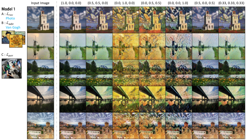
| Model 1 | , Photo | , Van Gogh | , Udnie |
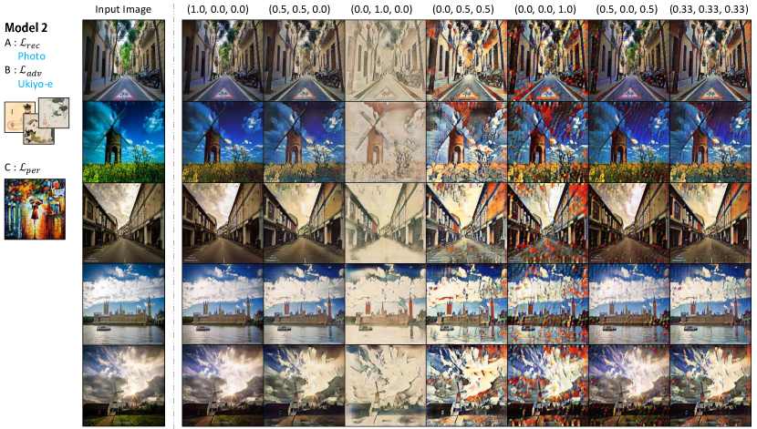
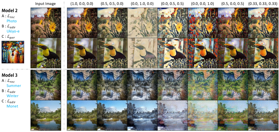
| Model 2 | , Photo | , Ukiyo-e | , Rain |
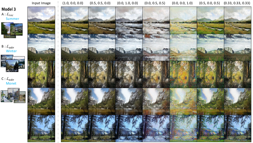
| Model 3 | , Summer | , Winter | , Monet |
Figure 5 shows the results of the experiment. Color-maps on the right sub-figures show computed loss values when weight for each losses are and , respectively. And the plots in each sub-figure denote the results of sym-parameter model (), hyper-parameter models () and an additional ablation (). The figures clearly show the sym-parametrized model properly minimizes weighted losses according to the sym-parameter value. And the results are similar to the multiple hyper-parameter models, which are trained individually. Model uses the sym-parameter as an input, but the weights of each losses are fixed to at training. As the illustrated results show, outputs follow the case regardless of the input because the model did not learn to change the loss function. Also, the same sym-parametrized model is quantitatively compared against various hyper-parameter models that are separately trained. As can be seen in Table 1, the loss values of the models separately trained with hyper-parameterized weights do not differ much from the values of the single model trained with sym-parametrized weights. This implies that a single training of a model using sym-parameters may replace the models trained in multiple cases of hyper-parameters.
5.2 Image Translation to Mixed-Domain
We have set up three SGN models for experiments on image translations to mixed-domain. With the use of sym-parameters, SGN extends the concept of multi-domain to loss functions, and each domain is thus defined with combinations of loss functions and data. For our experiments, the datasets used in [10, 29] are combined with loss criteria of , and from Section 4 to train each model as presented in Table 2.
| Weights | Single sym-parameter model | Hyper-parameter models | ||||||
|---|---|---|---|---|---|---|---|---|
| (1.0, 0.0, 0.0) | 0.164 | 0.164 | 0.829 | 0.209 | 0.159 | 0.159 | 2.540 | 0.252 |
| (0.5, 0.5, 0.0) | 0.305 | 0.285 | 0.323 | 0.253 | 0.407 | 0.423 | 0.391 | 0.270 |
| (0.0, 1.0, 0.0) | 0.211 | 0.756 | 0.211 | 0.311 | 0.308 | 1.008 | 0.308 | 0.276 |
| (0.0, 0.5, 0.5) | 0.171 | 0.718 | 0.256 | 0.085 | 0.205 | 0.924 | 0.247 | 0.163 |
| (0.0, 0.0, 1.0) | 0.040 | 0.443 | 0.525 | 0.040 | 0.015 | 1.039 | 1.375 | 0.015 |
| (0.5, 0.0, 0.5) | 0.139 | 0.201 | 0.889 | 0.077 | 0.117 | 0.184 | 3.054 | 0.050 |
Qualitative Result Figure Sym-parameterized Dynamic Inference for Mixed-Domain Image Translation illustrates translation results of Model 1 with various sym-parameters. Not only inter-translations among A, B and C domains are well generated, but the model also produces mixed generations with weighted characteristics of candidate domains. Especially, the successful image translations between domain B with adversarial loss and domain C with perceptual loss should be noticed; the generated images are influenced more by colors and styles of Van Gogh than by the test image input. As the numbers in the parentheses represent sym-parameter values, correspondingly styled images are well produced when mixed with 3 types of domains. Lastly, generated image with is an extrapolated result with a sym-parameter that is set outside of the trained range, and Van Gogh’s style is still bolstered accordingly.
Figure 6 shows image translations yielded by two other models. While an SGN can be trained with different loss functions and datasets as done for Model 1 and 2, it can also be trained with domains defined with two GAN losses for different datasets. As it can be seen in the figure, Model 3 is able to translate a summer Yosemite image not only to a winter Yosemite image but also to a winter image with Monet style with . This result well depicts how weighted optima of multiple objective functions can be expressed. More test results of each model are provided in the supplementary material.
Quantitative Result It is generally known to be difficult to define quantitatively evaluating metrics for generative models. Nonetheless, it is logical to quantitatively examine by checking loss values for different values since our aim is to find optimal of variously weighted sum of losses. If trained sufficiently in terms of (LABEL:eq:sym-param) and (3), the corresponding domain’s loss should be minimized when a domain’s weight is 1, and when the weight is mid-valued as 0.5, resultant loss of the domain should be valued in between the values when the weight is 1 and 0. Furthermore, we can compare these values with multiple hyper-parameter models that are individually trained.
Loss values of trained Model 1 are measured with a test dataset and enumerated in Table 3. The numbers in the table represent averaged loss values of each loss function the generator uses. In the table, each domain yields its minimum loss value when weighted with 1. And these are similar to the multiple models trained using a corresponding hyper-parameter. The largest difference is that the hyper-parameter models have a high loss value when the weight of a specific loss is zero at the time of testing, such as , while the SGN has a relatively low value. This is because it is advantageous for the SGN to learn that the loss is minimized for similar values such as .
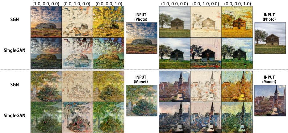
Multiple Datasets vs Multiple Losses We have performed a comparison with SingleGAN [26], which can handle multiple datasets, to clearly show the difference of our multi-loss approach from the conventional methods. For fair comparison, SingleGAN has been trained using Photo as input with three output domains: Photo, Ukiyo-e and Van Gogh. SGN used the reconstruction loss for Photo, GAN losses for Ukiyo-e and Van Gogh. As shown in Figure 7, SingleGan performs style transfer, not reconstruction, for the condition (1,0,0). These results mean that the input images are transferred to Photo style. This can be seen more clearly by using Monet images as input, which are not used for training. In contrast, SGN performs reconstruction for according to the definition of the trained loss, and also operates to reconstruct Monet images that are not used in the training phase at all. This result indicates that SGN behaves according to the loss characteristics learned as we intended.
Continuous Translation Since the sym-parameter is represented as a -dimensional continuous vector, continuous inter-domain translations are achieved during mixed-domain image translations. Such characteristics of SGN allows seamless mixed-domain transitions among candidate domains through the video111https://youtu.be/i1XsGEUpfrs.
5.3 Conditional Channel Attention Module
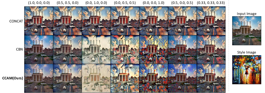
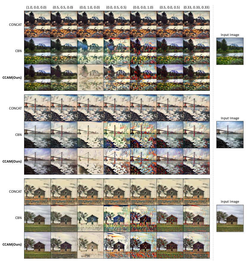
We perform sym-parameter injections into SGN through CCAM since conventional condition injecting methods are empirically shown inefficient for our method. We have thus experimentally compared the performance results among different cases of condition injections, which is depicted in Figure 8. The injection method labeled CONCAT represents the method of depth-wise concatenations with a latent coded vector repeated to be in the same spatial size as features. Central biasing normalization (CBN) [27] is also experimented for comparisons. We have adjusted the instance normalization of the down-sampling layers and the residual blocks of the generator network as similarly used in [26].
CONCAT method produces outputs that are alike despite of various combinations of sym-parameters and fails to generate images in mixed-domain correspondingly. This method works promisingly for discrete condition injections as reported in [3, 15, 30] but struggles in the SGN using continuous conditions. This phenomenon is reasonable considering that the normalization within the generator perturbs the values of the sym-parameter and differences in the values are susceptible. CBN method performs better than CONCAT, generating comparably more various images with given sym-parameters. Yet, its generations are rather biased to one domain than a mixed-domain targeted by sym-parameters, and also follow with some artifacts. Since CBN uses bias and thus is hard to exclude the possibility on influence of a particular channel, additional interferences among candidate domains may occur. Among the experimented condition injecting methods, our proposed CCAM is more suitable for the sym-parameter and SGN.
6 Conclusion
In this paper, we propose a sym-parameter that can extend the concept of domain from data to loss and adjust the weight among multiple domains at inference. We then introduce SGN, which is a novel network that can translate image into mixed-domain as well as each domain using this sym-parameter. It is hard to say which method is proper and optimal when it comes to making a valid result for a mixed-domain without ground truth. However, if optimizing to the weighted objective of each domain is one of the effective methods for this purpose, SGN performs well to translate image to a target mixed-domain as shown in the experiments. We expect that the research will be extended to apply sym-parameter to more diverse domains, and to find more effective models for sym-parameter.
Acknowledgement
This work was supported by Next-Generation Information Computing Development Program through the National Research Foundation of Korea (NRF-2017M3C4A7077582).
References
- [1] David Berthelot, Thomas Schumm, and Luke Metz. Began: boundary equilibrium generative adversarial networks. arXiv preprint arXiv:1703.10717, 2017.
- [2] Xi Chen, Yan Duan, Rein Houthooft, John Schulman, Ilya Sutskever, and Pieter Abbeel. Infogan: Interpretable representation learning by information maximizing generative adversarial nets. In Advances in neural information processing systems, pages 2172–2180, 2016.
- [3] Yunjey Choi, Minje Choi, Munyoung Kim, Jung-Woo Ha, Sunghun Kim, and Jaegul Choo. Stargan: Unified generative adversarial networks for multi-domain image-to-image translation. arXiv preprint, 1711, 2017.
- [4] Alexey Dosovitskiy, Jost Tobias Springenberg, Maxim Tatarchenko, and Thomas Brox. Learning to generate chairs, tables and cars with convolutional networks. IEEE transactions on pattern analysis and machine intelligence, 39(4):692–705, 2017.
- [5] Ahmed Elgammal, Bingchen Liu, Mohamed Elhoseiny, and Marian Mazzone. Can: Creative adversarial networks, generating” art” by learning about styles and deviating from style norms. arXiv preprint arXiv:1706.07068, 2017.
- [6] Ian Goodfellow, Jean Pouget-Abadie, Mehdi Mirza, Bing Xu, David Warde-Farley, Sherjil Ozair, Aaron Courville, and Yoshua Bengio. Generative adversarial nets. In Advances in neural information processing systems, pages 2672–2680, 2014.
- [7] Kaiming He, Xiangyu Zhang, Shaoqing Ren, and Jian Sun. Deep residual learning for image recognition. In Proceedings of the IEEE conference on computer vision and pattern recognition, pages 770–778, 2016.
- [8] Jie Hu, Li Shen, and Gang Sun. Squeeze-and-excitation networks.
- [9] Phillip Isola, Jun-Yan Zhu, Tinghui Zhou, and Alexei A Efros. Image-to-image translation with conditional adversarial networks. arXiv preprint, 2017.
- [10] Justin Johnson, Alexandre Alahi, and Li Fei-Fei. Perceptual losses for real-time style transfer and super-resolution. In European Conference on Computer Vision, pages 694–711. Springer, 2016.
- [11] Tero Karras, Timo Aila, Samuli Laine, and Jaakko Lehtinen. Progressive growing of gans for improved quality, stability, and variation. arXiv preprint arXiv:1710.10196, 2017.
- [12] Taeksoo Kim, Moonsu Cha, Hyunsoo Kim, Jung Kwon Lee, and Jiwon Kim. Learning to discover cross-domain relations with generative adversarial networks. arXiv preprint arXiv:1703.05192, 2017.
- [13] Diederik P Kingma and Max Welling. Auto-encoding variational bayes. arXiv preprint arXiv:1312.6114, 2013.
- [14] Mark A Kramer. Nonlinear principal component analysis using autoassociative neural networks. AIChE journal, 37(2):233–243, 1991.
- [15] Guillaume Lample, Neil Zeghidour, Nicolas Usunier, Antoine Bordes, Ludovic Denoyer, et al. Fader networks: Manipulating images by sliding attributes. In Advances in Neural Information Processing Systems, pages 5967–5976, 2017.
- [16] Christian Ledig, Lucas Theis, Ferenc Huszár, Jose Caballero, Andrew Cunningham, Alejandro Acosta, Andrew P Aitken, Alykhan Tejani, Johannes Totz, Zehan Wang, et al. Photo-realistic single image super-resolution using a generative adversarial network. In CVPR, volume 2, page 4, 2017.
- [17] Xudong Mao, Qing Li, Haoran Xie, Raymond YK Lau, Zhen Wang, and Stephen Paul Smolley. Least squares generative adversarial networks. In Computer Vision (ICCV), 2017 IEEE International Conference on, pages 2813–2821. IEEE, 2017.
- [18] Mehdi Mirza and Simon Osindero. Conditional generative adversarial nets. arXiv preprint arXiv:1411.1784, 2014.
- [19] Augustus Odena, Christopher Olah, and Jonathon Shlens. Conditional image synthesis with auxiliary classifier gans. arXiv preprint arXiv:1610.09585, 2016.
- [20] Guim Perarnau, Joost van de Weijer, Bogdan Raducanu, and Jose M Álvarez. Invertible conditional gans for image editing. arXiv preprint arXiv:1611.06355, 2016.
- [21] Alec Radford, Luke Metz, and Soumith Chintala. Unsupervised representation learning with deep convolutional generative adversarial networks. arXiv preprint arXiv:1511.06434, 2015.
- [22] Olaf Ronneberger, Philipp Fischer, and Thomas Brox. U-net: Convolutional networks for biomedical image segmentation. In International Conference on Medical image computing and computer-assisted intervention, pages 234–241. Springer, 2015.
- [23] Karen Simonyan and Andrew Zisserman. Very deep convolutional networks for large-scale image recognition. CoRR, abs/1409.1556, 2014.
- [24] Kihyuk Sohn, Honglak Lee, and Xinchen Yan. Learning structured output representation using deep conditional generative models. In Advances in Neural Information Processing Systems, pages 3483–3491, 2015.
- [25] Yaniv Taigman, Adam Polyak, and Lior Wolf. Unsupervised cross-domain image generation. arXiv preprint arXiv:1611.02200, 2016.
- [26] Xiaoming Yu, Xing Cai, Zhenqiang Ying, Thomas Li, and Ge Li. Singlegan: Image-to-image translation by a single-generator network using multiple generative adversarial learning. arXiv preprint arXiv:1810.04991, 2018.
- [27] Xiaoming Yu, Zhenqiang Ying, Ge Li, and Wen Gao. Multi-mapping image-to-image translation with central biasing normalization. arXiv preprint arXiv:1806.10050, 2018.
- [28] Han Zhang, Tao Xu, Hongsheng Li, Shaoting Zhang, Xiaolei Huang, Xiaogang Wang, and Dimitris Metaxas. Stackgan: Text to photo-realistic image synthesis with stacked generative adversarial networks. arXiv preprint, 2017.
- [29] Jun-Yan Zhu, Taesung Park, Phillip Isola, and Alexei A Efros. Unpaired image-to-image translation using cycle-consistent adversarial networks. arXiv preprint, 2017.
- [30] Jun-Yan Zhu, Richard Zhang, Deepak Pathak, Trevor Darrell, Alexei A Efros, Oliver Wang, and Eli Shechtman. Toward multimodal image-to-image translation. In Advances in Neural Information Processing Systems, pages 465–476, 2017.
Supplementary Material
A Experiment Settings
A.1 1D Toy Example
The polynomial and the linear function are defined such that the output is between 0 and 1 when the range of is -1 to 1.
| (6) |
| (7) |
The sym-parametrized network is an MLP network that has three hidden layers with the size of 64 and ReLU activations. It takes a tuple of as an input and outputs a single value for either classification or regression. The mean squared error function is used for regression loss , and binary cross entropy is used for the classification loss . is scaled down to 20% to balance the losses. In the training phase, the sym-parameter is sampled from Dirichlet distribution with valued (0.5, 0.5). We use ADAM with a batch size of 16, and learning rates of 0.01 during the first 200 epochs, 0.001 during the next 200 epochs and 0.0001 during the last 100 epochs.
A.2 Sym-Parameterized Generative Network
For three loss terms, , and , we use norm for the reconstruction loss , and have applied a technique of LSGAN [17] for the adversarial loss in which an MSE (mean squared error) loss is used. Additionally, the identity loss introduced by Taigman et al. [25] and used in CycleGAN [29] is used in for regularizing the generator, combined with the LSGAN loss. The implementation of the perceptual loss follow the implementation of Johnson et al. [10], adopting both feature reconstruction loss and style reconstruction loss. At the training phase, all three loss terms were weighted by numbers sampled from Dirichlet distribution with all the valued 0.5.
The architecture details of an SGN generator is provided in Table 4 of this supplementary. The discriminator is equivalently set as CycleGAN [29]. To regulate the imbalance between the losses, and are respectively weighted with 2 and 1. And for , GAN loss and the identity loss are respectively weighted by 1 and 5. For the perceptual loss , we have used the pretrained Pytorch model of VGG16 [23] without batch-normalization layers. is composed of a content loss and a style loss, computed at first 4 blocks of VGG16, which means it uses output features from Conv1-2, Conv2-2, Conv3-3, Conv4-3, and do not use the fifth block, following the work of Johnson et al. [10]. The content loss is weighted with 0.001 and the style losses at 4 layers are weighted as (0.1, 1.0, 10, 5.0) for the Model 1, (0.1, 1.0, 10, 5.0) for the other models. We use the ADAM optimizer with a batch size of 4. Then Model 1 and Model 2 are trained for 20 epochs and Model 3 is trained for 60 epochs. We keep the learning rate of 0.0002 for the first half of epochs and linearly decay it to zero for the remaining epochs. Source code and pre-trained networks are available in https://github.com/TimeLighter/pytorch-sym-parameter.
| Layer Configuration | Input Dimension | Layer Information | Output Dimension |
| Input convolution | (, , 3) | Convolution (K:7x7, S:1, P:3), IN, ReLU | (, , 64) |
| CCAM (Reduction Rate : 4) | |||
| Down-sampling | (, , 64) | Convolution (K:3x3, S:2, P:1), IN, ReLU | (, , 128) |
| (, , 128) | Convolution (K:3x3, S:2, P:1), IN, ReLU | (, , 256) | |
| CCAM (Reduction rate : 4) | |||
| Residual Blocks | (, , 256) | Convolution (K:3x3, S:1, P:1), IN, ReLU | (, , 256) |
| (, , 256) | Convolution (K:3x3, S:1, P:1), IN, ReLU | (, , 256) | |
| (, , 256) | Convolution (K:3x3, S:1, P:1), IN, ReLU | (, , 256) | |
| (, , 256) | Convolution (K:3x3, S:1, P:1), IN, ReLU | (, , 256) | |
| (, , 256) | Convolution (K:3x3, S:1, P:1), IN, ReLU | (, , 256) | |
| (, , 256) | Convolution (K:3x3, S:1, P:1), IN, ReLU | (, , 256) | |
| (, , 256) | Convolution (K:3x3, S:1, P:1), IN, ReLU | (, , 256) | |
| (, , 256) | Convolution (K:3x3, S:1, P:1), IN, ReLU | (, , 256) | |
| (, , 256) | Convolution (K:3x3, S:1, P:1), IN, ReLU | (, , 256) | |
| CCAM (Reduction Rate : 4) | |||
| Up-sampling | (, , 256) | Transposed Convolution (K:3x3, S:2, P:1), IN, ReLU | (, , 128) |
| (, , 128) | Transposed Convolution (K:3x3, S:2, P:1), IN, ReLU | (, , 64) | |
| Output Convolution | (, , 64) | Convolution (K:7x7, S:7, P:3), Tanh | (, , 3) |
B Additional Experimental Results
B.1 Tradeoff with Network Size
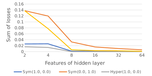
Using sym-parameter does not always have tradeoffs in performance, but it is affected by the capacity of the model. Figure 9 shows the losses when changing the number of filters in the 1D Toy problem. As the size of the model decreases, the loss is getting larger than the hyper-parameter models. However, considering that a single sym-parameter model can be used as multiple hyper-parameter models with a specific range of weights, the difference is not significant.
B.2 Continuous Translation
The video (https://youtu.be/i1XsGEUpfrs) is created by extracting images from the original and translating it through SGN. ORIGINAL VIDEO and VIDEO WITH SGN represent original video and SGN translated video, respectively. We use SGN models trained in the paper and translated images changing only the sym-parameters. The color bar above VIDEO WITH SGN represents the sym-parameter values for each domain. If the entire bar is red, then the sym-parameter is (1,0,0). Since all the images are translated through SGN, reconstructed images may differ in some colors and appearance from the original ones.
B.3 More Results of CCAM
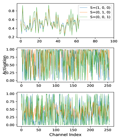
Figure 10 summarizes channel activation trends of CCAM when changing sym-parameters for a given test image. As can be seen in the plots, channels are activated differently for three cases of sym-parameter. First layer of CCAM is mainly responsible for scaling with no blocked channel. Considering the number of closed channels with zero activations are increased at deeper layers, CCAM selectively excludes channels and reduces influence of unnecessary channels to generate images in a mixed-domain conditioned by sym-parameters. This is the major difference of our CCAM and the CBN which utilizes bias in controlling each domain’s influence. Figure 11 is additional images according to the sym-parameter injection method.

B.4 More Results of Image Translation
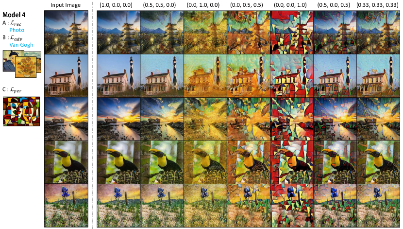
Figure 12, 13 and 14 shows additional images for models 1, 2, and 3 of the paper, respectively. Figure 15 is the results of the new SGN model not in the paper.
