Unimolecular FRET Sensors: Simple Linker Designs and Properties

Abstract

Protein activation and deactivation is central to a variety of biological mechanisms, including cellular signaling and transport. Unimolecular fluorescent resonance energy transfer (FRET) probes are a class of fusion protein sensors that allow biologists to visualize using an optical microscope whether specific proteins are activated due to the presence nearby of small drug-like signaling molecules, ligands or analytes. Often such probes comprise a donor fluorescent protein attached to a ligand binding domain, a sensor or reporter domain attached to the acceptor fluorescent protein, with these ligand binding and sensor domains connected by a protein linker. Various choices of linker type are possible ranging from highly flexible proteins to hinge-like proteins. It is also possible to select donor and acceptor pairs according to their corresponding Föster radius, or even to mutate binding and sensor domains so as to change their binding energy in the activated or inactivated states. The focus of the present work is the exploration through simulation of the impact of such choices on sensor performance.

1 Introduction

Measurement of biomarkers and ligands are increasingly used to study transport, signaling and communication in cells, and as diagnostics/prognostics of disease, or the presence of pathogens, allergens and pollutants in foods, and the environment. Accurate measurement in assays or cellular environments is important, and protein based biosensors can be used in this context. But due to the molecular complexity of such sensors,understanding the features that determine their performance is difficult both from the perspective of experiment, and detailed molecular dynamics. In the latter case this is due to the size of the system to be simulated and the associated time and spatial scales. To investigate such systems, at a qualitative level we use simple coarse grained models of proteins, and for critically important features requiring high accuracy, we employ advanced molecular dynamics, in particular rare-event methods.

Fluorescence (or Föster) resonance energy transfer (FRET) occurring between donor and acceptor fluorescent protein (FP) pairs can provide detailed spatio-temporal information about a wide range of biological processes. Typically, the FRET efficiency, $\cal I$ the average fraction of energy transfer events per donor excitation event - falls off quickly with distance between the FPs near the so called Föster radius, $R_{0}\sim 5-7$ nm, thus offering a highly sensitive indicator of spatial and temporal change between the FP pair. Biosensors incorporating FP pairs can be designed to respond to variations in local concentrations of target analytes (small signaling molecules or biomarkers), that change the internal structure of the biosensor, bringing the FPs closer on average, which in turn can be observed optically through changes in the FRET efficiency.

Many unimolecular FRET based probes designed to monitor or report the local concentrations of analytes, comprise a donor FP attached to a ligand binding domain, a sensor or reporter domain attached to the acceptor FP, with these ligand binding and sensor domains connected by a linker (see Fig.1 for three examples). When the ligand binding domain is activated due to the proximity of a ligand or analyte (the so called ON state), an attractive interaction is turned on between the binding and sensor domains causing them to come together, bringing their donor and acceptor FPs closer. In the absence of the ligand/analyte (the OFF state), the domains should remain further apart. Such spatial changes can be measured by changes in the FRET efficiency between the FPs.

How well one can discriminate between the background or basal efficiency ${\cal I}_{0}$, and changes in the FRET efficiency due to changes in the analyte concentration close to the sensor is determined by the signal-to-noise ratio $({\cal I}-{\cal I}_{0})/{\cal I}_{0}=\Delta{\cal I}/{\cal I}_{0}$, and is of critical importance in sensor design. A related quantity is ${\cal J}=\frac{\sigma({\cal I}-\cal{I}_{0})}{\mu({\cal I}-{\cal I}_{0})}$ (i.e. the fractional error in the gain $\mu({\cal I}-{\cal I}_{0})$) which is simply related to the so called Z’ factor used to characterise the quality of a sensor. In particular, one can easily show (making reasonable assumptions) that the fractional error in the ligand/biomarker concentration predicted from calibrated FRET measurements is proportional to $\cal J$. Here $\mu$ and $\sigma$ denote the mean and the variance. This allows the effect of changes in the sensor design to be easily related to the accuracy at which concentrations of target ligands/biomarkers can be measured.

The choice of molecular linker used to connect the components B and B’ of the biosensor depicted in the top panels of Fig. 1 can have a strong influence on its overall performanceLissandron et al. (2005). In this current work we first model the flexible linker system developed by Komatsu et al. (2011) using a variable numbers of repeat units of the form (SAGG)_n to design a FRET biosensor for Kinases and GTPases. We then compare these results with idealized models of hinge type linkers built using $\alpha$-helical proteins. This will allow four general design questions to be considered. First, can a simple mechanistic model of the Komatsu sensor capture the salient features observed in experiment? Second, for unimolecular sensors, is there an advantage in replacing the flexible linker peptide of Komatsu et al. (2011) with a hinge peptide? Third, to enhance precision of measurement, is it in principle better to increase of decrease the the Föster radius of fluorescent proteins? Fourth, is precision enhanced or reduced if the binding energy of the ligand and sensor domains is attractive or repulsive in the absence of the target ligand?

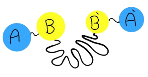
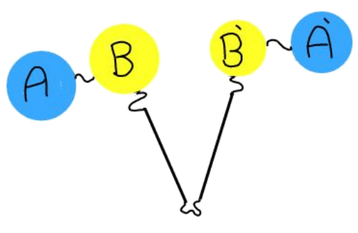
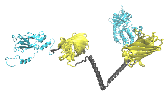
Figure 1: Top-left is a schematic illustration of a unimolecular sensor where a flexible linker is used to connect protein modules B and B’. Top-right corresponds to the case where the flexible linker is replaced by a free hinge type protein. The bottom figure is an example of a PKA sensor where the yellow cylindrical-like proteins flanking the hinge are FP’s; and the sensing units are the PKA substrate (far left) and corresponding consensus protein respectively (far right). When the PKA substrate is phosphorylated by PKA, it will bind to the consensus protein. Note frequently the order of A,A’ and B,B’ is interchanged.

2 Methods

To analyse experimental FRET microscopy results, and more generally, to explore idealized design motifs for chromophore - linker - chromophore systems, we have built simplified models of unimolecular FRET probes, represented by two macro-particles joined by an idealized linker. One spherical macro-particle represents the donor fluorophore attached to the ligand binding domain and the other represents the acceptor fluorophore attached to the signaling domain. The macro-particles are connected to either end of a peptide linker, which may be flexible, or “hinge-like” modeling strong secondary structures such as a pair of flexibly connected or hinged alpha helices Boersma et al. (2015).

The spherical macro-particles interact through a pair potential of the form

$$V(R)=V_{s}(R)+V_{\ell}(R)$$ (1)

where the first term denotes binding between the macro-particles due to the presence of the target ligand/analyte, and the second term is an interaction specific to each linker type. When the ligand binding domain is in the OFF or basal state, $V_{s}$ ensures that the spherical macro-particles cannot overlap, $V_{s}(R)=\infty$ if $R<\sigma$ and is zero otherwise. When the signal domain is in ON state, $V_{s}$ has, in addition to this excluded volume interaction, an attractive square well interaction of depth $\epsilon$ for $\sigma<R<\sigma+\Delta$, where $R=|\vec{R}_{2}-\vec{R}_{1}|$ is the distance between the macro-particles. The protein diameter defined as $\sigma$, is used as the unit of length. The Föster Radius $R_{0}$ is assumed to be 2.5 times greater than $\sigma$, and $\Delta$, the width of the attractive well, is set at 0.2$\sigma$. The binding energy in the ON state is specified by $\epsilon$, which is given in terms of $k_{B}T$, where $T$ corresponds to physiological temperature of 309K.

Flexible linker

With the flexible linker model the two spherical macro-particles with excluded diameter $\sigma$ represent the FRET fluorophores and their associated proteins. The form of $V_{s}$ has been defined above, and the linker part of the interaction is a simple isotropic pair potential with the form

$$V_{\ell}(|\vec{R}_{2}-\vec{R}_{1}|)=\begin{cases}\infty&\mbox{ if }R>{\cal L}\\ 0&\mbox{otherwise }\end{cases}$$ (2)

Geometrically this can be visualized as two non-overlapping macro-particles free to move inside a sphere of diameter $\cal L$. To compare FRET efficiency predictions of the simple flexible linker model with experiment where the linker length is given as the total number of residues $\cal N$, it is necessary to relate $\cal N$ to $\cal L$. This was done through their corresponding mean square center-to-center distances, $\langle R^{2}\rangle$ (see appendix B ). Sanyal et al. (2016)

For the experimental system, if the linker is sufficiently flexible, the center-to-center distance can be approximated as a Gaussian random walk for which

$$\langle R^{2}\rangle=D_{0}^{2}+C_{\infty}{\cal N}b_{0}^{2},$$ (3)

where $D_{0}$ is the diameter of the macro-particles, $C_{\infty}$ is the characteristic ratio, and $b_{0}$ is the distance between consecutive C-$\alpha$ atoms in the peptide chainSanyal et al. (2016); Evers et al. (2006). The corresponding Kuhn length of the model is given by $C_{\infty}b_{0}$, and is applicable to flexible peptides. As we have seen in Fig. 2, we find that once $\cal L$ is related to $\cal N$ in this way, there is very close correspondence between the prediction of the model and the experiment results with only slight differences occurring when the linker is short arising as a consequence of departure from the ideal Gaussian chain behavior, see Fig. S1(b) in A for further details. Sanyal et al. (2016)

Spherical hinge linker

For the spherical hinge linker, $V_{\ell}(|\vec{R}_{2}-\vec{R}_{1}|)$ simply corresponds to two rods of equal length $\frac{\cal L}{2}$ connected by a freely rotating joint at the origin, or equivalently to the constraints ${x_{1}}^{2}+{y_{1}}^{2}+{z_{1}}^{2}=\frac{L^{2}}{4}={x_{2}}^{2}+{y_{2}}^{2}+{z_{2}}^{2},$ which geometrically can be viewed as two non-overlapping macro-particles free to move on the surface of a sphere of diameter $\cal L$.

Circular hinge linker

For the circular hinge linker model, $V_{\ell}(|\vec{R}_{2}-\vec{R}_{1}|)$ is similar to that of the spherical hinge, with the additional constraints that $z_{1}=0=z_{2}$, which geometrically corresponds to two non-overlapping macro-particles free to move on a circle of diameter $\cal L$.

Observables and sampling procedure

The distance dependence of the FRET efficiency is approximated by the expression,

$$I(R)={1\over 1+(R/R_{0})^{6}}$$ (4)

with the Föster radius $R_{0}\sim 5-7$ nm giving the distance at which the energy transfer efficiency is $50\%$ and $R$ is the distance between the spherical macro-particles. To calculate the efficiency, as measured in the experiment, we compute its expectation value so ${\cal I}=\langle I(R)\rangle$ where the angle brackets indicate the corresponding average over the Boltzmann distribution either the the OFF and ON states. The Föster radius $R_{0}$ depends on various quantities including: the fluorescence quantum yield of the donor in the absence of the acceptor, the refractive index of the medium, and the dipole orientation factor $\langle\kappa^{2}\rangle$ (see section B). We use the Monte Carlo simulation approach Metropolis et al. (1953); Frenkel and Smit. (1996); Corry et al. (2005) to estimate the statistical properties of each model. Further details of the observable, underlying theoretical assumptions and the sampling procedure are given in B.

3 Results

The influence of different geometrical/structural properties of linkers on the FRET efficiency is explored here using simple statistical mechanics models and Monte Carlo simulations.

Comparison of Simulation & Experiment for the flexible linker

In Fig.2 we compare the results of our flexible linker model simulations with the experimental findings for both signal (a), and signal-to-noise ratio (b) obtained by Komatsu et al. (2011) as a function of linker length. The comparison give consistent estimates for the ON state binding energy for this particular experimental system of $\epsilon=2.5$ $k_{B}T$. In panel (c) $\cal J$ is plotted as a function of effective number of residues $N_{Eff}$.

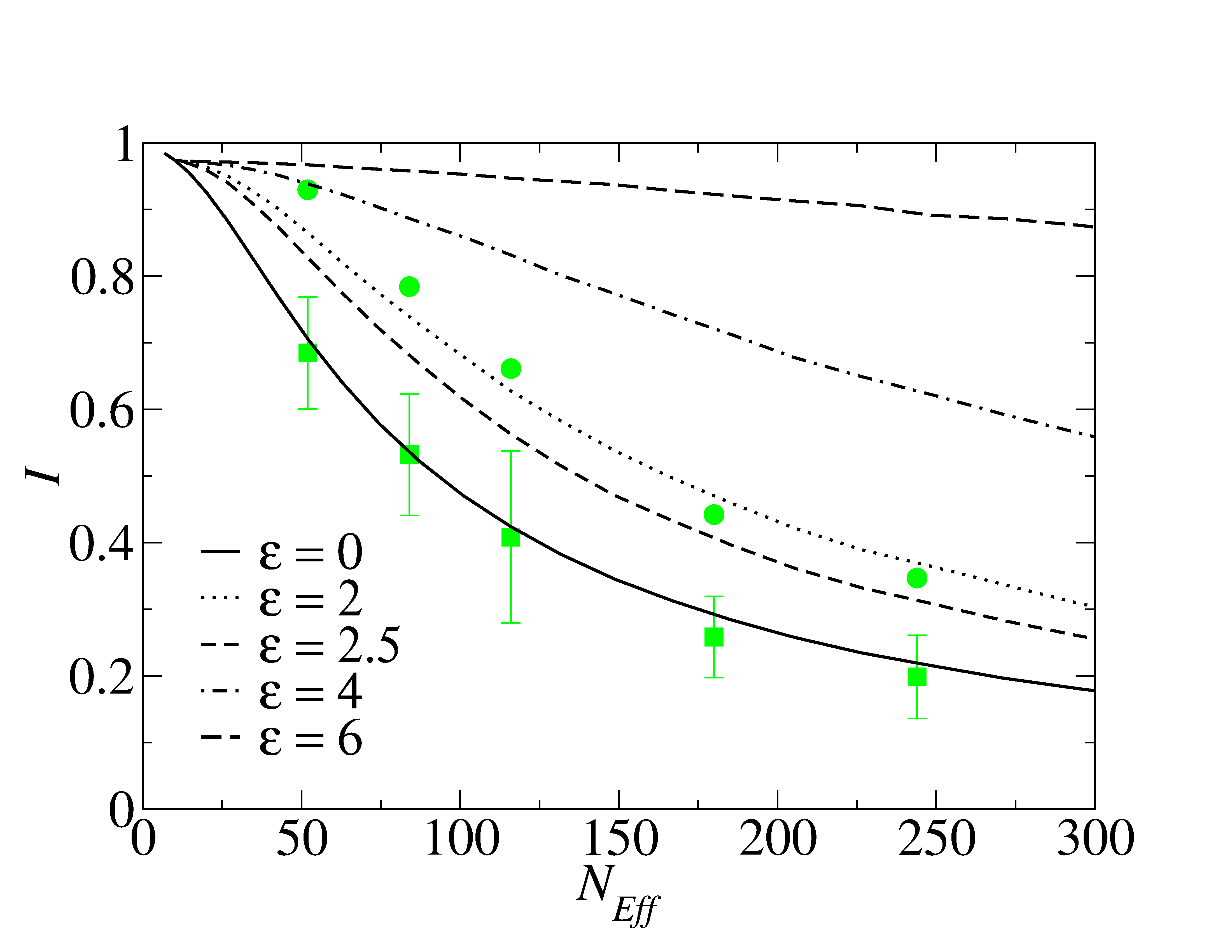
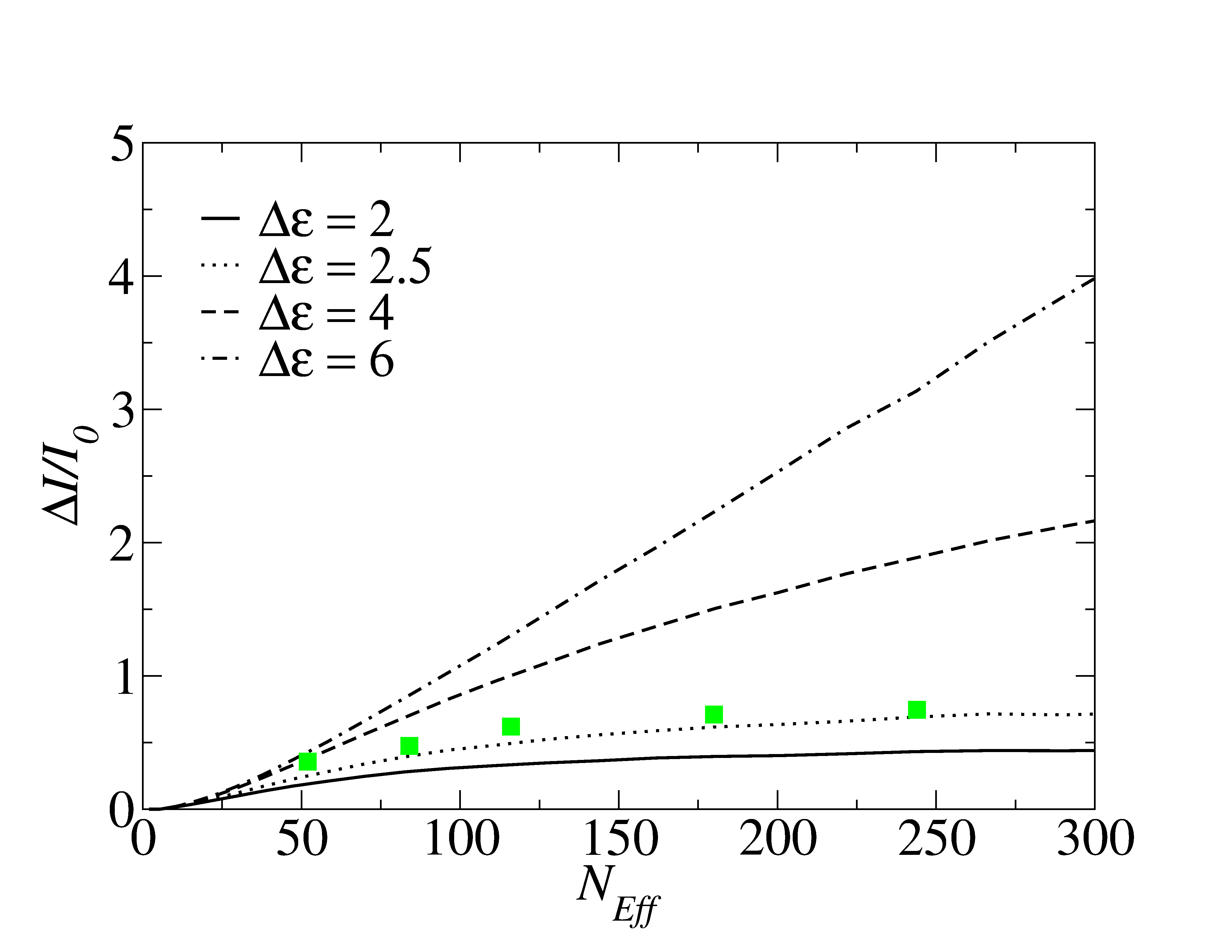
(a) (b)
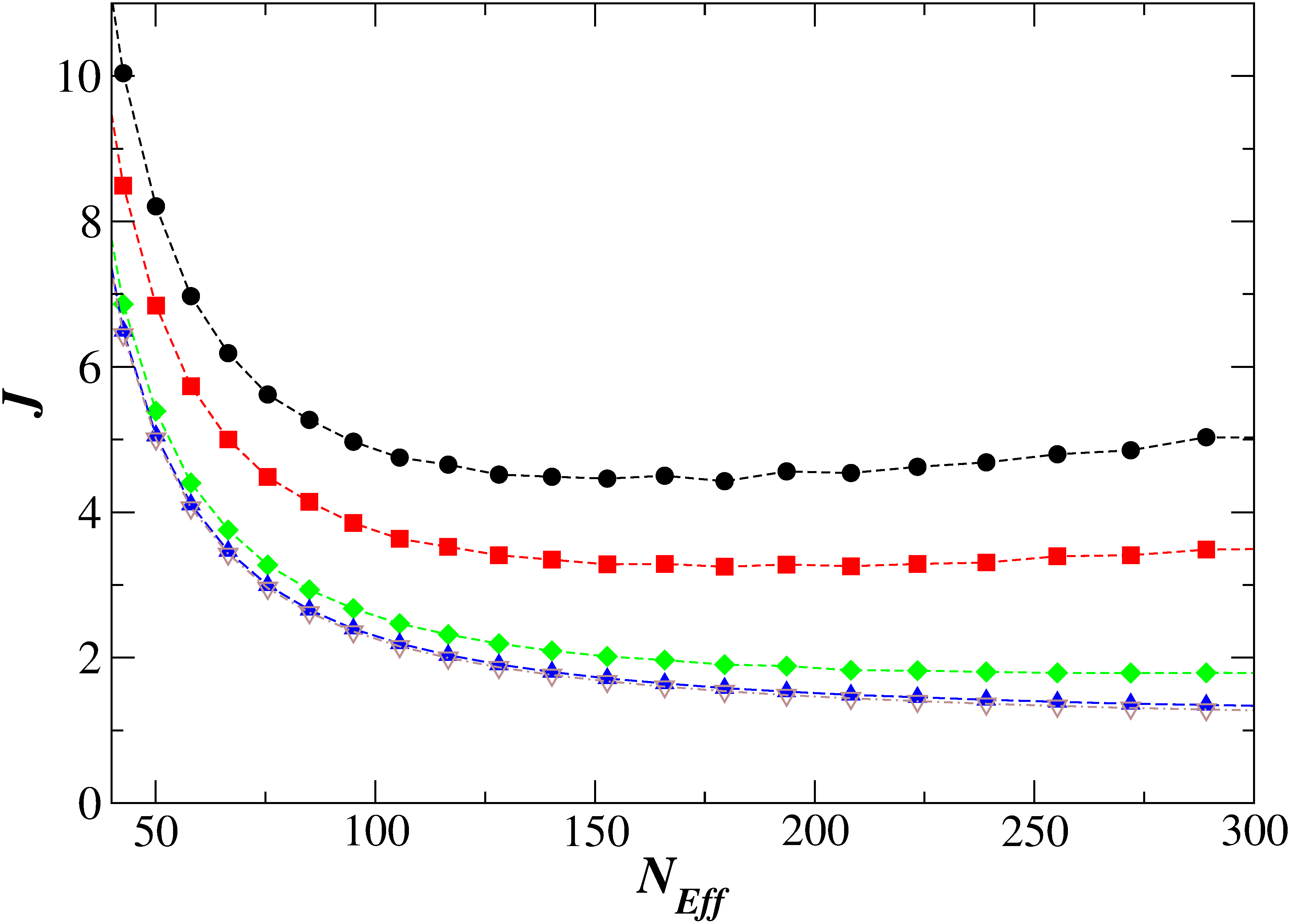
(c)

Figure 2: (a) FRET intensity $\cal I$ of the flexible linker model as a function of number of linker residues. Results are presented for five different values of the binding energy $\epsilon$, where $\epsilon=0$ corresponds to the basal case. Data from experiments Komatsu et al. (2011), in the OFF or basal state (filled green squares) and in the ON state (filled green circles) are superimposed on the theoretical predictions. (b) Corresponding signal-to-noise $\Delta{\cal I}/{\cal I}_{0}$ for the theoretical model overlaid with the experimental signal-to-noise ratio data (filled green squares). (c) ${\cal J}$ of the flexible linker model as a function of effective number of residues $N_{Eff}$. The lower the value of $\cal J$, the more accurate the sensor, where each curve corresponds to a value of $\epsilon$, black bullet 2; red square 2.5; blue lozenge 4; and green triangle 6 (in units of $k_{B}T$).

Comparison of sensor performance for flexible and hinge linkers

To compare the performance of sensors when the flexible linker between B and B’ is replaced by a free hinge, we demanded that the arms of each hinge consist of about 28 residues (alpha helices of this length can be selected that are structurally stable) and that the flexible linker correspond to the optimal linker of Komatsu et al. (2011) , which was 116 residues in length. Fig 3 (a) shows that under such assumptions, the signal to noise ratio’s where free hinge linkers are used instead of flexible linkers are significantly higher. Fig 3 (b) which plots $\cal J$ indicates that hinge linker based sensors for moderate and high binding energies are likely go give rise to much more precise sensors. Examples of such hinge proteins include those reported by Boersma et al. (2015),and behave as free spherical hinges (the detailed free energy simulation results are not displayed here due to space limitations).

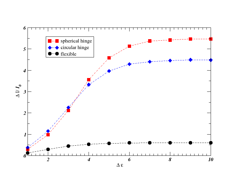
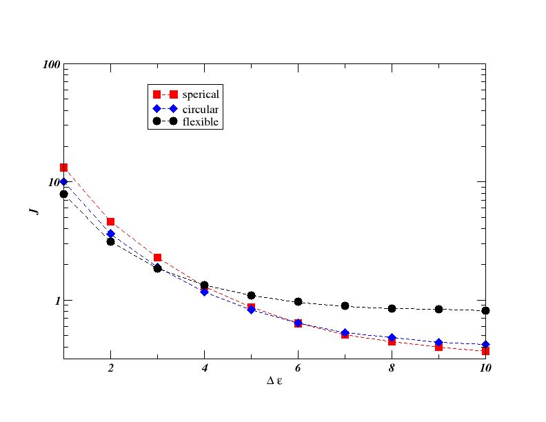
(a) (b)

Figure 3: $\Delta{\cal I}/{\cal I}_{0}$ (left panel) and $\cal J$ (right panel) are plotted for the spherical hinge, circular hinge and flexible linker sensors respectively for ${\cal L}=3.48\,\sigma$. For flexible linkers of Komatsu et al. (2011) this correspond to 116 amino-acids/residues, and for hinge linker sensors, this correspond to length for each arm of 4.2 nm or equivalently 28 amino-acids, each arm being an alpha helix.

Role of Föster radius on sensor performance

While the FRET efficiency for all systems must increase with increasing $R_{0}$, as is observed in experiments, Visser et al. (2003) it is not clear how the signal-to-noise ratio should vary. Calculation results for our model system (see Fig. 4) show that $\Delta{\cal I}/{\cal I}_{0}$ decreases and $\cal J$ increases dramatically with increasing $R_{0}$. This suggests that trying to increase signal to noise by increasing the $R_{0}$ can be counter-productive. Instead, reducing the Föster radius where possible is likely to significantly enhance sensor accuracy.

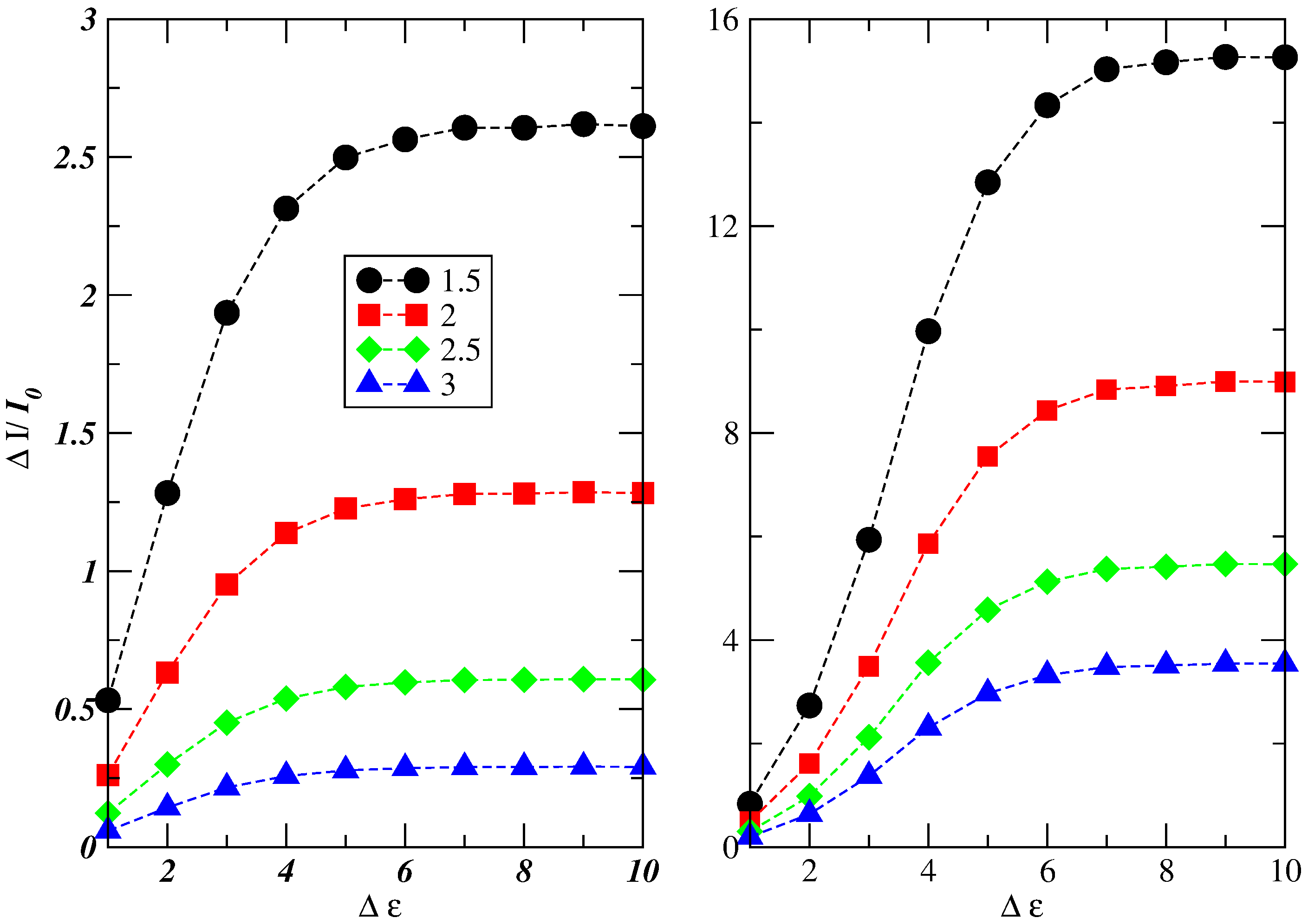
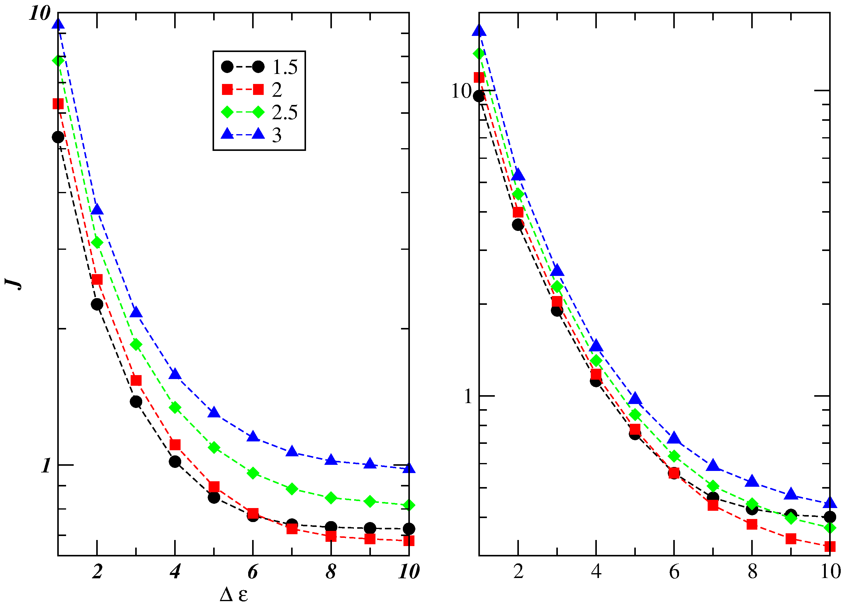
Figure 4: Signal-to-noise $\Delta{\cal I}/{\cal I}_{0}$ (top panels) and fractional error in the gain $\cal J$ (bottom panels) as a function of Föster Radius $R_{0}$, with ${\cal L}=3.48\,\sigma$ (corresponding to the flexible linker sensor consisting of 116 residues of Komatsu et al. (2011) (left panels) and spherical hinge sensors (right panels) where each arm of the hinge is of length 4.2 nm).

Effect of non-zero basal binding energy

For simplicity, we have assumed that in the OFF or basal state the only interaction between the ligand binding and sensor domains is a hardcore repulsion preventing their overlap, and correspondingly set the binding energy $\epsilon$ between spherical macro-particles to zero in the OFF state. However, an additional attractive or repulsive interaction is possible even in the absence of the ligand/analyte. This can be modeled as non-zero basal binding energy $\epsilon_{0}$ by using an attractive or repulsive square well potential. The dependence of the signal-to-noise ratio $\Delta{\cal I}/{\cal I}_{0}$ and the square root of the variance of $\Delta{\cal I}\equiv{\cal J}$ respectively on the difference in binding energy between the ON and OFF states $\Delta\epsilon$ is displayed in Fig.5. For low values of $\cal L$, the effects on $\Delta{\cal I}/{\cal I}_{0}$ are not appreciable, however for larger values it is evident that varying -$\epsilon_{0}$ from -1 to 1 is reduced by more than half. $\cal J$ is high where $\Delta{\cal I}/{\cal I}_{0}$ is low and vica-versa, which is what one would expect intuitively. $\cal J$ is sensitive to variations in low values of $\Delta\epsilon$, in particular when the basal interaction is repulsive. For moderate to high values of $\Delta\epsilon$ $\cal J$ is significantly lower when the basal interaction is repulsive, but only marginally in comparison with the neutral case of no interaction.

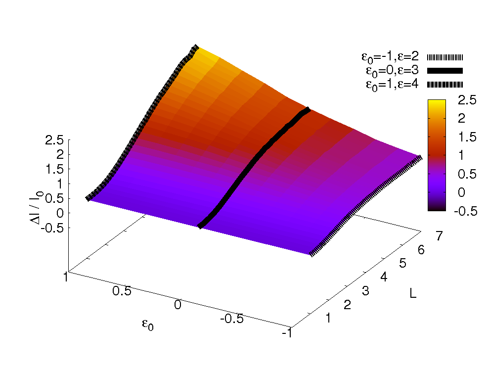
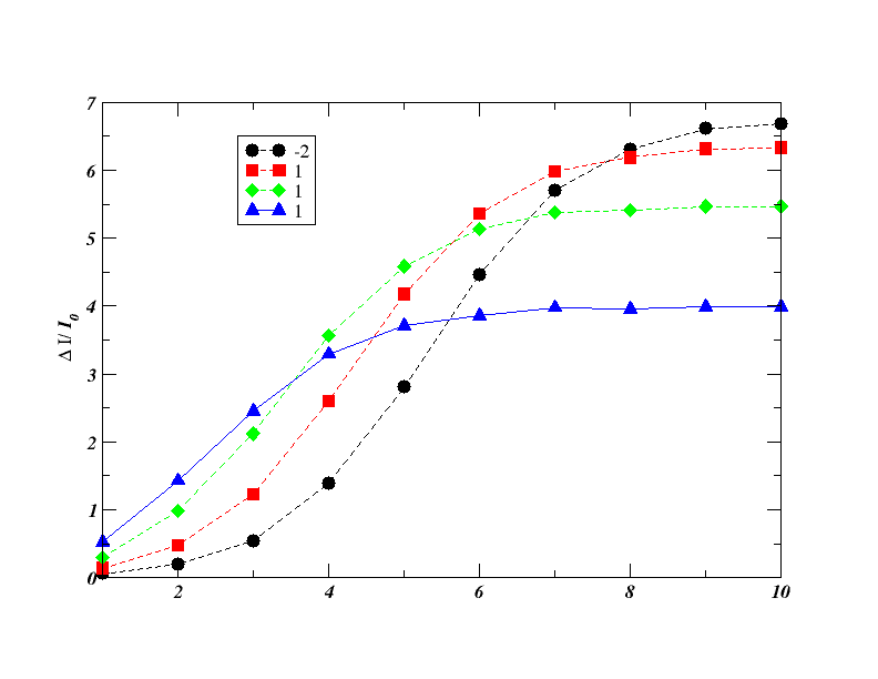
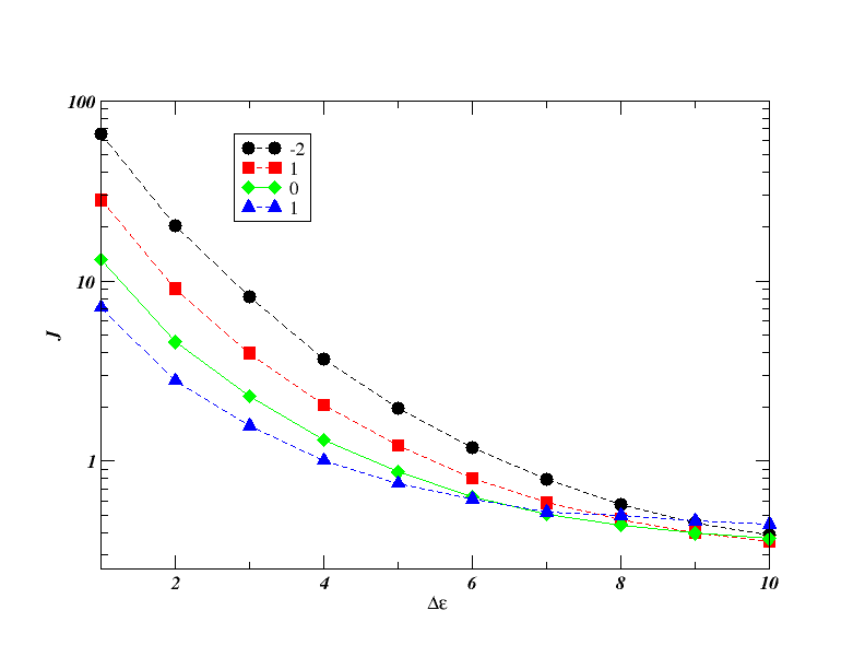
(a)
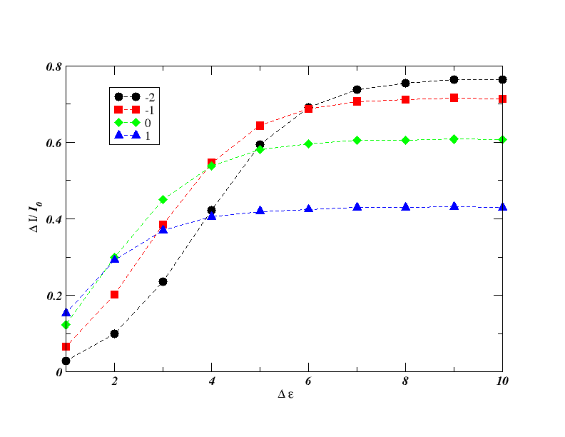
(b) (c)
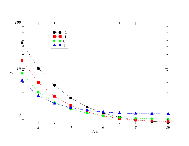
(d) (e)

Figure 5: (a) $\Delta{\cal I}/{\cal I}_{0}$ and $\cal J$ of the flexible linker, spherical hinge linker and circular hinge linker model sensors as a function of basal binding energy $\epsilon_{0}$ varying from -2k_bT to 1k_bT, and in the top panel(a) for the flexible linker sensor model also as a function $\cal L$ in units of macro particle diameter $\sigma$. Dependence of the $\Delta{\cal I}/{\cal I}_{0}$ (figures a, b and c) and $\cal J$ (figures d and e) respectively on $\Delta\epsilon$ for ${\cal L}=3.48\,\sigma$ and representative values of $\epsilon_{0}$ for the flexible linker, spherical hinge linker sensors respectively.

4 Conclusion and Outlook

In this work general design features of unimolecular FRET sensors were explored using simple coarse grained models and Monte Carlo Simulation. The starting point was the successful modeling of such sensors where highly optimized flexible linkers of Komatsu et al. (2011) are used to connect the ligand binding and sensor domains. The flexible linker proteins were then replaced by hinge like proteins where each arm is rod like, for example has the secondary structure of an alpha-helix. This allowed four general design questions to be considered. First, can a simple mechanistic model of the Komatsu et al. (2011) sensor capture the salient features observed in experiment, which we responded to in the affirmative. Second, is there an advantage in replacing the flexible linker of Komatsu et al. (2011) with a hinge peptide? Here we were able to show that in general hinge peptides give far better results, except where the binding energy of the ligand binding and sensor domains is extremely low, in which case the performance is similar. Third, to enhance precision of measurement, is it in principle better to increase of decrease the the Föster radius of fluorescent proteins? For flexible linker and hinge linker bases sensors, we saw that reducing the Föster radius can greatly enhance performance. Fourth, is precision enhanced or reduced if the binding energy of the ligand and sensor domains is attractive or repulsive in the absence of the target ligand? This turns out to depend on whether the binding energy between ligand binding and sensor domains is low of very high, and whether one focuses on the Signal to Noise ratio, or $\cal J$ (which is directly related to the Z’ factor). For very high binding energies, $\cal J$ is not very sensitive, whereas the SNR is far more sensitive. As $\cal J$ is a better indicator of the quality of a sensor (lower values being better), for sensors having high binding energies, this is not a design concern to be overly concerned about.

An alternative approach to enhance sensor performance is to choose hinge linkers which are biased to be open in the absence of the ligand through suitable choices of charged residues, so as to reducing false positive measurements. Results on that approach will be reported elsewhere.

Appendix A Modeling the flexible linker

To compare resonance energy transfer (RET) efficiency predictions of the simple flexible linker model where the parameter $\cal L$ used in our model of the flexible linker, with experiment where the linker length is proportional to the total number of residues/beads, it is necessary to relate $\cal N$ to $\cal L$. This is done using the basal case (OFF state), by simply plotting the mean square end to end distance $<R^{2}>$ for the model and the experimental system respectively, where $r$ measured in units of $\sigma$ is converted $R$ measured in units of $\AA$. An excellent fit to the data is given by

$$<R^{2}>=\big{(}274.89+251.61{\cal L}^{2}\big{)}\AA^{2},$$

as is evident in the fig. 6 (a). For the experimental system, if the linker is sufficiently flexible, the end to end displacement can be approximated as a Gaussian random walk,

$$<R^{2}>=D_{0}+C_{\infty}{\cal N}b_{0}^{2},$$

where $D_{0}$ is the square of the diameter of the macro-particle (the macro particles are assumed to have an effective diameter of $24\AA$), $C_{\infty}=3$ is the characteristic ratio and , $b_{0}=2.8\AA$. Using,

$$N\sim\frac{274.89+251.61{\cal L}^{2}-D_{0}}{C_{\infty}b_{0}^{2}}$$

to transform the dependence of the RET efficiency on $\cal L$ of the model to the equivalent dependence on $\cal N$, we find excellent agreement with the corresponding experimental results of Komatsu et al. The only slight differences occurring when the linker is short, as discussed by Evers et alEvers et al. (2006), and as a consequence the experimental results depart from being an ideal Gaussian chain, where we have used a characteristic ratio $C_{\infty}$ = 5. To compare the RET intensity of the ON state between the model and experiment, we use the scaling relation of the basal case. It is worth pointing out that we have obtained agreement also with more detailed models of the flexible linker.

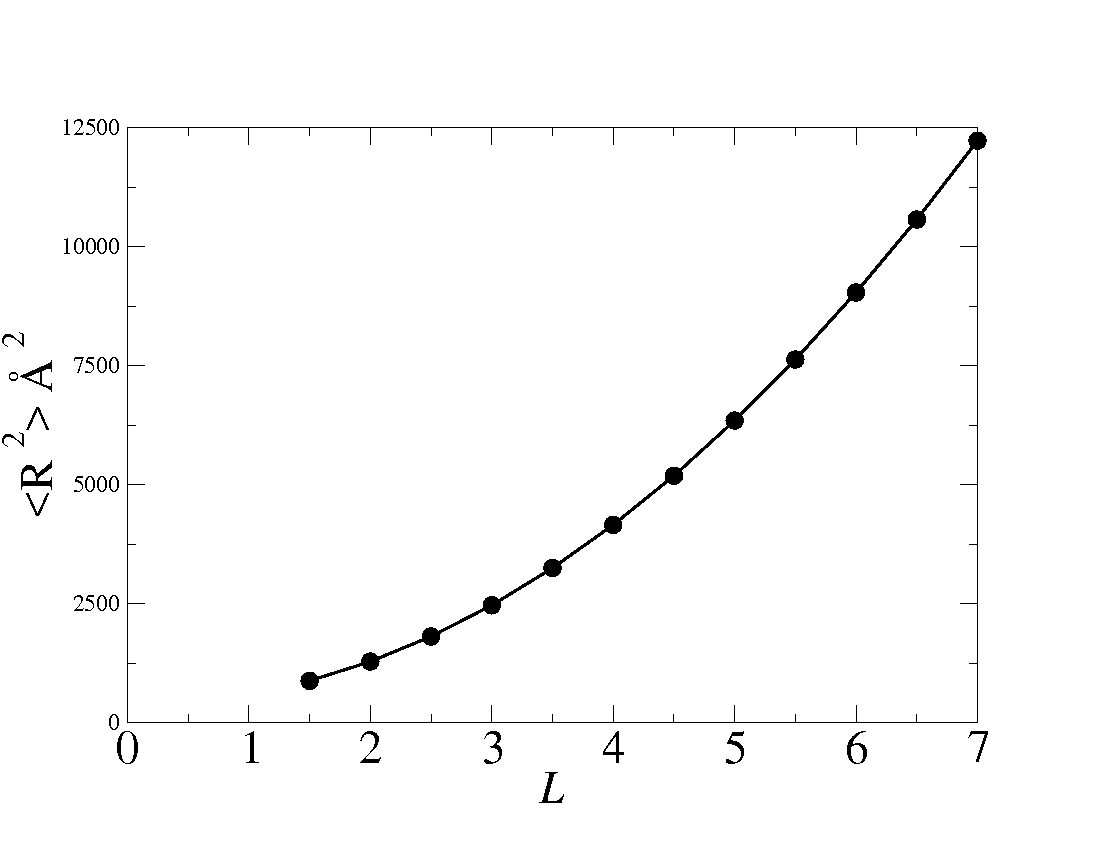
a b

Figure 6: (a) Mean square displacement $<R^{2}>$ as a function of $\cal L$. (b). FRET sensitized donor-to-acceptor intensity ratio ${\cal I}_{0}$ as a function of number of linker residues. Results presented are for data from experiments in the OFF or basal state from (1) Komatsu et al. (large filled green circles) and (2) Evers et al. (small filled green circles) superimposed on the theoretical predictions.

One of the striking features of panel (a) of Fig.2 in the main part of this paper was how easy it is to read off the binding energy corresponding to the experiment of Komatsu et al. (2011) by comparing their data with simulation. But in the ON state, the width $\Delta$ of the binding region as well as the depth $\epsilon$ can in principle influence the RET efficiency. To investigate this issue we have simply varied both parameters in the theoretical model, the results of which are given in Fig. 7. We see, as one might expect on theoretical grounds, that the signal to noise ratio has very little dependence on $\Delta$, which also is therefore the case for the RET efficiency (as the basal rate can have no such dependence).

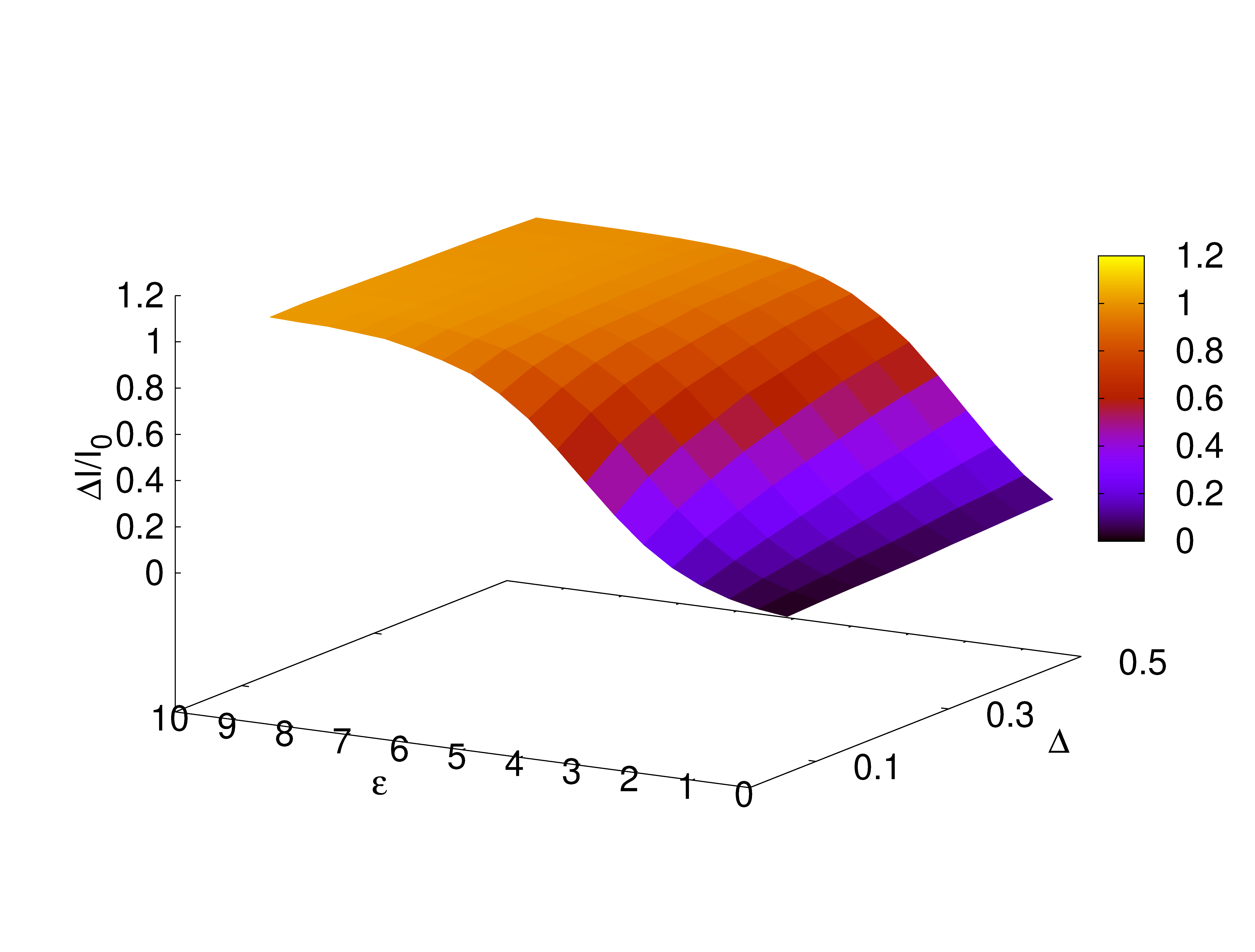
Figure 7: Dependence of the signal to noise ratio on the depth $\epsilon$ and width $\Delta$ of the attractive interaction (square well). While $\Delta{\cal I}/{\cal I}_{0}$ has a strong dependence on $\epsilon$, there is little dependence on $\Delta$.

Appendix B RET efficiency Observable and Sampling Procedure

The distance dependence of the FRET efficiency is approximated by the expression,

$${\cal I}(r)={1\over 1+(r/R_{0})^{6}}$$

with the Föster Radius $R_{0}\sim 5-7$ nm giving the distance at which the energy transfer efficiency is $50\%$ and $r$ is the distance between the spherical macro-particles. The expectation value of the RET efficiency $\overline{\cal I}$ can be calculated as an equilibrium average corresponding to the ON and OFF states respectively

$$\overline{\cal I}=\frac{\int dr{\cal I}(r)\exp(-\beta V(r))}{\int dr\exp(-\beta V(r))}$$

where the multidimensional nature of $r$ is implicit. $R_{0}$ depends on various quantities including fluorescence quantum yield of the donor in the absence of the acceptor, the refractive index of the medium, and the dipole orientation factor $<\kappa^{2}>$. The orientation dependence is given as ${R_{0}}^{6}\propto<\kappa^{2}>$, where $<\kappa^{2}>$ depends on the transition dipoles of the donor and acceptor fluorophores $\vec{D}$ and $\vec{A}$, and their mutual displacement $\vec{R}_{21}=\vec{R}_{2}-\vec{R}_{1}$,

$$\kappa=\vec{A}\cdot\vec{D}-\frac{3}{|\vec{R}_{21}|^{2}}\big{(}(\vec{D}\cdot\vec{R}_{21})(\vec{A}\cdot\vec{R}_{21})\big{)}$$ (5)

If the two fluorophores rotate freely one can show that $\overline{\kappa}^{2}=\frac{2}{3}$. This can be used to re-express the efficiency in terms of the rotationally averaged Föster radius $\overline{R_{0}}$ convenient for computation

$${\cal I}(r)={1\over 1+(r/\overline{R_{0}})^{6}\frac{2}{3}\frac{1}{<\kappa^{2}>}}$$ (6)

where the dependence of $\kappa$ on the transition dipoles and the mutual displacement of the fluorophores is implicit.

References

- Boersma et al. (2015) Boersma, A. J., Zuhorn, I. J., Poolman, B., 2015. A sensor for quantification of macromolecular crowding in living cell. Nat. Methods. 12 (3), 227–229.
- Corry et al. (2005) Corry, B., Jayatilaka, D., Rigby, P., 2005. A flexible approach to the calculation of resonance energy transfer efficiency between multiple donors and acceptors in complex geometries. Biophys. J. 89 (6), 3882–3836.
- Evers et al. (2006) Evers, T. H., v. Dongen, E. M., Faesen, A. C., Meijer, E. W., Merkx, M., 2006. Quantitative understanding of the energy transfer between fluorescent proteins connected via flexible peptide linkers. Biochemistry 45 (44), 13183–13192.
- Frenkel and Smit. (1996) Frenkel, D., Smit., B., 1996. Understanding Molecular Simulation: From Algorithms to Applications. Academic Press, Inc.
- Komatsu et al. (2011) Komatsu, N., Aoki, K., Yamadac, M., Yukinagac, H., Fujitac, Y., Kamioka, Y., , Matsuda, M., December 2011. Development of an optimized backbone of fret development of an optimized backbone of fret biosensors for kinases and gtpases. Mol. Biol. Cell. 22, 4647–4656.
- Lissandron et al. (2005) Lissandron, V., Terrin, A., Collini, M., D’alfonso, L., Chirico, G., Pantano, S., Zaccolo, M., 2005. Improvement of a fret-based indicator for camp by linker design and stabilization of donor-acceptor interaction. J. Mol. Biol. 354 (3), 546–555.
- Metropolis et al. (1953) Metropolis, N., Rosenbluth, A. W., Rosenbluth, M. N., Teller, A. H., Teller, E., 1953. Equation of state calculations by fast computing machines. J. Chem. Phys. 21 (6), 1087–1092.
- Sanyal et al. (2016) Sanyal, S., Coker, D. F., MacKernan, D., 2016. How flexible are flexible linkers in fret probes? Molecular Biosystems NA (NA), NA.
- Visser et al. (2003) Visser, N. V., Borst, J. W., van Hoek, A., Visser, A. J. W. G., 2003. Practical use of corrected fluorescence excitation and emission spectra of fluorescent proteins in förster resonance energy transfer (fret) studies. J. Fluorescence. 13 (3), 185–187.