Influence of intrinsic spin in the formation of singularities for inhomogeneous effective dust space-times

Abstract

The evolution of inhomogeneous space-times composed of uncharged fermions is studied for Szekeres metrics which have no Killing vectors, in general. Using the Einstein-Cartan theory to include the effects of (intrinsic) matter spin in General Relativity, the dynamics of a perfect fluid with non-null spin degrees of freedom is considered. It is shown that, if the matter is composed by effective dust and certain constraints on the initial data are verified, a singularity will not form. Various special cases are discussed, such as Lemaître-Tolman-Bondi and Bianchi $I$ space-times, where the results are further extended or shown explicitly to be verified.

I Introduction

It is known that the process of gravitational collapse in General Relativity (GR) can lead to spacetime singularities, which can correspond not only to black holes but also to naked singularities, depending on the initial data. In turn, the latter can challenge the cosmic censorship conjecture which, in this context, has been tested for various matter contents such as scalar fields sfcoll , perfect fluids pfcoll and imperfect fluids impflcoll .

It would then be interesting to explore alternative theories of gravity and test whether the results obtained within GR are robust with respect to small deviations from the theory. In particular, it is important to verify if corrections to GR may prevent the formation of singularities. Work along these lines has been done in alternative theories of gravity such as $F(R)$ gravity frcoll , Brans-Dicke theory BDcoll , Lovelock Lovecoll and Gauss-Bonnet gravity GBcoll , where it was found that the geometrical attributes absent in GR could affect the final fate of collapse.

In this paper, we consider the formalism provided by the Einstein-Cartan theory (ECT), where it is possible to introduce (intrinsic) spin degrees of freedom in a geometric theory of gravity. Such model is specially interesting because it encapsulates such quantum corrections in a semi-classical limit Hehl1 ; Hehl2 , providing a way to infer if quantum effects may avoid the formation of singularities.

Indeed, in the framework of loop quantum gravity, it was found that for a universe permeated by a scalar field, quantum corrections modify the classical Friedmann equation and a cosmological singularity can be avoided ashsingh ; quantumbounce . Moreover, some interesting but somewhat forgotten results from the 1970s Trautman ; Stewart ; Kop suggest that the introduction of spin in spatially homogeneous anisotropic models may prevent the formation of singularities, depending on the degree of isotropy of the collapsing space-time. However, in ref. Hehl1 , by applying the strong energy conditions to an effective energy-momentum tensor, it was shown that modified versions of the Hawking-Penrose singularity theorems hold, even considering the effects of spin.

More recently, the collapse process of a spatially homogeneous and isotropic spin fluid has been studied in astrosptor , where it was shown that there exists a competition between fluid and spin source parameters, so that the collapse end state is determined via the dynamics of these source terms and both singular and nonsingular solutions could be obtained. Moreover, the effects of spin have been shown to come into play in the cosmological context, where the torsion of space-time generated by spinning particles induces gravitational repulsion in fermionic matter in the early universe, where extremely high densities are present avoiding then the formation of space-time singularities Magueijo .

Nonetheless, spatially homogeneous and isotropic models may be seen as simplistic, so it would be interesting to explore this debate further by considering inhomogeneous and anisotropic space-times. Towards this goal, in this paper, we take a natural first step by considering effective inhomogeneous dust equations of state. This is surely a critical case which, yet, should be explored by comparison with the GR case, known to develop naked singularities.

We show that, with respect to the previous results, the situation can be more subtle: the effects of spin contribute, in a way, as a repulsive potential, therefore, collapsing solutions might not even exist for inhomegeneous space-times. Furthermore, even if some form of the energy conditions is verified, singularities may not be the end result of gravitational collapse if spin effects are considered.

The article is organized as follows: in Sec. II we include the effects of spin in the ECT and show that, in the considered setup, the resultant model is equivalent to an effective perfect fluid in the theory of GR; in Sec. III we consider the case of an effective dust fluid in a Szekeres space-time and study how the (intrinsic) spin degrees of freedom affect the evolution of the space-time and the formation of singularities; in Sec. IV we consider some particular solutions of the Szekeres model where previous results can be extended or shown to be verified explicitly; in Sec. V we summarize the results and conclude.

In this article all quantities are expressed in the geometrized unit system where $\mathcal{G}=c=1$, greek indices range from $0$ to $3$ and we use the metric signature $\left(-+++\right)$.

II Inclusion of spin effects in General Relativity

II.1 The Einstein-Cartan theory in brief

To include the spin effects in GR we shall follow the semi-classical approach provided by ECT and relate the spin of the matter fields with the space-time torsion tensor field. Now, let us briefly review the ECT and see how spin effects can be included in GR (for more details see e.g. Hehl1 ; Hehl2 ).

We start by recalling that, in this context, the covariant derivative of a vector field $U$ is given by

$$\nabla_{\alpha}U^{\beta}=\partial_{\alpha}U^{\beta}+C_{\alpha\sigma}^{\beta}U^{\sigma}\,,$$ (1)

constrained to be metric compatible, $\nabla_{\alpha}g_{\beta\gamma}=0$, but otherwise with a generic connection $C_{\alpha\beta}^{\gamma}$. The anti-symmetric part of the connection defines a tensor field, called the torsion tensor field,

$$S_{\alpha\beta}\,^{\gamma}\equiv C_{\left[\alpha\beta\right]}^{\gamma}=\frac{1}{2}\left(C_{\alpha\beta}^{\gamma}-C_{\beta\alpha}^{\gamma}\right)\,.$$ (2)

From this definition, it is possible to write the connection $C_{\alpha\beta}^{\gamma}$ as a combination of the torsion tensor plus the usual metric Christoffel symbols $\Gamma_{\alpha\beta}^{\gamma}$, such that $C_{\alpha\beta}^{\gamma}=\Gamma_{\alpha\beta}^{\gamma}+S_{\alpha\beta}\,^{\gamma}+S^{\gamma}\,_{\alpha\beta}-S_{\beta}\,^{\gamma}\,{}_{\alpha}$, or

$$C_{\alpha\beta}^{\gamma}=\Gamma_{\alpha\beta}^{\gamma}+K_{\alpha\beta}{}^{\gamma}\,,$$ (3)

where the tensor field,

$$K_{\alpha\beta}\,^{\gamma}\equiv S_{\alpha\beta}{}^{\gamma}+S^{\gamma}{}_{\alpha\beta}-S_{\beta}{}^{\gamma}{}_{\alpha}\,,$$ (4)

is called contorsion tensor.

Now, from the definition of the Riemann tensor

$$R_{\alpha\beta\gamma}{}^{\rho}=\partial_{\beta}C_{\alpha\gamma}^{\rho}-\partial_{\alpha}C_{\beta\gamma}^{\rho}+C_{\beta\sigma}^{\rho}C_{\alpha\gamma}^{\sigma}-C_{\alpha\sigma}^{\rho}C_{\beta\gamma}^{\sigma}\,,$$ (5)

and Eq. (3), we can write the Riemann tensor in ECT in terms of the metric Riemann tensor, $\widetilde{R}_{\alpha\beta\gamma}{}^{\rho}$, defined just in terms of the Christoffel symbols, and the contorsion tensor as

$$R_{\alpha\beta\gamma}{}^{\rho}=\widetilde{R}_{\alpha\beta\gamma}{}^{\rho}+2\widetilde{\nabla}_{\left[\beta\right.}K_{\left.\alpha\right]\gamma}{}^{\rho}+2K_{\left[\beta\right|\sigma}{}^{\rho}K_{\left|\alpha\right]\gamma}{}^{\sigma}\,,$$ (6)

where the square brackets denote anti-symmetrization in the indicated indexes and $\widetilde{\nabla}_{\alpha}$ represents the covariant derivative of a tensor quantity using only the metric connection $\Gamma_{\alpha\beta}^{\gamma}$. Contracting Eq. (6) gives the following expression for the Ricci tensor

$$R_{\alpha\gamma}=\widetilde{R}_{\alpha\gamma}+2\widetilde{\nabla}_{\left[\beta\right.}K_{\left.\alpha\right]\gamma}{}^{\beta}+2K_{\left[\beta\right|\sigma}{}^{\beta}K_{\left|\alpha\right]\gamma}{}^{\sigma}\,,$$ (7)

whereby the action for ECT which is linear with respect to curvature scalar can be written in the form

$$A=\frac{1}{16\pi}\int\sqrt{-g}\,g^{\alpha\gamma}\left\{\widetilde{R}_{\alpha\gamma}+K_{\beta\sigma}{}^{\beta}K_{\alpha\gamma}{}^{\sigma}-K_{\alpha\sigma}{}^{\beta}K_{\beta\gamma}{}^{\sigma}\right\}\,d^{4}x+\int\sqrt{-g}\,\mathcal{L}_{\text{Matter}}\,d^{4}x\,,$$ (8)

where $\mathcal{L}_{\text{Matter}}$ represents the matter Lagrangian density and we have omitted the total derivative terms. Following the Palatini approach, where the action is varied independently with respect to the space-time metric and the connection, we find two sets of field equations. Making the variation of the action in Eq. (8) with respect to the contorsion tensor we find

$$S^{\alpha\beta\mu}+2g^{\mu[\alpha}S^{\beta]}=-8\pi\Delta^{\alpha\beta\mu}\,,$$ (9)

where $S_{\alpha}\equiv S_{\mu\alpha}{}^{\alpha}$ and the quantity

$$\Delta^{\alpha\beta\mu}=\frac{1}{\sqrt{-g}}\frac{\delta\left(\sqrt{-g}\mathcal{L}_{\text{Matter}}\right)}{\delta K_{\mu\beta\alpha}}\,,$$ (10)

is usually called the intrinsic hypermomentum, as it encapsulates all the information of the microscopic structure of the matter that composes the fluid, i.e. intrinsic spin, dilaton charge and intrinsic shear. Notice that, in Eq. (9), the torsion tensor field is not a dynamical field, in the sense that the left hand side contains no derivatives of the torsion tensor and indeed appears as a purely algebraic equation. As such, in vacuum, where the matter Lagrangian density $\mathcal{L}_{\text{Matter}}$ is null, from Eq. (9), we see that the torsion tensor is effectively null so, all solutions of GR in vacuum are also solutions of ECT Hehl2 .

On the other hand, making the variation of the action in Eq. (8) with respect to the metric tensor we find the modified Einstein field equations

$$\widetilde{G}_{\mu\nu} -4S_{\sigma}K_{\mu\nu}{}^{\sigma}-2g^{\beta\delta}K_{\mu\sigma\delta}K_{\beta\nu}{}^{\sigma}+2g_{\mu\nu}S_{\sigma}S^{\sigma}+$$ (11)

$$+\frac{1}{2}g_{\mu\nu}K_{\rho\sigma\delta}K^{\delta\rho\sigma}-4S_{\mu}S_{\nu}-g^{\sigma\rho}K_{\beta\rho\nu}K_{\sigma\mu}{}^{\beta}=8\pi\,T_{\mu\nu}\,,$$

where $\widetilde{G}_{\mu\nu}\equiv\widetilde{R}_{\mu\nu}-\frac{1}{2}g_{\mu\nu}\widetilde{R}$ represents the Einstein tensor defined just using the metric connection, and

$$T_{\mu\nu}=g_{\mu\nu}\mathcal{L_{\text{Matter}}}-2\frac{\delta\mathcal{L}_{\text{Matter}}}{\delta g^{\mu\nu}}\,,$$ (12)

is the (symmetric) energy-momentum tensor of the matter fluid.

II.2 The Weyssenhoff fluid

To relate the torsion tensor field with the intrinsic spin of matter particles, we shall consider a perfect fluid with non-null (intrinsic) spin degrees of freedom that permeates a region of space-time. A description of such fluid is given by the Weyssenhoff model Weyssenhoff .

Although the Weyssenhoff fluid was first proposed as a phenomenological theory, a variational theory of an ideal spinning fluid has been developed Smalley ; obuk providing a Lagrangian for the Weyssenhoff semi-classical spin fluid which can, in turn, be used to compute the corresponding hypermomentum and energy-momentum tensors through Eqs. (10) and (12). It is then found that the Weyssenhoff fluid is characterized by the following relation between the intrinsic hypermomentum tensor and spin Smalley ; obuk

$$\Delta^{\mu\nu\alpha}=\frac{1}{2}\tau^{\mu\nu}u^{\alpha}\,,$$ (13)

where $u^{\alpha}$ is the fluid’s 4-velocity and $\tau^{\mu\nu}$ is an anti-symmetric tensor representing the spin density tensor which, in turn, verifies the following constraint

$$\tau^{\alpha\beta}u_{\beta}=0\,,$$ (14)

known as the Frenkel condition Frenkel1 ; Frenkel2 . Substituting Eqs. (13) and (14) in Eq. (9), we find that the torsion tensor is related to the intrinsic spin of matter as

$$S^{\alpha\beta\mu}=-4\pi\,\tau^{\alpha\beta}u^{\mu}\,,$$ (15)

making it clear that, in this model, spin constitutes the effective source of the torsion field. Eqs. (14) and (15) allow us then to rewrite Eq. (11) as

$$\widetilde{G}_{\mu\nu} +16\pi^{2}\tau_{\alpha\beta}\tau^{\alpha\beta}u_{\mu}u_{\nu}+8\pi^{2}g_{\mu\nu}\tau_{\alpha\beta}\tau^{\alpha\beta}$$ (16)

$$-32\pi^{2}\tau_{\mu\sigma}\tau_{\nu}{}^{\sigma}=8\pi\,T_{\mu\nu}\,.$$

Now, the spin tensor $\tau^{\mu\nu}$ and the energy-momentum tensor $T_{\mu\nu}$ that appear in Eqs. (13) - (16) refer to the spin and energy-momentum of microscopic particles. However, we are interested in studying the macroscopic behavior of an ideal spinning fluid. Therefore, to find the field equations that describe a macroscopic gravitational field due to a Weyssenhoff fluid, we have to compute a space-time average of the tensors $\tau^{\mu\nu}$ and $T_{\mu\nu}$ over an element of volume of the fluid, respectively $\langle\tau^{\mu\nu}\rangle$ and $\langle T_{\mu\nu}\rangle$.

Assuming that the spinning fluid is composed of microscopic particles with randomly oriented spin, we get the averaged quantities Gasperini

$$\langle\tau^{\mu\nu}\rangle =0\,,$$ (17)

$$\langle\tau^{\alpha\beta}\tau_{\alpha\beta}\rangle =2s^{2}\,,$$ (18)

$$\langle\tau_{\mu}{}^{\alpha}\tau_{\nu\alpha}\rangle =\frac{2}{3}\left(g_{\mu\nu}+u_{\mu}u_{\nu}\right)s^{2}\,,$$ (19)

where $s^{2}$ represents the average of the square of the spin density of the fluid. Moreover, from the Lagrangian density given in obuk for a zero-vorticity fluid, we find

$$\left\langle T_{\mu\nu}\right\rangle=-\frac{8\pi}{3}u_{\mu}u_{\nu}s^{2}-\frac{8\pi}{3}g_{\mu\nu}s^{2}+\left(\rho+p\right)u_{\mu}u_{\nu}+p\,g_{\mu\nu}\,,$$ (20)

where $\rho$ and $p$ represent the mass-energy density and pressure of the fluid, respectively. Substituting Eqs. (17) - (20) in the average version of Eq. (16) we find

$$\widetilde{G}_{\mu\nu}=8\pi\,\left[\left(\rho+p-4\pi s^{2}\right)u_{\mu}u_{\nu}+\left(p-2\pi s^{2}\right)\,g_{\mu\nu}\right]\,.$$ (21)

Notice that the field equations in Eq. (21), for a zero-vorticity Weyssenhoff fluid in the Einstein-Cartan theory, are actually equivalent to those in GR for a perfect fluid with additional contributions from the spin to the energy-density and pressure. Therefore, a spinning perfect fluid can be, classically, described by the theory of GR assuming that the fluid is described by the effective energy-momentum tensor

$$T_{\mu\nu}=\left(\rho_{\text{eff}}+p_{\text{eff}}\right)u_{\mu}u_{\nu}+p_{\text{eff}}\,g_{\mu\nu}\,,$$ (22)

with

$$\rho_{{\rm eff}}=\rho-2\pi s^{2}\qquad\text{and}\qquad p_{{\rm eff}}=p-2\pi s^{2},$$ (23)

where we have omitted the angular brackets. Nevertheless, one should bear in mind that all quantities are to be considered as averages.

Moreover, from now onwards, we will also omit the tilde to indicate tensor quantities computed only using the symmetric part of the connection since, as was shown, we can effectively treat the problem at hand using the theory of GR, where the torsion tensor is null.

II.3 The energy-momentum tensor for effective uncharged spinning dust

We shall now restrict our attention to the case where the fluid’s pressure varies in such a way that it cancels the contribution coming from spin effects, so that the whole fluid effectively behaves as dust, i.e.

$$p_{\text{eff}}=p-2\pi s^{2}=0\,.$$ (24)

so that

$$T_{\text{eff}}^{\mu\nu}=\rho_{\text{eff}}u^{\mu}u^{\nu}\,,$$ (25)

where $\rho_{\text{eff}}$ represents the effective mass-energy density of the matter.

Now, let us consider that the matter is composed of $N$ species of uncharged fermionic particles with mass $m_{i}$ and spin $s_{i}=\pm\hslash/2$ and assume that the interactions between the microscopic constituents of the fluid are negligible. Clearly, the distribution of spin and mass are related to each other. The particle number density for each species is given by Hehl1

$$n_{i}=\frac{\rho_{i}}{m_{i}}=\left(\frac{4s_{i}^{2}}{\hslash^{2}}\right)^{\frac{1}{2}}\,,$$ (26)

where $\rho_{i}$ and $s_{i}^{2}$ represent, respectively, the averaged energy density and the average of the squared spin density of a single species, such that

$$\rho_{i\text{eff}}=\rho_{i}-2\pi s_{i}^{2}\,,\qquad\text{and}\qquad\rho_{\text{eff}}=\sum_{i=1}^{N}\rho_{i\text{eff}}\,.$$ (27)

Using Eq. (26) in Eqs. (23) and (27) , we find that for each species

$$\rho_{i\text{eff}}=\rho_{i}\left(1-\frac{\rho_{i}}{\bar{\rho}_{i}}\right)\,,\qquad p_{i\text{eff}}=p_{i}-\frac{\rho_{i}^{2}}{\bar{\rho}_{i}}\,,$$ (28)

where the total pressure of the perfect fluid is formally given by

$$p_{\text{eff}}=\sum_{i=1}^{N}p_{i\text{eff}}\,,$$ (29)

and

$$\bar{\rho}_{i}=\frac{2m_{i}^{2}}{\pi\hslash^{2}}\,$$ (30)

represents a critical mass-density which sets a scale at which the spin effects have to be taken into account Hehl1 .

In the perfect fluid approximation, the various constituents of the matter are non-interacting. Therefore, the total pressure of the fluid will be null if the various terms in Eq. (29) are null. Substituting Eq. (28) in Eq. (24), we find that the constituents of the fluid are characterized by an equation of state of the form

$$p_{i}=\frac{1}{\bar{\rho}_{i}}\rho_{i}^{2}\,,$$ (31)

that is, a polytrope of order 2.

III Spin effects in the gravitational evolution

To study the influence of spin in singularity formation, we analyze the evolution of an uncharged effective dust fluid with non-null spin degrees of freedom composed only of fermionic particles.

When considering the case of the gravitational collapse of a compact object in astrophysics, we consider a model of Oppenheimer-Snyder type having a collapsing interior given by the Szekeres metric Szekeres1 ; Szekeres2 , which is inhomogeneous, matched to a vacuum exterior. Examples of such models were shown to exist in I_Brito ; Tod-Mena ; Bonnor . Whereas, when considering a cosmological model, we shall assume that the coordinates in the Szekeres metric are globally defined and that the universe can either initially be expanding or contracting. In this case, part of the problem will be to figure out if, during evolution, there can be a bounce in the collapsing phase or a turning point, followed by recollapse, in the expanding phase.

The Szekeres space-time represents the solutions of the Einstein field equations (EFE) for a space-time permeated by irrotational dust whose line element can be written in the form

$$ds^{2}=-d\tau^{2}+e^{\alpha\left(\tau,r,p,q\right)}dr^{2}+e^{\beta\left(\tau,r,p,q\right)}\left(dp^{2}+dq^{2}\right)\,,$$ (32)

where $\alpha$ and $\beta$ are $C^{2}$-functions of the coordinates $\tau,r,p,q$. This metric has no Killing vectors, in general Bonnor-2 . Historically, the Szekeres models are split in two classes: one that generalizes the Lemaître-Tolman-Bondi (LTB) metrics and another that generalizes the Kantowski-Sachs (KS) metrics. We shall treat them separately.

III.1 Szekeres space-times: LTB-like

The LTB-like Szekeres models are characterized by a line element of the form Szekeres1 ; Szekeres2

$$ds^{2}=-d\tau^{2}+\frac{\left(R^{\prime}-\frac{RE^{\prime}}{E}\right)^{2}}{\epsilon+f\left(r\right)}dr^{2}+\frac{R^{2}}{E^{2}}\left(dp^{2}+dq^{2}\right)\,,$$ (33)

where the prime indicates a derivative with respect to $r$ , $\epsilon=\left\{-1,0,1\right\}$, $E=E\left(r,p,q\right)$ and $f\left(r\right)$ are arbitrary $C^{2}$ functions such that $f\left(r\right)+\epsilon>0$, while the function $R=R\left(\tau,r\right)$ satisfies the Friedmann like equation

$$\dot{R}^{2}\left(\tau,r\right)=f\left(r\right)+\frac{2M\left(r\right)}{R\left(\tau,r\right)}\,,$$ (34)

with the overdot denoting a derivative with respect to the time coordinate $\tau$ and $M=M\left(r\right)$ is another arbitrary function.

Given the line element in Eq. (33) and Eq. (25) we find, from the EFE, the following relation between the mass-energy density of the effective dust source and the functions that describe the geometry of the space-time

$$8\pi\,\rho_{\text{eff}}=2\frac{EM^{\prime}-3ME^{\prime}}{R^{2}\left(ER^{\prime}-RE^{\prime}\right)}\,.$$ (35)

This expression can be re-written as

$$\rho_{\text{eff}}\left(\tau,r,p,q\right) =\frac{r^{2}\,F\left(r,p,q\right)}{R^{2}\left(\tau,r\right)W\left(\tau,r,p,q\right)}\,,$$ (36)

where

$$r^{2}F\left(r,p,q\right)=\frac{1}{4\pi}\left[E\left(r,p,q\right)M^{\prime}\left(r\right)-3M\left(r\right)E^{\prime}\left(r,p,q\right)\right]\,,$$ (37)

and

$$W\left(\tau,r,p,q\right)=E\left(r,p,q\right)R^{\prime}\left(\tau,r\right)-R\left(\tau,r\right)E^{\prime}\left(r,p,q\right)\,,$$ (38)

so, $f\left(r\right)$, $M\left(r\right)$ and $E\left(r,p,q\right)$ will be free initial functions that characterize the space-time. In turn, $E\left(r,p,q\right)$ is written in terms of another 3 free functions (see Szekeres1 ; Szekeres2 ), but we will not have to use this fact in the what follows.

III.1.1 Regularity conditions and the influence of spin in singularity formation

Since we are interested in studying the influence of spin in the formation of curvature singularities, in addition to the previous assumptions we shall consider some further requirements on the initial regularity of the space-time:

Assumption 1.

At the initial time $\tau=\tau_{0}$:

1. $R\left(\tau_{0},r\right)$ is an increasing function of the coordinate $r$.

2. The space-time is non-singular.

3. For every triplet $(r,p,q)$, we assume $W\left(\tau_{0},r,p,q\right)$ and $\rho_{\text{eff}}\left(\tau_{0},r,p,q\right)$ to be non-null.

Under these assumptions, we can set by convention

$$R\left(\tau_{0},r\right)=r.\,$$ (39)

When it exists, it is also useful to introduce $\tau_{c}\left(r\right)>\tau_{0}$, defined as the value of the time coordinate at which the function $R$ of the shell with coordinate $r$ goes to zero.

Under our assumptions, from Eqs. (36), and in the coordinate system defined by Eq. (39), it is straightforward to see that the function $F\left(r,p,q\right)$ must be finite and non-null. This leads us to conclude that a necessary condition for the divergence of $\rho_{\text{eff}}\left(\tau,r,p,q\right)$ for a given $\left(r,p,q\right)$ is that either $R\left(\tau,r\right)$ or $W\left(\tau,r,p,q\right)$ go to zero at some instant of time $\tau_{S}>\tau_{0}$. The former is associated with a shell-focusing singularity, whereas the latter represents the formation of a shell-crossing singularity Szekeres .

Moreover, since the functions $R\left(\tau,r\right)$ and $W\left(\tau,r,p,q\right)$ are continuous in the time coordinate $\tau$ before the singularity formation, for each triad $\left(r,p,q\right)$, the effective mass-energy density function $\rho_{\text{eff}}\left(\tau,r,p,q\right)$ is also a continuous function in the coordinate $\tau$. We are then able to prove

Lemma 1.

Under our assumptions if, in a continuous gravitational collapse, there exists a curve $\tau=\tau_{s}(r)>\tau_{0}$ such that for each $(r,p,q)$ within the matter, either $\lim_{\tau\to\tau_{s}(r)^{-}}R\left(\tau,r\right)=0$ or $\lim_{\tau\to\tau_{s}(r)^{-}}W\left(\tau,r,p,q\right)=0$ then, $\lim_{\tau\to\tau_{s}(r)^{-}}\rho_{\text{eff}}\left(\tau,r,p,q\right)=-\infty$.

Proof.

We split the proof in two parts:

1. First, we prove that for each triad $\left(r,p,q\right)$, if either $\lim_{\tau\to\tau_{s}(r)^{-}}R\left(\tau,r\right)\to 0$ or $\lim_{\tau\to\tau_{s}(r)^{-}}W\left(\tau,r,p,q\right)\to 0$ for some instant $\tau_{s}>\tau_{0}$, then we have that $\lim_{\tau\to\tau_{s}(r)^{-}}\rho_{\text{eff}}\left(\tau,r,p,q\right)\to\pm\infty$. As was discussed previously, a necessary condition for divergent $\rho_{\text{eff}}$ is that either $W\left(\tau,r,p,q\right)$ or $R\left(\tau,r\right)$ go to zero at some instant $\tau=\tau_{s}$. In appendix A it is shown that if $R$ is a real function, these conditions are also sufficient for the divergence of $\rho_{\text{eff}}$, in particular, even in the case where $\lim_{\tau\to\tau_{s}(r)^{-}}W\to\infty$, the limit $\lim_{\tau\to\tau_{s}(r)^{-}}R^{2}R^{\prime}\to 0$ is always verified, hence from (38) $\lim_{\tau\to\tau_{s}(r)^{-}}R^{2}W\to 0$ and from (36) $\lim_{\tau\to\tau_{s}(r)^{-}}\rho_{\text{eff}}\left(\tau,r,p,q\right)\to\pm\infty$, as $F(r,p,q)$ is finite. Therefore, since $F\left(r,p,q\right)$ takes finite values, from Eq. (36), fixing $(r,p,q)$, if either $\lim_{\tau\to\tau_{s}(r)^{-}}R\left(\tau,r\right)\to 0$ or $\lim_{\tau\to\tau_{s}(r)^{-}}W\left(\tau,r,p,q\right)\to 0$ for some instant $\tau_{s}>\tau_{0}$, then we have $\lim_{\tau\to\tau_{s}(r)^{-}}\rho_{\text{eff}}\left(\tau,r,p,q\right)\to\pm\infty$.

2. We now show that we can only have $\rho_{\text{eff}}\left(\tau,r,p,q\right)\to-\infty$. For a dust spacetime composed only of fermions, the effective mass-energy density is given by the sum in Eq. (27) and it takes infinite values if, at least, one term of the sum, $\rho_{i\text{eff}}$, is infinite. Although we shall restrain ourselves from imposing any of the usual energy conditions, we shall consider that if any of the parameters that characterize the fluid take complex values at any point of the space-time, the solution is unphysical. Therefore, for $\rho_{i}\in\mathbb{R}\setminus\{0\}$, from Eq. (28), we find that each $\rho_{i\text{eff}}$ may only tend to $-\infty$, hence, for each $(r,p,q)$, $\lim_{\tau\to\tau_{s}(r)^{-}}\rho_{\text{eff}}\left(\tau,r,p,q\right)\to-\infty$. ∎

Now, from Lemma 1, we get the following result:

Theorem 1.

Given a Szekeres space-time with line element (33) permeated by an uncharged perfect fluid composed only of fermionic particles, characterized by an equation of state such that, the fluid effectively behaves as dust, if Assumption 1 is verified and $\text{sign}\left(F\left(r,p,q\right)\right)=\text{sign}\left(W\left(\tau_{0},r,p,q\right)\right)$ then, a curvature singularity will not form.

Proof.

The proof follows from Lemma 1 and the continuity of $R$, $W$ and $\rho_{eff}$.

Consider that $\text{sign}\left(F\left(r,p,q\right)\right)=\text{sign}\left(W\left(\tau_{0},r,p,q\right)\right)$.

Let us start by showing that the function $W\left(\tau,r,p,q\right)$ will not be zero for any $\tau\in\left]\tau_{0},\tau_{c}\left(r\right)\right]$. We argue by contradiction.

Assume that there exists, for each $r$, an instant $\tau_{1}\left(r\right)\in\left]\tau_{0},\tau_{c}\left(r\right)\right]$ such that $\lim_{\tau\to\tau_{1}^{-}}W\left(\tau_{1},r,p,q\right)=0$. Then, from Lemma 1, $\lim_{\tau\to\tau_{1}^{-}}\rho_{\text{eff}}\left(\tau,r,p,q\right)\to-\infty$. From our assumptions, $W\left(\tau,r,p,q\right)$ and $R\left(\tau,r\right)$ are continuous functions in the $\tau$ coordinate for all $\tau\in\left]\tau_{0},\tau_{1}\right[$ therefore, the effective mass-energy density, $\rho_{\text{eff}}$, is a continuous function in the coordinate $\tau$ for all $\tau_{2}<\tau_{1}$, concluding that $\rho_{\text{eff}}\left(\tau_{2},r,p,q\right)<0$. On the other hand, continuity of $W\left(\tau,r,p,q\right)$ implies that the sign of $W\left(\tau_{2},r,p,q\right)$ must be equal to the sign of $W\left(\tau_{0},r,p,q\right)$. Therefore, since $R\left(\tau_{2},r\right)>0$ and $\text{sign}\left(F\left(r,p,q\right)\right)=\text{sign}\left(W\left(\tau_{2},r,p,q\right)\right)$, we conclude, from Eq. (36), $\rho_{\text{eff}}\left(\tau_{2},r,p,q\right)>0$, contradicting what was shown before. Hence, $W\left(\tau,r,p,q\right)$ will not be zero for any $\tau\in\left]\tau_{0},\tau_{c}\left(r\right)\right]$.

The case when the function $R\left(\tau,r\right)$ goes to zero before the function $W\left(\tau,r,p,q\right)$ also can not occur since, from Eq. (36), Lemma 1 would be violated. ∎

Remark 1.

The condition $\text{sign}\left(F\left(r,p,q\right)\right)=\text{sign}\left(W\left(\tau_{0},r,p,q\right)\right)$ of Theorem 1 is equivalent to consider that the effective energy-momentum tensor (25) verifies the weak energy condition at the initial time $\tau_{0}$.

Remark 2.

To clarify the statement of the Theorem 1, let us consider the simpler case of an effective dust fluid composed of only one type of fermions. In this case, from Eqs. (28) and (36) we can solve for $\rho$, such that

$$\rho\left(r,p,q\right)=\frac{\bar{\rho}}{2}\left(1\pm\sqrt{1-\frac{4r^{2}F}{\bar{\rho}R^{2}W}}\right)\,,$$ (40)

hence, given $\text{sign}\left(F\left(r,p,q\right)\right)=\text{sign}\left(W\left(\tau_{0},r,p,q\right)\right)$, from the results of Appendix A, if, for each $r$, either $W\left(\tau,r,p,q\right)$ or $R\left(\tau,r\right)$ go to zero for some instant $\tau\in\left]\tau_{0},\tau_{c}\left(r\right)\right]$, the energy density profile for the fluid will take complex values, hence considered unphysical.

III.2 Szekeres space-times: KS-like

The KS-like Szekeres models are characterized by the general line element Szekeres1

$$ds^{2}=-d\tau^{2}+\left[X\left(\tau,r\right)-R\left(\tau\right)\frac{E_{1}\left(r,p,q\right)}{E_{0}\left(p,q\right)}\right]^{2}dr^{2}+\frac{R\left(\tau\right)^{2}}{E_{0}\left(p,q\right)^{2}}\left(dp^{2}+dq^{2}\right)\,,$$ (41)

where the function $R\left(\tau\right)$ verifies

$$\dot{R}\left(\tau\right)^{2}=\frac{2M}{R\left(\tau\right)}+k_{1}\,,$$ (42)

with $M$ being an arbitrary constant to be given as initial data and the constant $k_{1}$ is determined by

$$\left(\partial_{p}E_{0}\right)^{2}+\left(\partial_{q}E_{0}\right)^{2}-E_{0}\left(\partial_{p}^{2}E_{0}+\partial_{q}^{2}E_{0}\right)=k_{1}\,.$$ (43)

Moreover, the function $X\left(\tau,r\right)$ is a solution of following equation:

$$X\,\ddot{R}+\dot{R}\,\dot{X}+R\,\ddot{X}=\frac{k_{2}\left(r\right)}{2}\,,$$ (44)

with

$$2\partial_{q}E_{0}\partial_{q}E_{1}+2\partial_{p}E_{0}\partial_{p}E_{1}-\left(\partial_{q}^{2}E_{0}+\partial_{p}^{2}E_{0}\right)E_{1}-E_{0}\left(\partial_{p}^{2}E_{1}+\partial_{q}^{2}E_{1}\right)=k_{2}(r)\,,$$ (45)

where we have omitted some functional dependencies to avoid saturating the notation.

From the EFE, the effective mass-energy density of the spinning cloud verifies

$$\rho_{\text{eff}}=\frac{G\left(r,p,q\right)}{R^{2}\left(\tau\right)H\left(\tau,r,p,q\right)}\,,$$ (46)

where

$$H\left(\tau,r,p,q\right)=X\left(\tau,r\right)\,E_{0}\left(p,q\right)-R\left(\tau\right)\,E_{1}\left(r,p,q\right)\,.$$ (47)

Such space-times are completely determined by the initial functions $E_{0}\left(p,q\right)$and $E_{1}\left(r,p,q\right)$ and the constant $M$.

III.2.1 Regularity conditions and the influence of spin in singularity formation

As in the previous section, we shall consider some further constraints on the initial regularity of the space-time:

Assumption 2.

1. At the initial time, $\tau=\tau_{0}$, the space-time is non-singular.

2. For every triplet $(r,p,q)$, we assume $H\left(\tau_{0},r,p,q\right)$ and $\rho_{\text{eff}}\left(\tau_{0},r,p,q\right)$ to be non-null.

Now, given the above initial regularity constraints and looking at Eqs. (46) and (47), as well as to the solutions in Appendix A, it can be seen that, following the same reasoning applied in the proofs of subsection III.1.1, we have the following result:

Proposition 1.

Given a Szekeres space-time with line element (41) filled with an uncharged perfect fluid composed only of fermionic particles, characterized by an equation of state such that, the fluid effectively behaves as dust, if assumptions 2 are verified and $\text{sign}\left(G\left(r,p,q\right)\right)=\text{sign}\left(H\left(\tau_{0},r,p,q\right)\right)$, then a curvature singularity will not form.

IV Special Cases

In this section, we shall discuss the effects of spin in the formation of singularities for some particular cases of the Szekeres space-times, where the analysis of the previous section can be extended.

IV.1 Lemaître-Tolman-Bondi space-time

The Lemaître-Tolman-Bondi (LTB) space-time is a solution of the EFE for a spherically symmetric neutral dust source characterized, in co-moving coordinates, by the line element

$$ds^{2}=-d\tau^{2}+\frac{R^{\prime}\left(\tau,r\right)^{2}}{1+f\left(r\right)}dr^{2}+R\left(\tau,r\right)^{2}d\Omega^{2}\,,$$ (48)

where $d\Omega^{2}\equiv d\theta^{2}+\sin^{2}\theta\,d\varphi^{2}$ represents the line element of the unit 2-sphere. The function $R\left(\tau,r\right)$ verifies Eq. (34) and represents the circumference radius at an instant $\tau$ and radial coordinate $r$ and $f\left(r\right)>-1$ is an arbitrary $C^{2}$-function of the radial coordinate. The LTB metric can be found from the Szekeres solution, Eq. (33), by setting $E^{2}\left(r,p,q\right)=\left(1+p^{2}+q^{2}\right)/4$ and $\epsilon=1$.

From the EFE, we find that Eq. (36) is re-written for the LTB space-time as

$$\rho_{\text{eff}}\left(\tau,r\right) =\frac{r^{2}\,F\left(r\right)}{R^{2}R^{\prime}}\,,$$ (49)

where $F\left(r\right)$ is another arbitary function of $r$ and it is related to the function $M\left(r\right)$, Eq. (34), by $M^{\prime}\left(r\right)=4\pi r^{2}\,F\left(r\right)$, or

$$M\left(r\right)=4\pi\int_{0}^{r}F\left(\mathrm{r}\right)\,\mathrm{r}^{2}\,d\mathrm{r}.$$ (50)

It is worth remarking that, in this case, the function $M\left(r\right)$ represents the mass contained within a shell with coordinate $r$ (see e.g. Landau ).

In the case of a LTB space-time, the function $W\left(\tau,r\right)\equiv R^{\prime}\left(\tau,r\right)$ and in the coordinate system defined by Eq. (39) we have $W\left(\tau_{0},r\right)=+1$. Therefore, for the LTB space-time imposing $F\left(r\right)>0$ is equivalent to impose $M^{\prime}\left(r\right)>0$.

The result in Theorem 1, albeit important, does not provide an answer in the cases where $F\left(r\right)<0$. One might think that such cases are unphysical since the effective energy conditions would be violated. There are, however, known physical phenomena that seem to violate the energy conditions (see e.g. Visser ). Moreover, cases of collapsing space-times with negative mass have been studied several times in the past (see e.g. RMann ; Bubble and references therein).

Let us then consider that $M^{\prime}\left(r\right)$ takes negative values for all $r$. In this case we have, from Eq. (50), that the mass function $M\left(r\right)$ is negative for all $r$. Assuming that $f\left(r\right)\geq-2M/r$, otherwise Eq. (34) has no real solutions, it is clear, from Eq. (34), that one of two scenarios will occur: either $\dot{R}\left(\tau_{0},r\right)>0$, in which case the effective dust matter will continue to expand indefinitely; or $\dot{R}\left(\tau_{0},r\right)<0$ where at some instant of time, say $\tau_{b}$, $\dot{R}\left(\tau_{b},r\right)$ will go to zero. From Eq. (34), it is easy to show that $\ddot{R}(\tau,r)$ is always positive, therefore, at $\tau_{b}$, the function $R$ will have a minimum. Hence, the system will bounce back and start to expand indefinitely.

We summarize these conclusions in the next proposition, which softens the conditions of Theorem 1 for the case of LTB:

Proposition 2.

Given a LTB space-time composed of a spherically symmetric, uncharged, collapsing perfect fluid, composed only of fermionic particles, characterized by an equation of state such that, the fluid effectively behaves as dust, if Assumptions 1 are verified and $\text{sign}\left(M^{\prime}\left(r\right)\right)$ is the same for all $r$ within the space-time, the circumferential radius function $R\left(\tau,r\right)$ will not go to zero.

Aside the simpler case where $M^{\prime}\left(r\right)<0$ for all $r$, there may be configurations where there are regions of the space-time with positive effective energy density and other regions with negative effective energy density, however, it is easy to show that such configurations are solutions of the Einstein field equations only if surface layers, separating the different regions, are present. Such cases shall not be considered here.

To conclude this subsection, we note that if $M^{\prime}\left(r\right)$ takes negative values, shell-crossing singularities may occur.

IV.1.1 The evolution of the collapse

In the previous subsection it was shown that, under our assumptions, and if the sign of the function $M^{\prime}\left(r\right)$ is the same for all $r$, an uncharged effective dust cloud composed only of fermionic particles, in a LTB space-time will not form a shell-focusing singularity. Then, for $\dot{R}(\tau_{0},r)<0$, and assuming that no shell-crossing singularities occur for $\text{sign}\left(M^{\prime}(r)\right)<0$, there are only three possibilities for the behavior of the uncharged effective dust cloud:

1. there are no global in time solutions of the EFE for a collapsing uncharged effective dust matter;

2. the gravitational collapse will lead to a bounce of the matter cloud;

3. the gravitational collapse of the matter cloud will settle in a stable configuration.

As we shall see below, the third scenario will never occur, and the first and second cases may occur depending on the initial data:

(I) Consider the initial data $M\left(r\right)>0$ and $f\left(r\right)\geq 0$ or $M\left(r\right)=0$ and $f\left(r\right)>0$. In both cases, from Eq. (34), the function $\dot{R}$ can not go to zero, that is, for a given $r$, $R\left(\tau,r\right)$ is either a strictly decreasing or a strictly increasing function of $\tau$. However, if $R$ is a decreasing function in the $\tau$ coordinate, it will eventually go to zero, violating the result of Proposition 2. Hence, in these cases, the only possible physical solution is when the matter expands indefinitely.

(II) Another possibility is the case where $M\left(r\right)<0$ and $f\left(r\right)>0$, with $2M\left(r\right)/R\left(\tau_{0},r\right)+f\left(r\right)>0$ for a given $r$ within the matter cloud. In this case, from Eq. (34), there are two possible behaviors depending on the initial value of $\dot{R}\left(\tau\right)$: either $\dot{R}\left(\tau_{0},r\right)>0$, in which case the effective dust cloud will continue to expand indefinitely; or $\dot{R}\left(\tau_{0},r\right)<0$, where at some instant of time, $\tau_{b}$, $\dot{R}\left(\tau_{b},r\right)$ will go to zero. From Eq. (34), it is easy to show that $\ddot{R}(\tau,r)$ is always positive. Therefore, at $\tau_{b}$, the function $R$ will attain a minimum, different from zero, concluding that the system will bounce and start to expand from then on. Note that this solution is characterized by $M\left(r\right)<0$, therefore the weak energy condition is not verified and there is no inconsistency with the result in ref. Hehl1 .

(III) Yet another possibility is the case where $M\left(r\right)>0$ and $f\left(r\right)<0$, with $2M\left(r\right)/R\left(\tau_{0},r\right)+f\left(r\right)>0$: if initially $\dot{R}\left(\tau_{0},r\right)<0$, then a singularity will eventually form; on the other hand, if $\dot{R}\left(\tau_{0},r\right)>0$, $\dot{R}$ will go to zero at some $\tau\in]\tau_{0},+\infty[$, however, from Eq. (34) we see that $\ddot{R}(\tau,r)$ is always negative in this case, hence, the system will cease to expand further and start to collapse, eventually forming a singularity. In both scenarios the result in Theorem 1 is violated, hence, such initial data does not correspond to a physical solution. This is because $M\left(r\right)>0$ implies that at some region $F\left(r\right)>0$, therefore, if a singularity occurs the energy density of the constituents of the fluid would have to take complex values.

As examples, in Figs. 1 and 2, we show the behavior of $R$ as a function of $\tau$ for various fixed values of the coordinate $r$, depending on the initial sign of $\dot{R}\left(\tau_{0},r\right)$, found by numerically solving Eq. (34) in particular cases when $M\left(r\right)<0$ and $f\left(r\right)>0$ and $M\left(r\right)>0$ and $f\left(r\right)<0$, respectively.

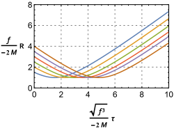
(a)

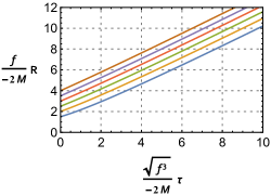
(b)

Figure 1: Behavior of the function $R\left(\tau,r\right)$ for various fixed values of the coordinate $r$, depending on the initial value of $\dot{R}$, in the case of $M\left(r\right)<0$ and $f\left(r\right)>0$. Panel a) At the initial time $\dot{R}\left(\tau_{0},r\right)<0$. Panel b) At the initial time $\dot{R}\left(\tau_{0},r\right)>0$.

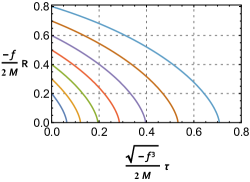
(a)

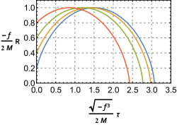
(b)

Figure 2: Behavior of the function $R\left(\tau,r\right)$ for various values of the coordinate $r$ depending of the initial value of $\dot{R}$ in the case of $M\left(r\right)>0$ and $f\left(r\right)<0$. Panel a) At the initial time $\dot{R}\left(\tau_{0},r\right)<0$. Panel b) At the initial time $\dot{R}\left(\tau_{0},r\right)>0$.

IV.2 Friedmann-Lemaître-Robertson-Walker space-time

Another example of notable interest is the Friedmann-Lemaître-Robertson-Walker (FLRW) model, where the space-time is parametrized by a spherically symmetric spatially homogeneous and isotropic dust metric, such that

$$ds^{2}=-d\tau^{2}+a\left(\tau\right)^{2}\left(\frac{dr^{2}}{1+k\,r^{2}}+r^{2}d\Omega^{2}\right)\,,$$ (51)

where $a\left(\tau\right)$ is the scale factor and $k=\left\{-1,0,1\right\}$. This solution is a particular case of the Szekeres line element, Eq. (33), by setting $E^{2}\left(r,p,q\right)=\left(1+p^{2}+q^{2}\right)/4$, $\epsilon=1$, $f\left(r\right)\equiv k\,r^{2}$ and $R\left(\tau,r\right)\equiv a\left(\tau\right)r$. We then have for an effective dust cloud

$$\rho_{\text{eff}}\left(\tau\right)=\frac{F_{0}}{a^{3}\left(\tau\right)}\,,$$ (52)

with $F_{0}$ being a non-zero constant, and $a\left(\tau\right)$ satisfying the well-known Friedmann equation

$$\dot{a}^{2}\left(\tau\right)=\frac{2M(r)}{r^{3}\,a\left(\tau\right)}+k\,,$$ (53)

where

$$M(r)=M_{0}r^{3},\qquad\text{ with }\leavevmode\nobreak\ \leavevmode\nobreak\ \leavevmode\nobreak\ M_{0}=\frac{4\pi}{3}F_{0}=\frac{4\pi}{3}a\left(\tau_{0}\right)^{3}\rho_{\text{eff}}\left(\tau_{0}\right)\,.$$ (54)

Moreover, this space-time is itself a particular case of the LTB space-time studied in the previous subsection. Therefore, all the previous results are valid for this particular case.

From Proposition 2 we know that independently of the sign of $M_{0}$, or equivalently $F_{0}$, a singularity does not occur. As discussed in subsection IV.1.1, the actual evolution of space-time depends of the values of the constants $k$ and $M_{0}$. More concretely,

1. for $M_{0}>0\wedge k\geq 0$, the space-time will expand indefinitely;

2. for $M_{0}<0\wedge k>0$, depending on whether $\dot{a}\left(\tau_{0}\right)>0$ or $\dot{a}\left(\tau_{0}\right)<0$, the space-time will either expand indefinitely or start by a collapsing phase which is followed by a nonsingular bounce and then entering an expanding phase, respectively;

in all other cases, from Eq. (53), we find that the functions $a\left(\tau\right)$ or $\rho\left(\tau\right)$ will take complex values, hence, the solutions to the Friedmann equations are considered unphysical (see also Sec.6.2 of ref. Griff_Podolsky ).

By comparison with our setup, we recall that in ref. Trautman , the effects of spin in singularity formation was studied by considering a dust cloud composed of fermionic particles in a FLRW space-time whose spins were assumed to be aligned in a given preferred spatial direction. In that case, the field equations can be explicitly solved and a closed form expression for the scale factor $a\left(\tau\right)$ was found, showing explicitly that there is a minimum positive value for $a\left(\tau\right)$ thus, concluding that a singularity does not form. Moreover, cosmological as well as astrophysical consequences of introducing spin and torsion in gravitation has been studied in cosmosptor and astrosptor ; astrosptor1 , respectively. In the former, a closed homogeneous and isotropic universe filled with fermionic matter has been considered and it was shown that the effects of spin-torsion coupling produces a gravitational repulsion in the early universe, preventing the formation of cosmological singularity. In the latter papers, the effects of spin on the dynamics of collapse for a closed astrosptor and flat astrosptor1 FLRW backgrounds has been studied. It was shown that, under certain conditions, the formation of space-time singularities can be avoided through a non-singular bounce, which can either be hidden behind a horizon or visible to external observers, depending on the initial radius or mass of the collapsing body.

All the previous mentioned cases differ from our setup since we assume that spins are randomly oriented and the fluid effectively behaves as dust. However, as was shown above, our conclusions are similar.

IV.3 Senovilla-Vera space-time

As a special inhomogeneous case of KS-like Szekeres space-times, we study the Senovilla-Vera space-time Senovilla characterized by a line element of the form

$$ds^{2}=-d\tau^{2}+dr^{2}+r^{2}d\varphi^{2}+\left(\beta+\frac{\tau^{2}+r^{2}}{\gamma}\right)^{2}dz^{2}\,,$$ (55)

where $\gamma\in\mathbb{R}\backslash\left\{0\right\}$, $\beta\in\mathbb{R}_{\geq 0}$, $r>0$, $z\in\left]-\infty,+\infty\right[$ and $\varphi\in\left[0,2\pi\right[$. A space-time exterior to (55) was found in I_Brito . Assuming that the space-time is permeated by effective dust, we find that the effective mass-energy density is given by

$$8\pi\rho_{\text{eff}}\left(\tau,r\right)=-\frac{4}{\beta\gamma+r^{2}+\tau^{2}}\,.$$ (56)

In the cases where $\gamma>0\wedge\beta\geq 0$ or $\gamma<0\wedge\gamma\beta+r^{2}>0$, it is clear that there are no collapsing solutions. Let us then consider the cases where $\gamma<0\wedge\gamma\beta+r^{2}<0$. Setting $R=1$, $E_{0}=1$, $X=\tau^{2}/\gamma$ and $E_{1}=-\left(r^{2}+\beta\gamma\right)/\gamma$ in Eq. (41), we recover the line element (55). The functions $G$ and $H$, in Eqs. (46) and (47), are in this case

$$H\left(\tau,r\right)=\beta+\frac{\tau^{2}+r^{2}}{\gamma}\,,\qquad\qquad G=-\frac{1}{2\pi\gamma}\,.$$ (57)

Now, for $\gamma<0$ we see that the function $H\left(\tau,r\right)$ is a strictly decreasing function of the coordinate $\tau$. It is then clear that, for $\gamma\beta+r^{2}<0$, such model is not a solution of the EFE for effective dust, since this would imply the formation of a curvature singularity when $\tau=\sqrt{\gamma\beta+r^{2}}$, violating Proposition 1.

We can see this more clearly by considering that the fluid is composed of only one type of fermionic particles. In that case, from Eqs. (28) and (56) we have that the mass-energy density of the perfect fluid is given by

$$\rho\left(\tau,r\right)=\frac{\bar{\rho}}{2}\left[1\pm\sqrt{1+\frac{2}{\bar{\rho}\pi\left(\gamma\beta+\tau^{2}+r^{2}\right)}}\right]\,,$$ (58)

where $\bar{\rho}_{i}$ is given by Eq. (30) and the discriminant is assumed to be non-negative. From this relation, we see that in the case of $\gamma<0\wedge\gamma\beta+r^{2}<0$, when $\tau>\sqrt{\beta|\gamma|-r^{2}-\frac{2}{\bar{\rho}\pi}}$, the mass-energy density of the fluid will take complex values, that is, such solution is unphysical.

IV.4 LRS Bianchi type $I$ space-time

As a final particular case, we will discuss the case of a locally rotationally symmetric (LRS) Bianchi type I space-time with line element

$$ds^{2}=-d\tau^{2}+A\left(\tau\right)^{2}dx^{2}+B\left(\tau\right)^{2}\left(dy^{2}+dz^{2}\right),$$ (59)

which is a spatially homogeneous particular case of the KS-like Szekeres metric. Interestingly, this space-time was used to study the influence of spin in singularity formation by assuming that the space-time is filled with a dust fluid (not effective dust) with non-null spin, such that, the spins of the dust particles are aligned along a preferred direction Stewart ; Kop .

In line with our previous examples we assume an effective dust fluid and, in that case, from the EFE, we find

$$A\left(\tau\right) =\frac{c}{\left(b-\tau\right)^{\frac{1}{3}}}+\left(b-\tau\right)^{\frac{2}{3}}\,,$$ (60)

$$B\left(\tau\right) =\left(b-\tau\right)^{\frac{2}{3}}\,,$$ (61)

with $b$ and $c$ being integration constants, and

$$8\pi\,\rho_{\text{eff}}\left(\tau\right)=\frac{4}{3\Gamma\left(\tau\right)^{3}}\,,$$ (62)

where

$$\Gamma\left(\tau\right)^{3}=A\left(t\right)B\left(t\right)^{2}=\left(c+b-t\right)\left(b-t\right)\,.$$ (63)

We note that the case $c=0$ corresponds to the flat FLRW metric in cylindrical symmetry.

Now, Eqs. (59), (60) and (61) can be found from Eq. (41) by setting $E_{0}=E_{1}=1$, $R\left(\tau\right)=B\left(\tau\right)$ and $X\left(\tau\right)=A\left(\tau\right)+B\left(\tau\right)$, hence

$$H\left(\tau\right)=A\left(\tau\right)=\frac{c}{\left(b-\tau\right)^{\frac{1}{3}}}+\left(b-\tau\right)^{\frac{2}{3}}\,,$$ (64)

and the function $G=1/6\pi$. To apply the results found in the previous section, at the initial time, for simplicity $\tau=0$, $H\left(0\right)$ must be positive (to match the sign of $G$) and finite, that is

$$\begin{cases}c>-b&\text{, for $b>0$}\\ c<-b&\text{, for $b<0$}\end{cases}\,.$$ (65)

Therefore, if the constraints in Eq. (65) are verified, Proposition 1 tells us that a shell-focusing or shell-crossing singularity will not be formed. As in the previous subsection, this can be readily verified: In the case $b<0$ this conclusion is trivial, since $A\left(\tau\right)$ and $B\left(\tau\right)$ will never be zero; On the other hand, for $b>0$, assuming that the fluid is composed of only one type of fermionic particles, the mass-energy density is given by

$$\rho\left(\tau\right)=\frac{\bar{\rho}}{2}\left[1\pm\sqrt{1-\frac{2}{3\pi\bar{\rho}\,\Gamma\left(\tau\right)^{3}}}\right]\,,$$ (66)

so that, as $\tau\to b$ or $\tau\to b+c$ (whichever occurs first), the mass-energy density will take complex values, and the resulting solution is unphysical. Let us also remark that if Eq. (65) is not verified but $\Gamma\left(0\right)\neq 0$ then,

$$\begin{cases}\lim_{\tau\to b}\Gamma\left(\tau\right)\to-\infty&\text{, for $b>0\,\wedge\,c<-b$ }\\ \lim_{\tau\to c+b}\Gamma\left(\tau\right)\to-\infty&\text{, for $b<0\,\wedge\,c>-b$ }\end{cases}\,,$$ (67)

and all solutions of the EFE are real and a singularity will form.

IV.4.1 The Raychaudhuri equation

To finish, let us use the LRS Bianchi type I space-time to discuss a possible source of confusion that might arise when considering the effects of spin in singularity formation. Consider a congruence of geodesics in the LRS Bianchi type I space-time whose fiducial curve’s tangent vector is $v=\delta_{\tau}^{\alpha}\partial_{\alpha}$. The shear scalar, $\sigma^{2}\equiv\sigma_{\alpha\beta}\sigma^{\alpha\beta}$, where $\sigma_{\alpha\beta}\equiv\frac{1}{2}\left(\nabla_{\alpha}v_{\beta}+\nabla_{\beta}v_{\alpha}\right)$, is given by

$$\sigma^{2}=\frac{2}{3}\left(\frac{\dot{A}}{A}-\frac{\dot{B}}{B}\right)^{2}=\frac{2c^{2}}{3\Gamma^{6}}\,,$$ (68)

and the expansion scalar, $\theta\equiv\nabla_{\alpha}v^{\alpha}$,

$$\theta=\frac{\dot{A}}{A}+2\frac{\dot{B}}{B}=3\frac{\dot{\Gamma}}{\Gamma}\,.$$ (69)

In this case, the vorticity $\omega_{\alpha\beta}\equiv\frac{1}{2}\left(\nabla_{\alpha}v_{\beta}-\nabla_{\beta}v_{\alpha}\right)$ is identically zero and the Raychaudhuri equation then reads

$$\dot{\theta}+\frac{1}{3}\theta^{2}+\sigma^{2}+4\pi G\rho_{\text{eff}}=\dot{\theta}+3\left(\frac{\dot{\Gamma}}{\Gamma}\right)^{2}+\frac{2c^{2}}{3\Gamma^{6}}+\frac{2}{3\Gamma^{3}}=0\,.$$ (70)

Now, this result might seem to contradict Theorem 1 since, in a collapsing setting, it indicates that a singularity, in the sense of a caustic, will always form. Let us, however, get back to Eq. (62). From Eqs. (68) and (69) we find

$$8\pi\,\rho_{\text{eff}}=\frac{\theta^{2}}{3}-\frac{\sigma^{2}}{2}\,.$$ (71)

Substituting Eq. (71) in Eq. (70),

$$\dot{\theta}+\frac{1}{2}\theta^{2}+\frac{3}{4}\sigma^{2}=0\,.$$ (72)

Let us discuss this result: we see that relation (72) lost all information regarding the presence of spin, that is, this equation is valid whether we are studying an effective spinning dust in a Bianchi type $I$ using the Einstein-Cartan framework or a Bianchi type $I$ space-time permeated by dust with no spin degrees of freedom in GR. It is then clear that the Raychaudhuri equation alone may not be enough to infer the possible formation of singularities, in the sense that, in this case, although mathematically Eq. (72) does imply the formation of a singularity (in the sense that $\Gamma\to 0$), it does not guarantee that the energy-density of the fluid, $\rho\left(\tau\right)$, is a real function throughout the evolution of the space-time.

V Concluding remarks

We have considered models of gravitational collapse of inhomogeneous and anisotropic (effective) dust fluid on a space-time described by a Szekeres metric. We have found that, under certain conditions on the initial data, the formation of a singularity may be avoided due to the presence of spin. Comparing our results with those in the literature for spatially homogeneous space-times, it was shown that not only the geometry of the space-time, but also the equation of state of the fluid, play a pivotal role in the evolution of the space-time and singularity formation. Moreover, it was shown that even if the effective energy-momentum tensor of the spinning fluid verifies the weak energy condition, a singularity can be avoided.

Some particular cases of the Szekeres model were considered in order to either extend the previous results or show explicitly the evolution of the effective dust space-time. The results found for the various cases are summarized in Table 1.

Finally, we noted that evaluating the Raychaudhuri equation alone may not be enough to infer to possible formation of a curvature singularity in the Einstein-Cartan theory with spin torsion for physical scenarios, since although a caustic may (mathematically) form, it is not guaranteed that the quantities that describe the fluid will take real values throughout the space-time evolution. Indeed, a crucial assumption in our analysis is the fact that the energy density remains real throughout the evolution which, in our cases, also guarantees that there is no shell crossing.

The model of an effective dust fluid represents a critical case, providing but a first step towards a deeper study of this important question: In what conditions may spin effects prevent the formation of singularities? We expect that deviations from the critical case will give rise to a broader variety of dynamics and outcomes of gravitational collapse, including the formation of black holes or naked singularities. In the light of the results in this article, this appears to remain an interesting open problem.

Particular solution	Parameters	Possible behavior		Other
LTB	$\left\{M\left(r\right),\,f\left(r\right)\right\}$	$M\left(r\right)>0\wedge\,f\left(r\right)\geq 0$	The space-time will expand indefinitely.	If $M^{\prime}\left(r\right)<0$, a shell-crossing singularity may form.
		$M\left(r\right)=0\wedge\,f\left(r\right)>0$
		$M\left(r\right)<0\,\wedge\,f\left(r\right)>0$	If $\dot{R}\left(\tau_{0},r\right)\geq 0$, the space-time will expand indefinitely.
			If $\dot{R}\left(\tau_{0},r\right)<0$, the space-time will collapse, bounce with $R\left(\tau,r\right)\neq 0$ and expand indefinitely.
Senovilla-Vera	$\left\{\beta,\,\gamma\right\}$	$\gamma>0\wedge\beta\geq 0$	The space-time will expand indefinitely.
		$\gamma<0\wedge\gamma\beta+r^{2}>0$
LRS Bianchi type I	$\left\{b,\,c\right\}$	$b<0\,\wedge\,c+b<0$	The space-time will expand indefinitely.
		$b>0\,\wedge\,c+b<0$	A singularity will form in finite time.
		$b<0\,\wedge\,c+b>0$

Table 1: Evolution of an effective dust matter on various space-times, particular solutions of the Szekeres metric. The space-times assumed to verify the premises of Theorem 1 or Proposition 1. All unmentioned possible initial data either lead to unphysical solutions or correspond to the trivial static case.

Appendix A $\lim_{\tau\to\tau_{c}\left(r\right)}R{}^{2}R^{\prime}=0$

In the proof of Lemma 1 we have used the result that, when $\tau_{c}\left(r\right)$ exists, then $\lim_{\tau\to\tau_{c}\left(r\right)}R{}^{2}R^{\prime}=0$. Since this result plays a key role in that proof, here we summarize the solutions of the generalized Friedmann equation, Eq. (34) (also Eq. (42)) and show how they can be used in the proof.

The solutions to (34) can be separated in various sub-families depending on the combination of the signs of the functions $M\left(r\right)$ and $f\left(r\right)$. It can be easily seen that not all solutions are real (e.g. the case of $M\left(r\right),\,f\left(r\right)<0$). The solutions of interest are then Szekeres1

$$R\left(\tau,r\right)=-2\frac{M\left(r\right)}{f\left(r\right)}\cos^{2}\left(\eta\right) ,\,\eta+\frac{1}{2}\sin\left(2\eta\right)=\frac{\sqrt{-f\left(r\right)^{3}}}{2M\left(r\right)}\left(\tau-\tau_{0}\left(r\right)\right) \text{, for }f\left(r\right)<0\text{ and }M\left(r\right)>0$$ (73)

$$R\left(\tau,r\right)=-2\frac{M\left(r\right)}{f\left(r\right)}\cosh^{2}\left(\eta\right) ,\,\eta+\frac{1}{2}\sinh\left(2\eta\right)=\frac{f\left(r\right)^{\frac{3}{2}}}{-2M\left(r\right)}\left(\tau-\tau_{0}\left(r\right)\right) \text{, for }f\left(r\right)>0\text{ and }M\left(r\right)<0$$ (74)

$$R\left(\tau,r\right)=2\frac{M\left(r\right)}{f\left(r\right)}\sinh^{2}\left(\eta\right) ,\,\frac{1}{2}\sinh\left(2\eta\right)-\eta=\frac{f\left(r\right)^{\frac{3}{2}}}{2M\left(r\right)}\left(\tau-\tau_{c}\left(r\right)\right) \text{, for }f\left(r\right)>0\text{ and }M\left(r\right)>0$$ (75)

$$R\left(\tau,r\right)=\sqrt{f\left(r\right)}\left(\tau-\tau_{c}\left(r\right)\right) \text{, for }f\left(r\right)>0\text{ and }M\left(r\right)=0$$ (76)

$$R\left(\tau,r\right)=\left(\frac{9M\left(r\right)}{2}\right)^{\frac{1}{3}}\left(\tau-\tau_{c}\left(r\right)\right)^{\frac{2}{3}} \text{, for }f\left(r\right)=0\text{ and }M\left(r\right)>0$$ (77)

$$R\left(\tau,r\right)=\text{const.} \text{, for }f\left(r\right)=0\text{ and }M\left(r\right)=0$$ (78)

where some functional dependencies were omitted to simplify the notation.

Now, for the cases represented by Eqs. (76) - (77), the computation of $\lim_{\tau\to\tau_{c}\left(r\right)}R{}^{2}R^{\prime}$ can be done directly and verified to be zero.

Let us consider the case where $f\left(r\right)<0$ and $M\left(r\right)>0$, Eq. (73). Taking the derivative with respect to $r$ of the parametric equation for $\eta\left(\tau,r\right)$ we find

$$\frac{\partial\eta}{\partial r}=\frac{1}{1+\cos\left(2\eta\right)}\frac{\partial}{\partial r}\left(\frac{\sqrt{-f\left(r\right)^{3}}}{2M\left(r\right)}\left(\tau-\tau_{0}\left(r\right)\right)\right)\,.$$ (79)

On the other hand,

$$R^{\prime}=-\frac{\partial}{\partial r}\left(\frac{2M\left(r\right)}{f\left(r\right)}\right)\cos^{2}\left(\eta\right)+4\frac{M\left(r\right)}{f\left(r\right)}\cos\left(\eta\right)\sin\left(\eta\right)\frac{\partial\eta}{\partial r}\,.$$ (80)

Then, using Eqs. (73), (79) and (80), we find

$$\lim_{\tau\to\tau_{c}\left(r\right)}R{}^{2}R^{\prime} =\lim_{\eta\to\frac{\pi}{2}}\left(\frac{2M\left(r\right)}{f\left(r\right)}\right)^{2}\cos^{4}\left(\eta\right)\left[4\frac{M\left(r\right)}{f\left(r\right)}\frac{\partial}{\partial r}\left(\frac{\sqrt{-f\left(r\right)^{3}}}{2M\left(r\right)}\left(\tau-\tau_{0}\left(r\right)\right)\right)\frac{\cos\left(\eta\right)\sin\left(\eta\right)}{1+\cos\left(2\eta\right)}-\frac{\partial}{\partial r}\left(\frac{2M\left(r\right)}{f\left(r\right)}\right)\cos^{2}\left(\eta\right)\right]$$ (81)

$$=-8\left(\frac{M\left(r\right)}{f\left(r\right)}\right)^{3}\lim_{\eta\to\frac{\pi}{2}}\,\cos^{3}\left(\eta\right)\sin\left(\eta\right)\,\frac{\partial}{\partial r}\left(\frac{\sqrt{-f\left(r\right)^{3}}}{2M\left(r\right)}\left(\tau-\tau_{0}\left(r\right)\right)\right)$$

$$=0\,,$$

if the limit exists.

For the cases of $f\left(r\right)>0$ and $M\left(r\right)<0$, and $f\left(r\right)=M\left(r\right)=0$ we see, from Eqs. (74) and (78), that the function $R\left(\tau,r\right)$ is never zero, hence $\tau_{c}\left(r\right)$ does not exist.

In the case of $f\left(r\right)>0$ and $M\left(r\right)>0$, Eq. (75), the considered limit can be computed similarly to the case of $f\left(r\right)<0$ and $M\left(r\right)>0$ and, as in (81), the result is also zero.

References

-
(1)
D. Christodoulou, “A mathematical theory of gravitational
collapse”, Comm. Math. Phys. 109, 613 (1987).
D. Christodoulou, “Examples of Naked Singularity Formation in the Gravitational Collapse of a Scalar Field”, Annals Math. 140, 607 (1994).
Y. Tavakoli, J. Marto, A. H. Ziaie and P. V. Moniz, “Gravitational collapse with tachyon field and barotropic fluid”, Gen. Relativ. Gravit. 45, 819 (2013).
S. M. M. Rasouli, A. H. Ziaie, J. Marto and P. V. Moniz, “Gravitational collapse of a homogeneous scalar field in deformed phase space”, Phys. Rev. D 89, 044028 (2014). -
(2)
D. Christodoulou, "Violation of cosmic
censorship in the gravitational collapse of a dust cloud",
Comm. Math. Phys. 93, 171 (1984).
T. Harada, “Final fate of the spherically symmetric collapse of a perfect fluid”, Phys. Rev. D 58, 104015 (1998).
R. Giambò, F. Giannoni, G. Magli and P. Piccione, “Naked singularities formation in perfect fluids collapse”, Class. Quant. Grav. 20 4943 (2003). -
(3)
K. Lake, “Collapse of radiating imperfect fluid
spheres”, Phys. Rev. D 26, 518 (1982).
A. A. Coley and B. O. J. Tupper, “Viscous fluid collapse”, Phys. Rev. D 29, 2701 (1984).
P. Szekeres and V. Iyer, “Spherically symmetric singularities and strong cosmic censorship”, Phys. Rev. D 47, 4362 (1993).
S. Barve, T.P. Singh and L. Witten, “Spherical gravitational collapse: tangential pressure and related equations of state”, Gen. Relativ. Gravit. 32,697 (2000); arXiv:gr-qc/9901080. -
(4)
A. H. Ziaie, K. Atazadeh and S. M. M. Rasouli, “Naked
singularity formation in Gravity”, Gen. Relativ.
Gravit. 43, 2943 (2011); arXiv:1106.5638 [gr-qc]
J. A. R. Cembranos, A. de la Cruz-Dombriz and B. Montes Núñez, JCAP 04, 021 (2012); arXiv:1201.1289 [gr-qc]. -
(5)
N. Bedjaoui, P. G. LeFloch, J. M. Martín-García
and J. Novak, “Existence of naked singularities in the Brans–Dicke
theory of gravitation. An analytical and numerical study”, Class.
Quant. Grav. 27, 245010 (2010); arXiv:1008.4238 [gr-qc].
D. -I. Hwang, D. -H. Yeom, “Responses of the Brans-Dicke field due to gravitational collapses”, Class. Quant. Grav. 27, 205002 (2010); arXiv:1002.4246 [gr-qc].
A. H. Ziaie, K. Atazadeh and Y. Tavakoli, “Naked Singularity Formation In Brans-Dicke Theory”, Class. Quant. Grav. 27, 075016 (2010).
A. H. Ziaie, A. Ranjbar and H. R. Sepangi, “Trapped surfaces and nature of singularities in Lyra’s geometry”, Class. Quantum Grav. 32, 025010 (2015).
S. M. M. Rasouli, A. H. Ziaie, S. Jalalzadeh and P. V. Moniz, “Non-singular Brans–Dicke collapse in deformed phase space”, Annals Phys. 375, 154 (2016). -
(6)
M. Nozawa and H. Maeda, “Effects of Lovelock
terms on the final fate of gravitational collapse: Analysis in dimensionally
continued gravity”, Class. Quant. Grav. 23, 1779 (2006);
arXiv:gr-qc/0510070.
N. Dadhich, S. G. Ghosh and S. Jhingan, “Gravitational collapse in pure Lovelock gravity in higher dimensions”, Phys. Rev. D 88, 084024 (2013);arXiv:1308.4312 [gr-qc]. - (7) H. Maeda, “Final fate of spherically symmetric gravitational collapse of a dust cloud in Einstein-Gauss-Bonnet gravity”, Phys. Rev. D 73, 104004 (2006).
- (8) L. D. Landau and E. M. Lifshitz, The Classical Theory of Fields, Butterworth-Heinemann; 4th ed. (1987).
- (9) J. B. Griffiths and Jiří Podolský, Exact Space-Times in Einstein’s General Relativity, Cambridge University Press; 1st ed. (2009).
- (10) F. W. Hehl, P. von der Heyde and G. D. Kerlick, “General relativity with spin and torsion and its deviations from Einstein’s theory”, Phys. Rev. D 10, 1066 (1974).
- (11) F. W. Hehl, P. von der Heyde, G. D. Kerlick and J. M. Nester, “General relativity with spin and torsion: Foundations and prospects”, Rev. Mod. Phys. 48, 393 (1976).
- (12) A. Trautman, “Spin and torsion may avert gravitational singularities,” Nature Phys. Sci. 242, 7 (1973).
- (13) J. Stewart and P. Hájíček, “Can spin avert singularities?”, Nature Phys. Sci. 244, 96 (1973).
- (14) W. Kopczýnski, “An anisotropic universe with torsion.”, Phys. Lett. A 43A, 63 (1973).
- (15) J. Magueijo, T. G. Zlosnik and T. W. B. Kibble, “Cosmology with a spin”, Phys. Rev. D 87, 063504 (2013); arXiv:1212.0585 [astro-ph.CO].
- (16) J. Weyssenhoff and A. Raabe, “Relativistic dynamics of spin-fluids and spin-particles”, Acta Phys. Polon. 9, 7 (1947);
- (17) J. R. Ray and L. L. Smalley, ”Spinning fluids in the Einstein-Cartan theory ”, Phys. Rev. D 27, 1383 (1983).
- (18) Y. N. Obukhov and V. A. Korotky, “The Weyssenhoff fluid in Einstein-Cartan theory”, Class. Quant. Grav. 4, 1633 (1987).
- (19) J. Frenkel, “The electrodynamics of the rotating electron”, J. Z. Physik 37, 243 (1926).
- (20) J. Frenkel, “Spinning Electrons”, Nature 117, 653 (1926).
- (21) M. Gasperini, “Spin-dominated inflation in the Einstein-Cartan theory”, Phys. Rev. Lett. 56 2873 (1986).
- (22) A. Ashtekar and P. Singh, ”Loop quantum cosmology: a status report”, Class. Quant. Grav. 28 (2011) 213001.
- (23) P. Singh, K. Vandersloot and G. V. Vereshchagin, ”Non-singular bouncing universes in loop quantum cosmology”, Phys. Rev. D 74 (2006) 043510.
- (24) P. Szekeres, “A Class of Inhomogeneous Cosmological Models”, Commun. Math. Phys. 41, 55 (1975).
- (25) P. Szekeres, “Quasispherical gravitational collapse” , Phys. Rev. D 12, 2941 (1975).
- (26) I. Brito, M. F. A. da Silva, F. C. Mena and N. O. Santos, “Cylindrically symmetric inhomogeneous dust collapse with a zero expansion component”, Class. Quant. Grav. 34, 205005 (2017); arXiv:1709.10458 [gr-qc].
- (27) P. Tod and F. C. Mena, "Matching of spatially homogeneous non-stationary space-times to vaccum in cylindrical symmetry", Physical Review D, 70 104028 (2004); arXiv:gr-qc/0405102.
- (28) W. B. Bonnor, "Non-radiative solutions of Einstein’s equations for dust", Commun. Math. Phys., 51, 191 (1976).
- (29) W. B. Bonnor, "Szekeres’s space-times have no Killing vectors", Gen. Relat. Grav., 8, 549 (1977).
- (30) P. Szekeres and A. Lun, “What is a shell-crossing singularity?”, J. Austral. Math. Soc. B 41, 167 (1999);
- (31) M. Visser and C. Barceló, “Energy conditions and their cosmological implications”, Cosmo-99, 98 (2000); arXiv:gr-qc/0001099.
- (32) R. B. Mann, ”Black Holes of Negative Mass”, Class. Quant. Grav. 14 (1997) 2927.
- (33) O. Sarbach and L. Lehner, ”No naked singularities in homogeneous, spherically symmetric bubble spacetimes?”, Phys. Rev. D 69 021901 (2004).
- (34) N. J. Popławski, ”Cosmology with torsion: An alternative to cosmic inflation”, Phys. Lett. B 694, 181 (2010); arXiv:1007.0587 [astro-ph.CO].
- (35) M. Hashemi, S. Jalalzadeha and A. H. Ziaie, “Collapse and dispersal of a homogeneous spin fluid in Einstein–Cartan theory”, Eur. Phys. J. C 75, 53 (2015); arXiv:1407.4103 [gr-qc].
- (36) A. H. Ziaie, P. V. Moniz, A. Ranjbar and H. R. Sepangi, ”Einstein-Cartan gravitational collapse of a homogeneous Weyssenhoff fluid”, Eur. Phys. J. C 74, 3154 (2014); arXiv:1305.3085 [gr-qc].
- (37) J. M. M. Senovilla and R. Vera, “Cylindrically symmetric dust spacetime”, Class. Quant. Grav. 17, 2843 (2000); arXiv:gr-qc/0005067.