Universal spectra of random Lindblad operators

Abstract

To understand typical dynamics of an open quantum system in continuous time, we introduce an ensemble of random Lindblad operators, which generate Markovian completely positive evolution in the space of density matrices. Spectral properties of these operators, including the shape of the spectrum in the complex plane, are evaluated by using methods of free probabilities and explained with non-Hermitian random matrix models. We also demonstrate universality of the spectral features. The notion of ensemble of random generators of Markovian qauntum evolution constitutes a step towards categorization of dissipative quantum chaos.

Introduction. Any real system is never perfectly isolated from its environment and the theory of open quantum systems open1 ; open2 ; open3 provides appropriate tools to deal with such phenomena as quantum dissipation and decoherence. In the Markovian regime (which assumes a weak interaction between the system and its environment and separation of system and environmental time scales), the evolution of an $N$-level open quantum system can be modeled by using the master equation $\dot{\rho}_{t}=\mathcal{L}(\rho_{t})$. The corresponding Markovian generator $\mathcal{L}$ (often called a Lindblad operator or simply Lindbladian open1 ; Alicki ) has the well known Gorini-Kossakowski-Sudarshan-Lindblad form (GKSL),

$$\mathcal{L}(\rho)=-i[H,\rho]+\mathcal{L}_{D}(\rho)=\mathcal{L}_{U}(\rho)+\mathcal{L}_{D}(\rho),~{}~{}$$ (1)

with the dissipative part

$$\!\!\!\mathcal{L}_{D}(\rho)=\!\!\!\sum\limits_{m,n=1}^{N^{2}-1}\!\!K_{mn}[F_{n}\rho F^{\dagger}_{m}-\frac{1}{2}(F^{\dagger}_{m}F_{n}\rho+\rho F^{\dagger}_{m}F_{n})],~{}~{}$$ (2)

where traceless matrices $\{F_{n}\}$, $n=1,2,3,\ldots,N^{2}-1$, satisfy orthonormality condition, $\mathrm{Tr}(F_{n}F_{m}^{\dagger})=\delta_{n,m}$. Finally, the complex Kossakowski matrix $K=\{K_{mn}\}$ is positive semi-definite. The solution of the master equation $\dot{\rho}_{t}=\mathcal{L}(\rho_{t})$ gives rise to the celebrated Markovian semigroup $\Lambda_{t}=e^{t\mathcal{L}}$, such that for any $t\geq 0$ map $\Lambda_{t}$ represents a quantum channel, a completely positive and trace-preserving linear map GKSLhistory .

In this Letter we analyze spectral properties of random Lindblad operators. Spectral analysis lies in the heart of quantum physics. In the static case, the spectrum of the Hamiltonian provides the full information about possible states of the system and system evolution. Such analysis plays also a key role in the study of dissipative quantum evolution – eigenvalues and eigenvectors of the Lindblad operator provide the full information about the dynamical properties of the open system zanardi17 . Spectra of dynamical maps were recently addressed in Ref. CMM in connection to quantum non-Markovian evolution. This connection was experimentally verified recently spectra-PRL , which proves that spectral techniques can be used to characterize non-Markovian behavior as well. Here, instead of analyzing specific physical models (like in Refs. CMM ; spectra-PRL ), we look for universal spectral properties displayed by generic Lindblad operators. It should be stressed that the standard examples of generators of order $N=2$, usually considered in the literature, do not display universal features. We address the problem when $N>>1$ by using the powerful apparatus of Random Matrix Theory (RMT) Mehta .

RMT already found many applications in physics. It started form the Wigner statistical approach to nuclear physics, with his celebrated surmise for the distribution of energy level spacings in complex nuclei WignerSurmise , and a series of Dyson papers on statistical theory of spectra Dyson ; DysonMehta ; DysonBrownian ; DysonThreefold . It was soon realized that quantum dynamics corresponding to classically chaotic dynamics can be described by suitable ensembles of random matrices Haake ; qchaos ; brown . In the case of autonomous quantum systems, one could mimic Hamiltonians with the help of ensembles of random Hermitian matrices invariant with respect to certain transformations. Depending on the symmetry properties of the system investigated, one may use orthogonal, unitary, or symplectic ensembles Mehta . In the case of time-dependent, periodically driven systems, corresponding unitary evolution operators can be described by one of three circular ensembles of Dyson DysonThreefold .

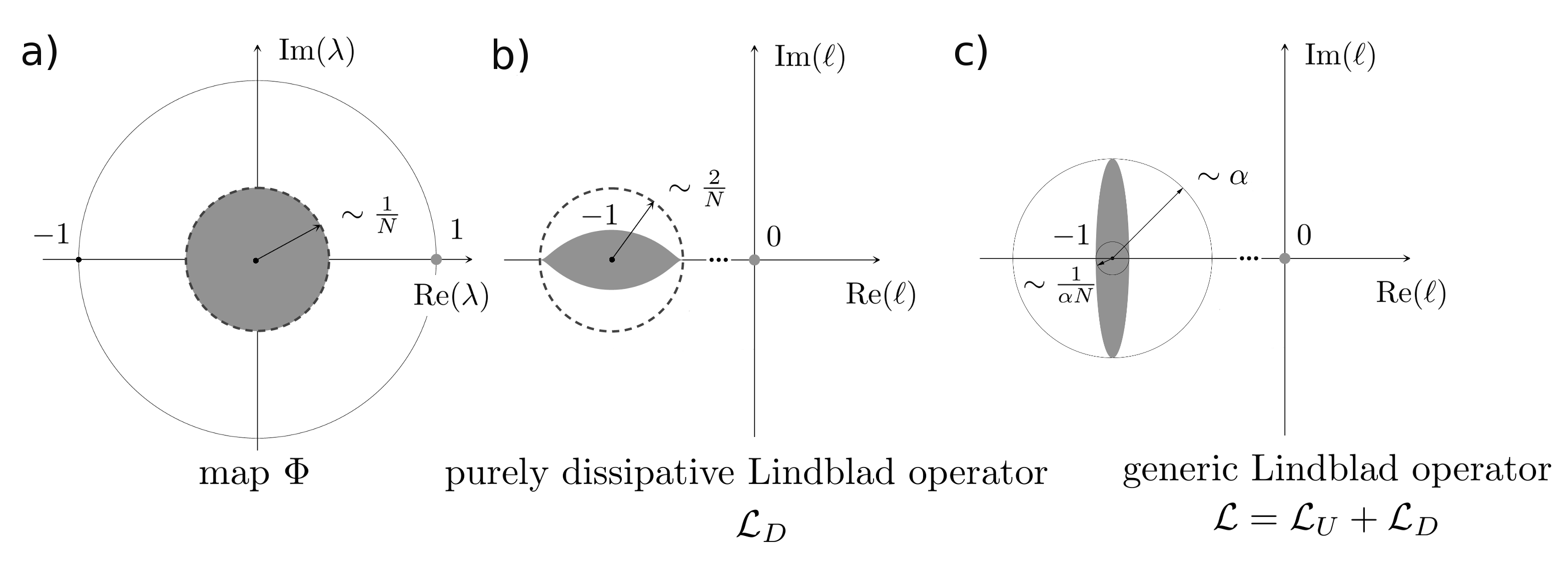
Figure 1: Eigenvalue localization areas (grey) of (a) a random quantum channel, (b) random purely dissipative Lindblad operator, Eq. (3), and (c) random generic Lindbladian with relative weight of the unitary component $\alpha$, Eq. (8). While for the random channel (a) the distribution approaches a Girko’s disc upon the increase of the number of system levels $N$ BCSZ09 , eigenvalues of the random purely dissiaptive Lindblad operator (b) fill the interior of the universal lemon-like contour, Eq. (7). For the Lindblad operator with the unitary component (c), the spectral boundary approaches an ellipse upon increase of $\alpha$.

Similar ideas found applications in disorder systems, single-particle Mirlin and many-body Serbyn ones. From a different perspective, a deep connection to RMT was observed in the models of 2D quantum gravity QG ; QG2 and gauge theories with the large gauge group $U(N)$ Parisi .

In the case of discrete dynamics described by quantum operations, various ensembles of random channels are known BZ17 , including the ensemble in which maps are generated from the entire convex set of quantum operations according to the flat, Hilbert–Schmidt measure BCSZ09 . Recently, powerful methods of random matrices found interesting applications in quantum information theory CN16 ; AS17 . For instance, techniques based on random operations were used by Hastings to refute the celebrated additivity conjecture concerning the minimal output entropy of quantum channels Ha09 .

In the case of continuous quantum dynamics, a class of random Lindblad equations with decay rates obtained by tracing out a random reservoir, was studied in Refs. Bu05 ; BG09 . RMT was applied to open quantum systems in the context of scattering matrices and non-Hermitian effective Hamiltonians, see open-random for a review.

Our perspective in this paper is entirely different: We introduce an ensemble of random Lindblad operators, which describe generic continuous time evolution of an $N$-level open quantum system, and evaluate universal properties of operator spectra. Namely, we analyze the distribution of eigenvalues of a randomly chosen operator $\mathcal{L}$ and study the scaling of spectral characteristics with $N$.

We start the analysis of random Lindbladians by briefly recalling main results concerning random quantum channels BCSZ09 ; BSCSZ10 . Next we analyze the extreme case of purely dissipative evolution, $H=0$ and $\mathcal{L}=\mathcal{L}_{D}$. In this limit we can applies RMT, capture all essential features of the general scenario, and derive equation for the spectral boundary. Finally we address general case, when both unitary and dissipative components, $\mathcal{L}_{U}$ and $\mathcal{L}_{D}$, of the evolution generator, Eq. (1), are present.

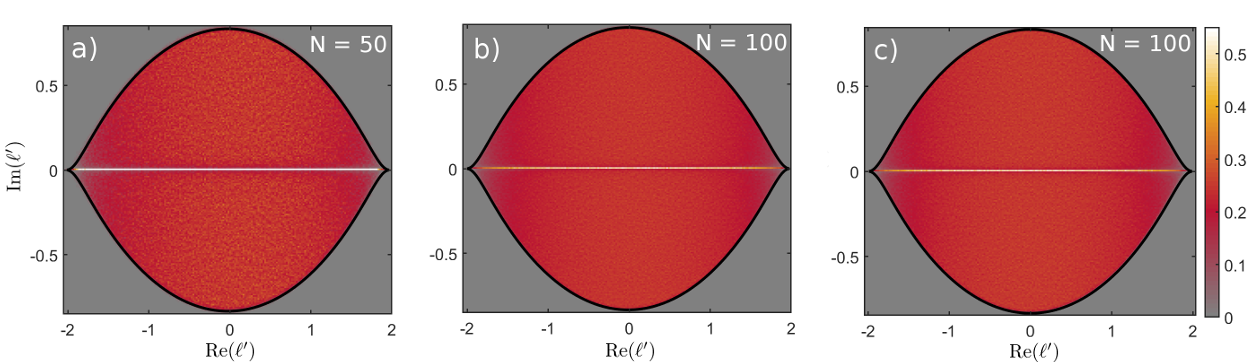
Figure 2: Spectral density $P[\mathrm{Re}(\ell^{\prime}),\mathrm{Im}(\ell^{\prime})]$ of the rescaled eigenvalues, $\ell^{\prime}=N(\ell+1)$, from the spectrum of random purely dissipative Lindblad operators ${\cal L_{D}}$ for $N=50$ and $100$. We use two different sampling procedure for $N=100$, sampling the Kossakowski matrix from the Wishart ensemble (left and middle plots) and an alternative procedure SM (right plot). Note a perfect agreement with the asymptotic boundary of the spectral bulk, Eq. (7) (thick black line), derived with the random matrix model (6). Observe also a concentration of eigenvalues along the real axis, accompanied by depletion nearby – compare to Fig. 3a – which decreases with $N$. Each distribution was sampled with $10^{3}$ realizations.

Random quantum channels. An ensemble of random channels (i.e., completely positive transformations open1 ; open2 ; open3 ) $\Phi:M_{N}(\mathbb{C})\to M_{N}(\mathbb{C})$, can be defined by the flat, Hilbert–Schmidt measure in the space of all quantum operations. It is known that the probability density of the corresponding superoperator $\Phi$ acting on density matrices of order $N$ consists of the leading eigenvalue, $\lambda_{\rm 1}=1$, corresponding to the invariant state, while all remaining eigenvalues fill a disk of radius $R=1/N$ centered at zero; see Fig. 1a. The bulk of the spectrum can be obtained by sampling random matrices $\frac{1}{N}G_{R}$ BCSZ09 with $G_{R}$ being a member of a real Ginibre ensemble Gi65 . Recall that a real Ginibre ensemble of order $N$ is defined by i.i.d. matrix elements with ${\cal N}(0,1/N)$ and asymptotically the distribution of eigenvalues is uniform on the unit disk with a singular component at the real axis FN07 ; girko ; tao .

Thus for a generic superoperator $\Phi$ the size of its spectral gap, $\Delta_{N}=\lambda_{1}-|\lambda_{2}|=1-1/N$, increases with the matrix dimension $N$, so the convergence to equilibrium becomes exponentially fast. For a large $N$ a typical channel becomes close to a one–step contraction, which sends any state into the single invariant state, $\Phi(\rho)=\rho_{\rm inv}=\Phi(\rho_{\rm inv})$. It is known NPPB18 that a generic channel is close to be unital and the correction term, $\Phi({\mathchoice{\rm 1\mskip-4.0mul}{\rm 1\mskip-4.0mul}{\rm 1\mskip-4.5mul}{\rm 1\mskip-5.0mul}})-{\mathchoice{\rm 1\mskip-4.0mul}{\rm 1\mskip-4.0mul}{\rm 1\mskip-4.5mul}{\rm 1\mskip-5.0mul}}$, behaves like a random hermitian matrix of the Gaussian unitary ensemble with asymptotically vanishing norm.

Purely dissipative random Lindblad operators. To generate a random operator $\mathcal{L}_{D}$, we fix an orthonormal Hilbert-Schmidt basis $\{F_{n}\}$ SM and first sample a random Kossakowski matrix $K$. There many ways to do such sampling. However, as we show below, a particular way in which this non-negative order $N^{2}-1$ matrix is sampled is not important: The spectral features of random purely dissipative Lindbaldians are universal.

The most natural way is to sample $K$ from the ensemble of square complex Wishart matrices, distinguished by the fact that it induces the Lebesgue measure in the space of quantum states ZPNC11 . A Wishart matrix pastur has the structure $W=GG^{\dagger}\geq 0$, where $G$ is a complex square Ginibre matrix with independent complex Gaussian entries. Such a choice is physically motivated by the fact that these ensembles of random matrices correspond to non-unitary evolution of quantum dynamical systems under the assumption of classical chaos Haake ; BSCSZ10 .

We use the following normalization condition $\mathrm{Tr}K=N$, that is, $K=NGG^{\dagger}/\mathrm{Tr}GG^{\dagger}$. Note that eigenvalues of $K$, $\gamma_{m}$, $m=1,...,N^{2}-1$, which can be interpreted as decay rates open1 , are distributed according to the universal Marchenko-Pastur law pastur with the mean value $\left<\gamma\right>\sim 1/N$. Diagonalizing the Kossakowski matrix one can reduce the form of $\mathcal{L}_{D}$ as follows:

$$\mathcal{L}_{D}(\rho)=\sum_{m=1}^{N^{2}-1}\gamma_{m}[V_{m}\rho V_{m}^{\dagger}-\frac{1}{2}(V_{m}^{\dagger}V_{m}\rho+\rho V_{m}^{\dagger}V_{m})],$$ (3)

where $V_{m}$ are called ‘noise’ (or ‘jump’) operators to_Campo . Thus $\Phi(\rho)=\sum_{m}\gamma_{m}V_{m}\rho V_{m}^{\dagger}$, defines a Kraus representation of completely positive map. Moreover, $\sum_{m}\gamma_{m}V_{m}^{\dagger}V_{m}=\Phi^{\dagger}({\mathchoice{\rm 1\mskip-4.0mul}{\rm 1\mskip-4.0mul}{\rm 1\mskip-4.5mul}{\rm 1\mskip-5.0mul}})$, where $\Phi^{\dagger}$ is the dual map, ${\rm Tr}[A\cdot\Phi^{\dagger}(B)]={\rm Tr}[\Phi(A)\cdot B]$, and $\mathbb{1}$ is the identity matrix in $M_{N}(\mathbb{C})$. Therefore, Eq. (3) can be rewritten as

$$\mathcal{L}_{D}(\rho)=\Phi(\rho)-\frac{1}{2}\bigl{(}\Phi^{\dagger}(\mathbb{1})\rho+\rho\;\Phi^{\dagger}(\mathbb{1})\bigr{)},$$ (4)

which shows that the purely dissipative Lindblad generator is fully determined by a completely positive map $\Phi$. If, in addition, $\Phi$ is trace-preserving, i.e., it is a quantum channel, we have $\mathcal{L}(\rho)=\Phi(\rho)-\rho$. This is not the case in general, and Hermitian translation matrix, $X=\Phi^{\dagger}({\mathchoice{\rm 1\mskip-4.0mul}{\rm 1\mskip-4.0mul}{\rm 1\mskip-4.5mul}{\rm 1\mskip-5.0mul}})-{\mathchoice{\rm 1\mskip-4.0mul}{\rm 1\mskip-4.0mul}{\rm 1\mskip-4.5mul}{\rm 1\mskip-5.0mul}}$, does not vanish. Making use of this notation, we rewrite the Lindblad operator as ${\cal L}_{D}(\rho)=[\Phi(\rho)-\rho]-\frac{1}{2}(X\rho+\rho X)$.

If $\Phi$ is a quantum channel, the spectrum of ${\cal L}_{D}$ is the spectrum of $\Phi$ shifted by $-1$. Thus the leading eigenvalue, $\lambda_{1}=1$, is translated into $\ell_{1}=0$ and the Girko disk is now centered at $z=-1$. Due to the trace preserving quantum Markovian dynamics, Lindblad generators have always a zero eigenvalue.

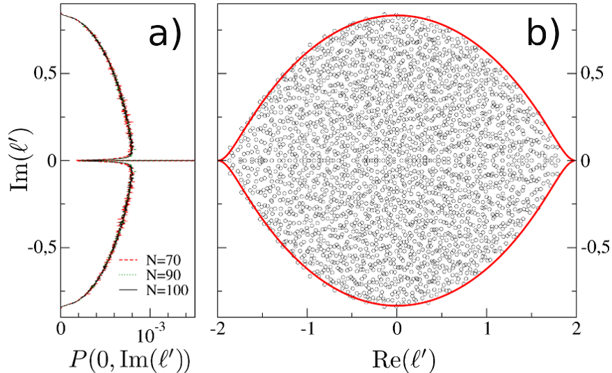
Figure 3: (a) Marginal distribution, $\mathrm{Re}(\ell^{\prime})=0$, of rescaled eigenvalues for three different values of $N$. (b) Rescaled eigenvalues $\ell^{\prime}$ (empty dots) of a single Lindblad operator realization for $N=50$. Red outer contour is the boundary derived from the random matrix model, Eq. (6).

To sample spectra of random Lindbladians, we generate $10^{3}$ realizations for different values of $N$, ranging from $30$ to $100$. In order to reveal the universality of spectra of the operators, it is useful to apply an affine transformation, ${\cal L}_{D}^{\prime}=N({\cal L}_{D}+1)$ SM . Then the bulk of the spectrum of ${\cal L}^{\prime}$ becomes scale invariant and independent of $N$, see Figs. 2 and  3(a).

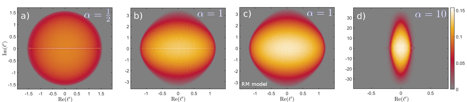
Figure 4: Probability distributions $P[\mathrm{Re}(\ell^{\prime}),\mathrm{Im}(\ell^{\prime})]$ of the rescaled eigenvalues, $\ell^{\prime}=N(\ell+1)$, from the spectrum of random Lindblad operators ${\cal L}$, Eq. (8), for $N=100$ and different values of the unitary component weight $\alpha$. (a,b,d): We present here the results of the sampling of the Kossakowski matrix from the Wishart ensemble, emphasizing that alternative generation procedures SM yield the same results. Panel (c) presents spectral distribution obtained with the random matrix model, Eq.  (10). Each distribution was sampled with $10^{3}$ realizations. Additional normalization of the densities is performed in order to keep maximal values of all distributions equal.

The spectral density inside the ’lemon’ is manifestly non-uniform. Also notable is the eigenvalue concentration along the real axis and the corresponding depletion near by, see Fig 3a. Although ${\cal L}_{D}$ is represented by a complex matrix, it can be made real by a similarity transformation, which explains the effect of concentration FN07 ; tao ; Edelman .

The shape of the sampled eigenvalue distribution $P[\mathrm{Re}(\ell^{\prime}),\mathrm{Im}(\ell^{\prime})]$ is significantly different from the Girko disk and displays a universal lemon–like shape. It is noteworthy that already for $N=50$, a single realization is enough to reproduce the universal shape, see Fig. 3b. From the scale invariance it follows that the spectral gap of ${\cal L}_{D}$ scales as $\Delta_{N}\simeq 1-\frac{2}{N}$. It is clear that the very term $(X\rho+\rho X)$ is responsible for the ‘disk $\to$ lemon’ deformation.

Finally, we performed sampling by using alternative generation procedures SM and for $N\geq 50$ obtained near identical results (differences are within the sampling errors); see Fig. 2 (c). This confirms the universality of the spectral distribution.

Random matrix model — Here we consider a RMT model explaining the observed spectral properties of purely dissipative Lindblad generators. Let us recall that the spectrum of $\mathcal{L}_{D}$ represented in (4) coincides with the spectrum of the following $N^{2}\times N^{2}$ complex matrix $\mathcal{L}_{mn}={\rm Tr}[F_{m}\mathcal{L}_{D}(F_{n})]$. This matrix becomes real if basis matrices $F_{m}$ are hermitian, due to the fact that $\mathcal{L}_{D}$ is hermiticity preserving. Another well known matrix representation of the Lindblad operator reproducing its spectrum reads

$$\widehat{\mathcal{L}}_{D}=\widehat{\Phi}-{\mathchoice{\rm 1\mskip-4.0mul}{\rm 1\mskip-4.0mul}{\rm 1\mskip-4.5mul}{\rm 1\mskip-5.0mul}}\otimes{\mathchoice{\rm 1\mskip-4.0mul}{\rm 1\mskip-4.0mul}{\rm 1\mskip-4.5mul}{\rm 1\mskip-5.0mul}}-\frac{1}{2}(X\otimes{\mathchoice{\rm 1\mskip-4.0mul}{\rm 1\mskip-4.0mul}{\rm 1\mskip-4.5mul}{\rm 1\mskip-5.0mul}}+{\mathchoice{\rm 1\mskip-4.0mul}{\rm 1\mskip-4.0mul}{\rm 1\mskip-4.5mul}{\rm 1\mskip-5.0mul}}\otimes{\overline{X}}),$$ (5)

where $\widehat{\Phi}=\sum_{m=1}^{N^{2}-1}\gamma_{m}V_{m}\otimes\overline{V}_{m}$, and $\overline{V}_{m}$ stands for the complex conjugation. Note that $\widehat{\Phi}$ is neither hermitian nor real, however, the term $X\otimes{\mathchoice{\rm 1\mskip-4.0mul}{\rm 1\mskip-4.0mul}{\rm 1\mskip-4.5mul}{\rm 1\mskip-5.0mul}}+{\mathchoice{\rm 1\mskip-4.0mul}{\rm 1\mskip-4.0mul}{\rm 1\mskip-4.5mul}{\rm 1\mskip-5.0mul}}\otimes{\overline{X}}$ is perfectly hermitian. To understand the spectrum of $\mathcal{L}^{\prime}_{D}$, we use matrix representation (5) approximate its rescaled version with the following random matrix model

$$\widehat{\mathcal{L}}_{D}^{\prime}\approx\,G_{R}-(C\otimes{\mathchoice{\rm 1\mskip-4.0mul}{\rm 1\mskip-4.0mul}{\rm 1\mskip-4.5mul}{\rm 1\mskip-5.0mul}}+{\mathchoice{\rm 1\mskip-4.0mul}{\rm 1\mskip-4.0mul}{\rm 1\mskip-4.5mul}{\rm 1\mskip-5.0mul}}\otimes C).$$ (6)

The matrix $G_{R}$ of size $N^{2}$ is taken from the real Ginibre ensemble. The correction term $C$ approximates $X$ by a symmetric GOE matrix NPPB18 of size $N$.

Matrices are normalized as ${\rm Tr}G_{R}G_{R}^{\dagger}=N^{2}$, so that its spectrum covers uniformly a disk of radius $1$, while ${\rm Tr}C^{2}=N/4$ assures that its density forms the Wigner semicircle of radius $1$. The scaling and parameters of the model follows from the normalization of the Kossakowski matrix SM .

We approach spectral properties of the random matrix model (6) with the quaternionic extension of free probability JanikNowakFRV ; JanikNowak2 ; FeinbergZee ; FeinbergZee2 ; JaroszNowak . Within this framework, we determine the border of the spectrum of ${\cal L}_{D}^{\prime}$ as given by the solution of the following equation involving a complex variable $z$ SM ,

$$\textup{Im}[z+G(z)]=0,$$ (7)

with

$$G(z)=2z-\frac{2z}{3\pi}\left[(4+z^{2})E\left(\frac{4}{z^{2}}\right)+(4-z^{2})K\left(\frac{4}{z^{2}}\right)\right],$$

where $E(k)$ and $K(k)$ are complete elliptic integrals of the first and second kind, respectively. The results of the sampling are in perfect agreement with this border, see Figs. 2-3. Evaluation of the spectral density inside the ’lemon’ is much harder task; it could potentially be performed with diagrammatic techniques JanikNowak2 .

General case of random Lindbladians. Finally, we include unitary component $\mathcal{L}_{U}$ into random Lindblad operator $\mathcal{L}$. For that we need random Hamiltonian $H$, which we sample from the Gaussian Unitary Ensemble (GUE). To compare the spectrum of the general Lindblad operator with a purely dissipative one, we normalize the Hamiltonian, $\rm{Tr}H^{2}=1/N$, and introduce a parameter $\alpha\geq 0$ which weights contribution of the unitary component. The corresponding Lindbladians can be written as [see Eq. (4)]

$$\mathcal{L}(\rho)=-\frac{i\alpha}{\hbar}(H\rho-\rho H)+\Phi(\rho)-\frac{1}{2}\bigl{(}\Phi^{\dagger}(\mathbb{1})\rho+\rho\;\Phi^{\dagger}(\mathbb{1})\bigr{)}.$$ (8)

The sample spectra of the operator ${\cal L}^{\prime}=N({\cal L}+1)$, for different values of $\alpha$, are shown on Fig. 4(a,b,d) (see also in SM ). Similar to the previously considered case of purely dissipative evolution, we find (as expected) a perfect scale invariance of the ${\cal L}^{\prime}$ spectra starting from $N\geq 30$.

The shape of the spectra could be captured with the RMT. First, we transform expression (8) into

$$\widehat{\mathcal{L}}=\widehat{\Phi}-{\mathchoice{\rm 1\mskip-4.0mul}{\rm 1\mskip-4.0mul}{\rm 1\mskip-4.5mul}{\rm 1\mskip-5.0mul}}\otimes{\mathchoice{\rm 1\mskip-4.0mul}{\rm 1\mskip-4.0mul}{\rm 1\mskip-4.5mul}{\rm 1\mskip-5.0mul}}-\left(\frac{1}{2}X+i\alpha H\right)\otimes{\mathchoice{\rm 1\mskip-4.0mul}{\rm 1\mskip-4.0mul}{\rm 1\mskip-4.5mul}{\rm 1\mskip-5.0mul}}+{\mathchoice{\rm 1\mskip-4.0mul}{\rm 1\mskip-4.0mul}{\rm 1\mskip-4.5mul}{\rm 1\mskip-5.0mul}}\otimes\left(\frac{1}{2}{\overline{X}}-i\alpha\overline{H}\right).$$ (9)

The spectrum of $\widehat{\mathcal{L}}$ can be explained by updating the matrix model (6),

$$\widehat{\mathcal{L}}^{\prime}\approx\,G_{R}-(W\otimes{\mathchoice{\rm 1\mskip-4.0mul}{\rm 1\mskip-4.0mul}{\rm 1\mskip-4.5mul}{\rm 1\mskip-5.0mul}}+{\mathchoice{\rm 1\mskip-4.0mul}{\rm 1\mskip-4.0mul}{\rm 1\mskip-4.5mul}{\rm 1\mskip-5.0mul}}\otimes\overline{W}),$$ (10)

where $G_{R}$ of size $N^{2}$ is again taken from the real Ginibre ensemble, while the extended correction term $W=C+i\alpha H^{\prime}$ contains now a random GOE matrix $C$ and an anti-hermitian term proportional to a GUE matrix $H^{\prime}$ of order $N$ normalized as ${\rm Tr}H^{\prime 2}=N$. Spectral density of the RMT model for $\alpha=1$ is shown in Fig. 4(c). It reproduced the density of the corresponding Linbladian ensemble (except of eigenvalue concentration at the real axis FN07 ; tao ; Edelman ).

The eigenvalues of $W$ uniformly cover an ellipse with semi-axes $\frac{1}{\sqrt{1+4\alpha^{2}}}$ and $\frac{4\alpha^{2}}{\sqrt{1+4\alpha^{2}}}$. Spectral density of $\widehat{\mathcal{L}}^{\prime}$ is therefore a (classical) convolution of two uniform densities supported on these ellipses followed by free convolution with the Girko disk of unit radius; see sketch on Fig. 1(c). Contrary to the case of purely dissipative Lindbladians, it is hardly possible to determine analytically spectral boundary of general Lindbladian ensembles. However, when $\alpha=\frac{1}{2}$, it immediately follows (since a convolution of two discs is a disc) that the spectral boundary is a circle. This is in full agreement with the results of the sampling; see Fig. 4(a).

Conclusions. Our results constitute a step toward a spectral theory of dissipative Quantum Chaos brown ; BSCSZ10 . Universal spectral features of different ensembles of unitary evolution generators – that are Hamiltonians – are the main pillar of the existing Quantum Chaos (QC) theory Haake . A notion of an ensemble of random operators of quantum Markovian evolution is therefore necessary to extend QC into the area of open quantum systems. The two next steps would be (i) establishing of links between the idea of ’typical Lindbladian’ and physical models displaying chaotic dynamics (open systems that exhibit many-body localization at the Hamiltonian limit are prospective candidates mbl1 ; mbl2 ), and (ii) evaluation of spectral properties of steady states of random Lindbladians.

Finally, it should also be stressed that our approach works equally well in the classical case, where continuous dynamics in the space of probability distributions is determined by Kolmogorov generators else .

Note added: One of the authors (W.T.) attended a talk by Tankut Can given at the conference in Yad Hashmona (Israel) in October 2018, in which a parallel project on random Lindblad operators was presented. Since the first version of this work was posted in the arXiv in November 2018, three other papers on the related subjects appeared C19 ; COOG19 ; SRP19 .

I Supplemental Material

I.1 Sampling of random Lindblad operators

Due to the unitary equivalence, the particular choice of a Hilbert-Schmidt basis to construct a Kossakowski matrix is not important. As $\{F_{n}\}$ ($n=1,\ldots,N^{2}-1$) we take the full set of infinitesimal generators of $SU(N)$ (see, e.g., Alicki ). Namely, let $|1\rangle,\ldots|N\rangle$ be an orthonormal basis in $N$-dimensional Hilbert space. The generators of $SU(N)$ are defined as the following $N^{2}-1$ Hermitian matrices:

• $N(N-1)/2$ symmetric,

  $$S_{jk}=\frac{1}{\sqrt{2}}\Big{(}|j\rangle\langle k|+|k\rangle\langle j|\Big{)}\ ,\ \ 1\leq j<k\leq N$$

• $N(N-1)/2$ antisymmetric,

  $$J_{jk}=-\frac{i}{\sqrt{2}}\Big{(}|j\rangle\langle k|-|k\rangle\langle j|\Big{)}\ ,\ \ 1\leq j<k\leq N$$

• and $N-1$ diagonal

  $$D_{l}=\frac{1}{\sqrt{l(l+1)}}\left(\sum_{k=1}^{l}|k\rangle\langle k|-l|l+1\rangle\langle l+1|\right)\ ,$$

  for $1\leq l\leq N-1$.

For $N=2$ this recipe yields Pauli matrices while for $N=3$ it results in the standard eight Gell-Mann matrices.

A brute-force sampling by using Eq. (1) becomes extremely slow and ineffective already with $N=30$. A single-core implementation of such sampling cannot produce a single realization for $N=100$ on the time scale of several days. To overcome this bottleneck, we parallelize the sampling procedure and realize it on a large computational cluster. The detailed information will be presented in a separate paper [S1]; here we only briefly outline two key steps.

First, in order to multiple matrices in Eq. (1), we avoided standard built-on matrix-matrix multiplications because the matrices to multiple a Kossakowski matrix with are very sparse. So this operation has been encoded explicitly, in the element-wise manner.

Second, calculation of the summands on the rhs of Eq. (1), together with corresponding multiplications, was performed in parallel, on several cores simultaneously, and then the results were summed up.

Sampling simulations were performed on the Lobachevsky supercomputer (Nizhny Novgorod) and the MPIPKS cluster (Dresden).

I.2 Sampling of the Kossakowski matrix

Under normalization condition $\mathrm{Tr}K=N$, sampling of the positive semi-definite matrix $K$ reduces to the sampling of a random density matrix [SM2]. We considered different sampling procedures listed in Table I of Ref. [SM2],

$$K=N\frac{SS^{\dagger}}{\mathrm{Tr}SS^{\dagger}},~{}~{}~{}~{}S[k,s]:=[p_{1}U_{1}+p_{2}U_{2}+...+p_{k}U_{k}]G_{1}G_{2}...G_{s},$$ (S1)

where $p=\{p_{1},...,p_{k}\}$ is a random probability vector, $U_{1},...,U_{k}$ is a set of $k$ independent random unitary matrices distributed according to the Haar measure on $U(N)$ and $G_{1},...,G_{s}$ is a set of independent $N\times N$ random matrices sampled from the complex Ginibre ensemble. In the case $k=s=1$ it reduces to the sampling described in the main text (and which leads to the Marchenko-Pastur distributions of the $K$’s eigenvalues). We also used combinations $\{k=1,s=2,3,7\}$ [leading to the Fuss–Catalan distributions $\pi(s)$] and $\{k=2,s=0,1\}$ [leading to the arcsine and Bures ensembles [S2], respectively]. Finally, we used a more exotic sampling procedure,

$$K=N\frac{UD}{\mathrm{Tr}UD},$$ (S2)

with $U$ being a random unitary matrix sampled according to the Haar measure on $U(N)$ and $D$ being a diagonal core of the singular-value decomposition (SVD), $G=VDW$, of a random matrix $G$ sampled from the complex Ginibre ensemble (the results of the sampling are shown in Fig. 2 (middle panel) of the main text). In all cases we did not observe noticeable difference in the sampled spectral densities (more formally, the differences were within sampling errors).

To summarize, it is not important, from the spectral point of view, how the manifold of all random Lindlad generators, acting in the $N$-dimensional Hilbert-Schmidt space, is sampled – provided that the sampling is not ’pathological’ (f.e., $K$ is not restricted to a low-rank manifold) and normalization $\mathrm{Tr}K=N$ is kept.

In this section we also present distributions sampled for random Lindblad operators, with unitary component $\mathcal{L}_{U}$ included, for $\alpha=10$ and $\alpha=100$; see Fig. 1.

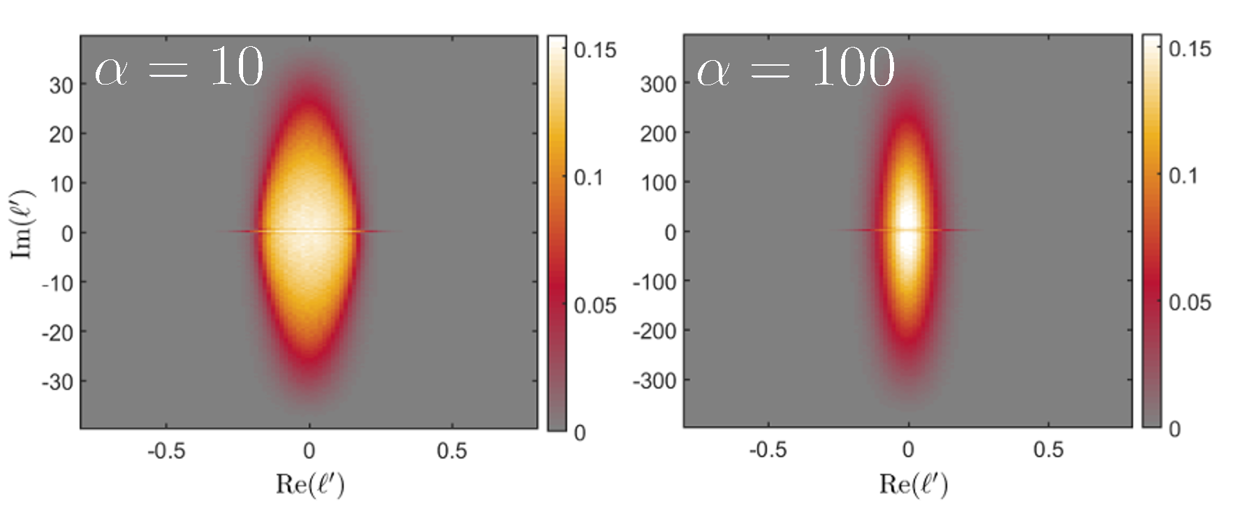
Figure S1: Probability distributions $P(\mathrm{Re}(\ell^{\prime}),\mathrm{Im}(\ell^{\prime}))$ of the rescaled eigenvalues, $\ell^{\prime}=N(\ell+1)$, from the bulk of the spectrum of random Lindblad operators ${\cal L}$, Eq (8) in the main text, for $N=100$ and two different values of the unitary component weight $\alpha$. We present here the results of the sampling of the Kossakowski matrix from the Wishart ensemble emphasizing that alternative generation procedures yield the same results. Each distribution was sampled with $10^{3}$ realizations. Additional normalization of the densities is performed in order to keep maximal values of all distributions equal.

I.3 Justification of the random matrix model

Since the Kossakowski matrix is positive definite, it can be decomposed as $K=Z^{\dagger}Z$. If the normalization condition $\textup{Tr}K=N$ is relaxed to $\left<\textup{Tr}K\right>=N$, then elements of $X$ are i.i.d. Gaussian random variables with the variance

$$\left<Z_{ab}Z^{\dagger}_{cd}\right>=\frac{N}{(N^{2}-1)^{2}}\delta_{ad}\delta_{bc}.$$ (S3)

We define a set of $N\times N$ matrices $Y_{a}=\sum_{m=1}^{N^{2}-1}Z_{am}F_{m}$ for $a=1,\ldots,N^{2}-1$. Note that due to independence of rows of $Z$, matrices $Y_{a}$ are independent. Moreover, probability distribution for elements of $Z$ is invariant under unitary transformations $Z\to ZU$, thus the statistical distribution of elements of $Y_{a}$ is the same, irrespective of the choice of basis matrices $F_{m}$. This convinces us that the entries of $Y_{a}$ are almost independent (the only constraint is $\textup{Tr}Y_{a}=0$), thus in the large $N$ limit eigenvalues of $Y_{a}$ cover uniformly the disk of radius $r$, where

$$r^{2}=\left<\frac{1}{N}\textup{Tr}Y_{a}Y^{\dagger}_{a}\right>=\frac{1}{N^{2}-1}.$$ (S4)

Here we used the orthogonality of basis $\textup{Tr}F_{m}F^{\dagger}_{n}=\delta_{mn}$ and (S3).

Matrices $Y_{a}$ allow us to rewrite the Lindblad operator as

$$\hat{{\cal L}}=\hat{\Phi}-{\mathchoice{\rm 1\mskip-4.0mul}{\rm 1\mskip-4.0mul}{\rm 1\mskip-4.5mul}{\rm 1\mskip-5.0mul}}\otimes{\mathchoice{\rm 1\mskip-4.0mul}{\rm 1\mskip-4.0mul}{\rm 1\mskip-4.5mul}{\rm 1\mskip-5.0mul}}-(X\otimes{\mathchoice{\rm 1\mskip-4.0mul}{\rm 1\mskip-4.0mul}{\rm 1\mskip-4.5mul}{\rm 1\mskip-5.0mul}}+{\mathchoice{\rm 1\mskip-4.0mul}{\rm 1\mskip-4.0mul}{\rm 1\mskip-4.5mul}{\rm 1\mskip-5.0mul}}\otimes\overline{X}),$$ (S5)

with

$$\hat{\Phi}=\sum_{a=1}^{N^{2}-1}Y_{a}\otimes\overline{Y}_{a},$$ (S6)

$$2X=-{\mathchoice{\rm 1\mskip-4.0mul}{\rm 1\mskip-4.0mul}{\rm 1\mskip-4.5mul}{\rm 1\mskip-5.0mul}}+\sum_{a=1}^{N^{2}-1}Y_{a}^{\dagger}Y_{a}.$$ (S7)

All $N^{2}$ eigenvalues of $Y_{a}\otimes\overline{Y}_{a}$ are in the form of $\lambda_{i}\overline{\lambda}_{j}$ for $i,j=1,\ldots,N$, where $\lambda_{i,j}$ are eigenvalues of $Y_{a}$, thus their density is supported on a disk of radius $(N^{2}-1)^{-1}$. $\hat{\Phi}$ is a sum of $N^{2}-1$ independent matrices $Y_{a}\otimes\overline{Y}_{a}$, thus, according to the central limit theorem for non-hermitian matrices, its spectral density is uniform on the disk of radius $(N^{2}-1)^{-1/2}$. As a consequence, in the large $N$ limit, $\hat{\Phi}$ can be modelled as a Ginibre matrix with the spectral radius $1/N$.

It is also clear that the matrix $W_{a}=\frac{1}{2}\left(Y^{\dagger}_{a}Y_{a}-\frac{{\mathchoice{\rm 1\mskip-4.0mul}{\rm 1\mskip-4.0mul}{\rm 1\mskip-4.5mul}{\rm 1\mskip-5.0mul}}}{N^{2}-1}\right)$ is a shifted and rescaled Wishart matrix, and its spectral density has zero mean and variance $\sigma^{2}=\frac{1}{4(N^{2}-1)^{2}}$. Since $X$ is a sum of $N^{2}-1$ independent such matrices, according to the central limit theorem for hermitian matrices, its spectral density is the Wigner semicircle supported on $[-1/N,1/N]$ with density

$$\rho_{X}(x)=\frac{2N^{2}}{\pi}\sqrt{\frac{1}{N^{2}}-x^{2}}.$$ (S8)

The above reasoning correctly predicts the $1/N$ scaling and unit shift $\hat{{\cal L}}=-{\mathchoice{\rm 1\mskip-4.0mul}{\rm 1\mskip-4.0mul}{\rm 1\mskip-4.5mul}{\rm 1\mskip-5.0mul}}+\frac{1}{N}\hat{{\cal L}}^{\prime}$ and justifies the following approximation of $\hat{{\cal L}}^{\prime}$

$$\hat{{\cal L}}^{\prime}\approx G_{R}-(C\otimes{\mathchoice{\rm 1\mskip-4.0mul}{\rm 1\mskip-4.0mul}{\rm 1\mskip-4.5mul}{\rm 1\mskip-5.0mul}}+{\mathchoice{\rm 1\mskip-4.0mul}{\rm 1\mskip-4.0mul}{\rm 1\mskip-4.5mul}{\rm 1\mskip-5.0mul}}\otimes\overline{C}).$$ (S9)

While the matrix representation of Lindblad operator (S5) is not real, $\overline{\hat{{\cal L}}}\neq\hat{{\cal L}}$, it is related to its complex conjugate via a similarity transformation $\overline{\hat{{\cal L}}}=P\hat{{\cal L}}P$ by a symmetric permutation matrix $P$ with a property that for any two matrices $A,B$ of size $N^{2}$

$$P(A\otimes B)P=B\otimes A$$ (S10)

holds. Therefore one can take $G_{R}$ as a real Ginibre matrix and $C$ as a symmetric GOE matrix so that $\overline{C}=C$.

To take into account Hamiltonian part of the dynamics our random matrix model (S9) can be generalized to include also a purely antihermitian part,

$$L=G_{R}-{\mathchoice{\rm 1\mskip-4.0mul}{\rm 1\mskip-4.0mul}{\rm 1\mskip-4.5mul}{\rm 1\mskip-5.0mul}}\otimes{\mathchoice{\rm 1\mskip-4.0mul}{\rm 1\mskip-4.0mul}{\rm 1\mskip-4.5mul}{\rm 1\mskip-5.0mul}}-\alpha(C\otimes{\mathchoice{\rm 1\mskip-4.0mul}{\rm 1\mskip-4.0mul}{\rm 1\mskip-4.5mul}{\rm 1\mskip-5.0mul}}+{\mathchoice{\rm 1\mskip-4.0mul}{\rm 1\mskip-4.0mul}{\rm 1\mskip-4.5mul}{\rm 1\mskip-5.0mul}}\otimes{\overline{C}})+i\beta(H\otimes{\mathchoice{\rm 1\mskip-4.0mul}{\rm 1\mskip-4.0mul}{\rm 1\mskip-4.5mul}{\rm 1\mskip-5.0mul}}-{\mathchoice{\rm 1\mskip-4.0mul}{\rm 1\mskip-4.0mul}{\rm 1\mskip-4.5mul}{\rm 1\mskip-5.0mul}}\otimes{\overline{H}}),$$ (S11)

which will be analyzed in a separate paper. Here $H$ denotes a Hermitian random matrix of order $N$ from the GUE ensemble representing a generic Hamiltonian.

I.4 A spectrum of the matrix model for the Lindblad operator

I.4.1 Quaternionic free probability

Here we briefly review the quaternionic extension of free probability to nonhermitian random matrices, developed in [S3-S7] (see also [S8] for a recent rigorous treatment), focusing mostly on the aspects relevant for this study. For a pedagogical introduction and more explicit calculations we refer to [S9]

The main object of interest is the spectral density $\rho(z,\bar{z})=\left<\frac{1}{N}\sum_{i=1}^{N}\delta^{(2)}(z-\lambda_{i})\right>$ on the complex plane. Here $\delta^{(2)}(z)=\delta(\textup{Re}z)\delta(\textup{Im}z)$. The density is obtained via the Poisson law $\rho(z,\bar{z})=\lim_{|w|\to 0}\frac{1}{\pi}\partial_{z\bar{z}}\Phi(z,\bar{z},w,\bar{w})$, where $\Phi$ is the (regularized) electrostatic potential in two dimensions [S10],

$$\Phi(z,\bar{z},w,\bar{w})=\left<\frac{1}{N}\ln\det\left[(z-X)(\bar{z}-X^{\dagger})+|w|^{2}\right]\right>.$$ (S12)

To facilitate the calculations in large $N$ limit, one considers the generalized Green’s function, which is a $2\times 2$ matrix

$${\cal G}(Q)=\left<\frac{1}{N}\textup{bTr}\left(Q\otimes\mathbb{1}-{\cal X}\right)^{-1}\right>=\left(\begin{array}[]{cc}{\cal G}_{11}&{\cal G}_{12}\\ {\cal G}_{21}&{\cal G}_{22}\end{array}\right),$$ (S13)

with

$$Q=\left(\begin{array}[]{cc}z&i\bar{w}\\ iw&\bar{z}\end{array}\right),\quad{\cal X}=\left(\begin{array}[]{cc}X&0\\ 0&X^{\dagger}\end{array}\right),$$ (S18)

where we also introduced a block trace (partial trace) operation

$$\textup{bTr}\left(\begin{array}[]{cc}A&B\\ C&D\end{array}\right)=\left(\begin{array}[]{cc}\textup{Tr}A&\textup{Tr}B\\ \textup{Tr}C&\textup{Tr}D\end{array}\right).$$ (S23)

Note that $Q$ is a matrix representation of a quaternion, thus we refer to this approach as quaternionic free probability. The upper-left element of ${\cal G}$ yields spectral density via $\rho(z,\bar{z})=\lim_{|w|\to 0}\frac{1}{\pi}\partial_{\bar{z}}{\cal G}_{11}$, while the product of off-diagonal elements yields the correlation function capturing non-orthogonality of eigenvectors [S11-S13]. An important fact for this paper is that the boundary of the spectrum can be determined from the condition ${\cal G}_{12}{\cal G}_{21}=0$.

Knowing the Green’s function, one defines also the Blue’s function as its functional inverse

$${\cal B}({\cal G}(Q))=Q,\quad{\cal G}({\cal B}(Q))=Q.$$ (S24)

Then, the quaternionic $R$-transform is defined as ${\cal R}(Q)={\cal B}(Q)-Q^{-1}$, where the inverse is understood in the sense of $2\times 2$ matrix inversion. When two nonhermitian matrices $A$ and $B$ are free, then the $R$-transform of their sum is a sum of corresponding $R$-transforms

$${\cal R}_{A+B}(Q)={\cal R}_{A}(Q)+{\cal R}_{B}(Q).$$ (S25)

In that sense, it generalizes the logarithm of the Fourier transform from classical probability to the noncommutative case.

I.4.2 Nonhermitian Pastur equation

We now consider a problem of finding a spectrum of the matrix $A+B$, where $A$ is a Ginibre matrix and $B$ can be arbitrary. Starting with (S25), we add $Q^{-1}$ to both sides, obtaining

$${\cal B}_{A+B}(Q)={\cal R}_{A}(Q)+{\cal B}_{B}(Q).$$ (S26)

Then we make a substitution $Q\to{\cal G}_{A+B}(Q)$ and use the relation between Green’s and Blue’s function (S24), obtaining

$$Q-{\cal R}_{A}({\cal G}_{A+B}(Q))={\cal B}_{B}({\cal G}_{A+B}(Q)).$$ (S27)

In the next step we evaluate the Green’s function of $B$ at both sides of equation and use (S24) to get

$${\cal G}_{B}(Q-{\cal R}_{A}({\cal G}_{A+B}(Q)))={\cal G}_{A+B}(Q),$$ (S28)

which is the nonhermitian Pastur equation. In our case $A$ is Ginibre, the $R$-transform of which reads

$${\cal R}_{A}({\cal G}_{A+B})=\left(\begin{array}[]{cc}0&{\cal G}_{12}\\ {\cal G}_{21}&0\end{array}\right),$$ (S31)

thus (S28) simplifies to

$${\cal G}_{B}\left[\left(\begin{array}[]{cc}z&-{\cal G}_{12}\\ -{\cal G}_{21}&\bar{z}\end{array}\right)\right]=\left(\begin{array}[]{cc}{\cal G}_{11}&{\cal G}_{12}\\ {\cal G}_{21}&{\cal G}_{22}\end{array}\right),$$ (S36)

where we suppressed index ‘$A+B$’ when writing components of ${\cal G}_{A+B}$. We also used the fact that all important quantities are calculated in the $|w|\to 0$ limit and took this limit at the level of this algebraic equation.

I.4.3 Embedding of hermitian matrices

Equation (S36) is true for general (even not necessarily random) matrix $B$, but the quaternionic Green’s function can be easily obtained for Hermitian matrices. In such a case it reads [S6]

$${\cal G}(Q)=\gamma(q,\bar{q})\mathbb{1}_{2}-\gamma^{\prime}(q,\bar{q})Q^{\dagger},$$ (S37)

with

$$\gamma(q,\bar{q})=\frac{qG(q)-\bar{q}G(\bar{q})}{q-\bar{q}},$$ (S38)

$$\gamma^{\prime}(q,\bar{q})=\frac{G(q)-G(\bar{q})}{q-\bar{q}},$$ (S39)

where $q,\bar{q}$ are the eigenvalues of the $2\times 2$ quaternion matrix (S18) and $G(z)$ is the Stieltjes transform of the spectral density of $B$

$$G(z)=\int_{-\infty}^{+\infty}\frac{\rho_{B}(x)dx}{z-x}.$$ (S40)

I.4.4 Border of the spectrum

We are now ready to solve equation (S36). Focusing on the component ${\cal G}_{12}$ of this matrix equation and using $\bar{{\cal G}}_{21}=-{\cal G}_{12}$, which follows from the definition of the quaternion (S18), we obtain

$$-\frac{G(q)-G(\bar{q})}{q-\bar{q}}{\cal G}_{12}={\cal G}_{12}.$$ (S41)

Now $q,\bar{q}$ are the eigenvalues of the matrix

$$\left(\begin{array}[]{cc}z&-{\cal G}_{12}\\ -{\cal G}_{21}&\bar{z}\end{array}\right).$$ (S44)

There is one trivial solution, ${\cal G}_{12}=0$, which is valid outside the spectrum. Inside the spectrum one has ${\cal G}_{12}\neq 0$, but these two solutions match at the border of the spectrum, providing the equation for it. Note that for ${\cal G}_{12}=0={\cal G}_{21}$ eigenvalues of (S44) are just $z,\bar{z}$, thus we immediately obtain the equation for the borderline from (S41):

$$G(z)-G(\bar{z})=\bar{z}-z.$$ (S45)

To solve a more general problem, namely spectrum of $A+\alpha B$ we use the fact that the Stieltjes transform of the rescaled matrix $\alpha B$ is given by the Stieltjes transform of the original matrix $B$ via $G_{\alpha B}(z)=\frac{1}{\alpha}G_{B}(\frac{z}{\alpha})$, we get the final form:

$$\textup{Im}\left[\alpha z+G\left(\frac{z}{\alpha}\right)\right]=0.$$ (S46)

In our model we set $\alpha=1$. To find the spectrum of the Kolmogorov generator, we take $B$ with Gaussian spectrum and then

$$G_{\textup{class}}(z)=\frac{1}{\sqrt{2\pi}}\int_{-\infty}^{\infty}\frac{e^{-x^{2}/2}}{z-x}dx=\sqrt{\frac{\pi}{2}}e^{-z^{2}/2}\left(\textup{Erfi}\left(\frac{z}{\sqrt{2}}\right)-i\textup{sgn}(\textup{Im}z)\right)$$ (S47)

I.4.5 Stieltjes transform of $1\otimes C+C\otimes 1$

In order to solve (S46), we aim to find the Stieltjes transform of $B=1\otimes C+C\otimes 1$. Note that each eigenvalue of $B$ is of the form $\lambda=\mu_{a}+\mu_{b}$, where $\mu_{a,b}$ are the eigenvalues of $C$. Taking $C$ as GOE, the spectral density of which is the Wigner semicircle, $\rho_{C}(x)=\frac{2}{\pi}\sqrt{1-x^{2}}$, the spectrum of $B$ is therefore the (classical) convolution of two Wigner semicircles. This can be calculated using standard tools from probability. The Fourier transform of the Wigner semicircle is $\tilde{\rho}_{C}(k)=\frac{2}{k}J_{1}(k)$, where $J_{1}$ is the Bessel function of the first kind. Therefore the Fourier transform of $B$ reads $\tilde{\rho}_{B}(k)=\frac{4}{k^{2}}J_{1}^{2}(k)$. To calculate the Stieltjes transform of $B$ we use the following representation $(z-x)^{-1}=\mp i\int_{0}^{\infty}e^{\pm ip(z-x)}dx$, which allows us to calculate the Stieltjes transform directly from the Fourier transform via $G(z)=\mp i\int_{0}^{\infty}e^{\pm ipz}\tilde{\rho}_{B}(\mp p)dp$, where we take the upper signs for $\textup{Im}z>0$ and lower for $\textup{Im}z<0$. The final result reads

$$G(z)=2z-\frac{2z}{3\pi}\left[(4+z^{2})E\left(\frac{4}{z^{2}}\right)+(4-z^{2})K\left(\frac{4}{z^{2}}\right)\right],$$ (S48)

where $K(z)$ and $E(z)$ are the complete elliptic integrals of the first and second kind, respectively. Substitution into (S46) yields an implicit equation which is then solved numerically, see Fig. 2 for comparison with the numerical simulations.

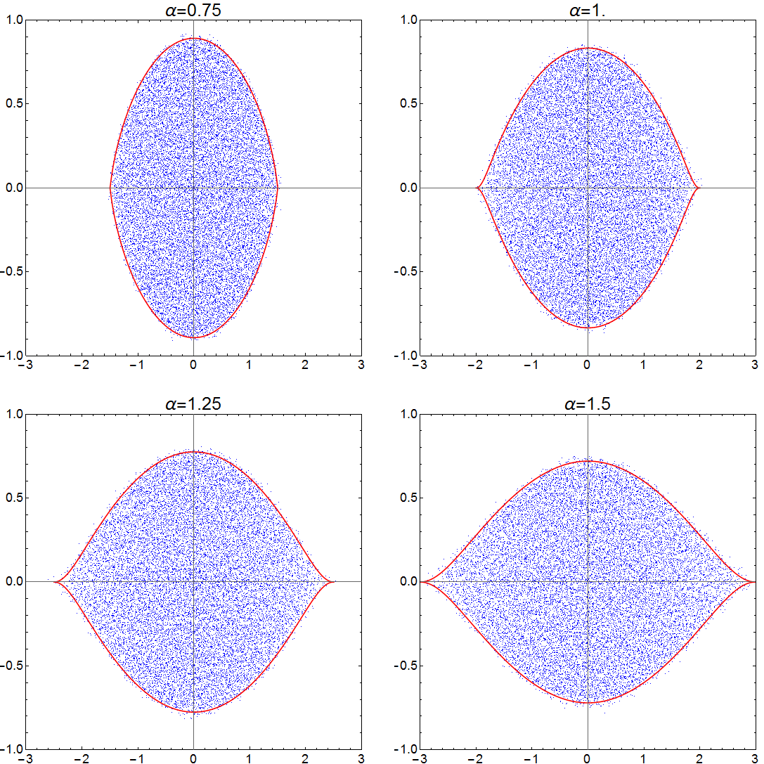
Figure S2: Spectra of the random matrix model $G_{R}+\alpha(C\otimes{\mathchoice{\rm 1\mskip-4.0mul}{\rm 1\mskip-4.0mul}{\rm 1\mskip-4.5mul}{\rm 1\mskip-5.0mul}}+{\mathchoice{\rm 1\mskip-4.0mul}{\rm 1\mskip-4.0mul}{\rm 1\mskip-4.5mul}{\rm 1\mskip-5.0mul}}\otimes C)$ for $\alpha=0.75,1.0,1.25,1.5$. The borderline of the asymptotic spectrum was calculated numerically from (S46). Points are obtained from the numerical diagonalization of 20 independent matrices of size $N^{2}=900$.

Interestingly, the technique used to derive the presented results opens a new application area for the theory of free probability [S14]. Our usage of the theory is based on a two-step procedure: the classical convolution of two Hermitian ensembles is followed by a free convolution with the Ginibre ensemble.

References

[S1] I. Meyerov, A. Liniov, E. Kozinov, V. Volokitin, M. Ivanchenko, and S. Denisov, Unfolding quantum master equation into a system of linear equations: computationally effective expansion over the basis of $SU(N)$ generators, arXiv:1812.11626.

[S2] K. Życzkowski, K. A. Penson, I. Nechita, and B. Collins, Generating random density matrices, J. Math. Phys. E 52, 062201 (2011).

[S3] R. A. Janik, M. A. Nowak, G. Papp, J. Wambach and I. Zahed, Non-Hermitian random matrix models: Free random variable approach, Phys. Rev. E 55 (4), 4100 (1997).

[S4] R. A. Janik, M. A. Nowak, G. Papp, I. Zahed, Non-hermitian random matrix models, Nucl. Phys. B 501 (3), 603 (1997).

[S5] J. Feinberg, A. Zee, Non-Gaussian non-Hermitian random matrix theory: phase transition and addition formalism, Nucl. Phys.B 501 (3), 643 (1997).

[S6] J. Feinberg, A. Zee, Non-hermitian random matrix theory: Method of hermitian reduction, Nucl. Phys. B 504 (3), 579 (1997).

[S7] A. Jarosz, M. A. Nowak, Random Hermitian versus random non-Hermitian operators—unexpected links, J. Phys. A: Math. Gen. 39 (32), 10107 (2006).

[S8] S. T. Belinschi, P. Śniady, R. Speicher, Eigenvalues of non-hermitian random matrices and Brown measure of non-normal operators: hermitian reduction and linearization method, Linear Algebra Appl. 537, 48 (2018).

[S9] M.A. Nowak and W. Tarnowski, Spectra of large time-lagged correlation matrices from random matrix theory, J. Stat. Mech.: Th. Exp. 2017, 063405 (2017).

[S10] H.J. Sommers, A. Crisanti, H. Sompolinsky and Y. Stein, Spectrum of large random asymmetric matrices, Phys. Rev. Lett. 60, 1895 (1988).

[S11] J. T. Chalker and B. Mehlig, Eigenvector statistics in non-Hermitian random matrix ensembles, Phys. Rev. Lett. 81, 3367 (1998).

[S12] B. Mehlig and J. T. Chalker, Statistical properties of eigenvectors in non-Hermitian Gaussian random matrix ensembles, J. Math. Phys. 41, 3233 (2000).

[S13] R.A. Janik, W. Nörenberg, M.A. Nowak, G. Papp, and I. Zahed, Correlations of eigenvectors for non-Hermitian random-matrix models, Phys. Rev. E 60, 2699 (1999).

[S14] J. A. Mingo and R. Speicher, Free probability and random matrices, (Springer Science, New York, 2017).