Distribution of high-dimensional orbital angular momentum entanglement at telecom wavelength over 1km vortex fiber

Abstract

High-dimensional entanglement has demonstrated potential for increasing channel capacity and resistance to noise in quantum information processing. However, its distribution is a challenging task, imposing a severe restriction on its application. Here we report the first distribution of three-dimensional orbital angular momentum (OAM) entanglement via a 1-km-long optical fibre. Using an actively-stabilising phase precompensation technique, we successfully transport one photon of a three-dimensional OAM entangled photon pair through the fibre. The distributed OAM entangled state still shows a fidelity up to 71% with respect to the three-dimensional maximal-entangled-state (MES). In addition, we certify that the high-dimensional quantum entanglement survives the transportation by violating a generalised Bell inequality, obtaining a violation of $\sim 3$ standard deviations with $I_{3}=2.12\pm 0.04$. The method we developed can be extended to higher OAM dimension and larger distances in principle. Our results make a significant step towards future OAM-based high-dimensional long distance quantum communication.

I INTRODUCTION

Increasing the channel capacity and tolerance to noise in quantum communications are strong practical motivations for encoding quantum information in multilevel systems, qudits as opposed to qubits Fujiwara et al. (2003); Bechmann-Pasquinucci and Tittel (2000); Gisin et al. (2002); Aolita and Walborn (2007); Ali-Khan et al. (2007); D’Ambrosio et al. (2012); Nunn et al. (2013); Mower et al. (2013); Graham et al. (2015); Langford et al. (2004). From a foundational perspective, entanglement in higher dimensions exhibits more complex structures Dada et al. (2011); Romero et al. (2012); Giovannini et al. (2013); Krenn et al. (2014); Malik et al. (2016), and stronger nonclassical correlations Collins et al. (2002). Despite these benefits, the distribution of high-dimensional entanglement is relatively new and remains challenging. We improve on previous works Löffler et al. (2011); Kang et al. (2012) by (1) distributing three-dimensional—rather than two-dimensional—entanglement, and (2) increasing the length of the fibre by three orders of magnitude—achieving the first OAM entanglement distribution via fibre in the kilometer regime.

Inside the laboratory three-level qutrit quantum teleportation has been achieved Luo et al. (2019); Hu et al. (2019). To bring the benefit of qudits into practice, long-distance shared entanglement is required. To this end, a 10-dimensional entangled state has been transmitted over a 24-km long fibre using frequency modes Kues et al. (2017); a 4-dimensional entangled state has been transmitted over 100-km long fibre using time-bins Ikuta and Takesue (2018). Hybrid polarisation-time bin entanglement has also been distributed across a 1.2-km free-space intracity link Steinlechner et al. (2017). Distributing entanglement using spatial degrees of freedom, like path and transverse spatial modes, has also been achieved albeit on very modest scales: 4-dimensional path entanglement over a 30-cm long multi-core fibre Lee et al. (2017), and 2-dimensional transverse spatial mode entanglement over a 30-cm hollow photonic crystal fibre Löffler et al. (2011) and 40-cm step-index fibre Kang et al. (2012). Our work improves on these last two results by showing qutrit entanglement transport through fibre in the kilometer regime.

Spontaneous parametric down-conversion (SPDC) naturally conserves both energy and momentum. As a consequence, entanglement in temporal and spatial degrees of freedom (DOF) comes naturally. These two DOFs are both suitable to be used as qudits. We focus on the transverse spatial modes associated with photonic OAM. An OAM state is denoted by $|\ell\rangle$, where $\ell$ is an integer that describes the azimuthal phase dependence corresponding to $\ell\hbar$ of orbital angular momentum O’neil et al. (2002). High-dimensional OAM entanglement upto 50 dimensions can be generated by SPDC by tuning phase-matching Romero et al. (2012), and even higher OAM states—up to $\ell{=}10,010$—can be entangled with polarisation Fickler et al. (2016). As such, working with OAM or transverse spatial modes, is a viable way of scaling up the dimensionality of entanglement. Our improving capabilities in preparing Wang et al. (2017), measuring Kong et al. (2019) and processing Babazadeh et al. (2017) these entangled states, together with extensions to multiple parties Erhard et al. (2017); Malik et al. (2016) make a strong case for transverse spatial mode as a platform for quantum computation and communication. However, these efforts will be in vain if we are not able to distribute entanglement over long distances.

The sensitivity of OAM to atmospheric turbulence makes it challenging—though not impossible with hybrid entanglement Krenn et al. (2015)—to distribute OAM entanglement over free-space. A free-space quantum channel is also subject to weather, line-of-sight, or time of day. Instead, we set out to use an optical fibre to distribute entanglement. Previous works were limited to short fibres of lengths $30{-}40$ cm and only restricted to two dimensions. Löffler et al. (2011); Kang et al. (2012).

The signal from a single photon is extremely weak, and hence vulnerable to intermodal mixing or crosstalk. There is a tradeoff between intermodal mixing—the coupling between degenerate modes—and intermodal dispersion—the difference in group velocities for modes of different orders. The latter is a significant factor contributing to decoherence of superposition states even for very short fibres. Ideally, one could minimise dispersion by using modes from the same order, but doing so increases the intermodal mixing. In Cozzolino et al. (2019) single photons from an attenuated laser, encoded with OAM and OAM mode superpositions were transmitted through custom-made fibre designed to have low crosstalk between higher-order OAM modes. We extend their results by using an entangled photon source. We choose to work with a step-index fibre as in Capenter et al. (2013) because of their ubiquity in optical communications—we show that a step-index fibre can be used to distribute OAM entanglement over long distances.

We first needed a source of high-dimensional maximally entangled states (MES) for photons at the telecom wavelength. Spontaneous parametric down-conversion (SPDC) is a natural source of photons entangled in their OAM, albeit the entanglement is often non-maximal Torres et al. (2003); Langford et al. (2004). The quality of the MES increases with the spiral bandwidth—the number of entangled OAM modes generated. The spiral bandwidth is wider for thin crystals Miatto et al. (2012a), but the lower photon counts (compared to longer crystals) and wider spectral bandwidth present a challenge. Instead of a thin bulk crystal for SPDC, we used a 10-mm-long periodically poled potassium titanyl phosphate (PPKTP) crystal. We experimentally determined the intermodal dispersion and employed an actively-stabilising precompensation module to eliminate it. With these measures, we successfully transmitted one of the photon pairs through 1 km of fibre and demonstrated the entanglement via generalized bell inequality Collins et al. (2002) violation of three standard deviations.

II EXPERIMENT

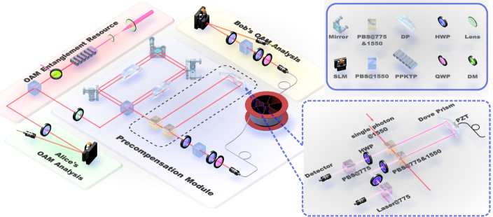
Figure 1: Schematic of the experimental setup. The entangled photons are generated by Type-II SPDC in PPKTP crystal. The idler photon is directly measured (Alice) while the signal photon is fed to a precompensation module and coupled into a 1-kilometer-long OAM fiber and finally analyzed (Bob). The single-photon detectors we use are InGaAs detectors. Here the black dotted box is active locked unbalanced M-Z inteferometer of which the more detailed setup figure is present by the inset. The M-Z inteferometer are both applied to the single photon and classical 775nm reference beam.

We now give more details of the experiment: The entangled photons are produced by degenerate type-II collinear SPDC. Fig. 1 shows the schematic of the experiment. A continuous-wave (CW) 775-nm laser beam is coupled to a single mode fiber (SMF) to obtain a pure fundamental Gaussian mode pump beam. At the output of the SMF, the pump beam is demagnified by a pair of lenses (not shown in Fig. 1) and is incident on a 10-mm-long periodically PPKTP crystal. The power of the pump beam is 36 mw and beam waist on the crystal is $\omega_{0}\backsim 175\,\mu m$. The centre wavelengths of the generated signal and idler photons are $\lambda_{A}{=}\lambda_{B}{=}1550\,nm$, where subscripts A and B refer to Alice and Bob respectively. The pump beam is then blocked by a dichroic mirror.

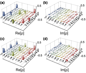
Figure 2: Reconstructed density matrices before ((a), (b)) and after ((c), (d)) distribution. The left column depicts the real part of reconstructed density matrix while the right part depicts the imaginary part. For comparison, the experimental tomographic matrix is drawn with opaque pillars while its closet maximal entangled state (MES) is drawn with transparent pillars.

The OAM state of the photon pairs can be described in terms of Laguerre-Gaussian (LG) modes following

$$\left|\Psi_{SPDC}\right\rangle=\sum_{\ell,\,p_{s},\,p_{i}}C_{\ell,-\ell}^{p_{s},p_{i}}\left|\ell,\,p_{s}\right\rangle\left|-\ell,\,p_{i}\right\rangle$$

where $C_{\ell,-\ell}^{p_{s},p_{i}}$ denotes the complex weightings of the states $\left|\ell,\,p_{s}\right\rangle$ and $\left|-\ell,\,p_{i}\right\rangle$ the quantum state of signal and idler respectively Miatto et al. (2012b). We limit measurements only to $p_{s}{=}p_{i}{=}0$, hence we drop this indices and focus only on the azimuthal mode indices $\ell$: we analyze in the three-dimensional Hilbert space spanned by $\ell=0,\pm 1$. The post-selected state can be written as

$$\left|\Psi_{SPDC}\right\rangle=C_{0,0}\left|0\right\rangle\left|0\right\rangle+C_{1,-1}\left|1\right\rangle\left|-1\right\rangle+C_{-1,1}\left|-1\right\rangle\left|1\right\rangle$$

Here, $C_{0,0},\>C_{1,-1}$ and $C_{-1,1}$ depend on the pump beam profile, crystal length and ratio between pump waist and down-converted beam waist Miatto et al. (2012a, 2011). The quantum state right after the source was reconstructed via standard quantum state tomography using maximum likelihood estimation Thew et al. (2002), we show the density matrix in Fig. 2 (a), (b). The fidelity with respect to three-dimensional MES is $F_{source}{=}0.888\pm 0.007$, and the purity is $P_{source}{=}Tr\left(\rho^{2}\right){=}0.83\pm 0.01$. We note that maximally-entangled states are more easily achieved with thin crystals—these result to a wider spiral spectrum for the same pump characteristics Miatto et al. (2012a) thus leading to states with higher fidelity to an MES. However, thin crystals also result to lesser photon counts that is detrimental to the signal-to-noise ratio, and wider bandwidth not ideal for distribution. We thus chose to generate photons in a PPKTP crystal as in Zhou et al. (2015) to balance the fidelity and photon counts, and also to give a narrower bandwidth. Details of the experimental parameters are shown in Supplementary Materials.

The signal and idler photons are separated by a polarising beamsplitter (PBS). The idler photons are directly analysed by a spatial light modulator (SLM) via phase-flattening measurements Qassim et al. (2014) (Alice in Fig. 1, green region). The signal photon, before going through the 1-km fibre, is fed to the precompensation module, (red region in Fig. 1). This part is critical in the experiment because the intermodal dispersion among different OAM modes acts as a dephasing channel, inevitably leading to decoherence. Therefore, high-dimensional superpositions and entanglement would be destroyed in a few centimeters Löffler et al. (2011); Kang et al. (2012). This is contrast to deterministic transmission of classical OAM information, where one can simply tune the electrical delay to compensate for the delays of the different modes.

We experimentally determine the intermodal dispersion and devise a setup to reverse it, to pre-compensate before entering the 1-km fiber (blue region in Fig. 1). The precompensation module consists of two cascaded interferometers and a locking system. The first interferometer is an OAM sorter which serves as a parity check to convert the different OAM to polarisation according to their topological charge $\ell$. We redesigned the OAM sorter from the Mach-Zehnder configuration Zhang et al. (2014) into a Sagnac interferometer for more robust phase stability. A half wave plate (HWP) is used to rotate the polarisation of signal photon into $\left(\left|H\right\rangle+\left|V\right\rangle\right)/\sqrt{2}$ before entering the OAM sorter. This first interferometer is designed such that OAM modes with odd topological charge ($\ell{=}\pm 1$) are converted to horizontal polarization, and the even ones $\left(\ell=0\right)$ are converted to vertical. The second interferometer is an unbalanced Mach-Zehnder (MZ) interferometer designed to separate the different OAM modes into unequal path lengths: the odd OAM modes enter the short arm and even ones enter the long arm. A dove prism in the long arm is mounted on a translation stage for arm-length tuning to compensate for the intermodal dispersion. To stabilise the path difference between the long and short arms, a phase locking system is used (depicted in Fig. 1 inset). This is composed of a 775 nm laser beam, two photodetectors, and a PZT (piezoelectric transducer) mounted dove prism. Here the phase between the two arms is locked by a 775 nm classical light separated from the pump laser beam. The power of reference light fed into U-shape interferometer is monitored by a tunable beam splitter consisting of a HWP, a PBS at 775 nm and a detector. Both the single photons and the reference 775 nm beam go through the unbalanced MZ inteferometer, the PBSs at the input and output works for both 775 nm and 1550 nm. A HWP ($22.5^{\circ}$) and PBS combined with the detector at the output of laser beam acquire the feedback power signal. Any fluctuation in path difference perturbs the relative phase between $\left|0\right\rangle$ and $\left|\pm 1\right\rangle$ which could be tracked through the readout of the detector. The feedback power signal drives the PZT to stabilize the phase relation with the help of the proportional-integral-derivative (PID) control module. After the cascaded interferometer the single photon is sent to a half-waveplate (HWP) and a polarizing beamspliter (PBS) to erase any polarisation information.

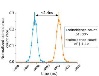
Figure 3: Intermodal dispersion. The normalized coincidence rate is the ratio between each measured coincidence rate and their sum. The horizontal coordinate represents the optical delay between the signal and idler photons. The blue dots represent the coincidence rates for of $\left|0,0\right\rangle$ and the orange dots are for $\left|-1,1\right\rangle$. The intermodal dispersion is estimated by taking the difference in time of the peaks of the Gaussian fits (solid line).

After precompensation, the signal photon is coupled into a 1 km long home-designed step-index fibre which supports OAM modes with $\ell=0,\,\pm 1,\,\pm 2$ (see supplementary material for details on the fibre). The signal photon is then sent to an SLM for analysis (Bob in Fig.1, yellow region). Because the intermodal dispersion varies as the temperature fluctuates, we put the step-index fibre in a sealed adiabatic box with the temperature fluctuation controlled to within $\pm 0.01$ K. Finally, the signal photons are detected over a 0.5 nm bandwidth in Bob’s analysis setup.

We obtain the intermodal dispersion by tuning the delay time of the coincidence module and observing the interval between two coincidence count events ($\left|0,0\right\rangle$ and $\left|-1,1\right\rangle$), found to be 2.4 ns (See Fig. 3 ). The accuracy of this is subject only to the temporal resolution of coincidence module (156 ps), time jitter only broadens the shape of the coincidence curves but does not alter the interval of their peaks.

III CHARACTERIZATION AND CERTIFICATION OF HIGH-DIMENSION NONLOCALITY

The reconstructed density matrix of the entangled state after the signal photon goes through the fibre is presented in Fig. 2(c), (d). The 81 measurement settings required for quantum tomography are represented by projectors $p_{i}\otimes p_{j}(i=1,2,\ldots,9)$, where $p_{k}=\left|\varphi_{k}\right\rangle\left\langle\varphi_{k}\right|$. $\left|\varphi_{k}\right\rangle$ is selected from the following set: $\{\left|-1\right\rangle$, $\left|0\right\rangle$, $\left|1\right\rangle$, $\left(\left|0\right\rangle+\left|-1\right\rangle\right)/\sqrt{2}$, $\left(\left|0\right\rangle+\left|1\right\rangle\right)/\sqrt{2}$, $\left(\left|0\right\rangle+i\left|-1\right\rangle\right)/\sqrt{2}$, $\left(\left|0\right\rangle-i\left|1\right\rangle\right)/\sqrt{2}$, $\left(\left|-1\right\rangle+\left|1\right\rangle\right)/\sqrt{2}$, $\left(\left|-1\right\rangle+i\left|1\right\rangle\right)/\sqrt{2}\}$Thew et al. (2002).

To confirm the quality of the distributed entanglement, we evaluate the fidelity with respect to the three-dimensional MES. The MES can be represented by

$$\left|\Psi_{MES}\left(\theta,\varphi\right)\right\rangle=\left(e^{i\theta}\left|-1\right\rangle\left|1\right\rangle+\left|0\right\rangle\left|0\right\rangle+e^{i\varphi}\left|1\right\rangle\left|-1\right\rangle\right)/\sqrt{3}$$

with different values of $\theta$ and $\varphi$ corresponding to different MESs. We performed a global search for the MES that would give the highest fidelity. With $\theta{=}0.98\times 2\pi$ and $\varphi{=}0.07\times 2\pi$ we obtain a fidelity $F=\left\langle\Psi_{MES}\left(\theta,\varphi\right)\right|\rho\left|\Psi_{MES}\left(\theta,\varphi\right)\right\rangle=0.71\pm 0.02$, and purity $P=Tr\left(\rho^{2}\right)=0.56\pm 0.03$.

This fidelity suffices to certify entanglement beyond two dimension Fickler et al. (2014a), since the overlap between the obtained state with respect to ideal three-dimensional MES cannot be achieved by an entangled state with lower than three dimensions (see Supplementary Material). To further illustrate three-dimensional entanglement we violated a generalized Bell inequality, the Collins-Gisin-Linden-Massar-Popescu (CGLMP) inequality, for qutrits.

The Bell expression in three dimension is Collins et al. (2002)

$$I_{3}\equiv +[P\left(A_{1}=B_{1}\right)+P\left(B_{1}=A_{2}+1\right)$$

$$\quad+P\left(A_{2}=B_{2}\right)+P\left(B_{2}=A_{1}\right)]$$

$$-[P\left(A_{1}=B_{1}-1\right)+P\left(B_{1}=A_{2}\right)$$

$$\quad+P\left(A_{2}=B_{2}-1\right)+P\left(B_{2}=A_{1}-1\right)],$$

where

$$P\left(A_{a}=B_{b}+k\right)\equiv\sum_{j=0}^{2}P\left(A_{a}=j,\,B_{b}=j+k\,mod2\right)$$

We searched for the specific measurement settings $A_{1},$ $A_{2}$ and $B_{1}$, $B_{2}$ to maximally violate the inequality, $I_{3}\leq 2$, imposed by local realism. We obtained $I_{3}=2.12\pm 0.04$. The violation exceeds the classical bound by about 3 standard deviations. Bell-type inequalities such as the CGLMP inequality we use can be considered as entanglement witnesses Hyllus et al. (2005), thus the violation that we show sufficiently proves the existence of three-dimensional entanglement.

IV DISCUSSION AND CONCLUSION

In summary, we have distributed OAM entanglement over 1 km of fibre, three orders of magnutide over previous work Löffler et al. (2011); Kang et al. (2012). The challenging task of maintaining a stable phase relation in the entangled state when one photon undergoes evolution in an optical fibre was overcome by: (1) keeping the temperature of the fibre stable to avoid temperature-induced phase fluctuations in the fibre, and (2) precompensating for the intermodal dispersion. For the latter, we redesigned an OAM sorter Zhang et al. (2014) into a Sagnac cofiguration for better phase stability, and used an unbalanced Mach-Zender interferometer to introduce different delays between the $|0\rangle$ and $|{\pm{1}}\rangle$ states. The dispersion between $|1\rangle$ and $|{-1}\rangle$ is extremely small even for 1-km-length fiber and made even more negligible by narrowing the bandwidth of the measurement such that this dispersion becomes negligible compared to the long coherence time. With our measures, we are able to certify three-dimensional entanglement via a fidelity to the the MES of 0.71, and a violation of a CGLMP inequality.

Supplementary Material for : Distribution of high-dimensional orbital angular momentum entanglement at telecom wavelength over 1km of optical fibre

IV.1 Source of OAM-entangled Photons

The orbital angular momentum (OAM) is conserved in the spontaneous parameter down-conversion process (SPDC) and hence SPDC is the most convenient and efficient method to generate high-dimensional OAM entanglement. However, in practice, such a method generates non-maximally entangled states. The fidelity of the generated state to the maximally entangled state (MES) is related to the crystal length $L$, pump waist $\omega_{p}$, signal (idle) photon waist $\omega_{s}$ ($\omega_{i}$) (Miatto et al., 2012a). Generally, thin crystals such as beta barium borate ($\beta-$BBO) lead to states that are closer to the MED owing to the wider quantum spiral spectrum (Torres et al., 2003).

In our experiment, we are limited by our InGaAs detectors, which for 1550 nm have about 12% efficiency. Instead of using a thin bulk crystal like BBO, we used a 10-mm-long periodically poled potassium titanyl phosphate (PPKTP) crystal, which gives us more photon counts and also a narrower spectral bandwidth. The pump beam is demagnified and collimated by a pair of lenses with the focal length $f=125\,mm$ and $f=25.4\,mm$, before it impinges on the PPKTP crystal with a beam waist of $\omega_{p}\sim 175\,\mu m$. After that PPKTP is directly imaged to two SLMs for analysis using a lens with the focal length $f=150\,mm$.

To improve the accuracy, the hologram embedded in the SLM contains intensity and phase modulations(Bolduc et al., 2013). The SLM hologram is given by

$$\Psi\left(\rho,\phi\right)=\mathcal{L}\left(\rho,\phi\right)Mod\left(\mathcal{F}\left(\rho,\phi\right)+2\pi x/\Lambda,2\pi\right),$$ (1)

with the two modulation functions described by,

$$\begin{array}[]{c}\mathcal{L}\left(\rho,\phi\right)=1+\frac{1}{\pi}sinc^{-1}\left(A\right)\\ \mathcal{F}\left(\rho,\phi\right)=\phi\pi\mathcal{L}.\end{array}$$ (2)

Here, $\phi$ and $A$ are the phase and amplitude distribution of desired OAM state respectively; $2\pi x/\Lambda$ denotes the phase of the blazed grating with period of $\Lambda$ along the x coordinates. Here $\mathcal{L}$ is a normalized bounded positive function of amplitude , i.e, $0\leq\mathcal{L}\leq 1$, which corresponds to the mapping of the phase depth to the diffraction efficiencies of the spatially dependent blazing function.

The single mode fiber (SMF) accepts only the fundamental Gaussian mode, and is connected to a single photon detector (SPD). Because the conversion to the fundamental Gaussian mode is not perfect—some intensity remains outside central bright spot of the fundamental mode Qassim et al. (2014)— there is a difference of detecting efficiencies among different OAM states. We carefully adjusted the pair of lenses ($f=125\,mm$) to minimise the differences.

In order to characterize the quality of the entangled source, we calculate the fidelity with respect to a 3*3 maximally entangled state (MES). We performed a global search to find one MES which is closest to the reconstructed quantum state. The MES is described by

$$\left|\varPsi_{MES}\left(\theta,\varphi\right)\right\rangle=e^{i\theta}\left|-1\right\rangle\left|1\right\rangle+\left|0\right\rangle\left|0\right\rangle+e^{i\varphi}\left|1\right\rangle\left|-1\right\rangle$$

With $\theta=1.02\pi$, $\varphi=0.98\pi$, the highest fidelity between the constructed density matrix $\rho$ and $\varPsi_{MES}$ is $\left\langle\varPsi_{MES}\right|\rho\left|\varPsi_{MES}\right\rangle=0.888\pm 0.007$

IV.2 Eigenmodes in Fiber

The OAM modes are not eigenmodes of the step-index fiber, but it is possible to decompose OAM modes into a superposition of eigenmodes in our step-index fiber. For example, we write the $\left|\ell\right|=1$ mode as following

$$\begin{cases}\mathrm{OAM_{\pm 1}^{\pm}}&=\mathrm{HE_{2,1}^{even}}\pm i\mathrm{HE_{2,1}^{odd}}\\ \mathrm{OAM_{\pm 1}^{\mp}}&=\mathrm{TM_{0,1}}\pm i\mathrm{TE_{0,1}}\end{cases}$$

The superscripts $\pm$ over the OAM represent the right(+) or left(-) circular polarization of photonic state. The four vector modes $\mathrm{HE_{2,1}^{even}}$, $\mathrm{HE_{2,1}^{odd}}$, $\mathrm{TM_{0,1}}$ and $\mathrm{TE_{0,1}}$ , designated as $\mathrm{LP_{11}}$ modes in the scalar approximations, are first higher order eigenmodes of which the effective refractive index are nearly degenerate. The two $\mathrm{HE_{21}}$ modes are strictly degenerate and have an effective refractive index $n_{eff}$ distinct from $\mathrm{TE_{01}}$ and $\mathrm{TM_{01}}$. The effective index of $\mathrm{TE_{01}}$ and $\mathrm{TM_{01}}$ are also slightly different. Nevertheless, discrepancy of $n_{eff}$ among these four modes is extremely small.

In our experiment, the four vector modes are all involved. The near- degeneracy of the modes other than the desired modes makes crosstalk likely. Decoherence between $\ell=1$ and $\ell=-1$ is small because of the small intermodal dispersion. In the main text, the precompensation module is used to compensate for intermodal dispersion (2.4 ns) between $\ell=0$ and $\ell=\pm 1$. As for dispersion between $\ell=1$ and $\ell=-1$, we employed a wave-division-multiplexing (WDM) with a 0.5-nm channel bandwidth, making coherent time much larger such that our measurements are insensitive to the dephasing caused by this intermodal dispersion.

Our fibre is a step-index fiber. It has a core radius of ${\sim}9.5\,\mu m$, a cladding radius of ${\sim}62.5\,\mu m$, and a core cladding refractive index difference of ${\sim}5\times 10^{-3}$, same fibre that we used in our previous work (Wu et al., 2017; Xie et al., 2018). This fibre supports four modes groups $\left(\mathrm{LP_{01},\,LP_{11},\,LP_{21},\,LP_{02}}\right)$, but in our work only two modes groups, i.e. $\mathrm{LP_{01}}$ and $\mathrm{LP_{11}}$ , are used. The effective refractive index of the each LP mode $\left(\mathrm{LP_{01},\,LP_{11},\,LP_{21},\,LP_{02}}\right)$, corresponding to the vector core mode $(\mathrm{HE_{11},\,TE_{01},\,HE_{21},\,TM_{01},\,EH_{11},\,HE_{31},\,HE_{12}})$, is calculated using a full-vector finite-element mode solver, and is given in (Wu et al., 2017).

IV.3 Bipartite Witness for D-dimensional Entanglement.

Table 1: tomographic measurement result of distributed state after vortex fiber. The reconsctructed density matrix is presented in main text.

	$\left|-1\right\rangle$	$\left|0\right\rangle$	$\left|1\right\rangle$	$\frac{\left|0\right\rangle+\left|-1\right\rangle}{\sqrt{2}}$	$\frac{\left|0\right\rangle+\left|1\right\rangle}{\sqrt{2}}$	$\frac{\left|0\right\rangle+i\left|-1\right\rangle}{\sqrt{2}}$	$\frac{\left|0\right\rangle-i\left|-1\right\rangle}{\sqrt{2}}$	$\frac{\left|1\right\rangle+\left|-1\right\rangle}{\sqrt{2}}$	$\frac{\left|1\right\rangle-i\left|-1\right\rangle}{\sqrt{2}}$
$\left|-1\right\rangle$	196	9	17	121	8	132	27	137	101
$\left|0\right\rangle$	8	261	9	119	85	66	106	10	5
$\left|1\right\rangle$	24	14	182	26	146	31	146	77	76
$\frac{\left|0\right\rangle+\left|-1\right\rangle}{\sqrt{2}}$	148	85	9	229	44	122	59	72	49
$\frac{\left|0\right\rangle+\left|1\right\rangle}{\sqrt{2}}$	16	115	92	23	162	69	98	49	44
$\frac{\left|0\right\rangle+i\left|-1\right\rangle}{\sqrt{2}}$	101	115	21	84	61	26	96	86	72
$\frac{\left|0\right\rangle-i\left|-1\right\rangle}{\sqrt{2}}$	19	116	72	79	56	82	35	21	42
$\frac{\left|1\right\rangle+\left|-1\right\rangle}{\sqrt{2}}$	127	16	83	51	82	63	105	147	106
$\frac{\left|1\right\rangle-i\left|-1\right\rangle}{\sqrt{2}}$	97	13	86	74	84	76	107	141	23

The 81 measurement settings required for quantum tomography are represented by projectors $p_{i}\otimes p_{j}(i=1,2,\ldots,9)$, where $p_{k}=\left|\varphi_{k}\right\rangle\left\langle\varphi_{k}\right|$. The set of $\left|\varphi_{k}\right\rangle$ is given in the main text. The measurement results are presented in Table 1. We performed quantum state tomography and obtained the fidelity $F$ both before and after distribution. We employed the method developed in (Fickler et al., 2014b) to certify the 3-dimensional entanglement. In the following text, we bound the maximal overlap between the chosen high-dimensional state and states with a bounded Schmidt rank $d$. If the fidelity reveals a higher overlap than this bound, the justification of at least $\left(d+1\right)$-dimensional entanglement is proven.

The Schimidt decomposition of the assumed high-dimensional state is described as $\left|\varphi\right\rangle=\sum_{i=1}^{D}\lambda_{i}\left|ii\right\rangle$ with the coefficients in a decreasing order $\left|\lambda_{1}\right|\geq\left|\lambda_{2}\right|\geq\cdots\geq\left|\lambda_{D}\right|$, where $i$ denotes the different OAM state and $D$ the dimension of the Hilbert space. The witness for $d$-dimensional entanglement is constructed by comparing the two fidelities

$$F = Tr\left(\rho\left|\varphi\right\rangle\left\langle\varphi\right|\right)$$

$$F_{d} = \max_{\phi_{d}}\left|\left\langle\phi_{d}|\varphi\right\rangle\right|^{2}$$

where $\rho$ is the density matrix after distribution and $\left|\phi_{d}\right\rangle=\sum_{m,n=1}^{D}\alpha_{mn}\left|mn\right\rangle$ represents states with a bounded Schmidt rank $d$. The global search for maximizing the $F_{d}$ implies that $F\geq F_{d}$ could not be satisfied by a $d$-dimensional entangled state. In other word, the generated bipartite system is at least $\left(d+1\right)$-dimensionally entangled.

We directly calculate $F_{d}$ as the maximal overlap:

$$F_{d} = \max_{\phi_{d}}\left|\left(\left\langle mn\right|\sum_{m,n=1}^{D}\alpha_{mn}^{\ast}\right)\left(\sum_{i=1}^{D}\lambda_{i}\left|ii\right\rangle\right)\right|^{2}$$

$$= \max_{\phi_{d}}\left|Tr\left(\sum_{i,m,n=1}^{D}\left\langle m|i\right\rangle\left\langle n|i\right\rangle\alpha_{mn}^{\ast}\lambda_{i}\right)\right|^{2}$$

We introduce two operators in the form of

$$U = c_{mn}\left|m\right\rangle\left\langle n\right|$$

$$P_{d}U^{\ast} = U^{\ast}$$

where $P_{d}$ is a rank $d$-projector which always exists if $B^{\ast}$ is of rank d, as $\left|\phi_{d}\right\rangle$ is also of Schmidt rank d. Combining these equations, we have

$$F_{d} = \max_{\phi_{d}}\left|Tr\left(U\dagger\sum_{i=1}^{D}\lambda_{i}\left|i\right\rangle\left\langle i\right|\right)\right|^{2}$$

$$= \max_{\phi_{d}}\left|Tr\left(P_{d}U\dagger\sum_{i=1}^{D}\lambda_{i}\left|i\right\rangle\left\langle i\right|\right)\right|^{2}$$

$$= \max_{\phi_{d}}\left|Tr\left(U\dagger\sum_{i=1}^{D}\lambda_{i}\left|i\right\rangle\left\langle i\right|P_{d}\right)\right|^{2}$$

Note that for the inner product $\left\langle A,B\right\rangle\equiv Tr\left(A,B\dagger\right)$, taking advantage of Cauchy-Schwarz inequality $\left(\left|\left\langle A,B\right\rangle\right|^{2}\leq\left\langle A,A\right\rangle\left\langle B,B\right\rangle\right)$, the upper bound of $F_{d}$ is found to be

$$F_{d}\leq\max_{\phi_{d}}Tr\left(BB\dagger\right)Tr\left(P_{d}\sum_{i=1}^{D}\left|\lambda_{i}\right|^{2}\left|i\right\rangle\left\langle i\right|P_{d}\right).$$

Because $Tr\left(BB\dagger\right)=\sum_{m,n=1}^{D}c_{mn}c_{nm}^{\ast}\leq 1$ and choosing $P_{d}=\sum_{i=1}^{d}\left|i\right\rangle\left\langle i\right|$, we get the upper bound of $F_{d}$ for $d$-dimensional entangled states with a simple fomula

$$F_{d}\leq\sum_{i=1}^{d}\left|\lambda_{i}\right|^{2}$$

By choosing a specific $\left|\phi_{d}\right\rangle=\left(1/\sqrt{\sum_{i=1}^{d}\left|\lambda_{i}\right|^{2}}\right)\sum_{i=1}^{d}\lambda_{i}\left|ii\right\rangle$, we find that

$$F_{d}\geq\sum_{i=1}^{d}\left|\lambda_{i}\right|^{2}$$

Thus we find a tight bound for witness of $\left(d+1\right)$-dimensional entanglement

$$F_{d}=\max_{\phi_{d}}\left|\left\langle\phi_{d}|\varphi\right\rangle\right|^{2}=\sum_{i=1}^{d}\left|\lambda_{i}\right|^{2}$$

For $d=2$, this upper bound is found to be $\frac{2}{3}$. With the fidelity $F=0.71\pm 0.02$ that we experimentally obtained, we conclude that our results can only be explained by a state that is at least three-dimensional entangled state

$$F_{d}>\sum_{i=1}^{d}\left|\lambda_{i}\right|^{2}$$

The witness also holds for mixed state,x which would only lower the bound due to the convexity of fidelity.

IV.4 Quantum Process Tomography

The entire state-transfer process (precompensation and evolution in vortex fiber combined) can be represented by a quantum process $\chi$ (O’Brien et al., 2004). The output state can be described by

$$\rho_{out}=\sum_{m,n=1}^{9}\chi_{mn}\lambda_{m}\rho_{in}\lambda_{n}^{\dagger}$$

where $\rho_{in}$ is the input state and $\lambda_{m}$ is the basis of qutrit operators. The process matrix $\chi$ can be identified by measuring the output $\rho_{in}$ for a series of input state $\rho_{in}$. The input state are chosen from the states set $|\phi_{k}\rangle$ (see Table 1).

The corresponding complete operator basis are presented as follows Thew et al. (2002): $\lambda_{1}{=}\left\{\begin{array}[]{ccc}1&0&0\\ 0&1&0\\ 0&0&1\end{array}\right\},\lambda_{2}{=}\left\{\begin{array}[]{ccc}0&1&0\\ 1&0&0\\ 0&0&0\end{array}\right\}$,$\lambda_{3}{=}\left\{\begin{array}[]{ccc}0&-i&0\\ i&0&0\\ 0&0&0\end{array}\right\}$,
$\lambda_{4}{=}\left\{\begin{array}[]{ccc}1&0&0\\ 0&-1&0\\ 0&0&0\end{array}\right\}$,$\lambda_{5}{=}\left\{\begin{array}[]{ccc}0&0&1\\ 0&0&0\\ 1&0&0\end{array}\right\}$,$\lambda_{6}{=}\left\{\begin{array}[]{ccc}0&0&-i\\ 0&0&0\\ i&0&0\end{array}\right\}$,
$\lambda_{7}{=}\left\{\begin{array}[]{ccc}0&0&0\\ 0&0&1\\ 0&1&0\end{array}\right\}$,$\lambda_{8}{=}\left\{\begin{array}[]{ccc}0&0&0\\ 0&0&-i\\ 0&i&0\end{array}\right\}$,
$\lambda_{9}{=}\left\{\begin{array}[]{ccc}1&0&0\\ 0&1&0\\ 0&0&-2\end{array}\right\}/\sqrt{3}$.

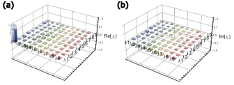
Figure 4: Process matrix of state transfer process (combination of precompensation and inside-fiber evolution). (a) and (b) represent the real and imaginary part of process matrix respectively, with the opaque histogram denoting the experimental tomographic matrix and transparent histogram denoting the ideal identity matrix $\chi_{0}=\mathcal{I}$.

For an ideal situation, the state transfer process should be an identity matrix $\chi_{0}=\mathcal{I}$, regardless of the phase shift in fiber which could be removed by redefining the qutrit basis. Here we applied the process tomography to the state-transfer process. A wide bandwidth attenuated laser pass the wave division multiplexing to narrow the bandwidth to 0.5 nm (as in the main text), the attenuated single photons are emitted from the coupler in Alice’s part, and sent to the SLM for input state preparation. The PPKTP was replaced by a mirror, and the photons were sent in the reverse direction (from Alices’s detector side to mirror). The mirror reflects the photon into the arm of the precompensation module where. The reconstructed process matrix $\chi$ is shown in Fig.4. The fidelity is calculated by $F=\left[\mathrm{Tr}\left(\sqrt{\sqrt{\chi}\chi_{0}\sqrt{\chi}}\right)\right]^{2}=0.747$. The process is different from identity, which would have been the case ideally. The discrepancy comes from several factors: According to our experiment data, there still is 12.8% crosstalk between the OAM modes. This crosstalk comes from the mode mismatch in the optical fibre. As is discussed above, in our experiment three OAM modes ($\ell=0,\pm 1$) relate to six eigenstate of $LP_{00}$ and $LP_{11}$ mode groups in the fiber, crosstalk between degenerate or near degenerate state is likely. The spatial mode is also sensitive to any imperfections in the optical surfaces. This affects mode matching into the fibre. These factors causes are all experimental imperfections rather than a drawback of our method in principle.

References

- Fujiwara et al. (2003) M. Fujiwara, M. Takeoka, J. Mizuno, and M. Sasaki, Physical review letters 90, 167906 (2003).
- Bechmann-Pasquinucci and Tittel (2000) H. Bechmann-Pasquinucci and W. Tittel, Physical Review A 61, 062308 (2000).
- Gisin et al. (2002) N. Gisin, G. Ribordy, W. Tittel, and H. Zbinden, Reviews of modern physics 74, 145 (2002).
- Aolita and Walborn (2007) L. Aolita and S. Walborn, Physical review letters 98, 100501 (2007).
- Ali-Khan et al. (2007) I. Ali-Khan, C. J. Broadbent, and J. C. Howell, Physical review letters 98, 060503 (2007).
- D’Ambrosio et al. (2012) V. D’Ambrosio, E. Nagali, S. Walborn, L. Aolita, S. Slussarenko, L. Marrucci, and F. Sciarrino, Nature communications 3, 961 (2012).
- Nunn et al. (2013) J. Nunn, L. Wright, C. Söller, L. Zhang, I. Walmsley, and B. Smith, Optics express 21, 15959 (2013).
- Mower et al. (2013) J. Mower, Z. Zhang, P. Desjardins, C. Lee, J. H. Shapiro, and D. Englund, Physical Review A 87, 062322 (2013).
- Graham et al. (2015) T. M. Graham, H. J. Bernstein, T.-C. Wei, M. Junge, and P. G. Kwiat, Nature communications 6 (2015).
- Langford et al. (2004) N. K. Langford, R. B. Dalton, M. D. Harvey, J. L. O’Brien, G. J. Pryde, A. Gilchrist, S. D. Bartlett, and A. G. White, Physical review letters 93, 053601 (2004).
- Dada et al. (2011) A. C. Dada, J. Leach, G. S. Buller, M. J. Padgett, and E. Andersson, Nature Physics 7, 677 (2011).
- Romero et al. (2012) J. Romero, D. Giovannini, S. Franke-Arnold, S. Barnett, and M. Padgett, Physical Review A 86, 012334 (2012).
- Giovannini et al. (2013) D. Giovannini, J. Romero, J. Leach, A. Dudley, A. Forbes, and M. J. Padgett, Physical review letters 110, 143601 (2013).
- Krenn et al. (2014) M. Krenn, M. Huber, R. Fickler, R. Lapkiewicz, S. Ramelow, and A. Zeilinger, Proceedings of the National Academy of Sciences 111, 6243 (2014).
- Malik et al. (2016) M. Malik, M. Erhard, M. Huber, M. Krenn, R. Fickler, and A. Zeilinger, Nature Photonics 10, 248 (2016).
- Collins et al. (2002) D. Collins, N. Gisin, N. Linden, S. Massar, and S. Popescu, Physical review letters 88, 040404 (2002).
- Löffler et al. (2011) W. Löffler, T. Euser, E. Eliel, M. Scharrer, P. S. J. Russell, and J. Woerdman, Physical review letters 106, 240505 (2011).
- Kang et al. (2012) Y. Kang, J. Ko, S. M. Lee, S.-K. Choi, B. Y. Kim, and H. S. Park, Physical review letters 109, 020502 (2012).
- Luo et al. (2019) Y.-H. Luo, H.-S. Zhong, M. Erhard, X.-L. Wang, L.-C. Peng, M. Krenn, X. Jiang, L. Li, N.-L. Liu, C.-Y. Lu, et al., Phys. Rev. Lett. 123, 070505 (2019).
- Hu et al. (2019) X.-M. Hu, C. Zhang, B.-H. Liu, Y.-F. Huang, C.-F. Li, and G.-C. Guo, arXiv preprint arXiv:1904.12249 (2019).
- Kues et al. (2017) M. Kues, C. Reimer, P. Roztocki, L. R. Cortés, S. Sciara, B. Wetzel, Y. Zhang, A. Cino, S. T. Chu, B. E. Little, et al., Nature 546, 622 (2017).
- Ikuta and Takesue (2018) T. Ikuta and H. Takesue, Scientific reports 8, 817 (2018).
- Steinlechner et al. (2017) F. Steinlechner, S. Ecker, M. Fink, B. Liu, J. Bavaresco, M. Huber, T. Scheidl, and R. Ursin, Nature communications 8, 15971 (2017).
- Lee et al. (2017) H. J. Lee, S.-K. Choi, and H. S. Park, Scientific reports 7, 4302 (2017).
- O’neil et al. (2002) A. O’neil, I. MacVicar, L. Allen, and M. Padgett, Physical review letters 88, 053601 (2002).
- Fickler et al. (2016) R. Fickler, G. Campbell, B. Buchler, P. K. Lam, and A. Zeilinger, Proceedings of the National Academy of Sciences 113, 13642 (2016).
- Wang et al. (2017) F. Wang, M. Erhard, A. Babazadeh, M. Malik, M. Krenn, and A. Zeilinger, Optica 4, 1462 (2017).
- Kong et al. (2019) L.-J. Kong, R. Liu, Z.-X. Wang, Y. Si, W.-R. Qi, S.-Y. Huang, C. Tu, Y. Li, W. Hu, F. Xu, et al., Science Advances 5, eeat9206 (2019).
- Babazadeh et al. (2017) A. Babazadeh, M. Erhard, F. Wang, M. Malik, R. Nouroozi, M. Krenn, and A. Zeilinger, Physical review letters 119, 180510 (2017).
- Erhard et al. (2017) M. Erhard, M. Malik, M. Krenn, and A. Zeilinger, arXiv preprint arXiv:1708.03881 (2017).
- Krenn et al. (2015) M. Krenn, J. Handsteiner, M. Fink, R. Fickler, and A. Zeilinger, Proceedings of the National Academy of Sciences 112, 14197 (2015).
- Cozzolino et al. (2019) D. Cozzolino, D. Bacco, B. Da Lio, K. Ingerslev, Y. Ding, K. Dalgaard, P. Kristensen, M. Galili, K. Rottwitt, S. Ramachandran, et al., Physical Review Applied 11, 064058 (2019).
- Capenter et al. (2013) J. Capenter, C. Xiong, M. J. Collins, J. Li, T. F. Krauss, and B. J. Eggleton, Optics Express 21, 28794 (2013).
- Torres et al. (2003) J. Torres, A. Alexandrescu, and L. Torner, Physical Review A 68, 050301 (2003).
- Miatto et al. (2012a) F. Miatto, D. Giovannini, J. Romero, S. Franke-Arnold, S. Barnett, and M. Padgett, The European Physical Journal D-Atomic, Molecular, Optical and Plasma Physics 66, 1 (2012a).
- Miatto et al. (2012b) F. M. Miatto, H. D. L. Pires, S. M. Barnett, and M. P. van Exter, The European Physical Journal D 66, 263 (2012b).
- Miatto et al. (2011) F. M. Miatto, A. M. Yao, and S. M. Barnett, Physical Review A 83, 033816 (2011).
- Thew et al. (2002) R. Thew, K. Nemoto, A. G. White, and W. J. Munro, Physical Review A 66, 012303 (2002).
- Zhou et al. (2015) Z.-Q. Zhou, Y.-L. Hua, X. Liu, G. Chen, J.-S. Xu, Y.-J. Han, C.-F. Li, and G.-C. Guo, Physical review letters 115, 070502 (2015).
- Qassim et al. (2014) H. Qassim, F. M. Miatto, J. P. Torres, M. J. Padgett, E. Karimi, and R. W. Boyd, JOSA B 31, A20 (2014).
- Zhang et al. (2014) W. Zhang, Q. Qi, J. Zhou, and L. Chen, Physical review letters 112, 153601 (2014).
- Fickler et al. (2014a) R. Fickler, R. Lapkiewicz, M. Huber, M. P. Lavery, M. J. Padgett, and A. Zeilinger, Nature Communications 5 (2014a).
- Hyllus et al. (2005) P. Hyllus, O. Gühne, D. Bruß, and M. Lewenstein, Physical Review A 72, 012321 (2005).
- Bolduc et al. (2013) E. Bolduc, N. Bent, E. Santamato, E. Karimi, and R. W. Boyd, Optics letters 38, 3546 (2013).
- Wu et al. (2017) H. Wu, S. Gao, B. Huang, Y. Feng, X. Huang, W. Liu, and Z. Li, Optics letters 42, 5210 (2017).
- Xie et al. (2018) Z. Xie, S. Gao, T. Lei, S. Feng, Y. Zhang, F. Li, J. Zhang, Z. Li, and X. Yuan, Photonics Research 6, 743 (2018).
- Fickler et al. (2014b) R. Fickler, R. Lapkiewicz, M. Huber, M. P. Lavery, M. J. Padgett, and A. Zeilinger, Nature communications 5, 4502 (2014b).
- O’Brien et al. (2004) J. L. O’Brien, G. Pryde, A. Gilchrist, D. James, N. K. Langford, T. Ralph, and A. White, Physical review letters 93, 080502 (2004).