Performance Analysis of Deep Learning based on Recurrent Neural Networks for Channel Coding

Abstract

Channel Coding has been one of the central disciplines driving the success stories of current generation LTE systems and beyond. In particular, turbo codes are mostly used for cellular and other applications where a reliable data transfer is required for latency-constrained communication in the presence of data-corrupting noise. However, the decoding algorithm for turbo codes is computationally intensive and thereby limiting its applicability in hand-held devices. In this paper, we study the feasibility of using Deep Learning (DL) architectures based on Recurrent Neural Networks (RNNs) for encoding and decoding of turbo codes. In this regard, we simulate and use data from various stages of the transmission chain (turbo encoder output, Additive White Gaussian Noise (AWGN) channel output, demodulator output) to train our proposed RNN architecture and compare its performance to the conventional turbo encoder/decoder algorithms. Simulation results show, that the proposed RNN model outperforms the decoding performance of a conventional turbo decoder at low Signal to Noise Ratio (SNR) regions.

I Introduction

The 5G wireless networks are a major transformational force that is propelled by the explosion of radio devices along with advanced and not yet supported applications and services spanning across multiple domains such as industrial and vehicular communications. Beyond the need for high data rates, a factor that has been the primary driver for the evolution of wireless networks until 4G, 5G networks should also be able to support diverse Quality of Service (QoS) requirements such as Ultra Reliable Low Latency Communication (URLLC), Massive Machine Type Communications (MMTC) etc. Added to this, the Internet of Things (IoT) ecosystem would necessitate collecting short packets of periodic data in real time thus leading to substantial traffic on the uplink channel. These new applications also bring with them complex scenarios with unknown channel models, high speed and accurate processing requirements [1]; thereby challenging conventional communication system algorithms and hence paving the way for a paradigm shift in the design of communication systems.

Driven by this demand, Machine Learning (ML), which has shown substantial promises during recent years[2] is extensively studied by researchers in order to assess its applicability to wireless networks. Deep Learning (DL), which belongs to a class of ML algorithms, that uses multiple layers of non linear processing units stacked on top of each other. Each successive layer uses the output of the previous layer as input. Such DL architectures are especially suitable for designing auto encoders that aim to find a low-dimensional representation of its input at some intermediate layer that allows reconstruction at the output with minimal error. DL architectures such as Convolutional Neural Networks (CNNs), RNNs, Generative Adversarial Networks (GANs), Deep Belief Networks (DBNs) have been applied to various domains such as computer vision, natural language processing, social network filtering, drug design etc. where they have produced results comparable to and in some cases superior to human experts.

Initially applied to upper layers, such as resource management[3], link adaptation[4, 5], obstacle detection [6] and localization[7], ML has recently found applications also at the Physical Layer (PHY) functions such as channel coding[8, 9], modulation recognition[10, 11], physical layer security [12], and channel estimation and equalization[13, 14] etc.

The first attempts for using Artificial Neural Networks (ANNs) for decoding turbo codes were presented in [15] where the author proposes an ANN based on Multi Layer Perceptrons (MLPs). With the advent of training techniques such as layer-by-layer unsupervised pre-training followed by gradient descent fine-tuning and back propagation, the interest for using ANNs for channel coding is renewed. Different ideas around the use of ANNs for decoding emerged in the 1990s with works such as [16, 17, 18] for decoding block and hamming codes. Subsequently, ANNs were used for decoding convolutional codes in [19, 20]. In [21], the author used MLPs to generate Low-Density Parity-Check (LDPC) codes. More recent works such as [22] use the more advanced deep ANNs for decoding structured polar codes.

In this work, we investigate DL architectures to design and analyse an ANN for turbo coding and decoding operations that are typically performed at the PHY. Specifically, we use the turbo encoder and decoder variant specified for LTE [23]. To this end, we frame the encoding and decoding operations as a supervised learning problem and use a RNN architecture to autoencode-decode the data and compare its performance in terms of Bit Error Rate (BER) to the legacy LTE turbo encoding/decoding blocks. Our motivation is two fold

1. Traditional signal processing is done by logically separated blocks that are independently optimized to recover the data signal from imperfect channels. Although this approach is perfected over many years, it may not achieve the optimal end-to-end performance. A well learned DL encoder/decoder is by default optimized for end-to-end performance.

2. ANNs are shown to be universal function approximators[24] and are known to be Turing complete[25]. Their execution can be highly parallelized on distributed memory architectures such as Graphical Processing Units (GPUs) that have high energy efficiency and computational throughput. Hence, these learned algorithms could be executed faster and at lower energy cost than traditional signal processing blocks.

This work is organized as follows. Section II presents a brief overview of the turbo encoding and decoding operations used in LTE. A general introduction to DL and RNNs is presented in Section III. Section IV explains the problem formulation, data preparation, model architecture and the training operation with the corresponding numerical results presented in Section V. Section VI concludes the paper and presents some discussions for future work.

II Turbo Encoder Architecture and Interfaces

In general sense, a turbo encoder consists of two encoders (referred to as constituent encoders) separated by an interleaver. The encoders are normally identical and the interleaver is used to scramble the bits before being fed to the second encoder. Thus the encoder outputs are different from each other. LTE uses two 8-state identical Recursive Systematic Convolutional (RSC) encoders that are concatenated in parallel and separated by an internal interleaver [23] as shown in Fig. 1.

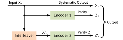
Figure 1: Turbo Encoder Architecture

The transfer function of each constituent encoder is given as

$$G(D)=\begin{bmatrix}1,\frac{g_{1}(D)}{g_{0}(D)}\end{bmatrix}$$

where $g_{0}(D)=1+D^{2}+D^{3}$ and $g_{1}(D)=1+D+D^{3}$

For a given input bit stream $X_{0},X_{1},...,X_{K-1}$ of length $K$, the output of the turbo encoder is given as

$$X_{0},Z_{0},Z^{\prime}_{0},X_{1},Z_{1},Z^{\prime}_{1},...,X_{K-1},Z_{K-1},Z^{\prime}_{K-1}$$

where

1. Bits $X_{0},X_{1},...,X_{K-1}$ are the systematic bits as well as the input to the first constituent encoder and the internal interleaver

2. Bits $Z_{0},Z_{1},...,Z_{K-1}$ and $Z^{\prime}_{0},Z^{\prime}_{1},...,Z^{\prime}_{K-1}$ are outputs from the first an second constituent encoders

As can be seen from the Fig. 1, bits $X^{\prime}_{0},X^{\prime}_{1},...X^{\prime}_{K-1}$ are outputs from the internal interleaver (and the input to the second constituent encoder) for which the relationship between input and output bits is given as

$$X^{\prime}_{i}=X_{\pi(t)},\>i=0,1,...,K-1$$

where the relationship between the output index $i$ and the input index, $\pi(i)$ satisfies the following quadratic form

$$\pi(i)=(f_{1}i+f_{2}i^{2})$$

where parameters $f_{1}$ and $f_{2}$ depend on the block size $K$. The valid block lengths along with their corresponding $f_{1}$, $f_{2}$ values are given in the 3GPP specification [23].

Each bit stream is trellis terminated, by taking the tail bits from the shift register after encoding and padding them to the stream bits. This is done so as to reset the encoder state to zero after every encoding operation. Hence, for any given $k$ bits, the output length of the turbo encoder is $3*k+3*m$ where $m$ is the memory size in the shift registers. For LTE variant, the size of $m$ is 4 and hence 4 tail bits are added to each stream totalling 12 bits.

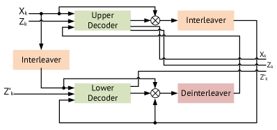
Figure 2: Turbo Decoder Architecture

At the receiver end, the turbo decoder consists of two single soft-in soft-out (SISO) decoders that work iteratively. As seen from Fig. 2, the output of the upper decoder feeds into the lower decoder to form a turbo decoding iteration. Interleaver and deinterleaver blocks re-order data in this process. Two decoding algorithms based on Maximum A Posteriori (MAP), namely LogMAP and MaxLogMAP are used for the decoding process.

III Deep Learning for Turbo Encoding and Decoding

Any ML algorithm learns the execution of a particular task $T$, maintaining a specific performance metric $M$, based on exploiting its experience $E$[26]. ML algorithms can be classified into Supervised and Unsupervised depending on the presence/absence of labeled samples in the input dataset. DL is an emerging algorithm belonging to the class of ANNs which consists of multiple stacked layers with each layer consisting of an arbitrary number of neurons. At each neuron, all of its weighted inputs are added up along with a bias and the result is propagated to the next layer through a nonlinear activation function. Each layer $i$ with $n_{i}$ inputs and $m_{i}$ outputs performs a mapping $f^{(i)}:\mathbb{R}^{n_{i}}\mapsto\mathbb{R}^{m_{i}}$. Denoting $r_{o}$ as output and $r_{i}$ as input of the ANN, the input-output mapping is defined by a chain of functions depending on the parameter set $\theta$ (weights and biases) by

$$r_{o}=f(r_{i};\theta)=f^{(L-1)}\left(f^{(L-2)}\left(...\left(f^{(0)}(r_{i})\right)\right)\right)$$

where $L$ is the number of layers in the ANN (also referred to as depth). In order to find the optimal weights of the ANN, a training operation with a specific loss function is defined. During training, the ANN adjusts its weights to minimize the loss function over the training set by means of gradient descent optimization methods and the backpropagation algorithm.

ANNs can be broadly classified into two types - feed forward networks where the information moves only in the forward direction from input nodes, through the hidden nodes and to the output nodes. Examples of such ANN architectures include a simple perceptron, CNNs. These are suitable for learning unconnected inputs such as image / video processing. In this paper, we are dealing with turbo encoding and decoding operations that exhibit temporal dependencies between input sequences. Hence, our discussion is limited to RNNs that are better suited to learning connected inputs. Unlike traditional feed forward networks, RNNs have an internal hidden state (memory) whose activation at each time is dependent on that of the previous time and are hence suitable to process connected input sequences. Formally, given a sequence $(x_{1},x_{2},...,x_{T})$, the RNN updates its recurrent hidden state $h_{t}$ as follows

$$h_{t}=g(Wx_{t}+Uh_{t-1})$$

where $g$ is a smooth, bounded non-linear function (e.g., sigmoid function), and $W$, $U$ are parameters of the network.

Out of many available RNNs, two variants stand out. The first is based on Long-Short Term Memory (LSTM) [27] and the second one is based on the more recent Gated Recurrent Unit (GRU) [28]. The key difference between them is that LSTM uses three gates (namely input, output and forget gates) whereas GRU uses two gates (reset and update gates). The flow of information is similar for both the architectures except that GRU does not use a memory unit and exposes the full hidden content without any control. The performance of GRU is almost on par with LSTM albeit at a lower computational complexity. It is because of these reasons that we select GRUs as the underlying units for our proposed RNN.

III-A Gated Recurrent Unit (GRU)

GRU was proposed in [28] to make each unit to adaptively capture dependencies of different time scales. The activation $h_{t}$ of a GRU at time $t$ is a linear interpolation between the previous activation $h_{t-1}$ and the target activation $\tilde{h}_{t}$

$$h_{t}=(1-z_{t})h_{t-1}+z_{t}\tilde{h}_{t}$$

where the update gate $z_{t}$ decides how much the unit updates it activation and is computed as

$$z_{t}=\tanh(Wx_{t}+U(r_{t}\odot h_{t-1}))^{j}$$

where $\odot$ is an elementwise multiplication and $r_{t}$ is a set of reset gates that are computed similarly to the update gates as

$$r_{t}=\sigma(W_{r}x_{t}+U_{r}h_{t-1})^{j}$$

III-B Activation Function

The activation used in all the models is a sigmoid function to induce non-linearity to the outputs and also due to its good binary classification capability. It is a special case of a logistic function and is defined by the formula

$$S(x)=\frac{1}{1+e^{-x}}$$

III-C Cost Funtion

The cost or loss function is used to evaluate the performance of a given network and update the weights accordingly. Due to the binary nature of our activation function, we selected binary cross-entropy as the loss function which can be calculated as

$$f(l)=-(y\log(p))+(1-y)\log(1-p)$$

where $y$ is the binary indicator (0 or 1) if the output value is equal to the true value and $p$ is the predicted probability of an observation being either 0 or 1.

III-D Optimizer

For all the models, Adaptive Moment Estimation (ADAM) optimizer was used. It computes the learning rates by calculating an exponentially decaying average of past gradients $m_{t}$ in addition to past squared gradients $v_{t}$ as follows[29]

$$\begin{split}m_{t}&=\beta_{1}m_{t-1}+(1-\beta_{1})g_{t}\\ v_{t}&=\beta_{2}v_{t-1}+(1-\beta_{2})g^{2}_{t}\end{split}$$

These values are then used to update the weights according to following rule

$$\theta_{t+1}=\theta_{t}-\frac{\eta}{\sqrt{v_{t}}+\epsilon}m_{t}$$

IV Simulation Framework

In this work, we investigate the performance of RNNs based on GRUs for encoding and decoding of turbo codes. In order to train the model, data was generated using the communications system toolbox in Matlab and the sequence of operations are highlighted in Fig. 3

IV-A Problem Formulation, Data Generation & Preparation

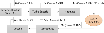
Figure 3: Simulation Method

A total of four autoencoding problems have been formulated - one for encoding and the remaining three for decoding as follows.

IV-A1 Turbo Encoding

A series of binary bits are given as input to the RNN whose goal is to encode them by adding redundancy and output the turbo encoded bits. 10000 packets of size 64 bits were generated i.e., $\text{size}(x_{i})=(10000,64)$ as input and we used the LTE variant of turbo encoder to encode the data. Because of the trellis termination, tail bits are added to each data stream thus creating the resulting encoded data $x_{e}$ of size $(10000,204)$. No AWGN noise is considered for this scheme.

IV-A2 Turbo Decoding

For the turbo decoding, three data generation approaches were considered

1. Reversing the $x_{i}$ and $x_{e}$ obtained from the previous step and feeding the encoded data $x_{e}$ to the RNN to obtain the decoded bits $x_{i}$. This is the simplest case without considering any noise and modulation.

2. Using the demodulated soft bits $x_{dm}$ which is fed to the RNN in-order to obtain the decoded bits $x_{i}$. Data is generated for different SNRs in range [-2,2) totalling 11*10000 = 110000 samples.

3. Using the noise affected data $x_{n}$ which is of complex data type directly without demodulation and feeding it as input to the RNN to obtain the decoded bits $x_{i}$. Similar to the second approach, data is generated for different SNRs in the range [-2,2) totalling 110000 samples.

For each auto-encoding problem, we shuffle and split the input data into training and testing datasets in the ratio of 30%-70% respectively. No scaling/preprocessing has been used.

IV-B RNN Model, Training & Validation

TABLE I: Model Architecture

(a) Input Shapes

Problem	Input Shape	Output Shape
Turbo Encoding	($N_{s}$, 1, 64)	($N_{s}$, 204)
Turbo Decoding - 1	($N_{s}$, 1, 204)	($N_{s}$, 64)
Turbo Decoding - 2	($N_{s}$, 1, 204)	($N_{s}$, 64)
Turbo Decoding - 3	($N_{s}$, 2, 204 / m*)	($N_{s}$, 64)
$N_{s}$ is batch size
*m = 2,4,6 for QPSK, 16QAM and 64QAM

(b) Layers

Layer	Shape	Parameters
Input	Refer to I(a)	None
GRU- 1	($N_{s}$,1,800)	2078400
Batch Normalization - 1	($N_{s}$,1,800)	3200
GRU- 2	($N_{s}$,800)	3844800
Batch Normalization - 2	($N_{s}$,800)	3200
Dense	Refer to I(a)	Variable
Total Trainable Parameters $\approx$ 6,000,000

The model used in this work is similar to the one presented in [30] and can be seen in Table I(b). It consists of two layers of bidirectional GRUs with each layer followed by a batch normalization layer. The output layer is a single fully connected sigmoid unit. The bi-directionality is intended to support recursion in both forward pass and backward pass through the received sequence. It has to be noted that the same model is used for all the autoencoding problems by modifying the input shape (Table I(a))

The training set is further split into model training and validation datasets in the ratio of 90%-10%. The model is trained on the training dataset on an Nvidea GPU for 30 epochs (an epoch is one pass over the entire dataset) and validated on the validation set. Finally, the model is applied on the testing dataset.

V Results

For problem sets 1 and 2, the training, validation and testing accuracies for a single SNR point were used for performance evaluation since there is no noise added to the input data. For problem set 3 and 4, the testing BER $(1-\text{testing accuracy})$ per SNR point was used.

V-A Turbo Encoding and Decoding on data with no noise

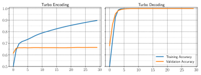
Figure 4: Training & Validation Accuracy - No Noise

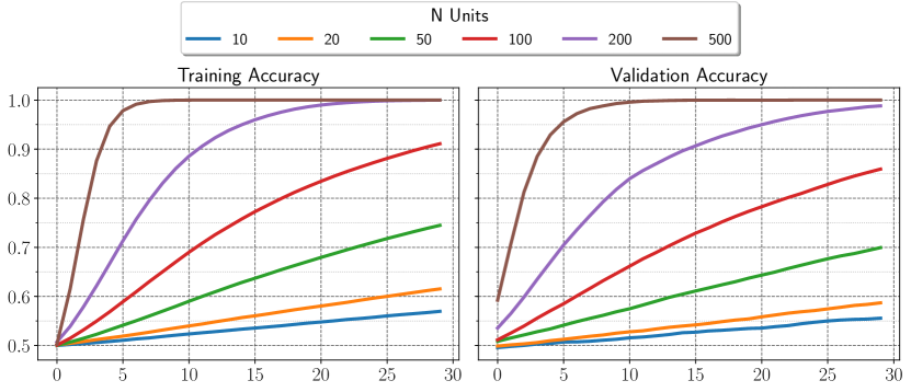
(a) Effect of Number of GRU Units on Accuracy

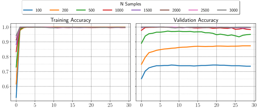
(b) Effect of Number of training samples on Accuracy

Figure 5: Model Selection & Validation

Fig. 4 shows the training accuracy of the model over number of epochs for the turbo encoding and decoding performance without any noise (Problem 1 and 2). In case of encoding, even though the model shows a high training accuracy, the validation accuracy stays constant at 67% after 3 epochs. On the contrary, the model performs well for decoding the turbo codes with training and validation accuracies approaching 100% after 6 epochs. This shows us, that the proposed model is good for the decoding operation and not very well suited for encoding.

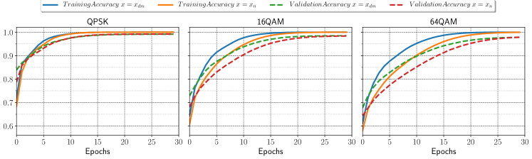
(a) Training and Validation Accuracies

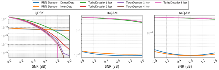
(b) BER Curves

Figure 6: Decoding Performance - Problem 3 & 4

The testing accuracies for both the turbo encoding and decoding operations are consistent with the validation accuracies and are outlined in Table II

TABLE II: Testing Accuracy - No Noise

Problem	Testing accuracy
Turbo Encoding	67%
Turbo Decoding - 1	100%

Figs. 5(a) and 5(b) show the effect of number of GRU units and the number of samples on training and validation accuracies respectively. It can be seen, that if the number of GRU units is less than 200, the model fails to converge for the selected number of epochs. Hence, the choice of having 800 units is a safe assumption. Similarly, the choice of using 3000 samples for training the model also seems safe given that there is some jitter in accuracy for the number of samples<2000.

V-B Turbo Decoding on Demodulated and Channel Output Data

For problems 3 and 4, the data from the demodulator and the channel are used respectively. Fig. 6(a) shows the evolution of training and validation accuracies with respect to the number of epochs for the three modulation schemes. It can be seen clearly that the model shows good training and validation performance on Quadrature Phase Shift Keying (QPSK) when compared to that of 16-Quadrature Amplitude Modulation (QAM) and 64-QAM. It can also be seen that the model performance is similar on both the demodulated and noise data which shows the ability of the model to understand the modulation structure thereby eliminating the need for demodulating the data beforehand. A careful look at the validation accuracies when using both the demodulated and noise data reveals, that the model fails to converge for the considered number of epochs.

Fig. 6(b) shows the BER performance of the model on both the datasets (calculated as $1-\text{Testing Accuracy}$) for each given SNR. It can be seen that the RNN model outperforms the conventional turbo decoder (for all decoding iterations) for low SNRs (<0.4 dB). However, at higher SNRs, the turbo decoder’s BER drops down exponentially while the drop is only linear for the RNN decoder.

VI Conclusions & Future Work

Driven by the demand for a paradigm shift in communication system design, ML is extensively studied by researchers to assess its applicability to wireless networks especially at the PHY layer. In this regard, this paper presents a DL approach for encoding and decoding of turbo codes (LTE variant) using auto-encoders based on RNNs. To this end, this paper presents an RNN architecture based on GRUs and compares its performance with the conventional turbo encoder/decoder. Simulation results show that the proposed RNN architecture is able to learn the structure of turbo codes and even outperform the conventional turbo decoder in terms of BER at lower SNRs. However, it lags behind the conventional turbo decoder at high SNRs by at least 2 orders of magnitude. A hybrid approach using RNN decoder at low SNRs and turbo decoder at high SNRs will be able to provide a performance enhancement in terms of decoding accuracy in the current wireless systems.

The current analysis considers a fixed data packet size of 64 bits. Without loss of generality, the proposed RNN architecture can be extended to support variable sized inputs and outputs. In this case, the problem needs to be reformulated as a sequence-to-sequence learning problem on the lines of natural language translation.

References

- [1] T. Wang, C.-K. Wen, H. Wang, F. Gao, T. Jiang, and S. Jin, “Deep Learning for Wireless Physical Layer: Opportunities and Challenges,” oct 2017.
- [2] I. Goodfellow, Y. Bengio, and A. Courville, Deep learning.
- [3] U. Challita, L. Dong, and W. Saad, “Proactive Resource Management in LTE-U Systems: A Deep Learning Perspective,” feb 2017.
- [4] R. Daniels, C. Caramanis, and R. Heath, “Adaptation in Convolutionally Coded MIMO-OFDM Wireless Systems Through Supervised Learning and SNR Ordering,” IEEE Transactions on Vehicular Technology, vol. 59, no. 1, pp. 114–126, jan 2010.
- [5] S. K. Pulliyakode and S. Kalyani, “Reinforcement learning techniques for Outer Loop Link Adaptation in 4G/5G systems,” aug 2017.
- [6] R. Sattiraju, J. Kochems, and H. D. Schotten, “Machine learning based obstacle detection for Automatic Train Pairing,” in 2017 IEEE 13th International Workshop on Factory Communication Systems (WFCS). IEEE, may 2017, pp. 1–4.
- [7] J. Vieira, E. Leitinger, M. Sarajlic, X. Li, and F. Tufvesson, “Deep Convolutional Neural Networks for Massive MIMO Fingerprint-Based Positioning,” aug 2017.
- [8] I. Ortuno, M. Ortuno, and J. Delgado, “Error correcting neural networks for channels with Gaussian noise,” in [Proceedings 1992] IJCNN International Joint Conference on Neural Networks, vol. 4. IEEE, 1992, pp. 295–300.
- [9] J. Bruck and M. Blaum, “Neural networks, error-correcting codes, and polynomials over the binary n-cube,” IEEE Transactions on Information Theory, vol. 35, no. 5, pp. 976–987, 1989.
- [10] A. Nandi and E. Azzouz, “Modulation recognition using artificial neural networks,” Signal Processing, vol. 56, no. 2, pp. 165–175, jan 1997.
- [11] T. O’Shea and J. Hoydis, “An Introduction to Deep Learning for the Physical Layer,” IEEE Transactions on Cognitive Communications and Networking, vol. 3, no. 4, pp. 563–575, dec 2017.
- [12] A. Weinand, M. Karrenbauer, J. Lianghai, and H. D. Schotten, “Physical Layer Authentication for Mission Critical Machine Type Communication using Gaussian Mixture Model based Clustering,” nov 2017.
- [13] C.-K. Wen, S. Jin, K.-K. Wong, J.-C. Chen, and P. Ting, “Channel Estimation for Massive MIMO Using Gaussian-Mixture Bayesian Learning,” IEEE Transactions on Wireless Communications, vol. 14, no. 3, pp. 1356–1368, mar 2015.
- [14] S. Chen, G. Gibson, C. Cowan, and P. Grant, “Adaptive equalization of finite non-linear channels using multilayer perceptrons,” Signal Processing, vol. 20, no. 2, pp. 107–119, jun 1990.
- [15] R. Annauth and H. Rughooputh, “Neural network decoding of turbo codes,” in IJCNN’99. International Joint Conference on Neural Networks. Proceedings (Cat. No.99CH36339), vol. 5. IEEE, pp. 3336–3341.
- [16] W. Caid and R. Means, “Neural network error correcting decoders for block and convolutional codes,” in [Proceedings] GLOBECOM ’90: IEEE Global Telecommunications Conference and Exhibition. IEEE, pp. 1028–1031.
- [17] A. Di Stefano, O. Mirabella, G. Di Cataldo, and G. Palumbo, “On the use of neural networks for Hamming coding,” in 1991., IEEE International Sympoisum on Circuits and Systems. IEEE, pp. 1601–1604.
- [18] H. Abdelbaki, E. Gelenbe, and S. El-Khamy, “Random neural network decoder for error correcting codes,” in IJCNN’99. International Joint Conference on Neural Networks. Proceedings (Cat. No.99CH36339), vol. 5. IEEE, pp. 3241–3245.
- [19] Xiao-An Wang and S. Wicker, “An artificial neural net Viterbi decoder,” IEEE Transactions on Communications, vol. 44, no. 2, pp. 165–171, 1996.
- [20] J. W. H. Kao, S. M. Berber, and A. Bigdeli, “A General Rate K / N Convolutional Decoder Based on Neural Networks with Stopping Criterion,” Advances in Artificial Intelligence, vol. 2009, pp. 1–11, jun 2009.
- [21] X. Wei, A. Yong, D. Z. I. J. Of, and U. 2016, “The Design and Implementation of Neural Network Encoding and Decoding.” International Journal of Simulation – Systems, Science & Technology, vol. 17, no. 38, pp. 17.1–17.5, 2016.
- [22] T. Gruber, S. Cammerer, J. Hoydis, and S. ten Brink, “On Deep Learning-Based Channel Decoding,” jan 2017.
- [23] TSGR, “TS 136 212 - V14.2.0 - LTE; Evolved Universal Terrestrial Radio Access (E-UTRA); Multiplexing and channel coding (3GPP TS 36.212 version 14.2.0 Release 14),” Tech. Rep., 2017.
- [24] K. Hornik, M. Stinchcombe, and H. White, “Multilayer feedforward networks are universal approximators,” Neural Networks, vol. 2, no. 5, pp. 359–366, jan 1989.
- [25] H. Siegelmann and E. Sontag, “On the Computational Power of Neural Nets,” Journal of Computer and System Sciences, vol. 50, no. 1, pp. 132–150, feb 1995.
- [26] C. Jiang, H. Zhang, Y. Ren, Z. Han, K.-C. Chen, and L. Hanzo, “Machine Learning Paradigms for Next-Generation Wireless Networks,” IEEE Wireless Communications, vol. 24, no. 2, pp. 98–105, apr 2017.
- [27] S. Hochreiter and J. Schmidhuber, “Long Short-Term Memory,” Neural Computation, vol. 9, no. 8, pp. 1735–1780, nov 1997.
- [28] K. Cho, B. van Merrienboer, C. Gulcehre, D. Bahdanau, F. Bougares, H. Schwenk, and Y. Bengio, “Learning Phrase Representations using RNN Encoder-Decoder for Statistical Machine Translation,” jun 2014.
- [29] D. P. Kingma and J. Ba, “Adam: A Method for Stochastic Optimization,” dec 2014.
- [30] H. Kim, Y. Jiang, R. Rana, S. Kannan, S. Oh, and P. Viswanath, “Communication Algorithms via Deep Learning,” may 2018.