Non-Hermitian boundary and interface states
in nonreciprocal higher-order topological metals and electrical circuits

Abstract

Non-Hermitian skin-edge states emerge only at one edge in one-dimensional nonreciprocal chains, where all states are localized at the edge irrespective of eigenvalues. The bulk topological number is the winding number associated with the complex energy spectrum, which is well defined for metals. We study non-Hermitian nonreciprocal systems in higher dimensions, and propose to realize them with the use of electric diode circuits. We first investigate one-dimensional interface states between two domains carrying different topological numbers, where all states are localized at the interface. They are a generalization of the skin-edge states. Then we generalize them into higher dimensions. We show that there emerge a rich variety of boundary states and interface states including surface, line and point states in three-dimensional systems. They emerge at boundaries of several domains carrying different topological numbers. The resulting systems are the first-order, second-order and third-order topological metals. Such states may well be observed by measuring the two-point impedance in diode circuits.

Introduction: The bulk-boundary correspondence has played an important role in topological systems. The emergence of boundary states is expected in all boundaries of a topological insulator (TI). For instance, when we consider a sufficiently long one-dimensional (1D) topological chain, edge states must emerge at both sides of the chain. Recently, non-Hermitian topological systems attract growing attentionBender ; Bender2 ; Kohmoto ; Scho ; Weimann ; Liang ; Pan ; Nori ; Zhu ; Konotop ; Fu ; UedaPRX ; Gana ; Katsura ; Yuce ; LangWang ; UedaHOTI ; EzawaLCR . In this context, a non-Hermitian bulk-edge correspondence was discovered in some 1D systems with the emergence of skin statesXiong ; Mart ; UedaPRX ; Kunst ; Yao ; Lee ; Jin ; Research ; SkinTop ; Luo . In particular, boundary states emerge only at one of the edges in a nonreciprocal 1D chain. One may wonder why the usual bulk-boundary correspondence is not valid. It is because the system is not an insulator but a non-Hermitian metal, though the topological charge is well defined to the bulkUedaPRX .

These non-Hermitian problems have been investigated by employing photonic systemsMark ; Scho ; Pan ; Weimann , microwave resonatorsPoli , wave guidesZeu , quantum walksRud ; Xiao , cavity systemsHoda and electric circuitsEzawaLCR ; Luo . In particular, it would be convenient to tune system parameters and to induce topological phase transitions in electric circuitsTECNature ; ComPhys ; Garcia ; Hel ; EzawaTEC ; EzawaLCR ; Luo .

On the other hand, the bulk-boundary correspondence has been generalized to include higher-order topological insulatorsPeng ; Lang ; Song ; Bena ; Schin ; EzawaKagome ; PhosHOTI . For three-dimensional (3D) crystals, the second-order TI has 1D hinge states but has no 2D surface states, while the third-order TI has 0D corner states but has neither surface nor hinge states. It is an intriguing problem how these higher-order topological states are generalized to nonreciprocal systems.

The aim of this paper is to explore the nonreciprocal bulk-boundary correspondence in higher dimensions. First of all, we are able to define non-Hermitian winding numbers in 2D square and 3D cubic systems, which are valid for gapless systems. Second, we obtain higher-order topological metals together with a rich variety of topological boundary and interface states. These states emerge together with characteristic peaks in the local density of states (LDOS). We also propose a method to detect such states by measuring two-point impedance in appropriately designed electric circuits.

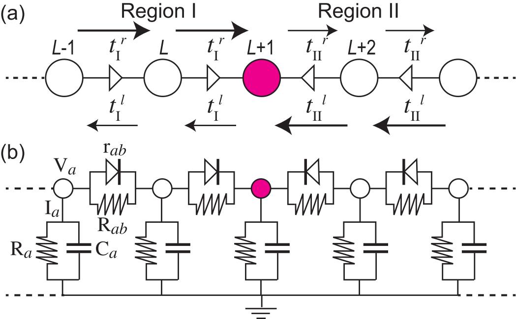
Figure 1: (a) Illustration of an interface in a 1D nonreciprocal system, where the amplitudes are different between the leftward ($t^{r}$) and rightward ($t^{l}$) hopping. We call the link rightward (denoted by $\rhd$) when $|t^{r}/t^{l}|>1$ and leftward (denoted by $\lhd$) when $|t^{l}/t^{r}|>1$. Links are oriented in this sense. The region made of the leftward (rightward) links has the topological number $w=+1$ ($-1$). There emerges a topological interface state at the junction ($\rhd,\lhd$) but not at ($\lhd,\rhd$). (b) Realization of a topological interface state by way of a diode circuit. The topological interface state is detected by observing a prominent impedance peak as in Fig.2(a3)–(c3).

Nonreciprocal system: We investigate a nonreciprocal system in $n$D hypercubic lattices [Fig.1(a)] described by

$$H=\sum_{a<b}(t_{ab}c_{b}^{\dagger}c_{a}+t_{ba}c_{a}^{\dagger}c_{b})+\sum_{a}U_{a}c_{a}^{\dagger}c_{a},$$ (1)

where $t_{ab}$ is the hopping amplitude between adjacent sites and $U_{a}$ is the on-site potential. Sites $a$ and $b$ are on the same axis in a hypercubic lattice, and the condition $a<b$ is well defined. The system is non-Hermitian for $\left|t_{ab}\right|\neq\left|t_{ba}\right|$. The potential $U_{a}$ can be complex. The 1D model is known as the Hatano-Nelson modelHatano ; UedaPRX . In the homogeneous system where $t_{ab}=t_{\mu}^{r}$, $t_{ba}=t_{\mu}^{l}$ for $a<b$ and $U_{a}=U$, the energy is given by

$$E\left(\boldsymbol{k}\right)=\sum_{\mu}(t_{\mu}^{r}e^{-ik_{\mu}}+t_{\mu}^{l}e^{ik_{\mu}})+U,$$ (2)

where $\mu=x$ for 1D, $\mu=x,y$ for 2D, and $\mu=x,y,z$ for 3D.

The energy is a complex number, which allows us to define a non-Hermitian winding number in $n$D as

$$w_{\mu}=\int_{-\pi}^{\pi}\frac{dk_{\mu}}{2\pi i}\partial_{k_{\mu}}\ln\left[E\left(\boldsymbol{k}\right)-\bar{E}_{\mu}\right],$$ (3)

where we have defined

$$\bar{E}_{\mu}=\int_{-\pi}^{\pi}\frac{dk_{\mu}}{2\pi}E\left(\boldsymbol{k}\right).$$ (4)

We note that $E\left(\boldsymbol{k}\right)-\bar{E}_{\mu}$ only depends on $k_{\mu}$ since $U_{\mu}$ gives a constant term with respect to $k_{\mu}$. It agrees with the previous definitionFu ; UedaPRX for 1D, where $w_{\mu}=1$ for $\left|t_{\mu}^{r}\right|<\left|t_{\mu}^{l}\right|$ and $w_{\mu}=-1$ for $\left|t_{\mu}^{r}\right|>\left|t_{\mu}^{l}\right|$. It is understood as the vorticity of the energyFu .

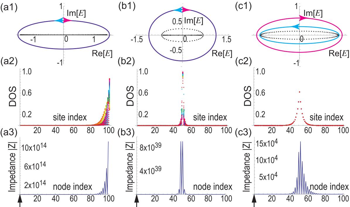
Figure 2: (a1)–(c1) Energy spectrum $E(k)$ in the complex plane, where $0\leq k\leq 2\pi$. The horizontal axis is Re[$E$] and the vertical axis is Im[$E$]. As $k$ increases from $k=0$, $E(k)$ draws a magenta (cyan) oval to form the bulk spectrum for the region I (II) and black dots to form the interface spectrum. A magenta (cyan) oval encircles the origin once clockwise (anticlockwise), yielding the topological number $w=-1(+1)$ to the region. Magenta and cyan ovals are degenerate in (a1) and (b1). (a2)–(c2) Plot of the LDOS for all eigenvalues, where different eigenvalues are indicated by different colors. All eigenvalues are degenerate in (c2). (a3)–(c3) Two-point impedance ($|Z|$ in unit of $\Omega$) where one node is fixed at the edge node indicated by an upward arrow. (a1)–(a3) for the edge state, where we set $t^{r}=1$, $t^{l}=1/2$. (b1)–(b3) for the interface state at the junction ($\rhd,\lhd$) as in Fig.1, where we set $t_{\text{l}}^{r}=t_{\text{lI}}^{l}=1$ and $t_{\text{l}}^{l}=t_{\text{lI}}^{r}=0.1$. (c1)–(c3) for a similar interface state, where $t_{\text{l}}^{r}=1$, $t_{\text{l}}^{l}=0.4$, $t_{\text{lI}}^{r}=0.5$ and $t_{\text{lI}}^{l}=0.8$.

The $n$D system is characterized by a set of $n$ winding numbers. There are two topological phases $w=\pm 1$ for 1D, there are four topological phases $(w_{x},w_{y})=(\pm 1,\pm 1)$ for 2D, and there are eight topological phases $(w_{x},w_{y},w_{z})=(\pm 1,\pm 1,\pm 1)$ for 3D. The system is always metallic since it is a one-band system. It is notable that the topological number is defined for metals, which is contrasted to the usual topological systems, where the topological number is defined for gapped systems such as topological insulators and superconductors. It is intriguing that we can define topological numbers for one-band systems in any dimensions.

The usual bulk-edge correspondence for topological insulators implies the emergence of the topological edges at both edges. Nevertheless, the bulk-edge correspondence for the present model is drastically different, which is allowed since the system is metallic: The topological edge states emerge only at the left (right) edge when $\ w=1$ ($w=-1$) for the 1D systemUedaPRX . A generalization to higher dimensional systems is a highly nontrivial problem, which we will explore in this paper.

Diode and nonreciprocal system: We propose a method to examine the results of the above nonreciprocal systems by realizing them with the use of electric circuits. Typical nonreciprocal devices are diodes. We thus consider a diode circuit as in Fig.1(b). The current $I$ is not proportional to the voltage $V$ for diodes, where the resistance has a dependence on $V$. However, we may in general approximate it by a linear resistance $r_{ab}$ for $a<b$. On the other hand, the resistance is perfect nonreciprocal, $r_{ba}=\infty$ for $a<b$. In this approximation, we obtain a linear nonreciprocal system with constant resistors.

The Kirchhoff’s current law for the circuit in Fig.1(b) is expressed as

$$I_{a}=C_{a}\frac{d}{dt}V_{a}+\frac{V_{a}}{R_{a}}+\sum_{b}\frac{V_{a}-V_{b}}{\bar{R}_{ab}},$$ (5)

where the sum over $b$ is taken for the two nearest neighbor nodes of $a$; $I_{a}$ is the current between node $a$ and the ground, $V_{a}$ is the voltage at node $a$, $R_{a}$ and $C_{a}$ are the resistance and the capacitance connected in parallel to the ground; finally, $\bar{R}_{ab}$ is the resistance between nodes $a$ and $b$,

$$\bar{R}_{ab}=\left\{\begin{array}[]{cc}r_{ab}R_{ab}/(r_{ab}+R_{ab})&\text{for\quad}a<b\\ R_{ab}&\text{for\quad}a>b\end{array}\right..$$ (6)

Here, we have added resistance $R_{ab}$ between two nodes $a$ and $b$ in parallel to the diode. The resistor $R_{ab}$ modifies the perfect nonreciprocity to imperfect nonreciprocity, while the resistor $R_{a}$ modifies the potential term, as we shall soon see below.

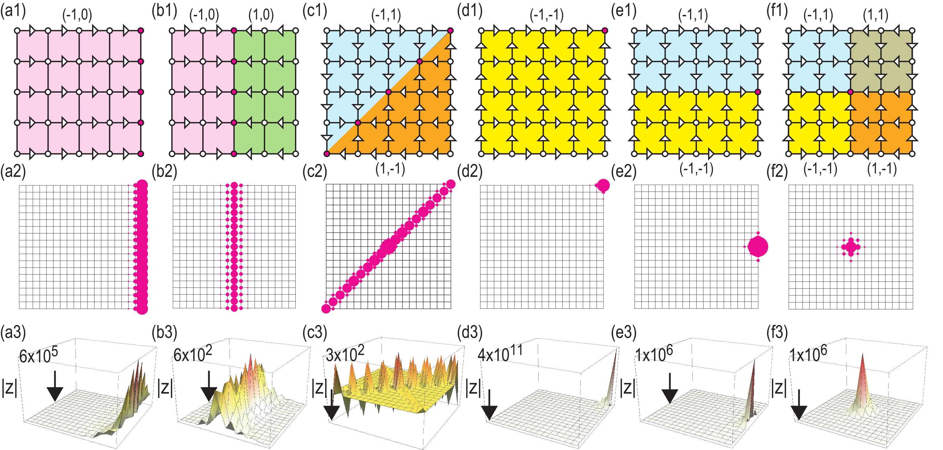
Figure 3: (a1)–(f1) Illustration of various topological boundary and interface states (marked in magenta) in 2D nonreciprocal systems. These states emerge at a boundary or an interface where the opposite nonreciprocities meet in such an order as indicated in the figures. They are (a) edge, (b) interface, (c) diagonal, (d) corner (e) edge-central and (f) bulk-central states. We obtain first-order topological metals (a,b,c), and second-order topological metals (d,e,f). Links are oriented in the same way as in the 1D nonreciprocal system (see Fig.1). Here in 2D, there are four orientations, rightward ($\rhd$), leftward ($\lhd$), upward ($\triangle$) and downward ($\triangledown$). A 2D region is indexed by a pair of topological charges ($w_{x},w_{y}$), where $w_{x}=\pm 1$ and $w_{y}=\pm 1$. (a2)–(f2) Sum of the LDOS of the eigen functions for all eigenvalues, which have large peaks at topological boundaries: The magnitude of a peak is represented by the size of a magenta disk. It is possible to interpret the lattice structures (a1)–(f1) as diode circuits as in Fig.1. (a3)–(f3) Two-point impedance ($|Z|$ in unit of $\Omega$), where one node is fixed as indicated by an arrow. A link is either oriented (nonreciprocal) or not (reciprocal). If not we have set $t_{ab}=1$. If oriented, we have set $t_{ab}=1$ for the positive orientation and $t_{ab}=1/4$ for the negative orientation.

The admittance matrix $J_{ab}\left(\omega\right)$ is defined byComPhys ; TECNature ; Hel ; Lu ; EzawaTEC ; EzawaLCR

$$I_{a}\left(\omega\right)=\sum_{b}J_{ab}\left(\omega\right)V_{b}\left(\omega\right),$$ (7)

with

$$J_{ab}\left(\omega\right)\equiv\left(-\sum_{b}\frac{1}{\bar{R}_{ab}}+\frac{1}{R_{a}}+i\omega C_{a}\right)\delta_{ab}+\frac{1}{\bar{R}_{ab}}.$$ (8)

There is a one-to-one correspondence between the admittance matrix $J_{ab}$ and the tight-binding Hamiltonian (1) with

$$t_{ab}=\frac{1}{\bar{R}_{ab}},\quad V_{a}=-\sum_{b}\frac{1}{\bar{R}_{ab}}+\frac{1}{R_{a}}+i\omega C_{a}.$$ (9)

We can set the real part of $V_{a}$ to be a constant by tuning $R_{a}$. The perfect nonreciprocal system with the forward-backward connection is realized by connecting perfect diodes so that the current flows right (left) going in the region I (II), as shown in Fig.1.

The local density of states of the eigenfunction of $J_{ab}$ is well observed by the two-point impedance, which is given byComPhys ; TECNature

$$Z_{ab}=\frac{V_{a}-V_{b}}{I_{ab}}=G_{aa}+G_{bb}-G_{ab}-G_{ba},$$ (10)

where $G$ is the Green function defined by the inverse of the admittance matrix $G_{ab}\equiv J_{ab}^{-1}$.

1D nonreciprocal system: We first study the Hatano-Nelson model in order to study interface states. We consider a closed chain with the length $2L$, where the hoppings are $t_{\text{I}}^{r}$ and $t_{\text{I}}^{l}$ for $1\leq n\leq L$ and $t_{\text{II}}^{r}$ and $t_{\text{II}}^{l}$ for $L+1\leq n\leq 2L$. We call the sites $1\leq n\leq L$ the region I and the sites $L+1\leq n\leq 2L$ the region II. Being a closed chain, it has two interfaces at the sites $n=L+1$ and $n=1$.

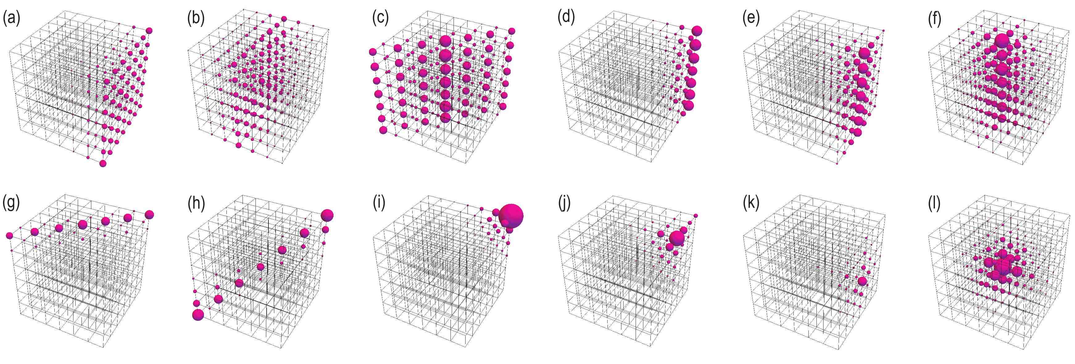
Figure 4: Illustration of various topological boundary and interface states and LDOS in 3D nonreciprocal systems. The magnitude of the LDOS peak is represented by the size of the magenta ball. These states emerge at a boundary or an interface where the opposite nonreciprocities meet in a certain order. LDOS representing (a) surface, (b) interface, (c) diagonal interface, (d) hinge, (e) surface-central line, (f) body-central line, (g) surface-diagonal line, (h) body-diagonal line and (i) corner, (j) hinge-central point, (k) surface-central point and (l) body-central point states. They are first-order topological metals (a,b,c), second-order topological metals (d,e,f,g,h), and third-order topological metals (i,j,k,l). A link is either oriented (nonreciprocal) or not (reciprocal). If not we have set $t_{ab}=1$. If oriented, we have set $t_{ab}=1$ for the positive orientation and $t_{ab}=1/4$ for the negative orientation.

In order to study non-Hermitian interface states, we diagonalized the Hamiltonian (1) in 1D. The eigen function is indexed by the site $n$ and labeled as $\left(\psi_{1},\psi_{2},\cdots\right)$. We may solve the eigenvalue problem exactly when the relation $t_{\text{I}}^{l}t_{\text{I}}^{r}=t_{\text{II}}^{l}t_{\text{II}}^{r}$ and $U_{a}=0$ hold. For $\left|t_{\text{II}}^{r}/t_{\text{I}}^{r}\right|<1$, the interface states emerge only at $n=L+1$ and are given bySupMat

$$\psi_{n} = \alpha^{L+1-n}\text{ for }n\leq L,$$ (11)

$$\psi_{n} = \beta^{n-L-1}\text{ for }n>L,$$ (12)

with $\alpha=\sqrt{t_{\text{II}}^{r}/t_{\text{I}}^{r}}e^{i\pi/L}$ and $\beta=\sqrt{t_{\text{II}}^{r}/t_{\text{I}}^{r}}e^{-i\pi/L}$. The eigenvalues are $E=\sqrt{t_{\text{I}}^{r}t_{\text{II}}^{r}}e^{i\pi/L}+\sqrt{t_{\text{I}}^{l}t_{\text{II}}^{l}}e^{-i\pi/L}$. All eigen functions are exponentially localized at the site $n=L+1$. All penetration depths are identical and given by $\xi=\frac{1}{2}\left|\ln\left(t_{\text{I}}^{r}/t_{\text{II}}^{r}\right)\right|$ between the regions I and II.

There is another exact solution. When $t_{\text{I}}^{r}\neq t_{\text{II}}^{l}$, $t_{\text{I}}^{r}\neq 0$, $t_{\text{II}}^{l}\neq 0$ and $t_{\text{I}}^{l}=t_{\text{II}}^{r}=0$ and $U_{n}=0$, all eigenvalues are zero and only the two eigen functions are nontrivial,

$$\psi_{n}^{\left(1\right)}\propto-t_{\text{II}}^{l}\delta_{n,L}+t_{\text{I}}^{r}\delta_{n,L+2},\qquad\psi_{n}^{\left(2\right)}=\delta_{n,L+1}.$$ (13)

The localization is strict and there is no penetration depth.

We may carry out numerical diagonalizations for any set of parameters. The bulk topological number is $w=-1$ in the region I and $w=1$ in the region II, which implies that the emergence of skin states at the right edge of the region I and the left edge of the region II. It is consistent with the fact that the interface states emerge at the site $n=L+1$ but there are no interface states at one site $n=1$. They are topological nonreciprocal interface states.

We show the energy spectrum and the LDOS in Fig.2. We have calculated the two-point impedance based on the formula (10) and show the results also in Fig.2. The characteristic behaviors of the LDOS are well signaled by measuring the two-point impedance, where one node is fixed at the site $n=1$ as in Fig.2(a3)–(c3).

2D square nonreciprocal system: We proceed to study the nonreciprocal Hamiltonian (1) in 2D. The simplest one is just to stack finite 1D chains, where the hopping along the $y$-axis is reciprocal. The bulk topological number is ($\pm 1,0$). Skin-edge states emerge along the $y$-axis as in Fig.3(a1). The next simplest one is to stack finite 1D chains with an interface. We obtain interface states along the $y$-axis at the junction of the two phases with ($-1,0$) and ($1,0$) in this order as in Fig.3(b1). It is also possible to have a diagonal interface state formed at the junction of the two phases with ($-1,-1$) and ($1,1$) in this order as in Fig.3(c1). These 1D objects are first-order topological boundary or interface states in 2D.

We may also have second-order topological boundary or interface states in 2D, which are 0D objects. Nonreciprocal corner states emerge at the right-up corner for the phase with ($-1,-1$) as in Fig.3(d1). Similarly, we have the right-down corner for the phase with ($-1,1$), the left-up corner for the phase with ($1,-1$) and the left-down corner for the phase with ($1,1$). Here we note a previous reportSkinTop showing the emergence of a corner state at the right-up corner without any bulk topological numbers. Furthermore, we obtain edge-central states at the corners of two phases with $\left(-1,1\right)$ and $\left(-1,-1\right)$, as showing Fig.3(e). Finally, we have bulk-central states at the corners of four phases with $\left(-1,1\right)$, $\left(1,1\right)$, $\left(-1,-1\right)$ and $\left(1,-1\right)$, as shown in Fig.3(f).

These boundary or interface states are manifested by evaluating the LDOS, whose results are shown in Fig.3(a2)–(f2). Experimental verifications would be carried out by designing diode circuits implied by Fig.3(a1)–(f1). We have calculated the two-point impedance based on the formula (10) by fixing one node as indicated by an arrow: See Fig.3(a3)–(f3). The behavior of the two-point impedance is not so simple as that of the LDOS, because it depends on the fixed point rather sensitively.

3D cubic nonreciprocal system: We also study the nonreciprocal Hamiltonian (1) in 3D. The simplest ones are just to stack 2D squares, where the hopping along the $z$-axis is reciprocal. For instance, we obtain 2D surface boundary or interface states Fig.4(a), (b) and (c) from Fig.3(a1), (b1) and (c1), respectively. They constitute the first-order topological metals. Similarly we obtain 1D line states Fig.4(d), (e) and (f) at a boundary or interface from Fig.4(d1), (e1) and (f1), respectively. We may have another types of 1D lines as in Fig.4(g), (h) when appropriate nonreciprocity is introduced into the $z$-axis. They constitute the second-order topological metals. Finally, we may make a full use of nonreciprocity to generate 0D point states as in Fig.4(i), (j), (k) and (l). The bulk of the corner state Fig.4(i) has the topological charge $\left(-1,-1,-1\right)$. The bulk-central point in Fig.4(l) emerges at the common corners of eight topological phases $\left(w_{x},w_{y},w_{z}\right)$ where $w_{x}=\pm 1$, $w_{y}=\pm 1$ and $w_{z}=\pm 1$. They constitute the third-order topological metals.

The author is very much grateful to N. Nagaosa for helpful discussions on the subject. This work is supported by the Grants-in-Aid for Scientific Research from MEXT KAKENHI (Grants No. JP17K05490, No. JP15H05854 and No. JP18H03676). This work is also supported by CREST, JST (JPMJCR16F1 and JPMJCR1874).

We derive eqs.(11) and (12) in the main text. We write the eigen function as $\left(\psi_{1},\psi_{2},\cdots,\psi_{n},\cdots\right)$ with the site index $n$. The eigen equation is given by

$$\left(\begin{array}[]{ccccccccc}-\varepsilon&t_{\text{I}}^{l}&0&\cdots&\cdots&\cdots&\cdots&0&t_{\text{II}}^{r}\\ t_{\text{I}}^{r}&-\varepsilon&t_{\text{I}}^{l}&0&\cdots&\cdots&\cdots&\cdots&0\\ \ddots&\ddots&\ddots&\ddots&\ddots&\ddots&\ddots&\ddots&\ddots\\ 0&\cdots&t_{\text{I}}^{r}&-\varepsilon&t_{\text{I}}^{l}&0&0&\cdots&0\\ 0&\cdots&0&t_{\text{I}}^{r}&-\varepsilon&t_{\text{II}}^{l}&0&\cdots&0\\ 0&\cdots&0&0&t_{\text{II}}^{r}&-\varepsilon&t_{\text{II}}^{l}&\cdots&0\\ \ddots&\ddots&\ddots&\ddots&\ddots&\ddots&\ddots&\ddots&\ddots\\ 0&\cdots&\cdots&\cdots&\cdots&0&t_{\text{II}}^{r}&-\varepsilon&t_{\text{II}}^{l}\\ t_{\text{II}}^{l}&0&\cdots&\cdots&\cdots&\cdots&0&t_{\text{II}}^{r}&-\varepsilon\end{array}\right)\left(\begin{array}[]{c}\psi_{1}\\ \psi_{2}\\ \cdots\\ \psi_{L}\\ \psi_{L+1}\\ \psi_{L+2}\\ \cdots\\ \psi_{2L-1}\\ \psi_{2L}\end{array}\right)=0.$$ (S1)

We assume exponentially decaying solutions,

$$\psi_{L+1-n}=\alpha^{n},\qquad\psi_{L+1+n}=\beta^{n}.$$ (S2)

The eigen equation is simplified as

$$t_{\text{I}}^{r}\alpha^{2}-\varepsilon\alpha+t_{\text{I}}^{l} = 0,$$ (S3)

$$t_{\text{I}}^{r}\alpha-\varepsilon+t_{2}^{l}\beta = 0,$$ (S4)

$$t_{\text{II}}^{r}-\varepsilon\beta+t_{\text{II}}^{l}\beta^{2} = 0.$$ (S5)

We solve eq.(S4) as

$$\varepsilon=t_{\text{I}}^{r}\alpha+t_{\text{II}}^{l}\beta.$$ (S6)

By inserting eq.(S6) to eqs. (S3) and (S5), we find

$$-t_{\text{II}}^{l}\alpha\beta+t_{\text{I}}^{l} = 0,$$ (S7)

$$t_{\text{II}}^{r}-t_{\text{I}}^{r}\alpha\beta = 0,$$ (S8)

which gives the relation

$$\alpha\beta=\frac{t_{\text{I}}^{l}}{t_{\text{II}}^{l}}=\frac{t_{\text{II}}^{r}}{t_{\text{I}}^{r}},$$ (S9)

or

$$t_{\text{I}}^{l}t_{\text{I}}^{r}=t_{\text{II}}^{l}t_{\text{II}}^{r},$$ (S10)

which is the condition given in the main text. Since the chain is closed, we also have the equations

$$t_{\text{II}}^{r}\psi_{2L}-\varepsilon\psi_{1}+t_{\text{I}}^{l}\psi_{2} = 0,$$ (S11)

$$t_{\text{II}}^{r}\psi_{2L-1}-\varepsilon\psi_{2L}+t_{\text{II}}^{l}\psi_{1} = 0.$$ (S12)

By inserting eq.(S2) into these, we obtain

$$t_{\text{II}}^{r}\beta^{L-1}-\varepsilon\alpha^{L}+t_{\text{I}}^{l}\alpha^{L-1} = 0,$$ (S13)

$$t_{\text{II}}^{r}\beta^{L-2}-\varepsilon\beta^{L-1}+t_{\text{II}}^{l}\alpha^{L} = 0.$$ (S14)

By using eq.(S6), we have

$$\frac{1}{\beta}=\alpha\frac{t_{\text{I}}^{r}}{t_{\text{II}}^{r}}.$$ (S15)

Finally, we obtain

$$\alpha=\sqrt{t_{\text{II}}^{r}/t_{\text{I}}^{r}}e^{i\pi/L},\qquad\beta=\sqrt{t_{\text{II}}^{r}/t_{\text{I}}^{r}}e^{-i\pi/L},$$ (S16)

with the eigenvalues

$$\varepsilon=\sqrt{t_{1}^{\text{r}}t_{2}^{\text{r}}}e^{i\pi/L}+\sqrt{t_{1}^{\text{l}}t_{2}^{\text{l}}}e^{-i\pi/L}.$$ (S17)

References

- (1) C. M. Bender and S. Boettcher, Phys. Rev. Lett. 80, 5243 (1998).
- (2) C. M. Bender, D. C. Brody, and H. F. Jones, Phys. Rev. Lett. 89, 270401 (2002).
- (3) K. Esaki, M. Sato, K. Hasebe, and M. Kohmoto, Phys. Rev. B 84, 205128 (2011).
- (4) H. Schomerus, Opt. Lett. 38, 1912 (2013).
- (5) S. Weimann, M. Kremer, Y. Plotnik, Y. Lumer, S.Nolte, K. G. Makris, M. Segev, M. C. Rechtsman, and A. Szameit, Nat. Mater. 16, 433 (2017).
- (6) S.-D. Liang and G.-Y. Huang, Phys. Rev. A 87, 012118 (2013).
- (7) M. Pan, H. Zhao, P. Miao, S. Longhi, and L. Feng, Nat. Commun. 9, 1308 (2018).
- (8) D. Leykam, K. Y. Bliokh, Chunli Huang, Y. D. Chong, and Franco Nori, Phys. Rev. Lett. 118, 040401 (2017).
- (9) B. Zhu, R. Lu and S. Chen, Phys. Rev. A 89, 062102 (2014).
- (10) V. V. Konotop, J. Yang, and D. A. Zezyulin, Rev. Mod. Phys. 88, 035002 (2016).
- (11) R. El-Ganainy, K. G. Makris, M. Khajavikhan, Z. H. Musslimani, S. Rotter and D. N. Christodoulides, Nat. Physics 14, 11 (2018).
- (12) K. Kawabata, Y. Ashida, H. Katsura, M. Ueda, Phys. Rev. B 98, 085116 (2018).
- (13) C. Yuce, Phys. Rev. A 97, 042118 (2018).
- (14) L.-J. Lang, Y. Wang, H. Wang, Y. D. Chong, Phys. Rev. B 98, 094307 (2018).
- (15) H. Shen, B. Zhen and L. Fu, Phys. Rev. Lett. 120, 146402 (2018)
- (16) Z. Gong, Y. Ashida, K. Kawabata, K. Takasan, S. Higashikawa and M. Ueda, Phys. Rev. X 8, 031079 (2018).
- (17) T. Liu, Y.-R. Zhang, Q. Ai, Z. Gong, K. Kawabata, M. Ueda, F. Nori, arXiv:1810.04067.
- (18) M. Ezawa, cond-mat/arXiv:1810.04527.
- (19) Y. Xiong, J. Physics Communications 2, 035043 (2018).
- (20) V. M. Martinez Alvarez, J. E. Barrios Vargas, and L. E. F. Foa Torres, Phys. Rev. B 97, 121401 (2018).
- (21) F. K. Kunst, E. Edvardsson, J. C. Budich and E. J. Bergholtz, Phys. Rev. Lett. 121, 026808 (2018).
- (22) S. Yao and Z. Wang, Phys. Rev. Lett. 121, 086803 (2018).
- (23) C. H. Lee, R. Thomale, cond-mat/arXiv:1809.02125.
- (24) L. Jin and Z. Song, Phys. Rev. B 99, 081103 (2019).
- (25) K. Luo, R. Yu, and H. Weng, Research 2018, ID 6793752
- (26) C. H. Lee, L. Li and J. Gong, cond-mat/arXiv:1810.11824.
- (27) K. Luo, J. Feng, Y. X. Zhao, and R. Yu, arXiv:1810.09231.
- (28) K. G. Makris, R. El-Ganainy, D. N. Christodoulides, and Z. H. Musslimani, Phys. Rev. Lett. 100, 103904 (2008).
- (29) C. Poli, M. Bellec, U. Kuhl, F. Mortessagne and H. Schomerus, Nat. Com. 6, 6710 (2015).
- (30) J. M. Zeuner, M. C. Rechtsman, Y. Plotnik, Y. Lumer, S. Nolte, M. S. Rudner, M. Segev, and A. Szameit, Phys. Rev. Lett. 115, 040402 (2015).
- (31) M. S. Rudner and L. S. Levitov, Phys. Rev. Lett. 102, 065703 (2009).
- (32) L. Xiao, X. Zhan, Z. H. Bian, K. K. Wang, X. Zhang, X. P. Wang, J. Li, K. Mochizuki, D. Kim, N. Kawakami, W. Yi, H. Obuse, B. C. Sanders, and P. Xue, Nat. Physics 13, 1117 (2017).
- (33) H. Hodaei, A. U Hassan, S. Wittek, H. Garcia-Gracia, R. El-Ganainy, D. N. Christodoulides and M. Khajavikhan, Nature 548, 187 (2017).
- (34) S. Imhof, C. Berger, F. Bayer, J. Brehm, L. Molenkamp, T. Kiessling, F. Schindler, C. H. Lee, M. Greiter, T. Neupert, R. Thomale, Nat. Phys. 14, 925 (2018).
- (35) C. H. Lee , S. Imhof, C. Berger, F. Bayer, J. Brehm, L. W. Molenkamp, T. Kiessling and R. Thomale, Communications Physics, 1, 39 (2018).
- (36) M. Serra-Garcia, R. Susstrunk and S. D. Huber, Phys. Rev. B 99, 020304(R) (2019).
- (37) T. Helbig, T. Hofmann, C. H. Lee, R. Thomale, S. Imhof, L. W. Molenkamp and T. Kiessling, cond-mat/arXiv:1807.09555.
- (38) M. Ezawa, Phys. Rev. B 98, 201402(R) (2018).
- (39) Y. Peng, Y. Bao, and F. von Oppen, Phys. Rev. B 95, 235143 (2017).
- (40) J. Langbehn, Y. Peng, L. Trifunovic, F. von Oppen, and P. W. Brouwer, Phys. Rev. Lett. 119, 246401 (2017).
- (41) Z. Song, Z. Fang, and C. Fang, Phys. Rev. Lett. 119, 246402 (2017).
- (42) W. A. Benalcazar, B. A. Bernevig, and T. L. Hughes, Phys. Rev. B 96, 245115 (2017).
- (43) F. Schindler, A. M. Cook, M. G. Vergniory, Z. Wang, S. S. P. Parkin, B. A. Bernevig, and T. Neupert, Science Advances 4, eaat0346 (2018).
- (44) M. Ezawa, Phys. Rev. Lett. 120, 026801 (2018).
- (45) M. Ezawa, Phys. Rev. B 98, 045125 (2018).
- (46) N. Hatano and D. R. Nelson, Phys. Rev. Lett. 77, 570 (1996): Phys. Rev. B 56, 8651 (1997): Phys. Rev. B 58, 8384 (1998).
- (47) Y. Lu, N. Jia, L. Su, C. Owens, G. Juzeliunas, D. I. Schuster and J. Simon, Phys. Rev. B 99, 020302(R) (2019).
- (48) See Supplemental Material at [URL] for the derivation of eqs.(11) and (12).
Supplemental Material