Bifurcation analysis of rotating axially compressed imperfect nano-rod

Abstract

Static stability problem for axially compressed rotating nano-rod clamped at one and free at the other end is analyzed by the use of bifurcation theory. It is obtained that the pitchfork bifurcation may be either super- or sub-critical. Considering the imperfections in rod’s shape and loading, it is proved that they constitute the two-parameter universal unfolding of the problem. Numerical analysis also revealed that for non-locality parameters having higher value than the critical one interaction curves have two branches, so that for a single critical value of angular velocity there exist two critical values of horizontal force.

Keywords: rotating nano-rod, critical load parameters, Lyapunov-Schmidt reduction, two-parameter universal unfolding.

1 Introduction and problem formulation

The problem of static stability of cantilevered rotating axially compressed rod displaying non-local effects is studied through the bifurcation theory, extending the results presented in [9], where the Euler method of adjacent equilibrium configuration is used to obtain critical values of the angular velocity and intensity of the horizontal axial force acting on the tip of rod’s free end. The obtained critical values are shown to represent the bifurcation points by using the Crandall-Rabinowitz theorem. Further, the Lyapunov-Schmidt reduction method is applied in order to obtain bifurcation equation corresponding to the non-linear equilibrium equations of rotating compressed rod and it is shown that the problem admits pitchfork bifurcation. Imperfections in shape, represented by the existence of a small initial deformation of the rod, and imperfections in loading, represented by the existence of a force of small intensity acting perpendicularly to rod’s axis on the tip of the rod, are also taken into account and it is proved that the selected imperfections constitute the universal unfolding of the problem. Moreover, the results presented in [9] are extended by finding the degenerate odd buckling modes for high values of non-locality parameter. Considering the non-locality effects, included through the stress gradient Eringen moment-curvature constitutive relation, the results of [4], where the same problem is analyzed in the case of Bernoulli-Euler constitutive equation, are extended as well.

The buckling problem of a rotating compressed rod, described by the elastic moment-curvature constitutive equation, is considered in [3, 10, 17, 20], while in [5, 7] the rod is allowed to have variable cross section and extensible axis, and in [19] there are additional rigid bodies attached to the rod. Static stability problem of a non-local rotating compressed rod, described by the Eringen stress gradient constitutive model, is studied in [8, 9] for the clamped-clamped and clamped-free rod, while in [1] a non-local clamped-free rod rotating about the axis perpendicular to rod’s axis is considered. The application of non-local theory in the static and dynamic stability problems of different types of rods is quite extensive, see the review articles [2, 13, 18] and book [12].

Consider a rectangular Cartesian coordinate system $xOy$ forming a plane $\Pi$ that rotates about the $x$-axis with the constant angular velocity $\omega.$ Placed in its undeformed state in plane $\Pi,$ an inextensible rod of length $L$ and initial curvature $R_{0},$ changing along the rod, is fixed in the origin of a coordinate system at one of its ends, while its other end is free. Being in the relative equilibrium in plane $\Pi,$ the rod rotates and under the influence of inertial force it may lose its stability and attain the relative equilibrium in the bent configuration, as shown in Figure 1.

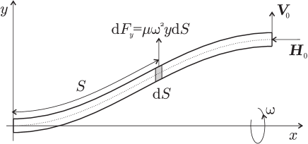
Figure 1: Rotating axially compressed imperfect nano-rod.

Differential equations and geometrical relations describing the relative equilibrium in plane $\Pi$ are:

$$H^{\prime}=0,\;\;\;\;V^{\prime}=-\mu\omega^{2}y,\;\;\;\;M^{\prime}=-V\cos\theta+H\sin\theta,$$ (1)

$$x^{\prime}=\cos\theta,\;\;\;\;y^{\prime}=\sin\theta,$$ (2)

see [6], where $H,$ $V,$ $M,$ $x,$ $y$ and $\theta$ are functions of rod’s arc length $S\in\left[0,L\right]$ and $\left(\cdot\right)^{\prime}=\frac{\mathrm{d}}{\mathrm{d}S}\left(\cdot\right),$ with $H$ and $V$ being components of the contact force in an arbitrary cross-section along $x$- and $y$-axis respectively, $M$ being the bending moment, $x$ and $y$ denoting the coordinates of an arbitrary point of a rod, and $\theta$ denoting the angle between the $x$-axis and tangent to rod’s axis, while the constant mass density per unit length of the rod is denoted by $\mu.$

The rod is assumed to display non-local effects and the moment-curvature constitutive equation is assumed in the form of the Eringen stress-gradient type model of non-locality as

$$M-\ell^{2}M^{\prime\prime}=EI\,\left(\frac{1}{R}-\frac{1}{R_{0}}\right),\;\;\text{with}\;\;\frac{1}{R}=\theta^{\prime}=\frac{y^{\prime\prime}}{\sqrt{1-\left(y^{\prime}\right)^{2}}},\text{ and }\frac{1}{R_{0}}=\frac{y_{0}^{\prime\prime}}{\sqrt{1-\left(y_{0}^{\prime}\right)^{2}}},$$ (3)

where $\frac{1}{R}$ and $\frac{1}{R_{0}}$ are the curvatures at equilibrium and initial configuration as functions of arc-length $S$, while the constants are: modulus of elasticity $E,$ moment of inertia of cross-section $I,$ and length-scale parameter $\ell.$ More on the Eringen type stress-gradient constitutive equations can be found in [14].

System of equations (1) - (3) is subject to boundary conditions

$$x\left(0\right)=0,\;\;y\left(0\right)=0,\;\;\theta(0)=0,\;\;H\left(L\right)=-H_{0},\;\;V\left(L\right)=V_{0},\;\;M\left(L\right)=0,$$ (4)

corresponding to the configuration shown in Figure 1. Note that (1)₁ and (4)₄ imply $H\left(S\right)=-H_{0}.$

Dimensionless variables and parameters

$$t=\frac{S}{L},\;\;\bar{x}=\frac{x}{L},\;\;\bar{y}=\frac{y}{L},\;\;\bar{R}=\frac{R}{L},\;\;\bar{R}_{0}=\frac{R_{0}}{L},\;\;v=\frac{VL^{2}}{EI},\;\;m=\frac{ML}{EI},\;\;\kappa=\left(\frac{\ell}{L}\right)^{2},$$

$$\lambda_{1}=\frac{\mu\omega^{2}L^{4}}{EI},\;\;\lambda_{2}=\frac{H_{0}L^{2}}{EI},\;\;\alpha_{1}=\frac{1}{\left\|R_{0}\right\|_{L^{\infty}\left[0,1\right]}},\;\;\alpha_{2}=\frac{V_{0}L^{2}}{EI},$$

where $\bar{R}_{0}\left(t\right)=\left\|\bar{R}_{0}\right\|_{L^{\infty}\left[0,1\right]}\rho_{0}\left(t\right),$ with $\left\|\bar{R}_{0}\right\|_{L^{\infty}\left[0,1\right]}=\sup_{t\in\left[0,1\right]}\left|\bar{R}_{0}\left(t\right)\right|$ and $\rho_{0}\left(t\right)=\frac{\bar{R}_{0}\left(t\right)}{\left\|\bar{R}_{0}\right\|_{L^{\infty}\left[0,1\right]}},$ after omitting bars, transform system of equations (1) - (3), subject to (4), into

$$\dot{v}=-\lambda_{1}y,\;\;\dot{m}=-v\cos\theta-\lambda_{2}\sin\theta,\;\;\dot{x}=\cos\theta,\;\;\dot{y}=\sin\theta,\;\;m-\kappa\ddot{m}=\dot{\theta}-\frac{\alpha_{1}}{\rho_{0}},$$ (5)

$$x(0)=0,\;\;y(0)=0,\;\;\theta(0)=0,\;\;v(1)=\alpha_{2},\;\;m(1)=0,$$ (6)

where $\left(\cdot\right)^{\cdot}=\frac{\mathrm{d}}{\mathrm{d}t}\left(\cdot\right)$ and $\dot{\theta}=\frac{\ddot{y}}{\sqrt{1-\dot{y}^{2}}}.$

Parameters $\lambda_{1}$ and $\lambda_{2},$ corresponding to the angular velocity and intensity of the horizontal force, are considered as load parameters, while parameters $\alpha_{1}$ and $\alpha_{2},$ corresponding to the maximal value of rod’s initial curvature and intensity of the vertical force, are considered as imperfections in shape and loading. It is obvious from the governing system of equations (5), subject to boundary conditions (6), that, for all real values of load parameters and zero values of imperfection parameters, it admits the trivial solution

$$x_{0}=S,\;\;y_{0}=0,\;\;\theta_{0}=0,\;\;v_{0}=0,\;\;m_{0}=0.$$

The critical values of load parameters $\lambda_{01}$ and $\lambda_{02}=\lambda_{02}\left(\lambda_{01}\right)$ are found in [9] using the Euler method of adjacent equilibrium configuration, i.e., by solving for the non-trivial solutions the linearized system of equations (5), subject to (6), with $\alpha_{1}=0$ and $\alpha_{2}=0.$ The present analysis will show that in the neighborhood of critical loading values there also exists the non-trivial solution to non-linear system of equations (5), subject to (6), bifurcating from the trivial solution at the critical loading value. The stability problem for perfect rod, i.e., initially straight rod without vertical force acting on its tip (zero values of imperfection parameters), will be studied in Section 2, while in Section 3 the study will focus on the stability problem for imperfect rod, i.e., rod having small initial deformation with vertical force of small intensity acting on its tip (non-zero values of imperfection parameters). Section 4 is devoted to numerical analysis of the interaction curve equation, mode shapes, bifurcation equation for perfect and imperfect rod.

2 Bifurcation points for perfect rod

The static stability problem is considered for the perfect rod, i.e., rotating rod without initial deformation, loaded by the horizontal axial force acting at its tip. The system of equations describing the equilibrium of perfect rod is (5), subject to boundary conditions (6), with $\alpha_{1}=\alpha_{2}=0$ and it reads

$$\dot{v}=-\lambda_{1}y,\;\;\dot{m}=-v\sqrt{1-\dot{y}^{2}}-\lambda_{2}\dot{y},\;\;m-\kappa\ddot{m}=\frac{\ddot{y}}{\sqrt{1-\dot{y}^{2}}},$$ (7)

$$y(0)=0,\;\;\dot{y}(0)=0,\;\;v(1)=0,\;\;m(1)=0.$$ (8)

System of equations (7), subject to (8), can be reduced to a single equation, represented by the action of a non-linear operator on deflection $y$ equated with zero. The operator is obtained either as the integro-differential operator of the second order, or as the differential operator of the fourth order. In both cases, (7)₂ is differentiated, (7)₁ is used, and such obtained expression is substituted into (7)₃ yielding

$$m=\left(1+\kappa v\dot{y}-\kappa\lambda_{2}\sqrt{1-\dot{y}^{2}}\right)\frac{\ddot{y}}{\sqrt{1-\dot{y}^{2}}}+\kappa\lambda_{1}y\sqrt{1-\dot{y}^{2}}.$$ (9)

The equation

$$M^{2}\left(\lambda,y\right)=0,\;\;\lambda\in\mathbb{R}^{2},\;y\in C^{k}\left(\left[0,1\right]\right),\text{ }k\geq 2,$$ (10)

with the operator $M^{2},$ defined by

$$M^{2}\left(\lambda,y\right):=\ddot{y}-\sqrt{1-\dot{y}^{2}}\frac{\lambda_{1}\left(J_{2}y-\kappa y\sqrt{1-\dot{y}^{2}}\right)+\lambda_{2}I_{1}\dot{y}}{1+\kappa\lambda_{1}\dot{y}\left(I_{1}y\right)-\kappa\lambda_{2}\sqrt{1-\dot{y}^{2}}},$$ (11)

where, for $z\in L^{1}\left[0,1\right],$

$$J_{2}z\left(t\right):=\int_{t}^{1}\int_{\tau}^{1}z(\eta)\sqrt{1-\dot{z}^{2}\left(\tau\right)}\mathrm{d}\eta\,\mathrm{d}\tau\;\;\text{and}\;\;I_{1}z\left(t\right):=\int_{t}^{1}z\left(\tau\right)\mathrm{d}\tau,$$

is obtained by integrating (7)₁ and (7)${}_{2},$ taking into account (8)₃ and (8)₄ and by substituting such obtained expressions into (9). Note that $M^{2}:\mathbb{R}^{2}\times C^{k}\left(\left[0,1\right]\right)\rightarrow C^{k-2}\left(\left[0,1\right]\right),$ $k\geq 2.$ The equation (10) is subject to boundary conditions (8)₁ and (8)${}_{2},$ i.e.,

$$BC^{2}=\left\{y:y\left(0\right)=0,\;\;\dot{y}\left(0\right)=0\right\}.$$ (12)

The equation

$$M^{4}\left(\lambda,y\right)=0,\;\;\lambda\in\mathbb{R}^{2},\;y\in C^{k}\left(\left[0,1\right]\right),\text{ }k\geq 4,$$ (13)

with the operator $M^{4},$ defined by

$$M^{4}\left(\lambda,y\right):=\left(\frac{\Big{(}\frac{\ddot{y}}{\sqrt{1-\dot{y}^{2}}}\Big{)}^{\boldsymbol{\cdot}}\left(1-\kappa\lambda_{2}\sqrt{1-\dot{y}^{2}}\right)+\kappa\lambda_{1}\dot{y}\left(\sqrt{1-\dot{y}^{2}}-\frac{2y\ddot{y}}{\sqrt{1-\dot{y}^{2}}}\right)+\lambda_{2}\dot{y}\left(1+\kappa\Big{(}\frac{\ddot{y}}{\sqrt{1-\dot{y}^{2}}}\Big{)}^{2}\right)}{\kappa\dot{y}\Big{(}\frac{\ddot{y}}{\sqrt{1-\dot{y}^{2}}}\Big{)}^{\boldsymbol{\cdot}}+\left(1+\kappa\Big{(}\frac{\ddot{y}}{\sqrt{1-\dot{y}^{2}}}\Big{)}^{2}\right)\sqrt{1-\dot{y}^{2}}}\right)^{\boldsymbol{\cdot}}-\lambda_{1}y,$$ (14)

is obtained directly from (7)${}_{1},$ since the term in brackets is $v,$ obtained by differentiating (9), with the subsequent use of (7)${}_{2}.$ Note $M^{4}:\mathbb{R}^{2}\times C^{k}\left(\left[0,1\right]\right)\rightarrow C^{k-4}\left(\left[0,1\right]\right),$ $k\geq 4.$ The equation (13) is subject to boundary conditions

$$BC^{4} = \Bigg{\{}y:y\left(0\right)=0,\;\;\dot{y}\left(0\right)=0,$$ (18)

$$\left(1-\kappa\lambda_{2}\sqrt{1-\dot{y}^{2}\left(1\right)}\right)\frac{\ddot{y}\left(1\right)}{\sqrt{1-\dot{y}^{2}\left(1\right)}}+\kappa\lambda_{1}y(1)\sqrt{1-\dot{y}^{2}\left(1\right)}\begin{tabular}[]{l}=\end{tabular}0,$$

$$\left(1-\kappa\lambda_{2}\sqrt{1-\dot{y}^{2}\left(1\right)}\right)\left.\left(\frac{\ddot{y}\left(t\right)}{\sqrt{1-\dot{y}^{2}\left(t\right)}}\right)^{\boldsymbol{\cdot}}\right|_{t=1}$$

$$+\left(\kappa\lambda_{1}\left(\sqrt{1-\dot{y}^{2}\left(1\right)}-2y\left(1\right)\frac{\ddot{y}\left(1\right)}{\sqrt{1-\dot{y}^{2}\left(1\right)}}\right)+\lambda_{2}\left(1+\kappa\left(\frac{\ddot{y}\left(1\right)}{\sqrt{1-\dot{y}^{2}\left(1\right)}}\right)^{2}\right)\right)\dot{y}(1)\begin{tabular}[]{l}=\end{tabular}0\Bigg{\}},$$

where the first two boundary conditions are (8)₁ and (8)${}_{2},$ while the third boundary condition is (8)${}_{4},$ with (9) calculated at $t=1$ and the fourth boundary condition is (8)${}_{3},$ with the nominator of the term in brackets in (14) calculated at $t=1.$

Equations (10), subject to (12), and (13), subject to (18), are equivalent. The focus is on finding bifurcation points to problem (10), (12) (or equivalently to (13), (18)). It is easy to verify that for all $\lambda\in\mathbb{R}^{2}$ there is a solution curve of (10), (12) (and of (13), (18)), through $\left(\lambda,0\right)$ and the critical value $\lambda_{0}$ for which there are other solution curves in neighborhood $U\times V\subset\mathbb{R}^{2}\times C^{k}\left(\left[0,1\right]\right),$ $k\geq 2,$ of $\left(\lambda_{0},0\right)$ for problem (10), (12) (or in neighborhood $U\times V\subset\mathbb{R}^{2}\times C^{k}\left(\left[0,1\right]\right),$ $k\geq 4,$ of $\left(\lambda_{0},0\right)$ for problem (13), (18)) are sought for. A necessary condition for $\lambda_{0}$ to be critical value is the failure of implicit function theorem, see e.g. [16, Theorem I.1.1], i.e., that

$$D_{y}M^{j}\left(\lambda_{0},0\right):C^{k}\left(\left[0,1\right]\right)\mapsto C^{k-j}\left(\left[0,1\right]\right)\;\text{is not bijective,}$$ (19)

with $j\in\left\{2,4\right\}$ and $k\geq 2$ for $j=2$ and $k\geq 4$ for $j=4,$ where $D_{y}$ denotes the Fréchet derivative. The Fréchet derivatives of $M^{2}$, $M^{4}$ and $BC^{4}$ at $\left(\lambda,0\right)$ are calculated as

$$\!\!\!\!\!\!\!\!\!\!\!\!\!\!\!\!\!\!L^{2}\left(\lambda\right)y\!\!\begin{tabular}[]{l}:=\end{tabular}\!\!D_{y}M^{2}\left(\lambda,0\right)y\begin{tabular}[]{l}=\end{tabular}\ddot{y}-\frac{\lambda_{1}}{1-\kappa\lambda_{2}}\left(I_{2}y-\kappa y\right)-\frac{\lambda_{2}}{1-\kappa\lambda_{2}}I_{1}\dot{y}$$ (22)

$$\!\!\!\!\!\!\!\!\!\!\!\!\!\!\!\!\!\!L^{4}\left(\lambda\right)y\!\!\begin{tabular}[]{l}:=\end{tabular}\!\!D_{y}M^{4}\left(\lambda,0\right)y\begin{tabular}[]{l}=\end{tabular}y^{\mathrm{IV}}(t)+\frac{\kappa\lambda_{1}+\lambda_{2}}{1-\kappa\lambda_{2}}\ddot{y}\left(t\right)-\frac{\lambda_{1}}{1-\kappa\lambda_{2}}y(t),$$ (25)

$$\!\!\!\!\!\!\!\!\!\!\!\!\!\!\!\!\!\!LBC\!\!\begin{tabular}[]{l}=\end{tabular}\!\!\left\{y\left(0\right)=0,\;\dot{y}\left(0\right)=0,\;\ddot{y}\left(1\right)\left(1-\kappa\lambda_{2}\right)+\kappa\lambda_{1}y(1)=0,\;y^{\mathrm{III}}\left(1\right)\left(1-\kappa\lambda_{2}\right)+\left(\kappa\lambda_{1}+\lambda_{2}\right)\dot{y}(1)=0\right\},$$ (27)

where

$$I_{2}z\left(t\right):=\int_{t}^{1}\int_{\tau}^{1}z\left(\eta\right)\mathrm{d}\eta\mathrm{d}\tau.$$

Finding $\lambda_{0}$ such that (19) holds is equivalent to finding $\lambda_{0}$ for which kernel of the operator $L^{2}\left(\lambda_{0}\right)$ (or $L^{4}\left(\lambda_{0}\right)$) is nontrivial (do not consists of $y=0$ only). For fixed $\lambda$, one finds kernel of the operator $L^{2}\left(\lambda\right)$ (or $L^{4}\left(\lambda\right)$) by solving the equation

$$L^{j}\left(\lambda\right)y=0,\;\;y\in Y^{j},\;j\in\left\{2,4\right\},$$ (28)

where

$$Y^{2}=\left\{y:y\in C^{k}\left(\left[0,1\right]\right),\;k\geq 2\right\}\cap BC^{2}\;\;\text{and}\;\;Y^{4}=\left\{y:y\in C^{k}\left(\left[0,1\right]\right),\;k\geq 4\right\}\cap LBC,$$

where $BC^{2}$ and $LBC$ are given by (12) and (27). Note that $Y^{2}$ and $Y^{4}$ are Hilbert spaces with usual scalar product $\left\langle y,q\right\rangle=\int_{0}^{1}y\left(t\right)q\left(t\right)\mathrm{d}t.$

The problems (28) for $j=2$ and (28) for $j=4$ are equivalent. Indeed, $\frac{\mathrm{d}^{2}}{\mathrm{d}t^{2}}\left(L^{2}\left(\lambda\right)y\right)=L^{4}\left(\lambda\right)y,$ with boundary conditions (27) obtained for $L^{2}\left(\lambda\right)y\left(1\right)=0$ and $\left.\frac{\mathrm{d}}{\mathrm{d}t}\left(L^{2}\left(\lambda\right)y\left(t\right)\right)\right|_{t=1}=0,$ while $I_{2}\left(L^{4}\left(\lambda\right)y\right)=L^{2}\left(\lambda\right)y$ is obtained by integration of (25) and use of the boundary conditions (27).

The problem (28) for $j=4$ is considered in [9]. The critical value $\lambda_{0}=\left(\text{$\lambda_{01},\lambda_{02}$}\right)$ is obtained from the condition of existence of nontrivial solution $y$ to problem (28), $j=4$, which requires that the determinant arising from boundary conditions (27) is equal to zero, i.e., as a solution of

$$f\left(\text{$\lambda_{1},\lambda_{2}$}\right)=\sqrt{\frac{\text{$\lambda_{1}$}}{1-\kappa\text{$\lambda_{2}$}}}\Bigg{(}2\text{$\lambda_{1}$}+\kappa\text{$\lambda_{1}$}\left(\kappa\text{$\lambda_{1}$}-\text{$\lambda_{2}$}\right)+\left(2\text{$\lambda_{1}$}+\text{$\lambda_{2}^{2}$}-\kappa\text{$\lambda_{1}\lambda_{2}$}\right)\cos\left(r_{1}\left(\text{$\lambda_{1},\lambda_{2}$}\right)\right)\,\cosh\left(r_{2}\left(\text{$\lambda_{1},\lambda_{2}$}\right)\right)$$

$$\qquad\qquad\qquad\qquad-\sqrt{\frac{\text{$\lambda_{1}$}}{1-\kappa\text{$\lambda_{2}$}}}\left(\text{$\lambda_{2}$}-\kappa\left(\text{$\lambda_{1}$}-\kappa\text{$\lambda_{1}\lambda_{2}$}+\text{$\lambda_{2}^{2}$}\right)\right)\sin\left(r_{1}\left(\text{$\lambda_{1},\lambda_{2}$}\right)\right)\,\sinh\left(r_{2}\left(\text{$\lambda_{1},\lambda_{2}$}\right)\right)\Bigg{)}=0,$$ (29)

where

$$r_{1}\left(\text{$\lambda_{1},\lambda_{2}$}\right) = \sqrt{\sqrt{\frac{\lambda_{1}}{1-\kappa\lambda_{2}}+\left(\frac{1}{2}\frac{\kappa\lambda_{1}+\lambda_{2}}{1-\kappa\lambda_{2}}\right)^{2}}+\frac{1}{2}\frac{\kappa\lambda_{1}+\lambda_{2}}{1-\kappa\lambda_{2}}},$$ (30)

$$r_{2}\left(\text{$\lambda_{1},\lambda_{2}$}\right) = \sqrt{\sqrt{\frac{\lambda_{1}}{1-\kappa\lambda_{2}}+\left(\frac{1}{2}\frac{\kappa\lambda_{1}+\lambda_{2}}{1-\kappa\lambda_{2}}\right)^{2}}-\frac{1}{2}\frac{\kappa\lambda_{1}+\lambda_{2}}{1-\kappa\lambda_{2}}}.$$ (31)

By the implicit function theorem, since $f\left(\text{$\lambda_{01},\lambda_{02}$}\right)=0$ and $\left.\frac{\partial f\left(\text{$\lambda_{1},\lambda_{2}$}\right)}{\partial\lambda_{2}}\right|_{\left(\text{$\lambda_{1},\lambda_{2}$}\right)=\left(\lambda_{01},\lambda_{02}\right)}\neq 0,$ in the neighborhood of $\lambda_{01},\lambda_{02},$ i.e., for $\lambda_{1}=\lambda_{01}+\Delta\lambda_{1}$ and $\lambda_{2}=\lambda_{02}+\Delta\lambda_{2},$ equation (29) is solved with respect to $\lambda_{2},$ i.e., there exists a unique differentiable function $\eta,$ such that $\lambda_{2}=\eta\left(\text{$\lambda_{1}$}\right)$ and

$$f\left(\text{$\lambda_{1},$}\eta\left(\text{$\lambda_{1}$}\right)\right)=0\;\;\text{and}\;\;\eta^{\prime}\left(\text{$\lambda_{1}$}\right)=\frac{\mathrm{d}\eta\left(\text{$\lambda_{1}$}\right)}{\mathrm{d}\text{$\lambda_{1}$}}=-\left.\frac{\frac{\partial f\left(\text{$\lambda_{1},\lambda_{2}$}\right)}{\partial\lambda_{1}}}{\frac{\partial f\left(\text{$\lambda_{1},\lambda_{2}$}\right)}{\partial\lambda_{2}}}\right|_{\left(\text{$\lambda_{1},\lambda_{2}$}\right)=\left(\text{$\lambda_{1},$}\eta\left(\text{$\lambda_{1}$}\right)\right)}.$$ (32)

Then also

$$\Delta\lambda_{2}=\eta^{\prime}\left(\text{$\lambda_{01}$}\right)\Delta\lambda_{1}.$$ (33)

Nontrivial solution to (28), $j=4$, corresponding to $\lambda_{0}=\left(\lambda_{01},\lambda_{02}\right)$ reads:

$$y_{l}\left(t\right)=C\left(\cos\left(r_{01}t\right)-\cosh\left(r_{02}t\right)-D\left(r_{01},r_{02}\right)\left(\sin\left(r_{01}t\right)-\frac{r_{01}}{r_{02}}\sinh\left(r_{02}t\right)\right)\right),$$ (34)

where $C$ is an arbitrary constant and $D$ is a constant given by

$$D\left(r_{01},r_{02}\right)=\frac{r_{01}^{2}\cos r_{01}+r_{02}^{2}\cosh r_{02}+\frac{\kappa\text{$\lambda_{01}$}}{1-\kappa\text{$\lambda_{02}$}}\left(\cosh r_{02}-\cos r_{01}\right)}{r_{01}^{2}\sin r_{01}+r_{01}r_{02}\sinh r_{02}+\frac{\kappa\text{$\lambda_{01}$}}{1-\kappa\text{$\lambda_{02}$}}\left(\frac{r_{01}}{r_{02}}\sinh r_{02}-\sin r_{01}\right)},$$

where parameters $r_{01}$ and $r_{02}$ are calculated from (30) and (31) for $\lambda_{0}$.

The kernel of operator $L^{j}\left(\lambda_{0}\right),$ $j\in\left\{2,4\right\},$ is one-dimensional space, i.e.,

$$\dim N\left(L^{j}\left(\lambda_{0}\right)\right)=1,\;\;j\in\left\{2,4\right\},$$ (35)

since $N\left(L^{j}\left(\lambda_{0}\right)\right)=\mathop{\mathrm{s}pan}[y_{L}]=\{ay_{L};\,a\in\mathbb{R}\},$ $j\in\left\{2,4\right\},$ where the normalized solution (34) is denoted by $y_{L}$, i.e. the solution with constant $C$ chosen such that $\left\|y_{L}\right\|_{Y^{j}}=1.$

Orthogonal complement of the range of $L^{j}\left(\lambda_{0}\right)$ is a kernel of the formal adjoint $L^{j\ast}\left(\lambda_{0}\right)$ of operator $L^{j}\left(\lambda_{0}\right)$, where the formal adjoint of an operator $L^{j}:Y^{j}\rightarrow Z^{j}$ is defined as an operator $L^{j\ast}:Z^{j}\rightarrow Y^{j},$ such that for all $y\in Y^{j}$ and all $q\in Z^{j}$ equality $\langle L^{j\ast}q,y\rangle_{Y^{j}}=\langle L^{j}y,q\rangle_{Z^{j}}$ holds, where $Z^{j}=C^{k-j}\left(\left[0,1\right]\right),$ $j\in\left\{2,4\right\}.$ Straightforward calculation gives

$$L^{2\ast}\left(\lambda\right)q\begin{tabular}[]{l}=\end{tabular}\ddot{y}-\frac{\lambda_{01}}{1-\kappa\lambda_{02}}\left(I_{2}y-\kappa y\right)-\frac{\lambda_{02}}{1-\kappa\lambda_{02}}I_{1}\dot{y},$$

$$LBC^{2\ast}\begin{tabular}[]{l}=\end{tabular}\bigg{\{}q(1)=0,\;\;\dot{q}(1)+\frac{\lambda_{02}}{1-\kappa\lambda_{02}}\left\langle 1,q\right\rangle=0,\;\;\ddot{q}\left(1\right)+\frac{\lambda_{01}}{1-\kappa\lambda_{02}}\left(\left\langle t,q\right\rangle-\left\langle 1,q\right\rangle\right)=0$$

$$\qquad\qquad\qquad q^{\mathrm{III}}\left(1\right)+\frac{\kappa\lambda_{01}+\lambda_{02}}{1-\kappa\lambda_{02}}\dot{q}(1)-\frac{\lambda_{01}}{1-\kappa\lambda_{02}}\left\langle 1,q\right\rangle=0\bigg{\}},$$

$$L^{4\ast}\left(\lambda\right)q\begin{tabular}[]{l}=\end{tabular}q^{\mathrm{IV}}(t)+\frac{\kappa\lambda_{01}+\lambda_{02}}{1-\kappa\lambda_{02}}\ddot{q}\left(t\right)-\frac{\lambda_{01}}{1-\kappa\lambda_{02}}q(t),$$

$$LBC^{4\ast}\begin{tabular}[]{l}=\end{tabular}\left\{q(0)=0,\;\;\dot{q}(0)=0,\;\;\ddot{q}\left(1\right)=0,\;\;q^{\mathrm{III}}\left(1\right)+\frac{\lambda_{02}}{1-\kappa\lambda_{02}}\dot{q}(1)=0\right\}.$$

The kernel of operator $L^{j\ast}\left(\lambda_{0}\right)$ is found by solving equation $L^{j\ast}\left(\lambda_{0}\right)q=0$, $q\in Z^{j},$ whose solution reads

$$q_{l}^{\left(2\right)}\left(t\right) = C\left(\cos\left(r_{01}t\right)+\frac{r_{02}^{2}}{r_{01}^{2}}\cosh\left(r_{02}t\right)-\frac{\cos r_{01}+\frac{r_{02}^{2}}{r_{01}^{2}}\cosh r_{02}}{\sin r_{01}+\frac{r_{02}}{r_{01}}\sinh r_{02}}\left(\sin\left(r_{01}t\right)+\frac{r_{02}}{r_{01}}\sinh(r_{02}t)\right)\right),$$ (40)

$$q_{l}^{\left(4\right)}\left(t\right) = C\left(\cos\left(r_{01}t\right)-\cosh\left(r_{02}t\right)-\frac{\cos r_{01}+\frac{r_{02}^{2}}{r_{01}^{2}}\cosh r_{02}}{\sin r_{01}+\frac{r_{02}}{r_{01}}\sinh r_{02}}\left(\sin\left(r_{01}t\right)-\frac{r_{01}}{r_{02}}\sinh(r_{02}t)\right)\right).$$ (41)

Therefore, the kernel of operator $L^{j\ast}\left(\lambda_{0}\right)$ is one-dimensional and

$$\mathop{\mathrm{c}odim}R(L^{j}\left(\lambda_{0}\right))=1,\;\;j\in\left\{2,4\right\}.$$ (42)

If $\lambda_{0}=\left(\lambda_{01},\eta\left(\lambda_{01}\right)\right)$ is critical value, then by Krasnoselskii theorem, $\left(\lambda_{0},0\right)$ is a bifurcation point of the nonlinear operators $M^{2}$ and $M^{4},$ since, according to (35), $\dim N\left(L^{j}\left(\lambda_{0}\right)\right)=1$ and it is of odd algebraic multiplicity. Although $\left(\lambda_{0},0\right)$ is proved to be a bifurcation point, the existence of nontrivial solution to (13) is also established by the use of Crandall-Rabinowitz theorem, see [16, Theorem I.5.1].

Theorem 1

Let $Y^{4}$ and $Z^{4}$ be defined as above and let operator $M^{4}$ be given by (14). Let $\lambda_{0}=\left(\lambda_{01},\eta\left(\lambda_{01}\right)\right)$ be the critical value for which there exists nontrivial solution to (28). Then $\left(\lambda_{0},0\right)=\left(\lambda_{01},\eta\left(\lambda_{01}\right),0\right)$ is a bifurcation point to (13).

Proof. Let $U$ and $V$ be open neighborhoods in $\mathbb{R}$ and $Y^{4}$ such that $\lambda_{01}\in U\subset\mathbb{R}$ and $0\in V\subset Y^{4}.$ Let $\bar{M}^{4}$ be operator on $\mathbb{R}\times Y^{4}$ defined as

$$\bar{M}^{4}\left(\lambda_{1},y\right):=M^{4}\left(\lambda_{1},\eta\left(\lambda_{1}\right),y\right).$$

Note that $\bar{M}^{4}\in C^{2}\left(U\times V,Z^{4}\right)$ and that $\bar{M}^{4}\left(\lambda_{1},0\right)=0\;$for all $\lambda_{1}\in\mathbb{R}.$ According to (35) and (42), the operator $\bar{M}^{4}\left(\lambda_{01},\cdot\right)$ is Fredholm operator of index zero. Further, by showing that $D_{y,\lambda_{1}}^{2}\bar{M}^{4}\left(\lambda_{01},0\right)y_{L}$ belongs to $N(L^{4\ast}\left(\lambda_{0}\right)),$ it will be proved that the requirement Crandall-Rabinowitz theorem [16, Theorem I.5.1] $D_{y,\lambda_{1}}^{2}\bar{M}^{4}\left(\lambda_{01},0\right)y_{L}\notin R\left(D_{y}\bar{M}^{4}\left(\lambda_{01},0\right)\right)$ is satisfied. Indeed,

$$D_{y,\lambda_{1}}^{2}\bar{M}^{4}\left(\lambda_{01},0\right)y_{L}=\left(\kappa\Lambda_{1}+\Lambda_{2}\right)\ddot{y}_{L}\left(t\right)-\Lambda_{1}y_{L}(t),$$

where

$$\Lambda_{1}=\frac{\kappa\lambda_{01}\eta^{\prime}\left(\lambda_{01}\right)-\kappa\eta\left(\lambda_{01}\right)+1}{\left(1-\kappa\eta\left(\lambda_{01}\right)\right)^{2}},\;\text{\ }\Lambda_{2}=\frac{\eta^{\prime}\left(\lambda_{01}\right)}{\left(1-\kappa\eta\left(\lambda_{01}\right)\right)^{2}},$$

so that

$$L^{4\ast}\left(\lambda_{0}\right) D_{y,\lambda_{1}}^{2}\bar{M}^{4}\left(\lambda_{01},0\right)y_{L}=L^{4\ast}\left(\lambda_{0}\right)\Big{(}\left(\kappa\Lambda_{1}+\Lambda_{2}\right)\ddot{y}_{L}\left(t\right)-\Lambda_{1}y_{L}(t)\Big{)}$$

$$=\Big{(}\left(\kappa\Lambda_{1}+\Lambda_{2}\right)\ddot{y}_{L}\left(t\right)-\Lambda_{1}y_{L}(t)\Big{)}^{\mathrm{IV}}+\frac{\kappa\lambda_{01}+\eta\left(\lambda_{01}\right)}{1-\kappa\eta\left(\lambda_{01}\right)}\Big{(}\left(\kappa\Lambda_{1}+\Lambda_{2}\right)\ddot{y}_{L}\left(t\right)-\Lambda_{1}y_{L}\left(t\right)\Big{)}^{\boldsymbol{\cdot}\boldsymbol{\cdot}}$$

$$\qquad-\frac{\lambda_{01}}{1-\kappa\eta\left(\lambda_{01}\right)}\Big{(}\left(\kappa\Lambda_{1}+\Lambda_{2}\right)\ddot{y}_{L}\left(t\right)-\Lambda_{1}y_{L}(t)\Big{)}$$

$$=\left(\kappa\Lambda_{1}+\Lambda_{2}\right)\left(y_{L}^{\mathrm{IV}}(t)+\frac{\kappa\lambda_{01}+\eta\left(\lambda_{01}\right)}{1-\kappa\eta\left(\lambda_{01}\right)}\ddot{y}_{L}\left(t\right)-\frac{\lambda_{01}}{1-\kappa\eta\left(\lambda_{01}\right)}y_{L}(t)\right)^{\boldsymbol{\cdot}\boldsymbol{\cdot}}$$

$$\qquad-\Lambda_{1}\left(y_{L}^{\mathrm{IV}}(t)+\frac{\kappa\lambda_{01}+\eta\left(\lambda_{01}\right)}{1-\kappa\eta\left(\lambda_{01}\right)}\ddot{y}_{L}\left(t\right)-\frac{\lambda_{01}}{1-\kappa\eta\left(\lambda_{01}\right)}y_{L}(t)\right)\begin{tabular}[]{l}=\end{tabular}0.$$

Thus, $\left(\lambda_{0},0\right)$ is the bifurcation point.   

In order to determine the type of bifurcation at point $\left(\lambda_{0},0\right),$ the reduction method of Lyapunov-Schmidt will be used. Let $Y^{2}$ and $Z^{2}$ be defined as above and let operator $M^{2}$ be given by (11). Consider mapping $M^{2}:U\times V\rightarrow Z^{2}$, with $U$ and $V$ being open neighborhoods of $\lambda=\lambda_{0}$ and $y=0$, respectively. According to Definition I.2.1 in [16], (35), and (42), the operator $M^{2}(\lambda_{0},\cdot):V\rightarrow Z^{2}$ is a nonlinear Fredholm operator and there exist closed complements in the Hilbert spaces $Y^{2}$ and $Z^{2}$ such that

$$Y^{2} = N\left(L^{2}\left(\lambda_{0}\right)\right)\oplus N^{\perp}\left(L^{2}\left(\lambda_{0}\right)\right),$$ (43)

$$Z^{2} = R\left(L^{2}\left(\lambda_{0}\right)\right)\oplus R^{\perp}\left(L^{2}\left(\lambda_{0}\right)\right)=R\left(L^{2}\left(\lambda_{0}\right)\right)\oplus N\left(L^{2\ast}\left(\lambda_{0}\right)\right),$$

and there are continuous projectors

$$P : Y^{2}\rightarrow N\left(L^{2}\left(\lambda_{0}\right)\right)\;\;\text{and}\;\;\left(I-P\right):Y^{2}\rightarrow N^{\perp}\left(L^{2}\left(\lambda_{0}\right)\right)=R\left(L^{2}\left(\lambda_{0}\right)\right),$$

$$Q : Z^{2}\rightarrow R^{\perp}\left(L^{2}\left(\lambda_{0}\right)\right)=N\left(L^{2\ast}\left(\lambda_{0}\right)\right)\;\;\text{and}\;\;\left(I-Q\right):Z^{2}\rightarrow R\left(L^{2}\left(\lambda_{0}\right)\right).$$ (44)

Theorem 2

Let $\left(\lambda_{0},0\right)$ be bifurcation point obtained in Theorem 1. Let $c_{11},$ $c_{12},$ and $c_{3}$ be given by (52), (53), and (55), respectively. If $c_{3}\neq 0$ and $c_{11}+c_{12}\eta^{\prime}\left(\lambda_{01}\right)\neq 0,$ where $\eta$ is defined as above, then problem (10), subject to (12), can be reduced to a bifurcation equation $\phi(a,\lambda)=0$, given by (51), which is strongly equivalent to equation

$$\varepsilon a^{3}+\delta\Delta\lambda_{1}a=0,\;\;\text{with}\;\;\varepsilon=\mathrm{sgn\,}c_{3},\;\delta=\mathrm{sgn\,}\left(c_{11}+c_{12}\eta^{\prime}\left(\text{$\lambda_{01}$}\right)\right),$$

i.e., problem (10), (12) has a pitchfork bifurcation.

Proof. Following the standard procedure [11, 15, 16], equation (10) is rewritten as

$$QM^{2}\left(\lambda,y\right) = 0,$$ (45)

$$\left(I-Q\right)M^{2}\left(\lambda,y\right) = 0,$$ (46)

where $Q$ is projector defined by (44). First, equation (46) is solved and then its solution is inserted into (45) to obtain bifurcation equation which will yield pitchfork bifurcation.

Due to splitting in (43), function $y\in Y^{2}$ can be written as $y=ay_{L}+w,$ $a\in\mathbb{R},$ where $y_{L}\in N(L^{2}(\lambda_{0}))$ is normalized solution (34) and $w\in N^{\perp}(L^{2}(\lambda_{0})).$ Solvability of equation (46), depending on $\lambda$, $ay_{L}$ and $w,$ with respect to $w$ is considered in the neighborhood of $(\lambda_{0},0).$ Since

$$\left(I-Q\right)D_{w}M^{2}\left(\lambda_{0},0+0\right)=\left(I-Q\right)D_{y}M^{2}\left(\lambda_{0},0\right)=\left(I-Q\right)L^{2}(\lambda_{0})=L^{2}(\lambda_{0})$$

is invertible when considered as mapping from $N^{\perp}(L^{2}\left(\lambda_{0}\right))$ to $R\left(L^{2}\left(\lambda_{0}\right)\right)$), using the implicit function theorem a $C^{2}$ function $w=w\left(\lambda,ay_{L}\right)$, defined in a neighborhood $U\times V\subset\mathbb{R}\times N(L^{2}(\lambda_{0}))$ of $(\lambda_{0},0)$, i.e. $w:U\times V\rightarrow N^{\perp}(L^{2}\left(\lambda_{0}\right))\subset Y^{2}$, such that

$$\left(I-Q\right)M^{2}\left(\lambda,ay_{L}+w(\lambda,ay_{L})\right)=0,\;\;\lambda\in U,\;ay_{L}\in V,$$

is found.

For the later use note that $w=O\left(\left|ay_{L}\right|^{2}\right)=O(a^{2})$ (since $w\in N^{\perp}(L^{2}(\lambda_{0}))$) and even more

$$w=O\left(\left|ay_{L}\right|^{3}\right)=O(a^{3}),$$

since $w$ is antisymmetric with respect to $y.$ Indeed, since the operator $M^{2}$ is antisymmetric with respect to $y,$ ($M^{2}\left(\lambda,y\right)=-M^{2}\left(\lambda,-y\right)$), one can see that $w^{\ast}=-w\left(\lambda,-ay_{L}\right)$ is also solution to (46) and since, by the implicit function theorem, solution to (46) is unique, the equality $w=w^{\ast}$ holds, i.e., $w\left(\lambda,ay_{L}\right)=-w\left(\lambda,-ay_{L}\right)$.

Further, function $y=ay_{L}+w(\lambda,ay_{L}),$ $a\in\mathbb{R},$ $\lambda=\lambda_{0}+\Delta\lambda$ with $\left|\Delta\lambda\right|\ll 1,$ which is a solution to (46) in a neighborhood of $(\lambda_{0},0),$ is a solution to (10), (12) if and only if $(\Delta\lambda,a)$ satisfies bifurcation equation $\phi(\Delta\lambda,a)=0$, with $\phi$ given by (51) below which is obtained as follows.

Rewriting the operators $M^{2}$ and $L^{2},$ given by (11) and (22), as

$$M^{2}\left(\lambda,y\right)=L^{2}\left(\lambda\right)y+N\left(\lambda,y\right)\;\;\text{and}\;\;L^{2}\left(\lambda\right)=L^{2}\left(\lambda_{0}\right)+\tilde{L}\left(\lambda\right),$$

with $\lambda_{0}$ being the critical value for which there exists nontrivial solution to (28)

$$N\left(\lambda,y\right) :=M^{2}\left(\lambda,y\right)-L^{2}\left(\lambda\right)y$$

$$=-\sqrt{1-\dot{y}^{2}}\frac{\lambda_{1}\left(J_{2}y-\kappa y\sqrt{1-\dot{y}^{2}}\right)+\lambda_{2}I_{1}\dot{y}}{1+\kappa\lambda_{1}\dot{y}\left(I_{1}y\right)-\kappa\lambda_{2}\sqrt{1-\dot{y}^{2}}}+\frac{\lambda_{1}\left(I_{2}y-\kappa y\right)+\lambda_{2}I_{1}\dot{y}}{1-\kappa\lambda_{2}}$$ (47)

and

$$\tilde{L}\left(\lambda\right)y :=L^{2}\left(\lambda\right)y-L^{2}\left(\lambda_{0}\right)y$$

$$=-\frac{\lambda_{1}\left(I_{2}y-\kappa y\right)+\lambda_{2}I_{1}\dot{y}}{1-\kappa\lambda_{2}}+\frac{\lambda_{01}\left(I_{2}y-\kappa y\right)+\lambda_{02}I_{1}\dot{y}}{1-\kappa\lambda_{02}}$$

are obtained.

Since $QL\left(\lambda_{0}\right)y=0,$ equation (45) is equivalent to

$$Q\left(\tilde{L}\left(\lambda\right)y+N\left(\lambda,y\right)\right)=0.$$ (48)

Note that $Q\left(\tilde{L}\left(\lambda\right)y+N\left(\lambda,y\right)\right)\in N\left(L^{2\ast}\left(\lambda_{0}\right)\right)$ and that for all $q\in N\left(L^{2\ast}\left(\lambda_{0}\right)\right)$ it holds

$$\left\langle\tilde{L}\left(\lambda\right)y+N\left(\lambda,y\right),q\right\rangle =\left\langle Q\left(\tilde{L}\left(\lambda\right)y+N\left(\lambda,y\right)\right),q\right\rangle+\left\langle\left(I-Q\right)\left(\tilde{L}\left(\lambda\right)y+N\left(\lambda,y\right)\right),q\right\rangle$$

$$=\left\langle Q\left(\tilde{L}\left(\lambda\right)y+N\left(\lambda,y\right)\right),q\right\rangle,$$

so for (48), as well as for (45), to hold, it is sufficient and necessary that for all $q\in N\left(L^{2\ast}\left(\lambda_{0}\right)\right)$

$$\left\langle\tilde{L}\left(\lambda\right)y+N\left(\lambda,y\right),q\right\rangle=0.$$ (49)

Taylor’s expansions of operators $N$ and $\tilde{L}$ are calculated in a neighborhood of $(\lambda_{0},0),$ i.e., for $y=ay_{L}+w(\lambda,ay_{L}),$ $w=O(a^{3}),$ and $\lambda=\lambda_{0}+\Delta\lambda$, $\left|\Delta\lambda\right|\ll 1$, in two steps. In the first step, operator $N$ is expanded up to third order with respect to $y.$ In the second step, $y=ay_{L}+O(a^{3})$ and $\lambda=\lambda_{0}+\Delta\lambda$, $\left|\Delta\lambda\right|\ll 1,$ are put in the expression for $N$ obtained in the first step and in $\tilde{L}$.

In the first step, due to $y=ay_{L}+O(a^{3}),$ $y=O\left(a\right),$ so the operator $N$ takes the form

$$N\left(\lambda,y\right)\!\!\!\! = \!\!\!\!\frac{1}{2\left(1-\kappa\lambda_{2}\right)}\bigg{(}\lambda_{1}\Big{(}I_{3}y+\dot{y}^{2}\left(I_{2}y-2\kappa y\right)\Big{)}+\lambda_{2}\dot{y}^{2}\left(I_{1}\dot{y}\right)\bigg{)}$$

$$\!\!\!\!+\frac{\kappa}{2\left(1-\kappa\lambda_{2}\right)^{2}}\bigg{(}2\lambda_{1}^{2}\dot{y}\left(I_{1}y\right)\left(I_{2}y-\kappa y\right)+\lambda_{1}\lambda_{2}\dot{y}\Big{(}\dot{y}\left(I_{2}y-\kappa y\right)+2\left(I_{1}y\right)\left(I_{1}\dot{y}\right)\Big{)}+\lambda_{2}^{2}\dot{y}^{2}\left(I_{1}\dot{y}\right)\bigg{)}+O\left(a^{5}\right),$$

where

$$I_{3}z\left(t\right):=\int_{t}^{1}\int_{\tau}^{1}z(\eta)\dot{z}^{2}\left(\tau\right)\mathrm{d}\eta\,\mathrm{d}\tau.$$

In the second step, expression

$$\frac{1}{1-\kappa\lambda_{02}-\kappa\Delta\lambda_{2}}=\frac{1}{1-\kappa\lambda_{02}}+\kappa\Delta\lambda_{2}\frac{1}{\left(1-\kappa\lambda_{02}\right)^{2}}+\left(\kappa\Delta\lambda_{2}\right)^{2}\frac{1}{\left(1-\kappa\lambda_{02}\right)^{3}}+O\left(\left(\Delta\lambda_{2}\right)^{3}\right)$$

is used to obtain operator $N$ as

$$N (\lambda_{0}+\Delta\lambda,ay_{L}+O(a^{3}))$$

$$\!\!\!\!=\frac{a^{3}}{2}\Bigg{(}\frac{1}{1-\kappa\lambda_{02}}\bigg{(}\lambda_{01}\Big{(}I_{3}y_{L}+\dot{y}_{L}^{2}\left(I_{2}y_{L}-2\kappa y_{L}\right)\Big{)}+\lambda_{02}\dot{y}_{L}^{2}\left(I_{1}\dot{y}_{L}\right)\bigg{)}$$

$$+\frac{\kappa}{\left(1-\kappa\lambda_{02}\right)^{2}}\bigg{(}2\lambda_{01}^{2}\dot{y}_{L}\left(I_{1}y_{L}\right)\left(I_{2}y_{L}-\kappa y_{L}\right)+\lambda_{01}\lambda_{02}\dot{y}_{L}\Big{(}\dot{y}_{L}\left(I_{2}y_{L}-\kappa y_{L}\right)+2\left(I_{1}y_{L}\right)\left(I_{1}\dot{y}_{L}\right)\Big{)}+\lambda_{02}^{2}\dot{y}_{L}^{2}\left(I_{1}\dot{y}_{L}\right)\bigg{)}\Bigg{)}$$

$$+O\left(\Delta\lambda_{1}a^{3},\Delta\lambda_{2}a^{3},a^{4},\left(\Delta\lambda_{2}\right)^{2}a^{3},\Delta\lambda_{1}\Delta\lambda_{2}a^{3},a^{5}\right),$$ (50)

and operator $\tilde{L}$ as

$$\tilde{L} (\lambda_{0}+\Delta\lambda)\left(ay_{L}+O(a^{3})\right)$$

$$=a\bigg{(}-\frac{\Delta\lambda_{1}\left(I_{2}y_{L}-\kappa y_{L}\right)+\Delta\lambda_{2}I_{1}\dot{y}_{L}}{1-\kappa\lambda_{02}}-\kappa\Delta\lambda_{2}\frac{\lambda_{01}\left(I_{2}y_{L}-\kappa y_{L}\right)+\lambda_{02}I_{1}\dot{y}_{L}}{\left(1-\kappa\lambda_{02}\right)^{2}}$$

$$\qquad+\left(\kappa\Delta\lambda_{2}\right)^{2}\frac{\lambda_{01}\left(I_{2}y_{L}-\kappa y_{L}\right)+\lambda_{02}I_{1}\dot{y}_{L}}{\left(1-\kappa\lambda_{02}\right)^{3}}\bigg{)}+O\left(\Delta\lambda_{1}a^{3},\Delta\lambda_{2}a^{3},\left(\Delta\lambda_{2}\right)^{3}a,\Delta\lambda_{1}\left(\Delta\lambda_{2}\right)^{2}a\right).$$

Such obtained $N$ and $\tilde{L}$ are inserted into (49), so the bifurcation equation reads

$$\phi\left(a,\Delta\lambda\right)=c_{3}a^{3}+a\left(c_{11}\Delta\lambda_{1}+c_{12}\Delta\lambda_{2}+c_{13}\left(\Delta\lambda_{2}\right)^{2}\right)+O\left(\Delta\lambda_{1}a^{3},\Delta\lambda_{2}a^{3},\left(\Delta\lambda_{2}\right)^{3}a,\Delta\lambda_{1}\left(\Delta\lambda_{2}\right)^{2}a,a^{4}\right)=0,$$ (51)

where constants are calculated as

$$c_{11} = -\frac{1}{1-\kappa\lambda_{02}}\left\langle I_{2}y_{L}-\kappa y_{L},q_{l}^{\left(2\right)}\right\rangle,$$ (52)

$$c_{12} = -\frac{1}{1-\kappa\lambda_{02}}\left\langle I_{1}\dot{y}_{L},q\right\rangle-\frac{\kappa}{\left(1-\kappa\lambda_{02}\right)^{2}}\left\langle\lambda_{01}\left(I_{2}y_{L}-\kappa y_{L}\right)+\lambda_{02}I_{1}\dot{y}_{L},q_{l}^{\left(2\right)}\right\rangle,$$ (53)

$$c_{13} = \frac{\kappa^{2}}{\left(1-\kappa\lambda_{02}\right)^{3}}\left\langle\lambda_{01}\left(I_{2}y_{L}-\kappa y_{L}\right)+\lambda_{02}I_{1}\dot{y}_{L},q_{l}^{\left(2\right)}\right\rangle,$$ (54)

$$c_{3} = \left\langle\tilde{N}\left(\lambda_{0}+\Delta\lambda,ay_{L}+w\right),q_{l}^{\left(2\right)}\right\rangle,$$ (55)

with $y_{L}$ being the normalized solution (34), $q_{l}^{\left(2\right)}$ being given by (40), and $\tilde{N}$ being given through $N=a^{3}\tilde{N}+O,$ see (50).

Function $\phi,$ appearing in the bifurcation equation (51), is considered as a function of $a$ and a bifurcation parameter $\Delta\lambda_{1},$ since $\Delta\lambda_{2}=\eta^{\prime}\left(\text{$\lambda_{01}$}\right)\Delta\lambda_{1},$ see (33). Proposition II.9.2 in [15] requires that, calculated at $a=\Delta\lambda_{1}=0,$ $\phi\left(a,\Delta\lambda\right)=\frac{\partial\phi\left(a,\Delta\lambda\right)}{\partial a}=\frac{\partial^{2}\phi\left(a,\Delta\lambda\right)}{\partial a^{2}}=\frac{\partial\phi\left(a,\Delta\lambda\right)}{\partial\Delta\lambda_{1}}=0$ and $\varepsilon=\mathrm{sgn\,}\frac{\partial^{3}\phi\left(a,\Delta\lambda\right)}{\partial a^{3}},$ $\delta=\mathrm{sgn\,}\frac{\partial^{2}\phi\left(a,\Delta\lambda\right)}{\partial a\partial\Delta\lambda_{1}}.$ Straightforward calculation shows that $\phi,$ given by (51), is strongly equivalent to

$$\varepsilon a^{3}+\delta\Delta\lambda_{1}a=0,\;\;\text{with}\;\;\varepsilon=\mathrm{sgn\,}c_{3},\;\delta=\mathrm{sgn\,}\left(c_{11}+c_{12}\eta^{\prime}\left(\text{$\lambda_{01}$}\right)\right),$$

describing the pitchfork bifurcation, since by assumption $c_{3}\neq 0$ and $c_{11}+c_{12}\eta^{\prime}\left(\text{$\lambda_{01}$}\right)\neq 0.$   

Remark 3

Constants defining the parameters $\varepsilon$ and $\delta$ in the case of cantilevered rotating axially compressed local rod are reobtained for $\kappa=0,$ see Eq. (3.34) in [4].

3 The problem with imperfections

The static stability problem, considered for the perfect rod in Section 2, is extended for the case of rod being initially deformed and being loaded by the vertical force acting at its tip, i.e., for the rod with imperfections in shape and loading. Angular velocity and intensity of the horizontal force proved to be mutually dependent bifurcation parameters causing multiple equilibrium configurations and it will be proved that introduction of small initial deformation and small intensity of the vertical force perturbs the pitchfork bifurcation obtained in the case of perfect rod, i.e., these parameters correspond to the universal unfolding of the perfect rod bifurcation problem.

Following the derivation procedure of equation (10), given at the beginning of Section 2, system of equations (5), subject to boundary conditions (6), can be reduced to a single equation

$$G\left(\lambda,\alpha\right)y=0,\;\;\lambda=\left(\lambda_{1},\lambda_{2}\right)\in\mathbb{R}^{2},\;\alpha=\left(\alpha_{1},\alpha_{2}\right)\in\mathbb{R}^{2},$$ (56)

represented by the action of a non-linear operator on deflection given by

$$G\left(\lambda,\alpha\right)y:=\ddot{y}-\sqrt{1-\dot{y}^{2}}\frac{\alpha_{1}\frac{1}{\rho_{0}}+\alpha_{2}J_{1}y+\lambda_{1}\left(J_{2}y-\kappa y\sqrt{1-\dot{y}^{2}}\right)+\lambda_{2}I_{1}\dot{y}}{1+\kappa\alpha_{2}\dot{y}+\kappa\lambda_{1}\dot{y}\left(I_{1}y\right)-\kappa\lambda_{2}\sqrt{1-\dot{y}^{2}}},$$ (57)

where, for $z\in L^{1}\left[0,1\right],$

$$J_{1}z\left(t\right):=\int_{t}^{1}\sqrt{1-\dot{z}^{2}\left(\tau\right)}\mathrm{d}\tau,\;\;J_{2}z\left(t\right):=\int_{t}^{1}\int_{\tau}^{1}z(\eta)\sqrt{1-\dot{z}^{2}\left(\tau\right)}\mathrm{d}\eta\,\mathrm{d}\tau,\;\;I_{1}z\left(t\right):=\int_{t}^{1}z\left(\tau\right)\mathrm{d}\tau.$$

The equation (56) is subject to boundary conditions

$$y(0)=0,\;\;\dot{y}(0)=0,$$ (58)

i.e., to (6)₂ and (6)₃, since other boundary conditions are already used in obtaining (57). Setting $\alpha_{1}=\alpha_{2}=0$ in (57), one obtains (11), i.e.,

$$G\left(\lambda,0\right)y=M^{2}\left(\lambda,y\right).$$

The recognition problem for universal unfolding, represented by the question whether the problem (56), subject to (58), for the imperfect rod leads to the two-parameter universal unfolding of the function $\phi,$ given by (51), corresponding to the problem (56), subject to (58), for the perfect rod, will be addressed using Proposition III.4.4. in [15] in the following theorem.

Theorem 4

Let $\left(\lambda_{0},0\right)$ be bifurcation point obtained in Theorem 1 and let assumptions of Theorem 2 be satisfied. In addition, let

$$\det\left(\begin{array}[]{cc}d_{01}&d_{21}\\ d_{02}&d_{22}\end{array}\right)\neq 0,$$ (59)

where $d_{01},$ $d_{02},$ $d_{21},$ and $d_{22}$ are given by (65), (66), and (67). Then, the problem (56), (58) can be reduced to an equation $\Psi(a,\lambda,\alpha)=0$, given by (64), which is a two-parameter universal unfolding of $\phi,$ given by (51), in the sense of Definition 1.3 in [15].

Proof. In order to obtain the two-parameter unfolding of function $\phi,$ given by (51), the procedure for obtaining the bifurcation equation (51), given in proof of Theorem 2, is followed. The analogue of bifurcation equation (45) reads

$$Q\left(G\left(\lambda,\alpha\right)y\right)=0.$$ (60)

First, the operator $G,$ given by (57), is rewritten as

$$G\left(\lambda,\alpha\right)y=L^{2}\left(\lambda\right)y+K\left(\lambda,\alpha,y\right),$$

with

$$K\left(\lambda,\alpha,y\right) :=G\left(\lambda,\alpha\right)y-L^{2}\left(\lambda\right)y$$

$$=-\sqrt{1-\dot{y}^{2}}\frac{\alpha_{1}\frac{1}{\rho_{0}}+\alpha_{2}J_{1}y+\lambda_{1}\left(J_{2}y-\kappa y\sqrt{1-\dot{y}^{2}}\right)+\lambda_{2}I_{1}\dot{y}}{1+\kappa\alpha_{2}\dot{y}+\kappa\lambda_{1}\dot{y}\left(I_{1}y\right)-\kappa\lambda_{2}\sqrt{1-\dot{y}^{2}}}+\frac{\lambda_{1}\left(I_{2}y-\kappa y\right)+\lambda_{2}I_{1}\dot{y}}{1-\kappa\lambda_{2}}.$$

Second, using Taylor’s expansion of the operator $K$ in a neighborhood of $(\lambda_{0},0)$, i.e., for $\lambda=\lambda_{0}+\Delta\lambda$, $\left|\Delta\lambda\right|\ll 1$ and $y=ay_{L}+w(\lambda,ay_{L})$, with $w=O(a^{3}),$ the following expression is obtained

$$K (\lambda,\alpha,y)$$

$$=\frac{1}{2\left(1-\kappa\lambda_{2}\right)}\bigg{(}\alpha_{1}\frac{1}{\rho_{0}}\left(\dot{y}^{2}-2\right)+\alpha_{2}\Big{(}\left(1-t\right)\left(\dot{y}^{2}-2\right)+I_{1}\dot{y}^{2}\Big{)}+\lambda_{1}\Big{(}I_{3}y+\dot{y}^{2}\left(I_{2}y-2\kappa y\right)\Big{)}+\lambda_{2}\dot{y}^{2}\left(I_{1}\dot{y}\right)\bigg{)}$$

$$\qquad+\frac{\kappa}{2\left(1-\kappa\lambda_{2}\right)^{2}}\bigg{(}\alpha_{1}\alpha_{2}\frac{1}{\rho_{0}}\dot{y}\left(2+\dot{y}^{2}\right)+\alpha_{2}^{2}\dot{y}\Big{(}\left(1-t\right)\left(\dot{y}^{2}+2\right)-I_{1}\dot{y}^{2}\Big{)}$$

$$\qquad+2\alpha_{1}\lambda_{1}\frac{1}{\rho_{0}}\dot{y}\left(I_{1}y\right)+\alpha_{1}\lambda_{2}\frac{1}{\rho_{0}}\dot{y}^{2}+2\alpha_{2}\lambda_{1}\dot{y}\Big{(}\left(1-t\right)\left(I_{1}y\right)+I_{2}y-\kappa y\Big{)}+\alpha_{2}\lambda_{2}\dot{y}\Big{(}\left(1-t\right)\dot{y}+2I_{1}\dot{y}\Big{)}$$

$$\qquad+2\lambda_{1}^{2}\dot{y}\left(I_{1}y\right)\left(I_{2}y-\kappa y\right)+\lambda_{1}\lambda_{2}\dot{y}\Big{(}\dot{y}\left(I_{2}y-\kappa y\right)+2\left(I_{1}y\right)\left(I_{1}\dot{y}\right)\Big{)}+\lambda_{2}^{2}\dot{y}^{2}\left(I_{1}\dot{y}\right)\bigg{)}+O\left(a^{4}\right),$$

implying

$$K \big{(}\lambda_{0}+\Delta\lambda,\alpha,ay_{L}+O(a^{3})\big{)}$$

$$=-\frac{1}{1-\kappa\lambda_{02}}\left(\alpha_{1}\frac{1}{\rho_{0}}+\alpha_{2}\left(1-t\right)\right)$$

$$\qquad+a\frac{\kappa}{\left(1-\kappa\lambda_{02}\right)^{2}}\left(\alpha_{1}\alpha_{2}\frac{1}{\rho_{0}}+\alpha_{2}^{2}\left(1-t\right)\right)\dot{y}_{L}+\Delta\lambda_{2}\frac{\kappa}{\left(1-\kappa\lambda_{02}\right)^{2}}\left(\alpha_{1}\frac{1}{\rho_{0}}+\alpha_{2}\left(1-t\right)\right)$$

$$\qquad+a^{2}\Bigg{(}\frac{1}{2\left(1-\kappa\lambda_{02}\right)}\bigg{(}\alpha_{1}\frac{1}{\rho_{0}}\dot{y}_{L}^{2}+\alpha_{2}\Big{(}\left(1-t\right)\dot{y}_{L}^{2}+I_{1}\dot{y}_{L}^{2}\Big{)}\bigg{)}$$

$$\qquad\qquad+\frac{\kappa}{2\left(1-\kappa\lambda_{02}\right)^{2}}\bigg{(}2\alpha_{1}\lambda_{01}\frac{1}{\rho_{0}}\dot{y}_{L}\left(I_{1}y_{L}\right)+\alpha_{1}\lambda_{02}\frac{1}{\rho_{0}}\dot{y}_{L}^{2}$$

$$\qquad\qquad+2\alpha_{2}\lambda_{01}\dot{y}_{L}\Big{(}\left(1-t\right)\left(I_{1}y_{L}\right)+I_{2}y_{L}-\kappa y_{L}\Big{)}+\alpha_{2}\lambda_{02}\dot{y}_{L}\Big{(}\left(1-t\right)\dot{y}_{L}+2I_{1}\dot{y}_{L}\Big{)}\bigg{)}\Bigg{)}$$

$$\qquad+a\Delta\lambda_{2}\frac{\kappa}{\left(1-\kappa\lambda_{02}\right)^{2}}\left(1-\frac{\kappa}{1-\kappa\lambda_{02}}\right)\left(\alpha_{1}\alpha_{2}\frac{1}{\rho_{0}}+\alpha_{2}^{2}\left(1-t\right)\right)\dot{y}_{L}$$

$$\qquad-\left(\Delta\lambda_{2}\right)^{2}\frac{\kappa^{2}}{\left(1-\kappa\lambda_{02}\right)^{3}}\left(\alpha_{1}\frac{1}{\rho_{0}}+\alpha_{2}\left(1-t\right)\right)$$

$$\qquad+a^{3}\Bigg{(}\frac{1}{2\left(1-\kappa\lambda_{02}\right)}\bigg{(}\lambda_{01}\Big{(}I_{3}y_{L}+\dot{y}_{L}^{2}\left(I_{2}y_{L}-2\kappa y_{L}\right)\Big{)}+\lambda_{02}\dot{y}_{L}^{2}\left(I_{1}\dot{y}_{L}\right)\bigg{)}$$

$$\qquad\qquad+\frac{\kappa}{2\left(1-\kappa\lambda_{02}\right)^{2}}\bigg{(}\alpha_{1}\alpha_{2}\frac{1}{\rho_{0}}\dot{y}_{L}^{3}+\alpha_{2}^{2}\dot{y}_{L}\Big{(}\left(1-t\right)\dot{y}_{L}^{2}-\left(I_{1}\dot{y}_{L}^{2}\right)\Big{)}$$

$$\qquad\qquad+2\lambda_{01}^{2}\dot{y}_{L}\left(I_{1}y_{L}\right)\Big{(}I_{2}y_{L}-\kappa y_{L}\Big{)}+\lambda_{01}\lambda_{02}\dot{y}_{L}\Big{(}\dot{y}_{L}\left(I_{2}y_{L}-\kappa y_{L}\right)+2\left(I_{1}y_{L}\right)\left(I_{1}\dot{y}_{L}\right)\Big{)}+\lambda_{02}^{2}\dot{y}_{L}^{2}\left(I_{1}\dot{y}_{L}\right)\bigg{)}\Bigg{)}$$

$$\qquad+a^{2}\Delta\lambda_{1}\frac{\kappa}{\left(1-\kappa\lambda_{02}\right)^{2}}\bigg{(}\alpha_{1}\frac{1}{\rho_{0}}\dot{y}_{L}\left(I_{1}y_{L}\right)+\alpha_{2}\dot{y}_{L}\Big{(}\left(1-t\right)\left(I_{1}y_{L}\right)+I_{2}y_{L}-\kappa y_{L}\Big{)}\bigg{)}$$

$$\qquad+a^{2}\Delta\lambda_{2}\Bigg{(}\frac{\kappa}{2\left(1-\kappa\lambda_{02}\right)^{2}}\alpha_{2}\bigg{(}2\dot{y}_{L}\left(I_{1}\dot{y}_{L}\right)-\left(I_{1}\dot{y}_{L}^{2}\right)\bigg{)}$$

$$\qquad\qquad-\frac{\kappa^{2}}{2\left(1-\kappa\lambda_{02}\right)^{3}}\bigg{(}\alpha_{1}\frac{1}{\rho_{0}}\dot{y}_{L}\Big{(}2\lambda_{01}\left(I_{1}y_{L}\right)+\lambda_{02}\dot{y}_{L}\Big{)}$$

$$\qquad\qquad+2\alpha_{2}\lambda_{01}\dot{y}_{L}\Big{(}\left(1-t\right)\left(I_{1}y_{L}\right)+I_{2}y_{L}-\kappa y_{L}\Big{)}+\alpha_{2}\lambda_{02}\dot{y}_{L}\Big{(}\left(1-t\right)\dot{y}_{L}+2I_{1}\dot{y}_{L}\Big{)}\bigg{)}\Bigg{)}$$

$$\qquad-a\left(\Delta\lambda_{2}\right)^{2}\frac{\kappa}{\left(1-\kappa\lambda_{02}\right)^{2}}\left(1-\frac{2\kappa}{1-\kappa\lambda_{02}}\right)\left(\alpha_{1}\alpha_{2}\frac{1}{\rho_{0}}+\alpha_{2}^{2}\left(1-t\right)\right)\dot{y}_{L}$$

$$\qquad-\left(\Delta\lambda_{2}\right)^{3}\frac{\kappa^{3}}{\left(1-\kappa\lambda_{02}\right)^{4}}\left(\alpha_{1}\frac{1}{\rho_{0}}+\alpha_{2}\left(1-t\right)\right)$$

$$\qquad+O\left(a^{4},\Delta\lambda_{1}a^{3},\Delta\lambda_{2}a^{3},\Delta\lambda_{2}^{2}a^{2},\Delta\lambda_{1}\Delta\lambda_{2}a^{2},\left(\Delta\lambda_{2}\right)^{3}a,\left(\Delta\lambda_{2}\right)^{4}\right).$$

Using the same arguments as for obtaining equation (49), equation (60) becomes

$$\left\langle\tilde{L}\left(\lambda\right)y+K\left(\lambda,\alpha,y\right),q\right\rangle=0,$$

yielding the two-parameter unfolding of function $\phi$ in the following form

$$\Psi\left(a,\Delta\lambda,\alpha\right)\begin{tabular}[]{l}=\end{tabular}\alpha_{1}d_{01}+\alpha_{2}d_{02}$$ (62)

$$\qquad+a\left(\alpha_{1}\alpha_{2}d_{11}+\alpha_{2}^{2}d_{12}\right)+\Delta\lambda_{2}\left(\alpha_{1}d_{13}+\alpha_{2}d_{14}\right)$$

$$\qquad+a^{2}\left(\alpha_{1}d_{21}+\alpha_{2}d_{22}\right)+a\Delta\lambda_{1}c_{11}+a\Delta\lambda_{2}\left(c_{12}+\alpha_{1}\alpha_{2}d_{23}+\alpha_{2}^{2}d_{24}\right)+\left(\Delta\lambda_{2}\right)^{2}\left(\alpha_{1}d_{25}+\alpha_{2}d_{26}\right)$$

$$\qquad+a^{3}\left(c_{3}+\alpha_{1}\alpha_{2}d_{31}+\alpha_{2}^{2}d_{32}\right)+a^{2}\Delta\lambda_{1}\left(\alpha_{1}d_{33}+\alpha_{2}d_{34}\right)+a^{2}\Delta\lambda_{2}\left(\alpha_{1}d_{35}+\alpha_{2}d_{36}\right)$$

$$\qquad+a\left(\Delta\lambda_{2}\right)^{2}\left(c_{13}+\alpha_{1}\alpha_{2}d_{34}+\alpha_{2}^{2}d_{35}\right)+\left(\Delta\lambda_{2}\right)^{3}\left(\alpha_{1}d_{51}+\alpha_{2}d_{52}\right)$$

$$\qquad+O\left(a^{4},\Delta\lambda_{1}a^{3},\Delta\lambda_{2}a^{3},\Delta\lambda_{2}^{2}a^{2},\Delta\lambda_{1}\Delta\lambda_{2}a^{2},\Delta\lambda_{1}\left(\Delta\lambda_{2}\right)^{2}a,\left(\Delta\lambda_{2}\right)^{3}a,\left(\Delta\lambda_{2}\right)^{4}\right)\begin{tabular}[]{l}=\end{tabular}0,$$ (64)

where constants are calculated as

$$d_{01}=-\frac{1}{1-\kappa\lambda_{02}}\left\langle\frac{1}{\rho_{0}},q\right\rangle,\qquad d_{02}=-\frac{1}{1-\kappa\lambda_{02}}\left\langle 1-t,q\right\rangle,$$ (65)

$$d_{11}=\frac{\kappa}{\left(1-\kappa\lambda_{02}\right)^{2}}\left\langle\frac{1}{\rho_{0}}\dot{y}_{L},q\right\rangle,\qquad d_{12}=\frac{\kappa}{\left(1-\kappa\lambda_{02}\right)^{2}}\left\langle\left(1-t\right)\dot{y}_{L},q\right\rangle,$$

$$d_{13}=-\frac{\kappa}{1-\kappa\lambda_{02}}d_{01},\qquad d_{14}=-\frac{\kappa}{1-\kappa\lambda_{02}}d_{02},$$

$$d_{21} = \frac{1}{2\left(1-\kappa\lambda_{02}\right)}\Bigg{<}\frac{1}{\rho_{0}}\dot{y}_{L}\bigg{(}\dot{y}_{L}+\frac{\kappa}{1-\kappa\lambda_{02}}\Big{(}2\lambda_{01}\left(I_{1}y_{L}\right)+\lambda_{02}\dot{y}_{L}\Big{)}\bigg{)},q\Bigg{>},$$ (66)

$$d_{22} = \frac{1}{2\left(1-\kappa\lambda_{02}\right)}\Bigg{<}\left(1-t\right)\dot{y}_{L}^{2}+I_{1}\dot{y}_{L}^{2}$$ (67)

$$+\frac{\kappa}{1-\kappa\lambda_{02}}\dot{y}_{L}\bigg{(}2\lambda_{01}\Big{(}\left(1-t\right)\left(I_{1}y_{L}\right)+I_{2}y_{L}-\kappa y_{L}\Big{)}+\lambda_{02}\Big{(}\left(1-t\right)\dot{y}_{L}+2I_{1}\dot{y}_{L}\Big{)}\bigg{)},q\Bigg{>},$$

$$d_{23}=\left(1-\frac{\kappa}{1-\kappa\lambda_{02}}\right)d_{11},\qquad d_{24}=\left(1-\frac{\kappa}{1-\kappa\lambda_{02}}\right)d_{12},$$

$$d_{25}=\frac{\kappa^{2}}{\left(1-\kappa\lambda_{02}\right)^{2}}d_{01},\qquad d_{26}=\frac{\kappa^{2}}{\left(1-\kappa\lambda_{02}\right)^{2}}d_{02},$$

$$d_{31}=\frac{\kappa}{2\left(1-\kappa\lambda_{02}\right)^{2}}\left\langle\frac{1}{\rho_{0}}\dot{y}_{L}^{3},q\right\rangle,\qquad d_{32}=\frac{\kappa}{2\left(1-\kappa\lambda_{02}\right)^{2}}\bigg{<}\dot{y}_{L}\Big{(}\left(1-t\right)\dot{y}_{L}^{2}-\left(I_{1}\dot{y}_{L}^{2}\right)\Big{)},q\bigg{>},$$

$$d_{33}=\frac{\kappa}{\left(1-\kappa\lambda_{02}\right)^{2}}\left\langle\frac{1}{\rho_{0}}\dot{y}_{L}\left(I_{1}y_{L}\right),q\right\rangle,\qquad d_{34}=\frac{\kappa}{\left(1-\kappa\lambda_{02}\right)^{2}}\bigg{<}\dot{y}_{L}\Big{(}\left(1-t\right)\left(I_{1}y_{L}\right)+I_{2}y_{L}-\kappa y_{L}\Big{)},q\bigg{>},$$

$$d_{35} = -\frac{\kappa^{2}}{2\left(1-\kappa\lambda_{02}\right)^{3}}\bigg{<}\frac{1}{\rho_{0}}\dot{y}_{L}\Big{(}2\lambda_{01}\left(I_{1}y_{L}\right)+\lambda_{02}\dot{y}_{L}\Big{)},q\bigg{>},$$

$$d_{36} = \frac{\kappa}{2\left(1-\kappa\lambda_{02}\right)^{2}}\Bigg{<}2\dot{y}_{L}\left(I_{1}\dot{y}_{L}\right)-I_{1}\dot{y}_{L}^{2}$$

$$-\frac{\kappa}{1-\kappa\lambda_{02}}\dot{y}_{L}\bigg{(}2\lambda_{01}\Big{(}\left(1-t\right)\left(I_{1}y_{L}\right)+I_{2}y_{L}-\kappa y_{L}\Big{)}+\lambda_{02}\Big{(}\left(1-t\right)\dot{y}_{L}+2I_{1}\dot{y}_{L}\Big{)}\bigg{)},q\Bigg{>},$$

$$d_{37}=-\left(1-\frac{2\kappa}{1-\kappa\lambda_{02}}\right)d_{11},\qquad d_{38}=-\left(1-\frac{2\kappa}{1-\kappa\lambda_{02}}\right)d_{12},$$

$$d_{39}=\frac{\kappa^{3}}{\left(1-\kappa\lambda_{02}\right)^{3}}d_{01},\qquad d_{310}=\frac{\kappa^{3}}{\left(1-\kappa\lambda_{02}\right)^{3}}d_{02},$$

while constants $c_{11},$ $c_{12},$ $c_{13},$ and $c_{3}$ are given by (52), (53), (54), and (55), respectively.

According to Proposition III.4.4 in [15], in order for $\Psi,$ given by (64), to be the two-parameter universal unfolding of $\phi,$ given by (51), it is required that

$$\det\left(\begin{array}[]{cccc}0&0&\frac{\partial^{2}\phi\left(a,\Delta\lambda\right)}{\partial a\partial\Delta\lambda_{1}}&\frac{\partial^{3}\phi\left(a,\Delta\lambda\right)}{\partial a^{3}}\\ 0&\frac{\partial^{2}\phi\left(a,\Delta\lambda\right)}{\partial\Delta\lambda_{1}\partial a}&\frac{\partial^{2}\phi\left(a,\Delta\lambda\right)}{\partial\Delta\lambda_{1}^{2}}&\frac{\partial^{3}\phi\left(a,\Delta\lambda\right)}{\partial\Delta\lambda_{1}\partial a^{2}}\\ \frac{\partial\Psi\left(a,\Delta\lambda,\alpha\right)}{\partial\alpha_{1}}&\frac{\partial^{2}\Psi\left(a,\Delta\lambda,\alpha\right)}{\partial\alpha_{1}\partial a}&\frac{\partial^{2}\Psi\left(a,\Delta\lambda,\alpha\right)}{\partial\alpha_{1}\partial\Delta\lambda_{1}}&\frac{\partial^{3}\Psi\left(a,\Delta\lambda,\alpha\right)}{\partial\alpha_{1}\partial a^{2}}\\ \frac{\partial\Psi\left(a,\Delta\lambda,\alpha\right)}{\partial\alpha_{2}}&\frac{\partial^{2}\Psi\left(a,\Delta\lambda,\alpha\right)}{\partial\alpha_{2}\partial a}&\frac{\partial^{2}\Psi\left(a,\Delta\lambda,\alpha\right)}{\partial\alpha_{2}\partial\Delta\lambda_{1}}&\frac{\partial^{3}\Psi\left(a,\Delta\lambda,\alpha\right)}{\partial\alpha_{2}\partial a^{2}}\end{array}\right)\neq 0,$$

where the partial derivatives are calculated at $a=\Delta\lambda_{1}=0.$ Straightforward calculation yields

$$\det\left(\begin{array}[]{cccc}0&0&c_{11}+\eta^{\prime}\left(\text{$\lambda_{01}$}\right)c_{12}&6c_{2}\\ 0&c_{11}+\eta^{\prime}\left(\text{$\lambda_{01}$}\right)c_{12}&0&0\\ d_{01}&0&\eta^{\prime}\left(\text{$\lambda_{01}$}\right)d_{13}&2d_{21}\\ d_{02}&0&\eta^{\prime}\left(\text{$\lambda_{01}$}\right)d_{14}&2d_{22}\end{array}\right)=-2\left(c_{11}+\eta^{\prime}\left(\text{$\lambda_{01}$}\right)c_{12}\right)^{2}\det\left(\begin{array}[]{cc}d_{01}&d_{21}\\ d_{02}&d_{22}\end{array}\right)\neq 0,$$

due to assumption $\left(c_{11}+\eta^{\prime}\left(\text{$\lambda_{01}$}\right)c_{12}\right)\neq 0$ of Theorem 2 and assumption $\det\left(\begin{array}[]{cc}d_{01}&d_{21}\\ d_{02}&d_{22}\end{array}\right)\neq 0.$   

Remark 5

The condition for existence of universal unfolding in the case of cantilevered rotating axially compressed local rod is reobtained from $\det\left(\begin{array}[]{cc}d_{01}&d_{21}\\ d_{02}&d_{22}\end{array}\right)\neq 0$ for $\kappa=0,$ see Eq. (4.9) in [4].

4 Numerical examples

Theoretical results regarding the existence of bifurcation points, occurrence of the pitchfork bifurcation for perfect rod and the two-parameter unfolding corresponding to imperfect rod, given in Theorems 1, 2, and 4, respectively, are illustrated by the numerical examples. In particular, buckling mode degeneration and post buckling shapes, along with the type of pitchfork bifurcation, are numerically investigated.

The critical values $\lambda_{01}$ and $\lambda_{02},$ lying on the interaction curve implicitly given by (29), along with the trivial solution to equation (10), subject to (12), or equation (13), subject to (18), by Theorem 1 represent the bifurcation points. The dependence of interaction curve shape on non-locality parameter is reinvestigated in Figures 2, 3, and 4. Namely, interaction curves for the first buckling mode are monotonically decreasing functions for $\lambda_{01}\geq 0$ and $\lambda_{02}\geq 0$ up to value of (dimensionless) non-locality parameter $\kappa_{cr}=0.375325,$ as stated in [9]. There is an interaction curve branching at $\left(\lambda_{01},\lambda_{02}\right)=\left(29.145,0\right)$ for the critical value of the non-locality parameter $\kappa_{cr},$ see Figure 2. If the non-locality parameter has a value larger than $\kappa_{cr},$ then the interaction curve branches for smaller value of $\lambda_{01},$ and higher value of $\lambda_{02},$ as can be seen from Figure 3.

$\kappa=0$ - thin dot-dashed line

$\kappa=0.1$ - thin dashed line

$\kappa=0.2$ - thick dot-dashed line

$\kappa=0.3$ - thick dashed line

$\kappa_{cr}=0.375325$ - solid line

Figure 2: Interaction curves for different values of non-locality parameter $\kappa$.

$\kappa=0.375325$ - solid line

$\kappa=0.4$ - thick dashed line

$\kappa=0.5$ - thick dot-dashed line

$\kappa=0.6$ - thin dashed line

Figure 3: Interaction curves for different values of non-locality parameter $\kappa$.

The occurrence of interaction curve branching is observed for higher modes even if the non-locality parameter is less than the critical one, as in the upper graph in Figure 4, where $\kappa=0.25<\kappa_{cr}.$ If the interaction curve branching occurs for the first mode, then it branches in higher modes as well, see the lower graphs in Figure 4.

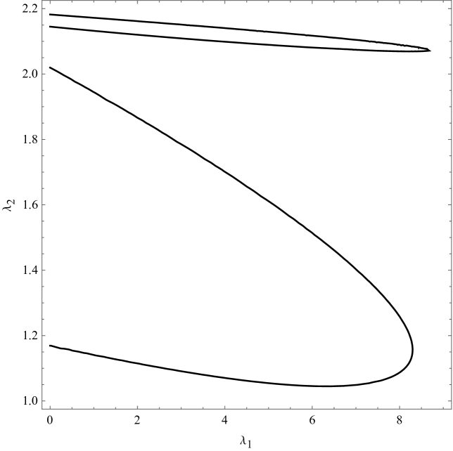
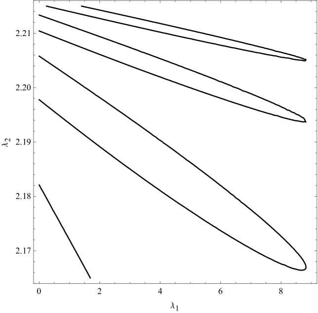
Figure 4: Interaction curves corresponding to different bucking modes for: $\kappa=0.25$ - upper graphs; $\kappa=0.45$ - lower left graphs for lower-order modes; $\kappa=0.45$ - lower right graphs for higher-order modes.

Figure 5 depicts the behavior of (to its maximum value) normalized solution (34) of the linearized problem (28) at the interaction curve branching point $\left(\lambda_{01},\lambda_{02}\right)=\left(8.29796,1.15665\right)$ for $\kappa=0.45,$ see also the lower right graph in Figure 4, as well as for the critical values in its neighborhood on the lower (thick lines) and upper (thin lines) branch. One notices that the shape of linear solution corresponding to the first buckling mode is degenerating into the shape resembling to the second buckling mode as the critical values pass from the lower to the upper branch through the interaction curve branching point, as shown in Figure 5.

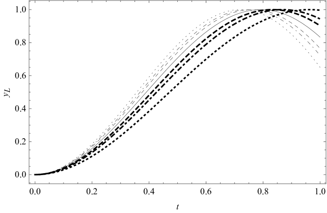
$\!\!\!\!\left(\lambda_{01},\lambda_{02}\right)=$
$(6,1.04544)$ - thick dotted line
$(7.5,1.05978)$ - thick dot-dashed line
$(8,1.08694)$ - thick dashed line
$(8.29796,1.15665)$ - solid line
$(8,1.25843)$ - thin dashed line
$(7.5,1.33932)$ - thin dot-dashed line
$(6,1.51419)$ - thin dotted line

Figure 5: Plots of linear solution $y_{L}$ versus $t$ for non-locality parameter $\kappa=0.45$ for different critical values $(\lambda_{01},\lambda_{02})$.

Post-critical buckling shapes, presented in Figures 6 - 9, are obtained as the numerical solution of system of non-linear equations (5), subject to boundary conditions (6), with $\alpha_{1}=\alpha_{2}=0,\$and either $\lambda_{1}=\lambda_{01}+\Delta\lambda_{1}$ and $\lambda_{2}=\lambda_{02}+\eta^{\prime}\left(\text{$\lambda_{01}$}\right)\Delta\lambda_{1},$ or $\lambda_{1}=\lambda_{01}+\bar{\eta}^{\prime}\left(\text{$\lambda_{02}$}\right)\Delta\lambda_{2}$ and $\lambda_{2}=\lambda_{02}+\Delta\lambda_{2},$ where $\eta^{\prime}$ is given by (32) and $\bar{\eta}^{\prime}$ is obtained analogously to $\eta^{\prime}.$ In the each case of post-buckling modes, the type of bifurcation point is determined according to Theorem 2 by calculating $\varepsilon=\mathrm{sgn\,}c_{3}\;$and $\delta=\mathrm{sgn\,}\left(c_{11}+c_{12}\eta^{\prime}\left(\text{$\lambda_{01}$}\right)\right),$ with $c_{11},$ $c_{12},$ and $c_{3}$ given by (52), (53), and (55). Using Theorem 4, i.e., by calculating the determinant (59), it is also shown that in the each case of post-buckling modes there exists the two-parameter unfolding for the initial displacement, i.e., curvature, assumed as

$$y\left(t\right)=t^{3}-\frac{4}{3}t^{2}+\frac{4}{9}t,\;\;\text{i.e.,}\;\;\frac{1}{\rho_{0}\left(t\right)}=\frac{6t-\frac{8}{3}}{\sqrt{1-\left(3t^{2}-\frac{8}{3}t+\frac{4}{9}\right)^{2}}},$$

regardless of the use of $q_{l}^{\left(2\right)},$ given by (40), or $q_{l}^{\left(4\right)},$ given by (41).

In the case of non-locality parameter $\kappa=0.25<\kappa_{cr},$ the first post-buckling modes, corresponding to the different critical values on the interaction curve from the upper graph in Figure 4, are presented in Figure 6. Their shape strongly resembles to the shape of the first buckling mode of linear solution. Numerical calculation of $\varepsilon=\mathrm{sgn\,}c_{3}$ and $\delta=\mathrm{sgn\,}\left(c_{11}+c_{12}\eta^{\prime}\left(\text{$\lambda_{01}$}\right)\right)$ shows that they are of different sign for both $q_{l}^{\left(2\right)}$ and $q_{l}^{\left(4\right)},$ implying the super-critical bifurcation.

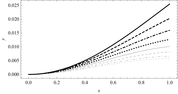
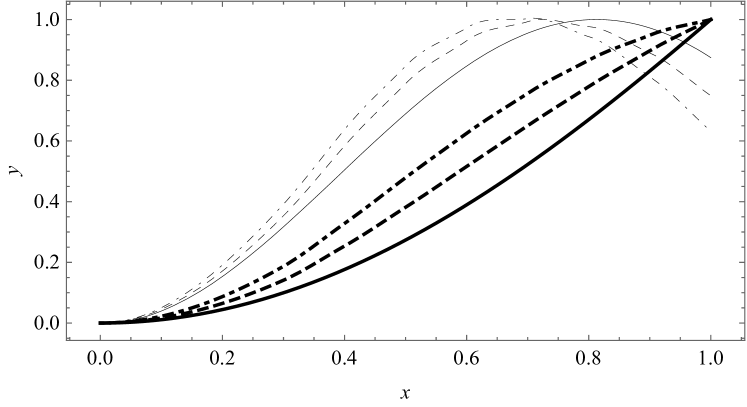
$\!\!\!\!\left(\lambda_{01},\lambda_{02}\right)=$
$(0.05,1.52248)$ - thick solid line
$(2.5,1.33903)$ - thick dashed line
$(5,1.13541)$ - thick dot-dashed line
$(7.5,0.916144)$ - thick dotted line
$(10,0.682732)$ - thin solid line
$(12.5,0.436978)$ - thin dashed line
$(15,0.180736)$ - thin dot-dashed line
$(16.71310,0)$ - thin dotted line

Figure 6: Plots of non-linear solution $y$ versus $x$ for non-locality parameter $\kappa=0.25$ for different critical values $(\lambda_{01},\lambda_{02})$, with $\Delta\lambda_{1}=0.5$.

For the non-locality parameter value of $\kappa=0.45>\kappa_{cr}$ the lower branch of interaction curve from the lower left graph in Figure 4 has a minimum at $\left(\lambda_{01}^{\left(\min\right)},\lambda_{02}^{\left(\min\right)}\right)=\left(6.32271,1.04474\right)$ at which there is a distinct change in the shape of the first post-buckling mode, as noticeable from Figure 7, since for $\lambda_{01}<\lambda_{01}^{\left(\min\right)}$ mode shapes resemble to the shape of the first buckling mode of linear solution (thick lines), while for $\lambda_{01}>\lambda_{01}^{\left(\min\right)}$ mode shapes resemble more to the shape of the second buckling mode of linear solution (thin lines). The post-buckling mode shapes at the minimum and in its neighborhood are shown in Figure 8. Again, the numerical calculation of $\varepsilon$ and $\delta$ shows that they are of different sign for both $q_{l}^{\left(2\right)}$ and $q_{l}^{\left(4\right)},$ implying the super-critical bifurcation.

$\!\!\!\!\left(\lambda_{01},\lambda_{02}\right)=$
$(0.05,1.16776)$ - thick solid line
$(2.5,1.10261)$ - thick dashed line
$(5,1.05447)$ - thick dot-dashed line
$(7,1.04881)$ - thin solid line
$(7.5,1.05978)$ - thin dashed line
$(8.29796,1.15665)$ - thin dot-dashed line

Figure 7: Plots of non-linear solution $y$ versus $x$ for non-locality parameter $\kappa=0.45$ for different critical values $(\lambda_{01},\lambda_{02})$, with $\Delta\lambda_{2}=0.02$.

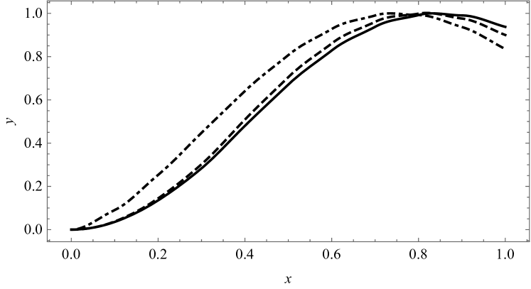
$\!\!\!\!\left(\lambda_{01},\lambda_{02}\right)=$
$(5.75,1.04684)$ - solid line
$(6.32271,1.04474)$ - dashed line
$(6.75,1.04684)$ - dot-dashed line

Figure 8: Plots of non-linear solution $y$ versus $x$ for non-locality parameter $\kappa=0.45$ for different critical values $(\lambda_{01},\lambda_{02})$, with $\Delta\lambda_{1}=0.5$.

The post-buckling mode shapes for the critical values lying on the upper branch of interaction curve from the lower left graph in Figure 4 are presented in Figure 9. Mode shapes corresponding to $\left(\lambda_{01},\lambda_{02}\right)=\left(7.5,1.33932\right)$ and $\left(\lambda_{01},\lambda_{02}\right)=\left(5,1.61161\right)$ resemble to the shape of the first buckling mode of linear solution and $\varepsilon$ and $\delta$ are of different sign implying the super-critical bifurcation, while for $\left(\lambda_{01},\lambda_{02}\right)=\left(2.5,1.82714\right)$ and $\left(\lambda_{01},\lambda_{02}\right)=\left(0.05,2.01637\right)$ $\varepsilon$ and $\delta$ are of the same sign implying the sub-critical bifurcation.

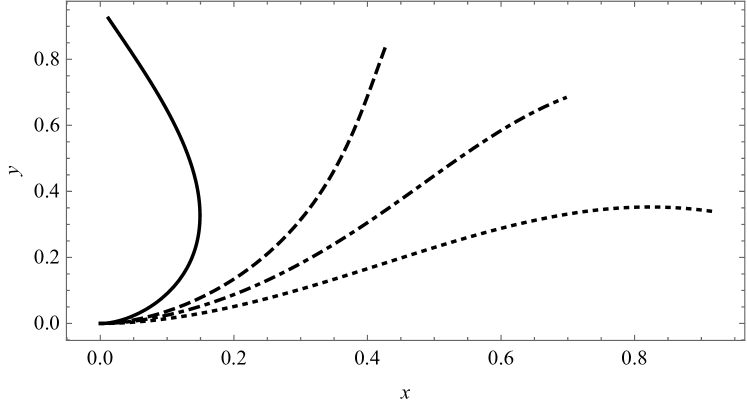
$\!\!\!\!\left(\lambda_{01},\lambda_{02}\right)=$
$(0.05,2.01637)$ - solid line
$(2.5,1.82714)$ - dashed line
$(5,1.61161)$ - dot-dashed line
$(7.5,1.33932)$ - dotted line

Figure 9: Plots of non-linear solution $y$ versus $x$ for non-locality parameter $\kappa=0.45$ for different critical values $(\lambda_{01},\lambda_{02})$, with $\Delta\lambda_{2}=0.02$.

5 Conclusion

Using the bifurcation theory, the static stability problem of cantilevered rotating axially compressed non-local rod is revisited and extended by considering imperfections in shape and loading, represented by the small initial deformation of the rod and vertical force of small intensity acting on rod’s tip. The non-locality effects are included by considering the stress gradient Eringen moment-curvature constitutive relation.

Theorem 1 states that the critical values of angular velocity and intensity of the horizontal axial force acting on rod’s tip, obtained from the implicitly given interaction curve equation (29), represent the bifurcation points for the non-linear equation (13), subject to boundary conditions (18). Theorem 2 uses the Lyapunov-Schmidt reduction method and determines that the problem (10), subject to (12), admits pitchfork bifurcation, while Theorem 4 states that the selected imperfections constitute the two-parameter universal unfolding of the same problem. The obtained results in the case of Bernoulli-Euler moment-curvature constitutive equation reduce to the results obtained in [4].

Numerical treatment of the interaction curve equation (29) shown the interaction curve branching in cases of small value of non-locality parameter for higher modes even if the interaction curve is monotone for the first (or second) mode. The interaction curve branching occurs in cases of large value of non-locality parameter even for the first mode (and higher modes as well). In the case of monotonically decreasing interaction curve, using Theorem 2, it is shown that the pitchfork bifurcation is super-critical, which is also the case on lower branch of interaction curve, while the bifurcation may change to sub-critical on the upper branch. It is also shown, using Theorem 4, that the selected initial deformation and vertical force constitute the two-parameter universal unfolding.

References

[1]
J. Aranda-Ruiz, J. Loya, and J. Fernández-Sáez.
Bending vibrations of rotating nonuniform nanocantilevers using the
Eringen nonlocal elasticity theory.
Composite Structures, 94:2990–3001, 2012.
[2]
B. Arash and Q. Wang.
A review on the application of nonlocal elastic models in modeling of
carbon nanotubes and graphenes.
Computational Materials Science, 51:303–313, 2012.
[3]
T. M. Atanackovic.
Buckling of rotating compressed rods.
Acta Mechanica, 60:49–66, 1986.
[4]
T. M. Atanackovic.
Stability of rotating compressed rod with imperfections.
Mathematical Proceedings of the Cambridge Philosophical
Society, 101:593–607, 1987.
[5]
T. M. Atanackovic.
On the rotating rod with variable cross section.
Archive of Applied Mechanics, 67:447–456, 1997.
[6]
T. M. Atanackovic.
Stability Theory of Elastic Rods.
World Scientific, New Jersay, 1997.
[7]
T. M. Atanackovic and M. Achenbach.
Stability of an extensible rotating rod.
Continuum Mechanics and Thermodynamics, 1:81–95, 1989.
[8]
T. M. Atanackovic, B. N. Novakovic, Z. Vrcelj, and D. Zorica.
Rotating nanorod with clamped ends.
International Journal of Structural Stability and Dynamics,
15:1450050–1–8, 2015.
[9]
T. M. Atanackovic and D. Zorica.
Stability of the rotating compressed nano-rod.
Zeitschrift für angewandte Mathematik und Mechanik,
94:499–504, 2014.
[10]
T. A. Bodnar.
The stability of a compressed rotating rod.
Journal of Applied Mechanics and Technical Physics,
41:745–751, 2000.
[11]
S-N. Chow and J. K. Hale.
Methods of Bifurcation Theory.
Springer-Verlag, Berlin, 1982.
[12]
I. Elishakoff, D. Pentaras, K. Dujat, C. Versaci, G. Muscolino, J. Storch,
S. Bucas, N. Challamel, T. Natsuki, Y. Y. Zhang, C. M. Wang, and
G. Ghyselinck.
Carbon Nanotubes And Nanosensors: Vibrations, Buckling And
Ballistic Impact.
ISTE and John Wiley & Sons, London, New York, 2012.
[13]
M. A. Eltaher, M. E. Khater, and S. A. Emam.
A review on nonlocal elastic models for bending, buckling,
vibrations, and wave propagation of nanoscale beams.
Applied Mathematical Modelling, 40:4109–4128, 2016.
[14]
A. C. Eringen.
Nonlocal Continuum Field Theories.
Springer Verlag, New York, 2002.
[15]
M. Golubitsky and D. Schaeffer.
Singularities and Groups in Bifurcation Theory, volume I.
Springer-Verlag, Berlin, 1985.
[16]
H. Kielhöfer.
Bifurcation Theory. An Introduction with Applications to PDEs.
Springer-Verlag, New York, 2004.
[17]
W. D. Lakin.
On the differential equation of a rapidly rotating slender rod.
Quarterly of Applied Mathematics, 32:11–27, 1974.
[18]
H-T. Thai, T. P. Vo, T-K. Nguyen, and S-E. Kim.
A review of continuum mechanics models for size-dependent analysis of
beams and plates.
Composite Structures, 177:196–219, 2017.
[19]
P. C. Varadi.
Conditions for stability of rotating elastic rods.
Proceedings of the Royal Society A: Mathematical, Physical and
Engineering Sciences, 457:1701–1720, 2001.
[20]
C. Y. Wang.
On the bifurcation solutions of an axially rotating rod.
Quarterly Journal of Mechanics and Applied Mathematics,
35:391–402, 1982.