Problems related to conformal slit-mappings

Abstract.

In this note we discuss some problems related to conformal slit-mappings. On the one hand, classical Loewner theory leads us to questions concerning the embedding of univalent functions into slit-like Loewner chains. On the other hand, a recent result from monotone probability theory motivates the study of univalent functions from a probabilistic perspective.

1. Introduction

Let $\mathbb{D}=\{z\in\mathbb{C}\,|\,|z|<1\}$ be the unit disc in the complex plane. The class $S$ is defined as the set of all univalent (=holomorphic and injective) $f:\mathbb{D}\to\mathbb{C}$ with $f(0)=0$ and $f^{\prime}(0)=1.$
The famous Bieberbach conjecture states that if $f(z)=z+\sum_{n\geq 2}a_{n}z^{n}$ belongs to $S$, then $|a_{n}|\leq n$ for all $n\geq 2.$ Bieberbach himself proved the case $n=2$. Later on, Loewner introduced a new method to handle the case $n=3$ ([Löw23]). His approach has been extended and generalized to what is now called Loewner theory, and it was also used in the final proof of the conjecture by de Branges.

Definition 1.1.

A (normalized radial) Loewner chain is a family $(f_{t})_{t\geq 0}$ of univalent functions $f_{t}:\mathbb{D}\to\mathbb{C}$ with $f_{t}(0)=0$, $f_{t}^{\prime}(0)=e^{t}$, and $f_{s}(\mathbb{D})\subseteq f_{t}(\mathbb{D})$ whenever $s\leq t.$ We say that a function $f\in S$ can be embedded into a Loewner chain if there exists a Loewner chain $(f_{t})$ with $f_{0}=f$.

A Loewner chain is differentiable almost everywhere and satisfies Loewner’s partial differential equation:

(1.1) $$\frac{\partial f_{t}}{\partial t}(z)=zf^{\prime}_{t}(z)p(t,z)\quad\text{ for a.e. $t\geq 0$ and all $z\in\mathbb{D}$}.$$

The function $p:[0,\infty)\times\mathbb{D}\to\mathbb{C}$ is a so called Herglotz vector field, i.e., for almost every $t\geq 0$, $p(t,\cdot)$ maps $\mathbb{D}$ holomorphically into the right half-plane and $0$ onto $1$, and for every $z\in\mathbb{D}$, $t\mapsto p(t,z)$ is measurable. Conversely, every Herglotz vector field uniquely defines a Loewner chain. We refer to [Pom75, Chapter 6] for these statements. Pommerenke proved the following nice result.

Theorem 1.2 (Theorem 6.1 in [Pom75]).

Every $f\in S$ can be embedded into a Loewner chain.

Remark 1.3.

Loewner chains can also be regarded in $\mathbb{C}^{n}$ or on complex manifolds. We refer to [Fia17] for embedding problems of biholomorphic mappings on the Euclidean unit ball in $\mathbb{C}^{n}$ and to the recent result from [FW18], which shows that the analogue of Pommerenke’s theorem fails in higher dimensions.

A slit in $\mathbb{C}$ is a Jordan curve $\Gamma$ connecting some $z_{0}\in\mathbb{C}$ to $\infty.$ We call $f\in S$ a slit mapping if $f(\mathbb{D})$ is the complement of a slit. Loewner’s original result focuses on slit mappings.

Theorem 1.4 ([Löw23]).

Let $f\in S$ be a slit mapping. Then $f$ can be embedded into exactly one Loewner chain $\{f_{t}\}_{t\geq 0}$. There exists a continuous $\kappa:[0,\infty)\to\partial\mathbb{D}$ such that

(1.2) $$\frac{\partial f_{t}}{\partial t}(z)=zf^{\prime}_{t}(z)\frac{\kappa(t)-z}{\kappa(t)+z}\quad\text{ for every $t\geq 0.$}$$

Remark 1.5.

Each $f_{t}$ maps $\mathbb{D}$ onto the complement of a subslit. Denote by $\gamma(t)$ the tip of this slit. Then, for each $t\geq 0$, $f_{t}^{-1}$ can be extended continuously to $\gamma(t)$ and the driving function $\kappa$ can be written as

(1.3) $$\kappa(t)=f_{t}^{-1}(\gamma(t)).$$

In this paper, we address some embedding problems in Section 2, which are all motivated by Theorem 1.4. In Section 3, we look at slit mappings from a probabilistic point of view.

2. Embedding problems

Note that in Theorem 1.4, the Loewner chain $(f_{t})$ is uniquely determined and differentiable everywhere (right-differentiable at $t=0$). This leads us to a couple of subclasses of $S$ related to embedding problems. Before defining these classes, we point out how to recover the first element of a Loewner chain from the Loewner equation.

Loewner’s ordinary differential equation is the following analogue to (1.1):

(2.1) $$\frac{\partial\varphi_{s,t}}{\partial t}(z)=-\varphi_{s,t}(z)\cdot p(t,\varphi_{s,t}(z))\quad\text{ for a.e. $t\geq s$ with $\varphi_{s,s}(z)=z$ }$$

for all $z\in\mathbb{D}$. The solution $(\varphi_{s,t})_{0\leq s\leq t}$ is a family of univalent functions $\varphi_{s,t}:\mathbb{D}\to\mathbb{D}$.

If $(f_{t})$ satisfies (1.1), then $\varphi_{s,t}$ is given by $\varphi_{s,t}=f_{t}^{-1}\circ f_{s}$ and the functions $(\varphi_{s,t})_{0\leq s\leq t}$ are thus called the transition mappings of the Loewner chain.
Conversely, if $\varphi_{s,t}$ is the solution to (2.1), then, for every $s\geq 0$,

(2.2) $$f_{s}=\lim_{t\to\infty}e^{t}\varphi_{s,t}$$

locally uniformly on $\mathbb{D}$; see [Pom75, Theorem 6.3]. Thus, the first element of a Loewner chain can also be regarded as the infinite time limit of the solution of (2.1) for $s=0$.

Remark 2.1.

If $D\subset\mathbb{D}$ is a simply connected domain with $0\in D$, then there exists $T>0$ and a Herglotz vector field $p(t,z)$ such that the solution $\varphi_{0,t}$ of (2.1) satisfies $\varphi_{0,T}(\mathbb{D})=D$. This follows basically from Theorem 1.2 and is mentioned as an exercise in [Pom75, Section 6.1, Problem 3].
The above statement is equivalent to the following: Let $f\in S$ such that $f(\mathbb{D})$ is bounded. Then there exists $T>0$ and a Loewner chain $(f_{t})$ such that $f_{0}=f$ and $f_{T}(\mathbb{D})=e^{T}\mathbb{D}$.

2.1. Differentiability

Let us call a Loewner chain $(f_{t})$ differentiable if $t\mapsto f_{t}(z)$ is differentiable at every $t\geq 0$ for every $z\in\mathbb{D}$. We define the class

$$S_{d}:=\{f\in S\,|\,\text{$f$ can be embedded into a differentiable Loewner chain}\}.$$

Every slit mapping belongs to $S_{d}$ due to Theorem 1.4. Another simple example can be obtained as follows. Assume that $f(\mathbb{D})$ is bounded by a closed Jordan curve. Then we can first connect this curve to $\infty$ by a Jordan arc, and now erase the two curves to obtain a Loewner chain satisfying (1.2).

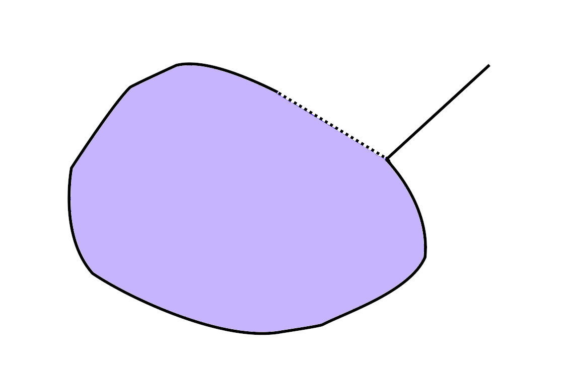
Figure 1. A Jordan domain (blue) connected to $\infty$ by a Jordan arc.

Suppose that $f\in S$ maps $\mathbb{D}$ onto the complement of two disjoint slits. Then we can embed $f$ into a Loewner chain by erasing a piece of the first slit in some time interval $[0,T_{1}]$, then a piece of the second slit in an interval $[T_{1},T_{2}]$, etc. In this case, $(f_{t})$ is not differentiable at $t=T_{1}$. However, one can also erase the slits simultaneously and then the corresponding Loewner chain is differentiable everywhere. This is true for any $f$ mapping $\mathbb{D}$ onto the complement of finitely many slits. These statements follow from [Böh16, Theorem 2.31].

However, not every $f\in S$ belongs to $S_{d}$.

Theorem 2.2.

There exists $f\in S\setminus S_{d}$.

Proof.

Let $D\subsetneq\mathbb{C}$ be a simply connected domain with $0\in D$ and let $f:\mathbb{D}\to D$ be the conformal mapping with $f(0)=0$ and $f^{\prime}(0)>0$. In what follows, the number $c=f^{\prime}(0)$ will be called the capacity of $D$ and $f$ its normalized conformal mapping.
Koebe’s one-quarter theorem implies that $D$ contains a disc centered at $0$ with radius $c/4$, see [Dur83, Theorem 2.3].

Consider the topological sine $J=\{x+i\sin(1/x)\,|\,x>0\}\cup\{ix\,|\,x\in[-1,1]\}.$ We connect $J$ by a Jordan curve $\beta_{1}$ starting at $i$ and staying in $\mathbb{C}\setminus J$ otherwise. We do the same for a second curve $\beta_{2}$ starting at $-i;$ see the figure below.

Figure 2. The sets $J,\beta_{1},\beta_{2}$.

Now we translate the set $J\cup\beta_{1}\cup\beta_{2}$ such that $0$ belongs to the complement, and then scale it (we keep the notation for these new sets) such that $\mathbb{C}\setminus(J\cup\beta_{1})$ has capacity $1$. Denote by $h_{1}$ the normalized conformal mapping of $\mathbb{C}\setminus(J\cup\beta_{1})$.

Next we look at the domain $\mathbb{C}\setminus(J\cup\beta_{2})$. If we change it by extending or shortening the curve $\beta_{2}$, then the capacity changes continuously due to Carathéodory’s kernel theorem. We can extend $\beta_{2}$ to a neighbourhood of $0$ to make the capacity as small as we like, due to Koebe’s one-quarter theorem. Furthermore, the domain $\mathbb{C}\setminus J$ has a capacity larger than $1$.
Hence, the intermediate value theorem implies that we can extend or shorten $\beta_{2}$ (we keep the same notation) such that $\mathbb{C}\setminus(J\cup\beta_{2})$ has capacity $1$. Let $h_{2}$ be the normalized conformal mapping of $\mathbb{C}\setminus(J\cup\beta_{2})$.

Then $h_{1},h_{2}\in S$ and we can use Theorem 1.2 to obtain a Loewner chain $\{f_{1,t}\}_{t\geq 0}$ with $f_{1,0}=h_{1}$ and a Loewner chain $\{f_{2,t}\}_{t\geq 0}$ with $f_{2,0}=h_{2}.$ It is easy to see that $f_{1,t}$ is unique, as $f_{1,t}$ must erase the curve $\beta_{1}$ for $t\in[0,T]$ for some $T>0.$ The function $f_{1,T}$ maps $\mathbb{D}$ onto $\mathbb{C}\setminus J.$ For $t>T,$ the Loewner chain erases the topological sine. Similarly, $f_{2,t}$ is unique and $f_{1,t}=f_{2,t}$ for all $t\geq T.$

We show that there exist continuous $\kappa_{j}:[0,T)\cup(T,\infty)\to\partial\mathbb{D}$ such that $f_{j,t}$ satisfies (1.2) for every $t\in[0,T)\cup(T,\infty).$ This is clear for $t>T$, as $f_{j,t}$ is simply a slit mapping then and we can apply Theorem 1.4.
Next it follows from [Pom92, Proposition 2.14] that $f_{1,T}^{-1}(\beta_{j})=f_{2,T}^{-1}(\beta_{j})$ is a curve in $\mathbb{D}$ with one endpoint $K_{j}$ in $\partial\mathbb{D}$. Moreover, [Pom92, Proposition 2.14] also states that $K_{1}\not=K_{2}$.
Now we conclude that there exist continuous $\kappa_{j}:[0,T]\to\partial\mathbb{D}$ such that $f_{j,t}$ satisfies (1.2) on $[0,T]$ (with a left-derivative for $t=T$). Furthermore, $\kappa_{j}(T)=K_{j}$. This follows readily from the proof of Loewner’s theorem. Alternatively, we can regard the family $(f_{j,T}^{-1}\circ f_{j,T-t})_{t\in[0,T]}$. It describes the growth of the slit $f_{1,T}^{-1}(\beta_{j})$ and satisfies the time-reversed version of Loewner’s differential equation with the Herglotz vector field as in (1.2) with continuous driving function, see [Böh16, Theorem 2.22]. It follows that $f_{j,t}$ satisfies (1.2) with continuous $\kappa_{j}:[0,T]\to\partial\mathbb{D}$ on $[0,T]$.

Now we show that either $f_{1,t}$ or $f_{2,t}$ is not differentiable at $t=T$. Assume the opposite and fix some $z\in\mathbb{D}\setminus\{0\}$. Then $t\mapsto h_{t}(z):=f_{1,t}(z)-f_{2,t}(z)$ is differentiable for all $t>0.$ We have $\frac{d}{dt}h_{t}(z)=0$ for all $t>T.$
Furthermore, we see that the limit

$$\lim_{t\uparrow T}\frac{d}{dt}h_{t}(z)=2z^{2}f_{T}^{\prime}(z)\frac{K_{1}-K_{2}}{(K_{1}+z)(K_{2}+z)}$$

exists and is different from $0.$ Hence, $\frac{d}{dt}h_{t}(z)$ has a first kind discontinuity at $t=T.$ This is a contradiction to Darboux’s theorem (applied to the real or imaginary part of $\frac{d}{dt}h_{t}(z)$). ∎

We remark that there is a wide range of examples of $f\in S_{d}$ whose boundary $\partial f(\mathbb{D})$ is not locally connected, i.e., $f$ does not have a continuous extension to $\overline{\mathbb{D}}$. In fact, typical known subclasses of $S$ in the theory of univalent functions (e.g. close-to-convex functions) are contained in $S_{d}$ (see e.g. Section 3.4 in [Hot]).

2.2. Unique embeddings

Next we define

$$S_{u}:=\{f\in S\,|\,\text{$f$ can be embedded into exactly one Loewner chain}\}.$$

Note that all slit mappings belong to $S_{u}$. Clearly, there is only one way how to remove a slit by a Loewner chain. The proof of Theorem 2.2 implies that there exists $f\in S_{u}$ which is not a slit mapping. Roughly speaking, the complement $\mathbb{C}\setminus f(\mathbb{D})$ must be “thin” for $f\in S_{u}$. One might think that $\mathbb{C}\setminus f(\mathbb{D})=\partial f(\mathbb{D})$ for such mappings. However, this is not true due to the next example.

Example 2.3.

Let $f\in S$ such that $\partial f(\mathbb{D})$ is an infinite spiral $\gamma:(0,1)\to\mathbb{C}$ surrounding a disc $D$, i.e. $\gamma(t)\to\infty$ as $t\downarrow 0$ and the set of all accumulation points $\lim_{n\to\infty}\gamma(t_{n})$ with $t_{n}\uparrow 1$ is equal to the circle $\partial D$. Then $f\in S_{u}$ and $\partial f(\mathbb{D})\subsetneq\mathbb{C}\setminus f(\mathbb{D})$, as the interior of $D$ does not belong to $\partial f(\mathbb{D})$.

Figure 3. Infinite spiral enclosing a disc.

The following lemma is quite useful for constructing Loewner chains.

Lemma 2.4.

Let $f\in S$ and $D=f(\mathbb{D})$. Assume that $E\subsetneq\mathbb{C}$ is a simply connected domain with $D\subsetneq E$. Then there exists a Loewner chain $(f_{t})$ and $T>0$ such that $f_{0}=D$ and $f_{T}=E$.

Proof.

Let $g:\mathbb{D}\to E$ be a conformal mapping with $g(0)=0$ and $g^{\prime}(0)=e^{T}$ for some $T>0$. There exists a Loewner chain $(h_{t})_{t}$ such that $h_{0}=e^{-T}g$ due to Theorem 1.2. Let $p_{1}(t,z)$ be the corresponding Herglotz vector field.
Write $f=g\circ\varphi$. By Remark 2.1, there exists a Herglotz vector field $p_{2}(t,z)$ such that the solution $\varphi_{0,t}$ of (2.1) satisfies $\varphi_{0,T}=\varphi$. Now consider the Herglotz vector field $p(t,z)$ defined by

$$p(t,z)=p_{2}(t,z)\quad\text{for $t\leq T$ \quad and}\quad p(t,z)=p_{1}(t-T,z)\quad\text{for $t>T$ and all $z\in\mathbb{D}$}.$$

Let $(f_{t})$ be the corresponding Loewner chain with transition mappings $(\psi_{s,t})$. Then $\psi_{0,t}=\varphi_{0,t}$ for all $t\in[0,T]$. We have $f_{0}=f_{T}\circ\varphi_{0,T}=f_{T}\circ\varphi$ and $f_{T}=\lim_{t\to\infty}e^{t}\psi_{T,t}=e^{T}h_{0}=g$. Hence, $f_{T}(\mathbb{D})=E$ and $f_{0}(\mathbb{D})=(f_{T}\circ\varphi)(\mathbb{D})=f(\mathbb{D})=D$. ∎

Theorem 2.5.

Let $f\in S_{u}$ and let $D=f(\mathbb{D})$. Then $D$ has the following properties:

• $D$ is unbounded.

• $\partial D$ is connected.

• Let

  $$\mathcal{C}(D)=\{C\subset\partial D\,|\,\text{$C$ is connected, unbounded, and closed}\}.$$

  If $C_{1},C_{2}\in\mathcal{C}(D)$, then $C_{1}\subseteq C_{2}$ or $C_{2}\subseteq C_{1}$.

Proof.

• Assume that $D$ is bounded. Then we can embed $f$ into a Loewner chain $(f_{t})$ such that $f_{T}(\mathbb{D})=e^{T}\mathbb{D}$ for some $T>0$, see Remark 2.1. As $\mathbb{D}$ can be embedded into many Loewner chains, we conclude $f\not\in S_{u}$, a contradiction.

• Due to (a), the set $\mathcal{C}(D)$ is non-empty. Let $C_{1},C_{2}\in\mathcal{C}(D)$. Let $(f_{t})$ be the unique Loewner chain with $f_{0}=f$ and let $D_{t}=f_{t}(\mathbb{D})$.
  Let $E_{1}$ and $E_{2}$ be the connected component of $\mathbb{C}\setminus C_{1}$ and $\mathbb{C}\setminus C_{2}$ respectively containing $D$.
  Then $E_{1}$ and $E_{2}$ are simply connected domains and due to Lemma 2.4, there exist $T_{1},T_{2}$ such that $E_{1}=D_{T_{1}}$, $E_{2}=D_{T_{2}}$. This implies $E_{1}\subseteq E_{2}$ or $E_{2}\subseteq E_{1}$, say we have $E_{1}\subseteq E_{2}$. We need to show that $C_{2}\subseteq C_{1}$. Assume that this is not true. Then there exists a point $p\in C_{2}$ and $p\not\in C_{1}$.
  Now note that $\partial D\setminus C_{1}\subseteq E_{1}$. Hence $p\in E_{1}$ and thus $p\in E_{2}$. But $p$ also belongs to $C_{2}$ and thus to the complement of $E_{2}$, a contradiction.

• Assume that $\partial D$ has at least two connected components $C_{1},C_{2}$. Then both components are unbounded, otherwise $D$ would not be simply connected. Hence, $C_{1},C_{2}\in\mathcal{C}(D)$ with $C_{1}\cap C_{2}=\emptyset$, a contradiction to (c).

∎

In case $f\in S_{u}$ maps $\mathbb{D}$ onto the complement of a slit $\gamma$, the elements of $\mathcal{C(D)}$ are simply subslits of $\gamma$. We see that in the general case, each $p\in\partial D$ is connected to $\infty$ within $\partial D\cup\{\infty\}$ in a unique way, i.e. there is a smallest connected closed subset of $\partial D\cup\{\infty\}$ containing $p$ and $\infty$.

2.3. Slit equation

Finally, we can look at the special form of Loewner’s differential equation appearing in Theorem 1.4.

$$S^{1}_{s}:=\{f\in S\,|\,\text{$f$ can be embedded into \eqref{slit_LE} for continuous $\kappa$}\}\subsetneq S_{d}.$$

If $f\in S$ is a two-slit mapping, then $f\in S_{d}$ but $f\not\in S^{1}_{s}$, which shows that $S^{1}_{s}$ is a proper subset of $S_{d}$.

The class $S^{1}_{s}$ (and its variations) has been studied intensively in the literature.

• Pommerenke characterizes Loewner chains corresponding to $S^{1}_{s}$ via the “local growth property”, see [Pom66, Theorem 1].

• Every slit mapping belongs to $S^{1}_{s}$. However, continuous driving functions can also create non-slit mappings. For example, every $f\in S$ such that $f(\mathbb{D})$ is a Jordan domain belongs to $S^{1}_{s}$ due to the Loewner chain depicted in Figure 1. One can even generate spacefilling curves by continuous $\kappa$, see [LR12].
  The set of all continuous driving functions that correspond to slits in this way is not known explicitly. However, there are several partial results into that direction. Roughly speaking, if $\kappa$ is smooth enough, e.g. continuously differentiable, then $f$ is a slit mapping. We refer to the recent work [ZZ18] and the references therein for such results.

• Loewner’s slit equation can be seen as a machinery transferring a simple curve $\Gamma$ into a continuous function $\kappa:[0,\infty)\to\partial\mathbb{D}$. This process

  $$\Gamma\longrightarrow\kappa$$

  encodes “difficult” two-dimensional objects into one-dimensional ones. It seems that this relationship is both rather mysterious and (therefore) quite powerful. In case of the celebrated Schramm-Loewner evolution, certain planar random curves, whose distributions are not easy to understand, are simply transferred into $\kappa(t)=e^{i\sqrt{\kappa}B_{t}}$, where $\kappa\geq 0$ is a parameter and $B_{t}$ is a standard Brownian motion. For an introduction to SLE, we refer to [Law05].

We obtain a second class by requiring that (1.2) should hold only almost everywhere.

$$S^{2}_{s}:=\{f\in S\,|\,\text{$f$ can be embedded into \eqref{slit_LE} for measurable $\kappa$}\}.$$

Recall that a domain $D\subset\mathbb{C}$ is simply connected if and only if $\hat{\mathbb{C}}\setminus D$ is connected. If, in addition, $\hat{\mathbb{C}}\setminus D$ is pathwise connected, then one can erase slits in the complement of $D$. Pommerenke constructed a Loewner chain in this way to obtain the following result.

Theorem 2.6 (Theorem 2 in [Pom66]).

Let $f\in S$ such that $\hat{\mathbb{C}}\setminus f(\mathbb{D})$ is pathwise connected. Then $f\in S^{2}_{s}$.

2.4. Problems

Thinking of the idea of the proof of Theorem 2.6, we are led to the following question.

Problem 2.7.

Let $f\in S$ such that $\hat{\mathbb{C}}\setminus f(\mathbb{D})$ is pathwise connected. Is it possible to embed $f$ into a differentiable Loewner chain by simultaneously erasing slits in the complement?

Problem 2.8.

Pommerenke asks in [Pom66]: Is $S=S^{2}_{s}$?

This question is interesting from a control theoretic point of view.

Denote by $\mathcal{P}$ the Carathéodory class of all holomorphic functions $p:\mathbb{D}\to\mathbb{C}$ with $\text{Re}(p(z))>0$ for all $z\in\mathbb{D}$ and $p(0)=1$. The class $\mathcal{P}$ can be characterized by the Riesz-Herglotz representation formula:

$$\mathcal{P}=\left\{\int_{\partial\mathbb{D}}\frac{u+z}{u-z}\,\mu(du)\,|\,\mu\;\text{is a probability measure on $\partial\mathbb{D}$}\right\}.$$

The extreme points of the class $\mathcal{P}$ are thus given by all functions of the form $\frac{u+z}{u-z}$ for some $u\in\partial\mathbb{D}$. Hence, in view of (2.2), a result like $S=S^{2}_{s}$ could be interpreted as a “bang-bang principle” for the Loewner equation.

Problem 2.9.

Let $f\in S_{u}$ be embedded into its unique Loewner chain $(f_{t})$. How does the Loewner equation for $(f_{t})$ look like?

Note that an example of $f\in S_{u}$ whose Loewner equation does not have the form (1.2) for measurable $\kappa$ would prove $S\not=S^{2}_{s}$.

Problem 2.10.

Let $f\in S$ such that $D=f(\mathbb{D})$ satisfies $(a)$-$(c)$ from Theorem 2.5. Is it true that $f\in S_{u}$?

Problem 2.11.

Is it true that the set $S_{u}\cap S_{d}$ contains only slit-mappings?

Problem 2.12.

Let $f\in S$ but $f\not\in S_{u}$. Is it true that $f$ can be embedded into infinitely (uncountably) many Loewner chains?

3. Measures related to univalent slit mappings

Holomorphic functions $f:\mathbb{D}\to\mathbb{C}$ also arise in probability theory. Such mappings encode probability measures $\mu$ on the unit circle $\partial\mathbb{D}$ or on $\mathbb{R}$. The univalence of such functions has a certain meaning in non-commutative probability theory, which will be explained in Section 3.2.

This correspondence motivates two questions:
How can the property that $f(\mathbb{D})$ has the form $\mathbb{D}\setminus\gamma$, where $\gamma$ is a simple curve, be translated into properties of the measure $\mu$?
How are the questions from Section 2 translated if we pass from non-commutative to classical probability theory?

Instead of the unit disc and the normalization $f(0)=0$, we prefer to use the upper half-plane $\mathbb{H}=\{z\in\mathbb{C}\,|\,\text{Im}(z)>0\}$ and a normalization at the boundary point $\infty$. Then the probability measures will be supported on $\partial\mathbb{H}=\mathbb{R}$.

We give a partial answer to the first question in Section 3.1. In Section 3.2 we address the second question and explain the deeper connection of univalent mappings to non-commutative probability theory.

3.1. Univalent Cauchy transforms

Let $\gamma:[0,1]\to\overline{\mathbb{H}}$ be a simple curve with $\gamma(0)\in\mathbb{R}$ and $\gamma(0,1]\subset\mathbb{H}$. Then there exists a unique conformal mapping $f:\mathbb{H}\to\mathbb{H}\setminus\gamma(0,1]$ having the hydrodynamic normalization

$$f(z)=z-\frac{c}{z}+\mathcal{O}(|z|^{-2})$$

for some $c>0$ as $z\to\infty$. The value $c$ is also called the half-plane capacity of the slit.

The Cauchy transform (or Stieltjes transform) of a probability measure $\mu$ on $\mathbb{R}$ is given by

$$G_{\mu}(z)=\int_{\mathbb{R}}\frac{1}{z-t}\,\mu(dt),\qquad z\in\mathbb{C}\setminus\mathbb{R}.$$

We define the $F$–transform of $\mu$ simply as $F_{\mu}:\mathbb{H}\to\mathbb{H},F_{\mu}(z):=1/G_{\mu}(z)$. $F$-transforms can be characterized in the following way.

Theorem 3.1 (Proposition 2.1 and 2.2 in [Maa92]).

Let $F\colon\mathbb{H}\to\overline{\mathbb{H}}$ be holomorphic. Then the followings are equivalent.

• There exists a probability measure $\mu$ on $\mathbb{R}$ such that $F=F_{\mu}$.

• $\lim_{y\to\infty}\frac{F(iy)}{iy}=1$.

• $F$ has the Pick-Nevanlinna representation

  $$F(z)=z+b+\int_{\mathbb{R}}\frac{1+tz}{t-z}\rho({\rm d}t),$$

  where $b\in\mathbb{R}$ and $\rho$ is a finite, non-negative Borel measure on $\mathbb{R}$.

We conclude that every univalent slit mapping $f:\mathbb{H}\to\mathbb{H}\setminus\gamma(0,1]$ with hydrodynamic normalization is the $F$-transform of a probability measure $\mu$, i.e. $f=F_{\mu}$. We are thus led to the problem of characterizing those $\mu$ whose $F$-transforms are univalent slit mappings.

Consider again an arbitrary probability measure $\mu$ on $\mathbb{R}$. Due to Fatou’s theorem, the following radial limits exist almost everywhere on $\mathbb{R}$:

$$\hat{\mathcal{H}}_{\mu}(x):=\lim_{\varepsilon\downarrow 0}\hat{\mathcal{H}}_{\varepsilon,\mu}(x),\quad\hat{\mathcal{H}}_{\varepsilon,\mu}(x):=\frac{1}{\pi}\text{Re}\;G_{\mu}(x+i\varepsilon).$$

The Hilbert transform of $\mu$ is defined by

$$\mathcal{H}_{\mu}(x):=\lim_{\varepsilon\downarrow 0}\mathcal{H}_{\varepsilon,\mu}(x),\quad\mathcal{H}_{\varepsilon,\mu}(x):=\frac{1}{\pi}\int_{|x-t|>\varepsilon}\frac{1}{x-t}\,\mu(dt).$$

$\mathcal{H}_{\mu}$ is also defined for almost every $x\in\mathbb{R}$. The Sokhotski-Plemelj formula implies that $\mathcal{H}_{\mu}(x)$ and $\hat{\mathcal{H}}_{\mu}(x)$ coincide. As this equality is usually stated to hold almost everywhere on $\mathbb{R}$ (see [Sch12, Theorem F.3] or [CMR06, Sections 2.5, 3.8]), we include the short proof of the pointwise equality needed in our situation.

Lemma 3.2.

Let $\mu$ be an absolutely continuous probability measure with compact support and continuous density $f(x)dx$. Let $x\in\mathbb{R}$. Then $\mathcal{H}_{\mu}(x)$ exists if and only if $\hat{\mathcal{H}}_{\mu}(x)$ exists.
If these limits exist, then $\mathcal{H}_{\mu}(x)=\hat{\mathcal{H}}_{\mu}(x)$.

Proof.

First, we consider the relevant integrals and change $t$ to $t=x+\varepsilon u$, which gives

$$\int_{\mathbb{R}}\frac{1}{x-t+i\varepsilon}f(t)\,dt-\int_{|x-t|>\varepsilon}\frac{1}{x-t}f(t)\,dt$$

$$= \int_{\mathbb{R}}\frac{f(x+\varepsilon u)\varepsilon du}{-\varepsilon u+i\varepsilon}-\int_{|\varepsilon u|>\varepsilon}\frac{f(x+\varepsilon u)\varepsilon du}{-\varepsilon u}=\int_{\mathbb{R}}\left(\frac{1}{i-u}+\chi_{|u|>1}\frac{1}{u}\right)\,f(x+\varepsilon u)du.$$

Denote the function in parentheses by $g(u)$. For $|u|\leq 1$, we have $|g(u)|=\frac{1}{|i-u|}\leq 1$, and if $|u|>1$, then $|g(u)|=\frac{1}{|i-u||u|}\leq\frac{1}{|u|^{2}}.$ So $g$ is integrable and a direct calculation yields $\int_{\mathbb{R}}g(u)du=-i\pi$. Let $[a,b]$ be a compact interval containing the support of $\mu$. Then $|f(x+\varepsilon u)-f(x)|$ is uniformly bounded by $2\max_{t\in[a,b]}|f(t)|$ and the dominated convergence theorem implies that

$$\int_{\mathbb{R}}(f(x+\varepsilon u)-f(x))g(u)\,du\to 0$$

as $\varepsilon\to 0$. Hence, $\text{Re}\int_{\mathbb{R}}f(x+\varepsilon u)g(u)\,du\to 0$ as $\varepsilon\to 0$. So, $\lim_{\varepsilon\downarrow 0}\hat{\mathcal{H}}_{\varepsilon,\mu}(x)$ exists if and only if $\lim_{\varepsilon\downarrow 0}\mathcal{H}_{\varepsilon,\mu}(x)$ exists, and if these limits exist, then they coincide. ∎

We first look at the case where the slit does not start at $0$.

Theorem 3.3.

Let $\mu$ be a probability measure on $\mathbb{R}$ such that $F_{\mu}$ is univalent.
Then $F_{\mu}$ maps $\mathbb{H}$ conformally onto $\mathbb{H}\setminus\gamma$, where $\gamma$ is a slit starting at $C\in\mathbb{R}\setminus\{0\}$, if and only if the following conditions are satisfied:

• $\operatorname{supp}\mu=\{x_{0}\}\cup[a,b]$, where $\mu$ has a continuous density $d(x)$ on the compact interval $[a,b]$ and an atom at some $x_{0}\in\mathbb{R}\setminus[a,b].$ Furthermore, $d(a)=d(b)=0$ and $d(x)>0$ in $(a,b)$.

• $\mathcal{H}_{\mu}$ is defined and continuous on $\mathbb{R}\setminus\{x_{0}\}$ with $\mathcal{H}_{\mu}(a)=\mathcal{H}_{\mu}(b)=\frac{1}{\pi C}$.

• There exists a decreasing homeomorphism $h:[a,b]\to[a,b]$ with

  $$d(h(x))=d(x)\qquad\text{and}\qquad\mathcal{H}_{\mu}(h(x))=\mathcal{H}_{\mu}(x)$$

  for all $x\in[a,b]$.

Proof.

“$\Longrightarrow$”:
As the domain $\mathbb{H}\setminus\gamma$ has a locally connected boundary, the mapping $F_{\mu}$ can be extended continuously to $\overline{\mathbb{H}};$ see [Pom92, Theorem 2.1].
There exists an interval $[a,b]$ such that $F_{\mu}([a,b])=\gamma$ and there is a unique $u\in(a,b)$ such that $F_{\mu}(u)$ is the tip of the slit. All points $[a,u]$ correspond to the left side, all points $[u,b]$ to the right side of $\gamma.$ (This orientation follows from the behaviour of $F_{\mu}(x)$ as $x\to\pm\infty.$) Hence, there exists a unique homeomorphism $h:[a,b]\to[a,b]$ with $h(u)=u,$ $h[a,u]=[u,b]$ such that $F_{\mu}(h(x))=F_{\mu}(x)$ for all $x\in[a,b].$
Furthermore, $F_{\mu}$ has exactly one zero $x_{0}\in\mathbb{R}\setminus[a,b]$ on $\mathbb{R}$, as the slit does not start at $0$. As $C=F_{\mu}(a)=F_{\mu}(b)$, we have $x_{0}<a$ if and only if $C>0$.

It follows from the Stieltjes-Perron inversion formula, see [Sch12, Theorems F.2, F.6], that $\operatorname{supp}\mu=\{x_{0}\}\cup[a,b]$ and that $\mu$ is absolutely continuous on $[a,b]$ and its density $d(x)$ satisfies

$$d(x)=\lim_{\varepsilon\to 0}-\frac{1}{\pi}\text{Im}(1/F_{\mu}(x+i\varepsilon))=-\frac{1}{\pi}\text{Im}(1/F_{\mu}(x)).$$

Hence, $d(h(x))=d(x)$ for all $x\in[a,b]$, $d(x)>0$ on $(a,b)$, and $d(a)=d(b)=0$.
Let $\lambda=\mu(\{x_{0}\})$. Then we have

$$\frac{1}{\pi}\text{Re}\left(1/F_{\mu}(x)\right)=\hat{\mathcal{H}}_{\mu}(x)=\hat{\mathcal{H}}_{d}(x)+\frac{\lambda}{\pi(x-x_{0})}=\mathcal{H}_{d}(x)+\frac{\lambda}{\pi(x-x_{0})}=\mathcal{H}_{\mu}(x)$$

for every $x\in\mathbb{R}\setminus\{x_{0}\}$ due to Lemma 3.2. Here, $\mathcal{H}_{d}$ and $\hat{\mathcal{H}}_{d}$ are defined by replacing $\mu(dt)$ by $d(t)dt$ in the integration, and formally, we apply Lemma 3.2 to the probability measure defined by the density $d(t)/(1-\lambda)$.
Thus $\mathcal{H}_{\mu}(x)$ is continuous on $\mathbb{R}\setminus\{x_{0}\}$, $\mathcal{H}_{\mu}(a)=\mathcal{H}_{\mu}(b)=\frac{1}{\pi C}$, and $\mathcal{H}_{\mu}(h(x))=\mathcal{H}_{\mu}(x)$ on $[a,b]$.

“$\Longleftarrow$” Assume that $\mu$ satisfies (a), (b), and (c). We define a curve $\gamma:[a,b]\to\overline{\mathbb{H}}$ by

$$\gamma(x)=\frac{1}{\pi(\mathcal{H}_{\mu}(x)-id(x))}=\frac{1}{\pi(\hat{\mathcal{H}}_{\mu}(x)-id(x))}.$$

Then $\gamma$ is continuous with $\gamma(a)=\gamma(b)=C$ and $\gamma(a,u]=\gamma[u,b)\subset\mathbb{H}$.

Denote by $D$ the domain $D=F_{\mu}(\mathbb{H})$. The points of $\partial D$ which are accessible from $D$, denoted by $\partial_{a}D$, correspond to the limits $\lim_{\varepsilon\downarrow 0}F_{\mu}(x+i\varepsilon)$, see [Pom92, Exercises 2.5, 5]. Hence $\partial_{a}D=\mathbb{R}\cup\gamma[a,b]$ and $\overline{\partial_{a}D}=\partial_{a}D$. As $\partial_{a}D$ is dense in $\partial D$, see [Wil63, Theorem 3.23], we obtain $\partial D=\mathbb{R}\cup\gamma[a,b]$. Hence, $F_{\mu}$ has a continuous extension to $\overline{\mathbb{H}}$, see [Pom92, Theorem 2.1].

Clearly, $D$ is the unbounded component of the complement of $\gamma[a,b]=\gamma[a,u]$ in $\mathbb{H}$.
Let $p\in\gamma(a,u)$. Due to the symmetry $h$ we know that $F_{\mu}^{-1}(\{p\})$ consists of at least $2$ points. Hence, by [Pom92, Proposition 2.5], $\gamma[a,u]\setminus\{p\}$ is not connected, i.e. $p$ is a cut-point of the curve $\gamma[a,u]$. We conclude that $\gamma[a,u]$ is a simple curve, e.g. by [Ayr29, Theorem 1]. (In this reference, $M$ should be taken as $\gamma[a,u]\cup J$, where $J$ is a simple curve in $\{C,\gamma(u)\}\cup\mathbb{H}\setminus\gamma[a,u]$ connecting $C$ and $\gamma(u)$.) Hence $D=\mathbb{H}\setminus\gamma[a,u]$.

∎

Remark 3.4.

The proof shows that $x_{0}<a$ if $C>0$ and $x_{0}>b$ if $C<0$.
Furthermore, we note that there is a unique $u\in(a,b)$ with $d(u)=u$. This number is equal to the preimage of the tip of $\gamma$ under the map $F_{\mu}$.

Assume that only the density $d$ on $[a,b]$ is known. Then $\lambda:=\mu(\{x_{0}\})$ can simply be determined by $\lambda=1-\int_{a}^{b}d(x)\,dx$. Furthermore, $\mathcal{H}_{\mu}(x)=\mathcal{H}_{d}(x)+\frac{\lambda}{\pi(x-x_{0})}$. As $\frac{1}{\pi C}=\mathcal{H}_{\mu}(a)=\mathcal{H}_{\mu}(b)$, we see that $x_{0}$ satisfies the quadratic equation $\frac{\lambda(b-a)}{\pi(\mathcal{H}_{d}(a)-\mathcal{H}_{d}(b))}=(x_{0}-a)(x_{0}-b)$.

The case of a slit starting at $0$ is quite similar.

Theorem 3.5.

Let $\mu$ be a probability measure on $\mathbb{R}$ such that $F_{\mu}$ is univalent.
Then $F_{\mu}$ maps $\mathbb{H}$ conformally onto $\mathbb{H}\setminus\gamma$, where $\gamma$ is a slit starting at $C=0$, if and only if the following conditions are satisfied:

• $\operatorname{supp}\mu=[a,b]$, where $\mu$ has a continuous density $d(x)>0$ on $(a,b)$.

• $\mathcal{H}_{\mu}$ is defined and continuous on $\mathbb{R}\setminus\{a,b\}$ with $\lim_{x\downarrow a}|\mathcal{H}_{\mu}(x)|=\lim_{x\uparrow b}|\mathcal{H}_{\mu}(x)|=\infty$ or $\lim_{x\downarrow a}d(x)=\lim_{x\uparrow b}d(x)=\infty$.

• There exists a decreasing homeomorphism $h:[a,b]\to[a,b]$ with

  $$d(h(x))=d(x)\qquad\text{and}\qquad\mathcal{H}_{\mu}(h(x))=\mathcal{H}_{\mu}(x)$$

  for all $x\in(a,b)$.

Proof.

“$\Longrightarrow$”:
We can argue as in the proof of $C\not=0$. In this case, $F_{\mu}$ has the zeros $a,b$ and no zero in $\mathbb{R}\setminus[a,b]$.

The Stieltjes-Perron inversion formula implies that $\operatorname{supp}\mu=[a,b]$ and that $\mu$ is absolutely continuous on $(a,b)$ and the density $d(x)$ as well as $\hat{\mathcal{H}}_{\mu}(x)$ are continuous on $(a,b)$ with $d(h(x))=d(x)$ and $\hat{\mathcal{H}}_{\mu}(h(x))=\hat{\mathcal{H}}_{\mu}(x)$ for all $x\in(a,b)$. As the curve starts at $0$, its image under $z\mapsto-1/z$ is a simple curve from some point in $\mathbb{H}$ to $\infty$ on the Riemann sphere. Hence $|1/\gamma(x)|=|\pi(\hat{\mathcal{H}}_{\mu}(x)-id(x))|\to\infty$ as $x\downarrow a$ and as $x\uparrow b$. Consequently, $d(x)\to\infty$ or $|\hat{\mathcal{H}}_{\mu}(x)|\to\infty$ as $x\downarrow a$ and as $x\uparrow b$.

It remains to show that $\hat{\mathcal{H}}_{\mu}$ and $\mathcal{H}_{\mu}$ coincide on $(a,b)$. Let $I$ be an open interval such that its closure is contained in $(a,b)$. We decompose the measure $\mu$ into two non-negative measures $\mu=\nu_{1}+\nu_{2}$, where $\nu_{1}(\overline{I})=0$, $\nu_{2}((-\infty,a+\varepsilon)\cup(b-\varepsilon,\infty))=0$ for some $\varepsilon>0$. Furthermore, we require that $\nu_{2}$ has a continuous density.

We define $\hat{\mathcal{H}}_{\nu_{j}},\mathcal{H}_{\nu_{j}}$ by integrating with respect to $\nu_{j}(dt)$. As $\nu_{1}(\overline{I})=0$, $\hat{\mathcal{H}}_{\nu_{1}}$ is continuous (in fact analytic) on $I$. Also $\mathcal{H}_{\nu_{1}}$ is defined on $I$ and it is easy to see that $\hat{\mathcal{H}}_{\nu_{1}}(x)=\mathcal{H}_{\nu_{1}}(x)$ on $I$. We know that $\hat{\mathcal{H}}_{\mu}=\hat{\mathcal{H}}_{\nu_{1}}+\hat{\mathcal{H}}_{\nu_{2}}$ is continuous on $(a,b)$ and we conclude that $\hat{\mathcal{H}}_{\nu_{2}}$ exists and is continuous on $I$.
We now apply Lemma 3.2 to $\nu_{2}/\nu_{2}(\mathbb{R})$ and obtain that $\mathcal{H}_{\nu_{2}}(x)$ exists and is equal to $\hat{\mathcal{H}}_{\nu_{2}}(x)$ on $I$. Thus $\mathcal{H}_{\mu}(x)=\mathcal{H}_{\nu_{1}}(x)+\mathcal{H}_{\nu_{2}}(x)=\hat{\mathcal{H}}_{\mu}(x)$ on $I$. As the interval $\overline{I}\subset(a,b)$ was chosen arbitrarily, this is true for the whole interval $(a,b)$.

“$\Longleftarrow$”:
Assume that $\mu$ is a probability measure on $\mathbb{R}$ satisfying (a), (b), (c). We define a curve $\gamma:(a,b)\to\mathbb{H}$ by $\gamma(x)=\frac{1}{\pi(\mathcal{H}_{\mu}(x)-id(x))}=\frac{1}{\pi(\hat{\mathcal{H}}_{\mu}(x)-id(x))}$.
Then $\gamma$ is continuous with $\gamma(a,u]=\gamma[u,b)\subset\mathbb{H}$ and $\lim_{x\downarrow a}\gamma(x)=\lim_{x\uparrow b}\gamma(x)=0$.

The rest of the proof is analogous to the case $C\not=0$. ∎

Remark 3.6.

Assume that $\mu$ is a probability measure such that $F_{\mu}(\mathbb{H})=\mathbb{H}\setminus\gamma$ for a simple curve $\gamma$. Such an $F_{\mu}$ does not need to be injective:
Let $G:\mathbb{H}\to\mathbb{H}\setminus\gamma$ be the unique conformal mapping with $G(z)=z+\mathcal{O}(1/|z|)$ as $z\to\infty$ and let $H$ be the $F$-transform of $\frac{1}{2}\delta_{-1}+\frac{1}{2}\delta_{1}$. Then

$$H(z)=\frac{1}{\frac{1/2}{z+1}+\frac{1/2}{z-1}}=\frac{z^{2}-1}{z}=z-\frac{1}{z}$$

and $H$ is surjective (rational function of degree $2$ mapping $\mathbb{R}\cup{\{\infty\}}$ onto itself) but not injective ($H(i/2\pm\sqrt{3}/2)=i$). Consequently, $G\circ H$ is a non-injective $F$-transform with $(G\circ H)(\mathbb{H})=G(\mathbb{H})=\mathbb{H}\setminus\gamma$.

Remark 3.7.

Note that $F_{\mu}(\mathbb{H})=F_{\mu}(\mathbb{H}-d)=F_{\mu^{\prime}}(\mathbb{H})$ whenever $\mu^{\prime}$ is $\mu$ translated by $d\in\mathbb{R}$.
Conversely, if we have two univalent $F$-transforms with $F_{\mu}(\mathbb{H})=F_{\mu^{\prime}}(\mathbb{H})=\mathbb{H}\setminus\gamma$, then $\alpha=F_{\mu}\circ F_{\mu^{\prime}}^{-1}$ is an automorphism of $\mathbb{H}$ with $\alpha(\infty)=\infty$ and $\alpha^{\prime}(\infty)=1$, which implies $\alpha(z)=z+d$ for some $d\in\mathbb{R}$. Hence $\mu^{\prime}$ is a translation of $\mu$.

Remark 3.8.

If we know that $F_{\mu}$ is a univalent slit mapping, then, by the previous remark, the variance $\sigma^{2}$ of $\mu$ only depends on the slit $\gamma$. If we translate the measure such that $F_{\mu}$ has hydrodynamic normalization, then the first moment of $\mu$ is equal to $0$ and we can see that the half-plane capacity $c$ of the slit is in fact equal to $\sigma^{2}$, see [Maa92, Proposition 2.2].
The half-plane capacity has a more or less geometric interpretation, see [LLN09]. An explicit probabilistic formula is given in [Law05, Proposition 3.41].

Remark 3.9.

The homeomorphism $h$ is also called the welding homeomorphism of the slit $\gamma$.
A slit $\gamma$ is called quasislit if $\gamma$ approaches $\mathbb{R}$ nontangentially and $\gamma$ is the image of a line segment under a quasiconformal mapping. The theory of conformal welding implies: $\gamma$ is a quasislit if and only if $h$ is quasisymmetric; see [Lin05, Lemma 6] and [MR05, Lemma 2.2].
In this case, the slit is uniquely determined by $h$ and its starting point $C$. An example of a slit which is not uniquely determined by $h$ and $C$ is a slit with positive area.
We refer to [Bis07] for further results concerning conformal welding.

Example 3.10.

Take a simple curve $\gamma:[0,1)\to\overline{\mathbb{H}}$ such that $\gamma(0)=0$, $\gamma(0,1)\subset\mathbb{H}\setminus[i,2i]$, and the limit points of $\gamma$ as $t\to 1$ form the interval $[i,2i]$, as depicted in the figure below. Let $D=\mathbb{H}\setminus(\gamma(0,1)\cup[i,2i])$. Then $D$ is simply connected. Let $F_{\mu}:\mathbb{H}\to D$ be univalent. Then the limit $\lim_{\varepsilon\downarrow 0}F_{\mu}(x+i\varepsilon)$ exists for every $x\in\mathbb{R}$ due to [Pom92, Exercises 2.5, 5] and the fact that the prime end $p$ that corresponds to $[i,2i]$ is accessible, i.e. the point $2i$ can be reached by a Jordan curve in $D$. In this case, $\mu$ has quite similar properties as in Theorem 3.5, but the density $d$ is not continuous. The midpoint $u$ corresponds to the preimage of $p$ under $F_{\mu}$.
If we replace the vertical interval $[i,2i]$ by a horizontal interval like $[i,1+i]$, a similar construction yields a measure $\mu$ satisfying all properties as in Theorem 3.5 except that $\mathcal{H}_{\mu}$ is not continuous.

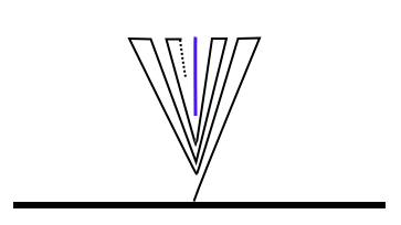
Figure 4. A curve $\gamma$ approaching a vertical line segment (blue).

Example 3.11.

Consider the simply connected domain $D=\mathbb{H}\setminus\overline{\mathbb{D}}$. Let $F_{\mu}:\mathbb{H}\to D$ be univalent. The density $d$ of $\mu$ is symmetric with respect to the homeomorphism $h(x)=-x$, but $\mathcal{H}_{\mu}(h(x))=-\mathcal{H}_{\mu}(x)$.

3.2. Cauchy transforms vs Fourier transforms

The Fourier transform of a probability measure $\mu$ is given as $\mathcal{F}_{\mu}(x)=\int_{\mathbb{R}}e^{ixt}\mu(dt)$, $x\in\mathbb{R}$. Classical independence of random variables leads to the classical convolution $\mu\ast\nu$ defined by

$$\mathcal{F}_{\mu\ast\nu}=\mathcal{F}_{\mu}\cdot\mathcal{F}_{\nu}.$$

Definition 3.12.

A stochastic process $(X_{t})_{t\geq 0}$ is called an additive process if the following three conditions are satisfied.

1. The increments $X_{t_{0}},X_{t_{1}}-X_{t_{0}},...,X_{t_{n}}-X_{t_{n-1}}$ are independent for any choice of $n\geq 1$ and $0\leq t_{0}<t_{1}<...<t_{n}$.

2. $X_{0}=0$ almost surely.

3. For any $\varepsilon>0$ and $s\geq 0$, $\mathbb{P}[|X_{s+t}-X_{s}|>\varepsilon]\to 0$ as $t\to 0$.

Such a process is called a Lévy process if, in addition,

1. the distribution of $X_{t+s}-X_{s}$ does not depend on $s$.

Definition 3.13.

A probability measure $\mu$ on $\mathbb{R}$ is said to be $\ast$-infinitely divisible if for every $n\in\mathbb{N}$ there exists $\mu_{n}$ such that $\mu=\mu_{n}\ast...\ast\mu_{n}$ ($n$-fold convolution). The set of all infinitely divisible distributions is denoted by ${\rm\bf ID}(\ast)$.

The following result characterizes all distributions appearing in additive processes, see [BNMR01, Theorems 1.1-1.3].

Theorem 3.14.

Let $\mu$ be a probability measure on $\mathbb{R}$. The following statements are equivalent:

1. There exists an additive process $(X_{t})_{t\geq 0}$ such that $\mu$ is the distribution of $X_{1}$.

2. There exists a Lévy process $(X_{t})_{t\geq 0}$ such that $\mu$ is the distribution of $X_{1}$.

3. $\mu\in{\rm\bf ID}(\ast)$.

4. (Lévy-Khintchine representation) There exist $a\in\mathbb{R}$, $\sigma\geq 0$, and a non-negative measure $\nu$ with $\nu(\{0\})=0$ and $\int_{\mathbb{R}}(1\wedge t^{2})\nu(dt)<\infty$ such that

   (3.1) $$\mathcal{F}_{\mu}(x)=\exp\left(iax-\frac{1}{2}\sigma^{2}x^{2}+\int_{\mathbb{R}}\left(e^{ixt}-1-ixt1_{\{|x|<1\}}\right)\nu(dt)\right),\qquad x\in\mathbb{R}.$$

Remark 3.15.

For $\mu\in{\rm\bf ID}(\ast)$, we denote by $L(\mu)=(a,\sigma,\nu)$ the Lévy triple of $\mu$. If we shift $\mu$ by a constant $c\in\mathbb{R}$, then we obtain $L(\mu(\cdot-c))=(a+c,\sigma,\nu)$.

The $F$-transform plays the role of the Fourier transform in monotone probability theory. The monotone convolution $\mu\rhd\nu$ is defined by

$$F_{\mu\rhd\nu}=F_{\mu}\circ F_{\nu}.$$

The monotone analogue of property (a) in Theorem 3.14 is the property of $F_{\mu}$ being a univalent function.

Theorem 3.16 (Theorem 1.16 in [FHS18]).

Let $\mu$ be a probability measure on $\mathbb{R}$. The following statements are equivalent:

• $F_{\mu}$ is univalent.

• There exists a quantum process $(X_{t})_{t\geq 0}$ with monotonically independent increments such that $\mu$ is the distribution of $X_{1}$.

For the precise meaning of the quantum process mentioned in (b), we refer the reader to [FHS18].

Remark 3.17.

Let $\mu_{t}$ be the distribution of $X_{t}$ and let $f_{t}=F_{\mu_{t}}$. In [FHS18, Proposition 3.11] it is shown that $(f_{t})$ is a decreasing Loewner chain, i.e. every $f_{t}$ is univalent and $f_{t}(\mathbb{H})\subset f_{s}(\mathbb{H})$ whenever $s\leq t$. In case $t\mapsto f_{t}$ is differentiable, it satisfies a Loewner equation of the form

$$\frac{\partial}{\partial t}f_{t}(z)=\frac{\partial}{\partial z}f_{t}(z)\cdot M(z,t),$$

where $M(z,t)=\gamma_{t}+\int_{\mathbb{R}}\frac{1+xz}{x-z}\rho_{t}({\rm d}x)$ for some $a_{t}\in\mathbb{R}$ and a finite non-negative measure $\rho_{t}$ on $\mathbb{R}$.

Let us compare this to classical additive processes:

Let $(\mu_{t})_{t\geq 0}$ be the distributions of a Lévy process and let $\mathcal{F}_{t}=\mathcal{F}_{\mu_{t}}$. Then $(\mathcal{F}_{t})_{t\geq 0}$ is a multiplicative semigroup with $\mathcal{F}_{1}(x)=\mathcal{F}_{\mu}(x)=e^{\varphi(x)}$, i.e. $\mathcal{F}_{t}=e^{t\varphi(x)}$ or

$$\frac{d}{dt}\mathcal{F}_{t}(x)=\varphi(x)\cdot\mathcal{F}_{t},\qquad\mathcal{F}_{0}(x)\equiv 1.$$

The non-autonomous case of this equation is given by

$$\frac{d}{dt}\mathcal{F}_{t}(x)=\varphi_{t}(x)\cdot\mathcal{F}_{t},\qquad\mathcal{F}_{0}(x)\equiv 1,$$

where $\exp(\varphi_{t}(x))=\mathcal{F}_{\nu_{t}}$ with $\nu_{t}\in{\rm\bf ID}(\ast)$ for almost every $t\geq 0$. This equation corresponds to additive processes, provided that $t\mapsto\mathcal{F}_{\mu_{t}}(x)$ is indeed differentiable almost everywhere.

By replacing the $F$-transform with the classical Fourier transform, we can ask some questions from Section 2 now for the Fourier transform.

Consider an additive process $(X_{t})$ with distributions $(\mu_{t})$. Let $(a_{t},\sigma_{t},\nu_{t})=L(\mu_{t})$. Then we can normalize the process by $Y_{t}=X_{t}-a_{t}$. Also $(Y_{t})$ is an additive process and the distributions $(\alpha_{t})$ of $(Y_{t})$ satisfy $L(\alpha_{t})=(0,\sigma_{t},\nu_{t})$. Let $\mu\in{\rm\bf ID}(\ast)$. Let $(X_{t})$ and $(Y_{t})$ be two normalized additive processes such that $\mu$ is the distribution of $X_{1}$ and of $Y_{1}$.
We say that $\mu$ has a unique embedding if the distributions of $(Y_{t})$ are obtained by a time change of the distributions of $(X_{t})$.

Theorem 3.18.

Let $\mu\in{\rm\bf ID}(\ast)$ with Lévy triple $L(\mu)=(0,\sigma,\nu)$.

• $\mu$ can be embedded into an additive process $(X_{t})$ with distributions $(\mu_{t})$ such that $t\mapsto\mathcal{F}_{\mu_{t}}$ is differentiable everywhere.

• $\mu$ has a unique embedding if and only if $\nu=0$ or $\sigma=0$ and $\nu=\lambda\delta_{x_{0}}$ for some $x_{0}\in\mathbb{R}\setminus\{0\}$.

Proof.

• Due to Theorem 3.14, each $\mu\in{\rm\bf ID}(\ast)$ can be embedded into a Lévy process.

• Let $\mu$ be embedded into a normalized process $(X_{t})$ with distributions $\mu_{t}$. Let $L(\mu_{t})=(0,\sigma_{t},\nu_{t})$. The Lévy-Itô decomposition yields two independent additive processes $(A_{t})$ and $(B_{t})$ with Lévy triples $(0,\sigma_{t},0)$ and $(0,0,\nu_{t})$ respectively such that $X_{t}=A_{t}+B_{t}$. We define the process $(Y_{t})_{t\in[0,1]}$ by $Y_{t}=A_{2t}$ for $t\in[0,1/2]$ and $Y_{t}=Y_{1/2}+B_{2(t-1/2)}$ for $t\in(1/2,1]$. Then $Y_{1}=A_{1}+B_{1}$ has the distribution $\mu$.
  Let $\mu$ have a unique embedding. Then $(Y_{t})$ is a time change of $(X_{t})$ and this implies that $\nu_{t}=0$ for all $t\geq 0$, and thus $L(\mu)=(0,\sigma,0)$, or $\sigma_{t}=0$ for all $t\geq 0$ and thus $L(\mu)=(0,0,\nu)$.
  Furthermore, suppose $L(\mu)=(0,0,\nu)$ with $\nu(\mathbb{R})>0$ and $\nu$ is not of the form $\lambda\delta_{x_{0}}$. Then the support of $\nu$ consists of at least two points and we can decompose $\nu$ into $\nu=\nu_{1}+\nu_{2}$ for some positive measures $\nu_{1},\nu_{2}$ having different supports. A similar construction shows that the unique embedding of $\mu$ implies $\nu_{1}=0$ or $\nu_{2}=0$, a contradiction.
  

  Conversely, assume that $\mu$ with $L(\mu)=(0,\sigma,0)$ (or $L(\mu)=(0,0,\lambda\delta_{x_{0}})$) is embedded into an additive process $(X_{t})$ with distributions $\mu_{t}$ such that $L(\mu_{s})=(0,\sigma_{s},\nu_{s})$ with $\nu_{s}\not=0$ (or $\sigma_{s}\not=0$) for some $s<1$. Then $\mu=\mu_{s}\ast\mu_{s,1}$, where $\mu_{s,1}$ is the distribution of $X_{1}-X_{s}$, and this implies that $L(\mu)=(0,\sigma,\nu)$ for some $\nu\not=0$ (or $\sigma\not=0$), a contradiction.
  Hence, $L(\mu_{t})=(0,\sigma_{t},0)$ (or $L(\mu_{t})=(0,0,\lambda_{t}\delta_{x_{0}})$) for all $t\in[0,1]$ and $t\mapsto\sigma_{t}$ (or $t\mapsto\lambda_{t}$) is non-decreasing. Such processes are unique with respect to time changes.

∎

Remark 3.19.

The cases from (b) correspond to the Dirac measure at $0$ ($\sigma=0,\nu=0$), the normal distribution with mean 0 and variance $\sigma^{2}$ ($\sigma>0,\nu=0$), and the case $\sigma=0,\nu=\lambda\delta_{x_{0}}\not=0$ corresponds to certain Poisson distributions. Let $N$ be a Poisson random variable with parameter $\lambda>0$ and let $X=x_{0}\cdot N$ for some $x_{0}\not=0$. The distribution $\mu$ of $X$ satisfies $\mathcal{F}_{\mu}(x)=\exp(\lambda(e^{ixx_{0}}-1))$. If $|x_{0}|\geq 1$, then $L(\mu)=(0,0,\lambda\delta_{x_{0}})$.
If $|x_{0}|<1$, then $L(\mu)=(\lambda x_{0},0,\lambda\delta_{x_{0}})$. Hence, the distribution of $X-\lambda x_{0}$ has the Lévy triple $(0,0,\lambda\delta_{x_{0}})$.
Our definition of a “normalized additive process” is somehow arbitrary, basically because the cut–off function in representation (3.1) can be replaced by others.
One could also normalize by subtracting the mean of $\mu$, provided it exists. However, also there, we end up with the Dirac measure at $0$, the normal distribution with mean $0$ and variance $\sigma^{2}$, and (scaled and shifted versions of) the Poisson distribution.

3.3. Problems

Problem 3.20.

Let $\mu$ be a probability measure satisfying the conditions $(a)$-$(c)$ from Theorem 3.3 or 3.5 respectively. Is $F_{\mu}$ necessarily univalent?

Problem 3.21.

Which probability measures $\mu$ have a surjective $F$-transform, i.e. $F_{\mu}(\mathbb{H})=\mathbb{H}$. An example of such $\mu$ is given in Remark 3.6.

Problem 3.22.

Motivated by Theorem 3.3, we can replace the Hilbert transform $\mathcal{H}_{\mu}$ by some other transform $T_{\mu}$ and consider probability measures $\mu$ such that there exists a decreasing homeomorphism $h:\mathbb{R}\to\mathbb{R}$ with

$$\mu(A)=\mu(h(A))\quad\text{and}\quad T_{\mu}\circ h=T_{\mu}$$

for all Borel sets $A\subset\mathbb{R}$.
Is it true that in case $T_{\mu}=\mathcal{F}_{\mu}$ we necessarily have $h(x)=-x$?
An example is the normal distribution with mean $0$ and variance $\sigma^{2}$, where $\mathcal{F}_{\mu}(x)=e^{-\sigma^{2}x^{2}/2}$, and thus $h(x)=-x$.

Acknowledgements

The authors would like to thank Mihai Iancu for helpful discussions and the proof of Theorem 2.2.

References

- [Ayr29] W. L. Ayres, On Simple Closed Curves and Open Curves, Proceedings of the National Academy of Sciences of the United States of America Vol. 15, No. 2 (1929), 94–96.
- [BNMR01] O. E. Barndorff-Nielsen, T. Mikosch, and S. I. Resnick, Lévy Processes, Theory and Applications, Birkhüaser, 2001.
- [Bis07] C. J. Bishop, Conformal welding and Koebe’s theorem, Annals of Mathematics, 166 (2007), 613–656.
- [Böh16] C. Böhm, Loewner equations in multiply connected domains, PhD dissertation, Würzburg, 2016.
- [CMR06] J. Cima, A. Matheson, and W. T. Ross, The Cauchy transform, Mathematical Surveys and Monographs, 125, American Mathematical Society, Providence, RI, 2006.
- [Dur83] P. L. Duren, Univalent functions, volume 259 of Grundlehren der Mathematischen Wissenschaften [Fundamental Principles of Mathematical Sciences], Springer-Verlag, New York, 1983.
- [Fia17] M. Fiacchi, The embedding conjecture and the approximation conjecture in higher dimension, arXiv:1710.02087.
- [FW18] J. E. Fornaess, E. Fornaess Wold, An embedding of the unit ball that does not embed into a Loewner chain, arXiv:1806.03591.
- [FHS18] U. Franz, T. Hasebe, and S. Schleißinger, Monotone Increment Processes, Classical Markov Processes and Loewner Chains, arXiv:1811.02873.
- [Hot] I. Hotta, Loewner theory for quasiconformal extensions: old and new, arXiv:1402.6006.
- [LLN09] S. Lalley, G. Lawler, and H. Narayanan, Geometric Interpretation of Half-Plane Capacity, Elect. Comm. in Probab. 14 (2009), 566–571.
- [Law05] G. F. Lawler, Conformally invariant processes in the plane, volume 114 of Mathematical Surveys and Monographs. American Mathematical Society, Providence, RI, 2005.
- [Lin05] J. R. Lind, A sharp condition for the Loewner equation to generate slits, Ann. Acad. Sci. Fenn. Math. 30(1) (2005), 143–158.
- [LR12] J. Lind and S. Rohde, Space–filling curves and phases of the Loewner equation, Indiana Univ. Math. J. 61 (2012), no. 6, 2231–2249.
- [Löw23] K. Löwner, Untersuchungen über schlichte konforme Abbildungen des Einheitskreises. I, Math. Ann. 89 (1923), no. 1-2, 103–121.
- [Maa92] H. Maassen, Addition of freely independent random variables, J.Funct. Anal. 106 (1992), no. 2, 409–438.
- [MR05] D. E. Marshall and S. Rohde, The Loewner differential equation and slit mappings, J. Amer. Math. Soc. 18(4) (2005), 763–778.
- [Pom66] C. Pommerenke, On the Loewner differential equation. Michigan Math. J. 13 (1966), 435–443.
- [Pom92] C. Pommerenke, Boundary behaviour of conformal maps. Grundlehren der Mathematischen Wissenschaften & Springer-Verlag, Berlin, 1992.
- [Pom75] C. Pommerenke, Univalent functions. Vandenhoeck & Ruprecht, Göttingen, 1975.
- [Sat99] K. Sato, Lévy Processes and Infinitely Divisible Distributions, Cambridge Studies in Advanced Mathematics, 1999.
- [Sch12] K. Schmüdgen, Unbounded self-adjoint operators on Hilbert space, Graduate Texts in Mathematics, Vol. 265, Springer, Dordrecht, 2012.
- [Wil63] R. L. Wilder, Topology of manifolds, Reprint of 1963 edition. American Mathematical Society Colloquium Publications, 32. American Mathematical Society, Providence, R.I..
- [ZZ18] H. Zhang and M. Zinsmeister, Local Analysis of Loewner Equation, arXiv:1804.03410.