Thermal fluctuations and dynamic modelling of a dAFM cantilever

Abstract

We discuss the Brownian thermal noise which affects the cantilever dynamics of a dAFM (dynamic atomic force microscope), both when it works in air and in presence of water. Our scope is to accurately describe the cantilever dynamics, and to get this result we deeply investigate the relationship between the cantilever thermal fluctuations and its interactions with the surrounding liquid. We present a relatively simple and very easy-to-use analytical model to describe the interaction forces between the liquid and the cantilever. The novelty of this approach is that, under the assumption of small cantilever oscillations, by using the superposition principle we found a very simple integral expression to describe fluid-cantilever interactions. More specifically we note that, beside including fluid inertia and viscosity (which is common to many existing models in the literature) an additional diffisivity term needs to be considered, whose crucial influence for the correct evaluation of the cantilever response to the thermal excitation is shown in the present paper. The coefficients of our model are obtained by using numerical results for a 2D fluid flow around a vibrating rectangular cross-section, and depend on the distance from the wall. This allowed us to completely characterize the dynamics of a dAFM cantilever also when it operates in tilted conditions. We validate the analytical model by comparing our results with numerical and experimental dAFM data previously presented in literature, and with experiments carried out by ourselves. We show that we can provide extremely accurate prediction of the beam response up and beyond the second resonant peak.

Part I Introduction

The dynamic atomic force microscope (dAFM) consists of an oscillating microcantilever which holds a sharp nanoscale tip that intermittently interacts with the sample, close to its first resonance frequency. There are many fields of applications of dAFM, and ranges from measuring topography of organic and inorganic materials at nanometer length scales, to the accurate quantification of sample properties in materials science. Despite many years of investigations on dAFM dynamics 1 , several aspects still demand further attention from the research community. Because of the complexity related to the small scales involved, where different physical effects coexist together, it is a very common approach to study each phenomenon separately, and to draw conclusions from each analysis 2 ; 3 . This is often a very good way to clarify aspects completely unknown before, but for more detailed insights, it is also necessary to analyze different effects together. This is the case of the dAFM research field, in which, in particular, it is extremely important to analyse both the tip-sample and the fluid-structure interactions. For such instruments a clear signal is one of the utmost requirements in order to extract correct information from the measurement at so small length scales. However this is not a so straightforward task to be achieved because of the forces which act on the cantilever in operational conditions, especially when a liquid environment is required, e.g. in physiological buffer solutions 4 ; 5 ; 6 ; 7 . In such case, in particular, besides the tip-sample interaction, the presence of a liquid deeply modifies the response spectrum and is the origin of the so called Brownian thermal noise. Indeed, even though the molecular size of the fluid molecules is negligibly small in comparison to the size of the cantilever, the dynamics of the cantilever itself is strongly dependent on Brownian fluctuations, since the same molecular processes are responsible for both the dissipation and the fluctuations, due to the collisions between the fluid molecules and the cantilever. But to achieve a good AFM resolution, noise sources must be reduced as much as possible, since the lowest signal level that can be considered as a valid information must be not mixed up with external noise. In spite of this, the cantilever thermal motion is also utilized to calibrate the cantilever’s spring constant 8 and to extract the resonance frequencies and quality factors of its resonances as well 9 . Therefore, a good understanding and theoretical modelling of this effect related to the equilibrium of the cantilever with the surrounding liquid is of paramount importance, whatever is the scope, i.e. either to study ad hoc control system to separate the signal from noise, or to obtain useful insights about the cantilever properties. With such an aim, several studies have been presented up to now 10 ; 11 ; 12 , but the main difficulty for a proper description of the cantilever response to the thermal fluctuations is the fluid-structure interaction modelling. In order to overcome the complexity of the problem, some assumptions have been made in the previous studies, such as those of neglecting inertia 13 and the diffusivity 14 ; 15 ; Paul2006 ; Cole2007 terms, which, instead, become important from intermediate to high frequency range. In this paper the authors present an analytical model to describe the drag of the liquid on the cantilever which takes into account, in a relatively simple way, all the three mentioned contributions: (i) the fluid viscosity, (ii) fluid inertia, and (iii) the fluid vorticity diffusivity. It is shown, in particular, that the correct evaluation of the cantilever response to the thermal excitation cannot neglect the above mentioned effects. Moreover, experimental results of an AFM cantilever working in air are presented, which definitively assess the accuracy of the model.

The paper is organized as follows: in Sec.I, the model used to describe the cantilever dynamics is presented; in Sec.II the new general expression of the liquid drag is heuristically derived; in Sec.III the relation between the cantilever response and the Brownian loading spectra is shown; in Sec. IV our analytical model is compared with previous works and with our experimental results; in Sec. V we provide concluding remarks; in Appendix A we show how to calculate the susceptibility function of the cantilever; in Appendix B the Fluctuation Dissipation Theorem for a 1DOF system is shown; in Appendix C we analytically derive the Fluctuation Dissipation Theorem for the continuous system we are studying, i.e. for the cantilever; in Appendix D the Equiripartition theorem for the cantilever case is derived.

I Cantilever dynamics

We study the dynamics of a cantilever immersed in a viscous fluid (see Figure 1) near a rigid flat wall, with $L$, $B$, and $H$ respectively the length, the width and the thickness of the rectangular cross section. We will assume that $L\gg B\gg H$, as well as that the transversal displacement $\left|w\left(x,t\right)\right|\ll L$. This enables us to use the Bernoulli theory of transversal vibrations and therefore neglect the influence of shear stress in the beam. The general motion equation of the cantilever is therefore:

Figure 1: dAFM microcantilever.

$$EI\frac{\partial^{4}w\left(x,t\right)}{\partial x^{4}}+\rho A\frac{\partial^{2}w\left(x,t\right)}{\partial t^{2}}=f_{B}\left(x,t\right)+f_{L}\left(x,t\right)$$ (1)

where $\rho$ is the bulk density of the material the cantilever is made of, $E$ is the Young’modulus and $A$ is the area of the cross section of the beam, i.e. $A=BH$. In the RHS of the above Eq. (1) we have introduced two terms. The first term $f_{B}\left(x,t\right)$ is the chaotic force per unit length acting on the beam as a consequence of the thermal fluctuation of the molecules constituting the liquid: we will refer to this type of excitation term as the Brownian force.

The term $f_{L}\left(x,t\right)$ is the force per unit length which the liquid, in a continuum sense, exerts on the cantilever, which is usually calculated by means of complex numerical simulations. However, under the hypothesis of small transversal displacements $\left|w\left(x,t\right)\right|\ll B$, we can assume that the response of the fluid is linear. Under this condition the force $f_{L}\left(x,t\right)$ can be expressed in terms of the response function $G\left(x,x^{\prime},t\right)$:

$$f_{L}\left(x,t\right)=\int_{-\infty}^{t}d\tau\int_{0}^{L}dx^{\prime}G\left(x,x^{\prime},t-\tau\right)\frac{\partial v\left(x^{\prime},\tau\right)}{\partial\tau}$$ (2)

where $v\left(x,\tau\right)$ is the transversal velocity of the generic cantilever section, i.e. $v\left(x,\tau\right)=w_{t}\left(x,t\right)$ , where the subscript $t$ denotes the partial time-derivative. Moreover, causality implies the linear response function of the liquid must vanish for $t<0$. This also implies that the quantity

$$G\left(x,x^{\prime},\omega\right)=\int_{-\infty}^{+\infty}dtG\left(x,x^{\prime},t\right)\exp\left(-i\omega t\right)$$ (3)

must be analytic in lower half-plane of the complex domain, and therefore must satisfy the Kramer-Kronig relations 20 . However, measurements or numerical calculations contain always some errors or approximations that do not guarantee the Kramer-Kroning relations to be exactly satisfied. This restriction in general leads to some difficulties in the calculations of the linear response function $G\left(x,x^{\prime},t\right)$ of the liquid from the measured or numerically calculated frequency response, i.e. it is often not possible to determine the quantity $G\left(x,x^{\prime},t\right)$ by simply taking the inverse Fourier transform of the measured frequency response of the system. However the task is much more simplified if the analytical form of this function is already known. For this reason, the authors have derived a new analytical model of the liquid response $G\left(x,x^{\prime},t\right)$, that will be presented in the next section.

II Fluid-cantilever interaction

We first observe that some hypothesis about the time dependence of the liquid response function $G\left(t\right)$ must be fulfilled. Indeed, the assumption that $L\gg B\gg H$ allows us to consider that the response of the fluid depends only on local quantities, i.e. the fluid motion is locally two dimensional 13 ; 15 . In such case we can write $G\left(x,x^{\prime},t\right)=G\left(x,t\right)\delta\left(x^{\prime}-x\right)$. Now, the leading-order incompressible flow generated by an isolated body oscillating at small amplitude is governed by the unsteady Stokes equation

$$\rho_{L}\frac{\partial\mathbf{v}}{\partial t}+\rho_{L}\left(\mathbf{v}\cdot\nabla\right)\mathbf{v} =-\nabla p+\eta\nabla^{2}\mathbf{v}$$ (4)

$$\nabla\cdot\mathbf{v} =0$$

where $\mathbf{v}$ is the velocity of the fluid, $\eta$ is the liquid viscosity, $\rho_{L}$ the liquid density. Observe that the non-linear term $\rho_{L}\left(\mathbf{v}\cdot\nabla\right)\mathbf{v}$ can be neglected in comparison with the time derivative of Eq.4. Indeed, by estimating the two terms, we obtain that $\rho_{L}\left(\mathbf{v}\cdot\nabla\right)\mathbf{v\sim}\left(w_{0}\omega\right)^{2}/B$, and the time derivative $\rho_{L}\partial\mathbf{v/}\partial t\mathbf{\sim}w_{0}\omega^{2}$, being $B$ the characteristic dimensions of the moving bodies, i.e. the width of the cantilever cross section, and $w_{0}$ the amplitude of the oscillations. Therefore the non linear convective term can be neglected if $w_{0}\ll B$, which is indeed one of the hypotheses of our model. Moreover, Eq. (4) can be rephrased in terms of the vorticity $\mathbf{W}\mathbf{=}\nabla\times\mathbf{v}$ as $\rho_{L}\left(\partial\mathbf{W/}\partial t\right)=\eta\nabla^{2}\mathbf{W}$, showing that the vorticity is governed by a diffusive-like equation which generates an exponential decay of the velocity as we move far from the walls of the bodies towards the interior of the liquid. The exponential decay allows to estimate the thickness $h$ of the layer of fluid within which the flow is rotational and velocity diffusion is important. It is known 16 that $h\sim\omega^{-1/2}$ where $\omega$ is the characteristic frequency of the motion. Out of the layer the term $\nabla^{2}\mathbf{v}$ can be neglected in Eq. 4 so that we have potential flow. Since the value of $h$ depends on the frequency $\omega$, it follows that at large frequencies the thickness $h$ will be very small and the response of the fluid will be then governed by inertia effects, i.e. it will depend proportionally on the acceleration $v_{t}\left(x,t\right)$ of the moving bodies. In this limiting case $G\left(x,t\right)=-\mu\left(x\right)\delta\left(t\right)$, where $\delta\left(t\right)$ is the Dirac delta function. If, on the contrary, the motion is sufficiently slow (low $\omega$-values) then the term $\partial\mathbf{v/}\partial t$ can be neglected and the quantity $h$ becomes larger than the characteristic dimensions of the moving bodies. The motion of the fluid becomes steady and the response of the fluid should depend linearly on the velocity $v$ of the moving bodies, i.e. for $t\geq 0$, we have $G\left(x,t\right)=-c\left(x\right)$. At intermediate frequency the effect of diffusivity should be very important. It is known 16 that for the in-plane motion of flat plate the motion of the liquid is governed by a pure diffusive equation, and in this case $G\left(x,t\right)$ takes the form $G\left(x,t\right)=-\alpha\left(x\right)t^{-1/2}$ for $t\geq 0$, which represents the contribution to the fluid force coming from the diffusion of the tangential velocity of the plate into the interior of the liquid. Since Eqs. (4) are linear, the force the liquid exerts on the body will be given by the sum of the three contributions and we can heuristically give a general expression for $G\left(x,t\right)$ as

$$G\left(x,t\right) =-c\left(x\right)-\frac{\alpha\left(x\right)}{\sqrt{t}}-\mu\left(x\right)\delta\left(t\right);\qquad t\geq 0$$ (5)

$$G\left(x,t\right) =0;\qquad t<0$$

where $c\left(x\right)$ is the damping, $\alpha\left(x\right)$ is the diffusive coefficient, and $\mu\left(x\right)$ is the inertia term. Eq.(5), therefore, satisfies the causality principle. We observe, in particular, that for the case of a sphere moving in a liquid, the response of the fluid has exactly the form given by Eq. (5), see for example 16 . Moreover, by substituting Eq.(5) and Eq.(2) in Eq.(1), we get

$$EI\frac{\partial^{4}w\left(x,t\right)}{\partial x^{4}}+\left[\rho A+\mu\left(x\right)\right]\frac{\partial^{2}w\left(x,t\right)}{\partial t^{2}}+c\left(x\right)\frac{\partial w\left(x,t\right)}{\partial t}+$$ (6)

$$+\alpha\left(x\right)\int_{-\infty}^{t}d\tau\frac{1}{\sqrt{t-\tau}}\frac{\partial^{2}w\left(x,\tau\right)}{\partial\tau^{2}} =f_{B}\left(x,t\right)$$

and in particular, the linear response function $\chi\left(x,x^{\prime},t\right)$ of this equation, also referred to as susceptibility, can be obtained by solving the fundamental problem (see Appendix A):

$$EI\frac{\partial^{4}\chi\left(x,x^{\prime},t\right)}{\partial x^{4}}+\left[\rho A+\mu\left(x\right)\right]\frac{\partial^{2}\chi\left(x,x^{\prime},t\right)}{\partial t^{2}}+c\left(x\right)\frac{\partial\chi\left(x,x^{\prime},t\right)}{\partial t}+$$ (7)

$$+\alpha\left(x\right)\int_{-\infty}^{t}d\tau\frac{1}{\sqrt{t-\tau}}\frac{\partial^{2}\chi\left(x,\tau\right)}{\partial\tau^{2}} =\delta\left(x-x^{\prime}\right)\delta\left(t\right)$$

Eq. (5) is, of course, approximated, but in what follows it will be shown that it works very well. In Eq. (5) the $x$-dependence can be present only as a consequence of the $x$- dependent distance of the cantilever cross sections from the wall, i.e. only when the beam is tilted, which is a case also covered by this study. Once the analytical form of the response function is known, the three coefficients can be determined by finding the best fitting with the existing accurate computational fluid dynamics non-dimensional solutions of a 2D fluid flowing around a vibrating rectangular cross-section, as reported in Ref. 15 . In Table1, the three coefficients are shown, calculated in correspondence of the cantilever free end $x=L$, for different values of $\Delta=2d/B$, where $d$ is the wall distance. Now, Fourier transforming Eq. (6) we obtain

$$\frac{\partial^{4}w\left(x,\omega\right)}{\partial x^{4}}-B\left(x,\omega\right)^{4}w\left(x,\omega\right)=f_{B}\left(x,\omega\right)$$ (8)

where we define the function $B\left(x,\omega\right)$

$$B\left(x,\omega\right)=\sqrt[4]{-\frac{i\omega c\left(x\right)-\left[\rho A+\mu\right]\omega^{2}+i\omega~{}\alpha\left(x\right)\sqrt{i\omega\pi}}{EI}}$$ (9)

$\Delta$	$c\ \mathrm{[kg\ s}^{-1}\mathrm{]}$	$\alpha\ \mathrm{[kg\ s}^{-1/2}\mathrm{]}$	$\mu\ \mathrm{[kg]}$
$0.5$	$0.157$	$8.32\times 10^{-6}$	$5.73\times 10^{-7}$
$1$	$0.042$	$1.25\times 10^{-5}$	$4.65\times 10^{-7}$
$2$	$0.016$	$2.13\times 10^{-5}$	$4.13\times 10^{-7}$
$4$	$8.6\times 10^{-3}$	$3.72\times 10^{-5}$	$3.81\times 10^{-7}$
$6$	$6.05\times 10^{-3}$	$4.91\times 10^{-5}$	$3.65\times 10^{-7}$
$8$	$4.91\times 10^{-3}$	$5.65\times 10^{-5}$	$3.56\times 10^{-7}$
$10$	$4.31\times 10^{-3}$	$6.1\times 10^{-5}$	$3.51\times 10^{-7}$

Tab.1 - The three coefficients of the fluid response, at the free end of the cantilever $x=L$, for different values of the distance $\Delta=2d/B$ of the cantilever from the substrate.

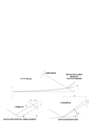
Figure 2: The total displacement $w_{tot}$ of the laser beam on the photodiode is given by the weighted sum of both the vertical displacement $s\left(x,t\right)$ and the rotation $\gamma\left(x,t\right)$ of the cantilever.

III The fluctuation dissipation theorem

In AFM systems the micrometer size of the cantilever makes it particularly sensitive to Brownian fluctuations so that the thermal induced fluctuations of the cantilever displacement cannot be neglected, thus making the measurement of the response function of the cantilever through its thermal fluctuations a viable technique. This is done by employing the Fluctuation Dissipation Theorem (FDT) (see Appendix B). The FDT states that the susceptibility function $\chi\left(x_{1},x_{2},t\right)$ of the cantilever, which is the displacement $w\left(x_{1},\omega\right)$ at point $x_{1}$ due to the action of a concentrated unit force $F$ at point $x_{2}$, is proportional to the time-derivative of the correlation function of the thermal fluctuations of the cantilever displacements (see Appendix C) 17 , that is

$$\chi\left(x_{1},x_{2},t\right)=-\beta H\left(t\right)\frac{\partial}{\partial t}\left\langle w\left(x_{1},0\right)w\left(x_{2},t\right)\right\rangle$$ (10)

where $\beta=\left(k_{B}T\right)^{-1}$ and $k_{B}$ is Boltzmann’s constant, $T$ the absolute temperature and $H\left(t\right)$ is the Heaviside unit step function. The susceptibility function can be used to rephrase the solution of Eq. (1) as

$$w\left(x_{1},t\right)=\int_{-\infty}^{t}d\tau\int_{0}^{L}dx_{2}\chi\left(x_{1},x_{2},t-\tau\right)f_{B}\left(x_{2},\tau\right)$$ (11)

Moving from Eq.(10), the relation between the Cross Power Spectral Density (CPSD) $R\left(x_{1},x_{2},\omega\right)=\int dt~{}\left\langle w\left(x_{1},0\right)w\left(x_{2},t\right)\right\rangle\exp\left(-i\omega t\right)$ of the cantilever thermal fluctuations and the imaginary part of the time-Fourier transform of the susceptibility function, i.e. the imaginary part of the complex compliance $\chi\left(x_{1},x_{2},\omega\right)=\int dt\chi\left(x_{1},x_{2},t\right)\exp\left(-i\omega t\right)$, can be easily derived (see Appendix C) 18 as

$$R\left(x_{1},x_{2},\omega\right)=-\frac{2k_{B}T}{\omega}\operatorname{Im}\chi\left(x_{1},x_{2},\omega\right)$$ (12)

Eq. (12) will be used to calculate the PSD of the thermal oscillations of the free end of the cantilever. We observe that the CPSD $R\left(x_{1},x_{2},\omega\right)$ is, in general, not $\omega$-independent (as it should be in case of white noise), since, as we show later, the velocity-diffusive and the inertia terms of the liquid response, do not make $\operatorname{Im}[\chi\left(x_{1},x_{2},\omega\right)]$ proportional to the radian frequency $\omega$. Equation (12) shows that, in order to calculate the CPSD of the cantilever displacement fields, it is enough to measure or calculate the response function $\chi\left(x_{1},x_{2},\omega\right)$. However, this quantity is strongly affected by the presence of the liquid. By solving Eq. (8) it is possible to determine the complex compliance of the cantilever for the transversal displacement and therefore determine the CPSD $R\left(x_{1},x_{2},\omega\right)$. In order to define the correct signal information which is actually read by the AFM system, we point out that the angular rotation of the beam cross section gives a huge contribution to signal read by the photodiode. In Fig. 2, indeed, one can clearly observe that the total displacement $w_{\mathrm{tot}}\left(t\right)$ of the reflected laser spot on the photodiode surface can be calculated as the weighted sum of both the vertical $s\left(x,t\right)=w\left(x,t\right)$ displacement and the angular $\gamma\left(x,t\right)=\dot{s}\left(x,t\right)=$ $\left(\partial w/\partial x\right)_{l,t}$ rotation of the cantilever, i.e.

$$w_{\mathrm{tot}}\left(x,t\right)=c_{1}s\left(x,t\right)+c_{2}\gamma\left(x,t\right)$$ (13)

Therefore we will assume in what follows that the CPSD of the quantity $w_{\mathrm{tot}}\left(x,t\right)$ is $S_{\mathrm{tot}}\left(x_{1},x_{2},\omega\right)=\int dt\left\langle w_{\mathrm{tot}}\left(x_{1},0\right)w_{\mathrm{tot}}\left(x_{2},t\right)\right\rangle\exp\left(-i\omega t\right)$. So we get, at the cantilever free end $x_{1}=x_{2}=L$

$$\left\langle w_{\mathrm{tot}}\left(L,0\right)w_{\mathrm{tot}}\left(L,t\right)\right\rangle =c_{1}^{2}\ \left\langle w\left(L,0\right)w\left(L,t\right)\right\rangle+$$ (14)

$$+c_{1}c_{2}\left[\left\langle w_{x}\left(L,0\right)w\left(L,t\right)\right\rangle+\left\langle w\left(L,0\right)w_{x}\left(L,t\right)\right\rangle\right]+c_{2}^{2}\left\langle w_{x}\left(L,0\right)w_{x}\left(L,t\right)\right\rangle$$

Now recall that

$$\int dt\left\langle w\left(L,0\right)w\left(L,t\right)\right\rangle e^{-i\omega t}=R\left(L,L,\omega\right)=-\frac{2k_{B}T}{\omega}\operatorname{Im}\chi\left(L,L,\omega\right)$$ (15)

so taking the derivative we also obtain

$$\int dt\left\langle w_{x}\left(L,0\right)w\left(L,t\right)\right\rangle e^{-i\omega t} =R_{1}\left(L,L,\omega\right)=-\frac{2k_{B}T}{\omega}\operatorname{Im}\chi_{1}\left(L,L,\omega\right)$$ (16)

$$\int dt\left\langle w\left(L,0\right)w_{x}\left(L,t\right)\right\rangle e^{-i\omega t} =R_{2}\left(L,L,\omega\right)=-\frac{2k_{B}T}{\omega}\operatorname{Im}\chi_{2}\left(L,L,\omega\right)$$

$$\int dt\left\langle w_{x}\left(L,0\right)w_{x}\left(L,t\right)\right\rangle e^{-i\omega t} =R_{12}\left(L,L,\omega\right)=-\frac{2k_{B}T}{\omega}\operatorname{Im}\chi_{12}\left(L,L,\omega\right)$$

where $\left(\cdot\right)_{i}=\partial\left(\cdot\right)/\partial x_{i}$ and $\left(\cdot\right)_{ij}=\partial^{2}\left(\cdot\right)/\partial x_{i}\partial x_{j}$. The power spectrum of the signal recorded by the photodiode is then

$$S\left(\omega\right) =S_{\mathrm{tot}}\left(L,L,\omega\right)=\int dt\left\langle w_{\mathrm{tot}}\left(L,0\right)w_{\mathrm{tot}}\left(L,t\right)\right\rangle\exp\left(-i\omega t\right)$$

$$=c_{1}^{2}R\left(L,L,\omega\right)+c_{1}c_{2}\left[R_{1}\left(L,L,\omega\right)+R_{2}\left(L,L,\omega\right)\right]+c_{2}^{2}R_{12}\left(L,L,\omega\right)$$ (17)

$$=-\frac{2k_{B}T}{\omega}\operatorname{Im}\left\{c_{1}^{2}\chi\left(L,L,\omega\right)+c_{1}c_{2}\left[\chi_{1}\left(L,L,\omega\right)+\chi_{2}\left(L,L,\omega\right)\right]+c_{2}^{2}\chi_{12}\left(L,L,\omega\right)\right\}$$

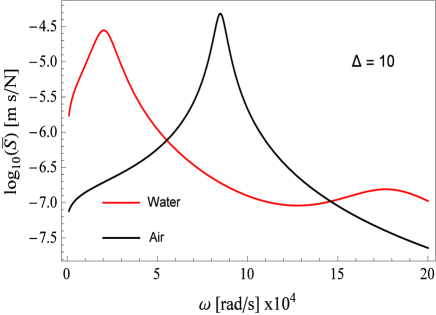
Figure 3: The cantilever thermal power spectrum in water (red curve) and in air (black curve), $\Delta=2d/B=10.$

IV Results

In this section we discuss the main results of our investigation. We compare the thermal response of the cantilever tip in air and in water, show how important is the influence of the diffusive-velocity term related to the parameter $\alpha\left(x\right)$, and also discuss the influence of the distance between the cantilever and the underlying substrate. The geometrical and mechanical properties of the cantilever, we have investigated, are listed in Tab.2. At first, we will focus on the PSD of the transversal displacement of the free end of the cantilever, i.e. we will focus on the quantity $S\left(\omega\right)=S\left(x_{1}=L,x_{2}=L,\omega\right)$.

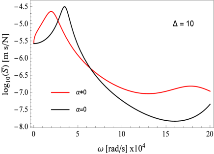
Figure 4: The influence of the velocity-diffusive term on the cantilever thermal power spectrum, for $\Delta=2d/B=10$.

Quantity	Value
$L$	$232.4~{}\mathrm{\mu m}$
$B$	$20.11~{}\mathrm{\mu m}$
$H$	$0.573~{}\mathrm{\mu m}$
Young Modulus	$3.92\times 10^{11}~{}\mathrm{Pa}$
Air density	$1.2~{}\mathrm{kg/m}^{3}$
Air -dynamic viscosity	$1.83\times 10^{-5}~{}\mathrm{Pas}$
Water density	$1000~{}\mathrm{kg/m}^{3}$
Water-dynamic viscosity	$1.0\times 10^{-3}~{}\mathrm{Pas}$

Tab.2 - The geometrical and physical quantities utilized to carry out the analysis.

Figure 3 shows the PSD of the cantilever tip deflection $\bar{S}\left(\omega\right)=S\left(\omega\right)/2k_{B}T$, when the dimensionless distance $\Delta=2d/B$ of the cantilever from the substrate is constant and equal to $\Delta=10$ ($d$ is the distance in $\mu m$), for a cantilever thermally excited in water (red curve) and in air (black curve). Observe the large peak shifting towards the low frequency range when the system is in water. At a first sight one may be surprised to see that the heights of the two peaks for water and air are not significantly different. However this can be easily explained considering that, although the imaginary part of the complex compliance is larger in air if compared to water, the peak frequency is about 3 times larger in air than in water. Hence, these two opposite effects partially balance each-other when the quantity $\bar{S}\left(\omega\right)$ is calculated. Beside this, one should also consider that, even in air, the presence of the wall makes non negligible the viscous dissipation related to the term $c\left(x\right)$ in Eq.5. Thus, a blunted resonant peak is expected to be observed as indeed shown in Fig. 3.

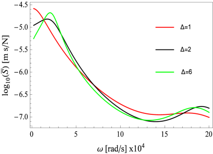
Figure 5: The thermal power spectrum for different values of the dimensionless distance $\Delta=2d/B$.

In Fig.4, the thermal power spectrum $\bar{S}\left(\omega\right)$ is shown, for $\alpha\neq 0$ as results from numerical fitting, and for $\alpha=0$. Fig. 4 shows the very large influence of the velocity-diffusive parameter in terms of peak resonance position and the Q-factor values. This means that neglecting such effect can lead to a strong overestimation of the first resonance frequency and also to strongly underestimate the noise affecting the dAFM at larger frequencies. This error in the evaluation of the cantilever thermal response to Brownian forcing, can in turn lead to a wrong calibration of the instrument. In particular, a bad estimation of the cantilever resonances and damping properties, yields an invalid estimation of the system properties and therefore may result in a non-correct operation of the instrument. This means that our drag model can be an extremely useful tool in the calibration process of a dAFM.

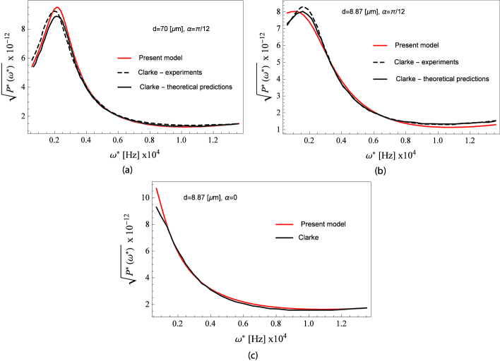
Figure 6: The thermal power spectrum $\sqrt{P^{\ast}\left(\omega^{\ast}\right)}$ in water near a wall. Comparison between experiments (dashed black curve) and theoretical predictions (solid black curve) presented in Ref.14 with our analytical model (solid red curve) for a tilt angle $\pi/12$ to the wall and separations $d=70\mu m$ (a) and $d=8.87\mu m$ (b). Theoretical predictions from Ref.14 (solid black curve) are also compared with our analytical model (solid red curve) for a tilt $\alpha=0$ and separation $d=8.87\mu m$ (c).

In Fig. 5 the cantilever thermal power spectrum $\bar{S}\left(\omega\right)$ at different distances from the substrate is shown. Three beam-wall distances are considered. The figure shows that the closer the cantilever is to the wall, the more the spectrum is shifted toward lower frequencies, whereas the second resonance peak occurs at higher frequencies. In particular, for the lowest value of $\Delta$ here considered, i.e. $\Delta=1$, the first resonant peaks almost disappears. The reason for such a strong influence of the substrate distance should be sought in the change of the viscous response of the liquid. Indeed at small beam-wall distances the viscous coefficient $c$ increases with $d^{-3}$ as the distance $d$ is reduced.

Considering that in many applications the cantilever is slightly tilted along its length, the effect of the $x$-dependent distance of the beam cross section from the substrate should be accurately taken into account to correctly estimate the cantilever response. This is the case of the experimental data shown in Ref.14 , where a cantilever in water is moved close to the substrate, with a tilt $\alpha=\pi/12$ (geometrical and physical quantities are the same listed in Table 2), and the angular oscillations are measured. In order to compare our analytical model with the numerical and experimental thermal power spectra presented in 14 , we have numerically calculated the interpolating functions of the three coefficients of the function $G\left(x,t\right)$ (Eq.5), i.e. $c\left(x\right)$, $m\left(x\right)$, and $\alpha\left(x\right)$, by means of the values reported in Table 1. Then we have calculated the PSD $S\left(\omega\right)$ (see Eq.17) given by both the vertical displacement and the angular rotation of the cantilever free end, and finally we have defined $P^{\ast}\left(\omega^{\ast}\right)=\left(\bar{A}^{2}/\omega_{0}\right)S\left(\omega\right)$, where $\bar{A}=\sqrt{k_{B}TL^{3}/\left(EJ\right)}$, $\omega^{\ast}=\omega_{0}\omega$, and $\omega_{0}=\sqrt{EJ/\left(\rho AL^{4}\right)}$. In Figure 6 we show the comparison of the quantity $\sqrt{P^{\ast}\left(\omega^{\ast}\right)}$ calculated by employing our analytical model (with $c_{1}=0$ and $c_{2}=0.86$ in Eq.17) and the experimental data and theoretical predictions presented in 14 , conducted in water, using a molecular force probe with pyramidal tip. In Fig.6-a the cantilever is tilted at $\pi/12$ to the wall with a separation $d=70\mu m$, in Fig.6-b the distance is reduced to $d=8.87\mu m$ (same tilt), in Fig. 6-c the cantilever has no tilt ($\alpha=0$) and the separation is $d=8.87\mu m$. In this last case no experimental data are presented in Ref. 14 and we show the comparison between our analytical model and the one utilized in 14 , where the fluid - cantilever interaction is described considering the Stokes’ expression for the drag on an oscillating circular cylinder. It is possible to observe a good agreement between our results (solid red lines), the experimental data (dashed black lines) and theoretical predictions (solid black lines) reported Ref.14 . It is worth of being mentioned that our analytical model is able to fit very well the experimental data (see Fig. 6-a). When the tilted cantilever is much closer to the wall (i.e. for $\Delta<1$) we expect to have a smaller degree of agreement, confirmed in Fig. 6-b, for the data presented in literature showed results for only a couple values of $\Delta$. In particular, considering the near wall case, we have found data only for $\Delta=0.5,1$ (see Table 1) that are not sufficient for an accurate estimation of the damping coefficient $c$.

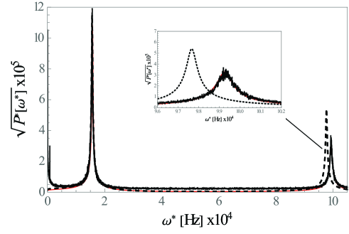
Figure 7: Our experimental thermal power spectrum $\sqrt{P^{\ast}\left(\omega^{\ast}\right)}$ in air (solid black curve), far from the wall, compared with our theoretical predictions (solid red curve) and the theoretical results presented in Ref.14 (dashed black curve). Our analytical model perfectly fit the experimental curve, also at the second resonant peak, as shown in the inset.

To completely assess our analytical model, we have carried out experiments with an AFM NT-MDT Ntegra Aura (Tribolab, Politecnico di Bari, Bari, Italy) on a CSG01 rectangular silicon cantilever with tip, and dimensions $\left(L,B,H\right)=\left(350,30,1\right)\mathrm{\mu m}$. The thermal oscillations of the free-end of the cantilever have been acquired, in the frequency range $0<\omega^{\ast}<105~{}\mathrm{kHz}$, where the first and the second resonant peaks of the beam are present. In Figure 7 our experimentally measured thermal power spectrum$\sqrt{P^{\ast}\left(\omega^{\ast}\right)}$ is compared with our theoretically predicted response. An almost perfect agreement between the experimental data and our theoretical model is obtained. The inset shows, in particular, that this almost perfect matching still holds true for the second resonant peak, a condition not easy achievable with other techniques (see dashed black curve in Fig.7 corresponding to the model reported in Ref.14 ). Our results definitively show that the presented analytical model is able to accurately predict the dynamics of a dAFM cantilever in a wide frequency range, thus making it a possible tool for calibration procedures and high performance measurements.

V Conclusions

The present study is concerned with the dAFM cantilever dynamics. More specifically, the attention has been focused on the interactions of the cantilever with the surrounding fluid. The impacts of the fluid molecules on the beam, indeed, generate the so called Brownian thermal noise, which is related to the macroscopic linear response of the system. An analytical model of the fluid-structure interactions has been presented, which takes into account of inertial, damping, and diffusive terms. In particular, the force the liquid exerts on the body has been heuristically derived, and it is described as the sum of three contributions, which have been evaluated through the best fitting of accurate computational fluid dynamics (adimensionalized) data of a 2D fluid flowing around an oscillating rectangular cross section, found in the literature. Experiments have been also carried out, and the thermal oscillations of a dAFM cantilever operating in air have been acquired. The experimental data have been perfectly fitted by means of our analytic response of the beam, in a wide frequency range. The results presented in this paper clearly demonstrate that our analytical model is an extremely useful and accurate tool to predict the cantilever dynamics, and therefore could be utilized to calculate the cantilever spring constants in the common calibration procedures, thus improving the quality of the measurements.

A. The Susceptibility Function

Here we calculate the complex compliance $\chi\left(x_{1},x_{2},\omega\right)$, which is the solution of the motion equation

$$\frac{\partial^{4}\chi\left(x_{1},x_{2},\omega\right)}{\partial x^{4}}-B\left(x,\omega\right)^{4}\chi\left(x_{1},x_{2},\omega\right)=\delta\left(x_{1}-x_{2}\right)$$ (18)

that can be solved by considering the following equivalent problem

$$\frac{\partial^{4}\chi\left(x_{1},x_{2},\omega\right)}{\partial x^{4}}-B\left(x,\omega\right)^{4}\chi\left(x_{1},x_{2},\omega\right)=0$$ (19)

with the boundary conditions

$$\chi^{I}\left(0,x_{2},\omega\right) =\left.\frac{\partial\chi^{I}\left(x_{1},x_{2},\omega\right)}{\partial x_{1}}\right|_{x_{1}=0}=0$$ (20)

$$\left[\chi\left(x_{1},x_{2},\omega\right)\right]_{x_{1}=x_{2}^{-}}^{x_{1}=x_{2}^{+}} =\left[\frac{\partial\chi\left(x_{1},x_{2},\omega\right)}{\partial x_{1}}\right]_{x_{1}=x_{2}^{-}}^{x_{1}=x_{2}^{+}}=\left[\frac{\partial^{2}\chi\left(x_{1},x_{2},\omega\right)}{\partial^{2}x_{1}}\right]_{x_{1}=x_{2}^{-}}^{x_{1}=x_{2}^{+}}=0$$

$$\left[\frac{\partial^{3}\chi\left(x_{1},x_{2},\omega\right)}{\partial^{3}x_{1}}\right]_{x_{1}=x_{2}^{-}}^{x_{1}=x_{2}^{+}} =1$$

$$\left.\frac{\partial^{2}\chi^{II}\left(x_{1},x_{2},\omega\right)}{\partial^{2}x_{1}}\right|_{x_{1}=1} =\left.\frac{\partial^{3}\chi^{II}\left(x_{1},x_{2},\omega\right)}{\partial^{3}x_{1}}\right|_{x_{1}=1}=0$$

where the third condition can be derived by integrating Eq.18

$$\int_{x_{2}-\varepsilon}^{x_{2}+\varepsilon}\frac{\partial^{4}\chi\left(x_{1},x_{2},\omega\right)}{\partial x_{1}^{4}}dx_{1}-B\left(x_{1},\omega\right)^{4}\int_{x_{2}-\varepsilon}^{x_{2}+\varepsilon}\chi\left(x_{1},x_{2},\omega\right)dx_{1}=1$$ (21)

which for $\varepsilon\rightarrow 0^{+}$ becomes $\left[\partial^{3}\chi\left(x_{1},x_{2},\omega\right)/\partial^{3}x_{1}\right]_{x_{1}=x_{2}^{-}}^{x_{1}=x_{2}^{+}}=1$. This condition, in particular, shows that the third derivative of the susceptibility function $\chi\left(x_{1},x_{2},\omega\right)$ is discontinue in $x_{2}$, thus requiring to define two different functions $\chi^{I}\left(x_{1},x_{2},\omega\right)$ in the interval $0<x_{1}<x_{2}$, and $\chi^{II}\left(x_{1},x_{2},\omega\right)$ for $x_{2}<x_{1}<1$. The second boundary condition in Eqs.20, represents a continuity condition for the susceptibility function $\chi\left(x_{1},x_{2},\omega\right)$ and its first and second derivatives. The general integral of Eq. 19 is

$$\chi^{i}\left(x_{1},x_{2},\omega\right) =a_{1i}\cos\left[B\left(x_{1},\omega\right)x_{1}\right]+a_{2i}\sin\left[B\left(x_{1},\omega\right)x_{1}\right]+$$ (22)

$$+a_{3i}\cosh\left[B\left(x_{1},\omega\right)x_{1}\right]+a_{4i}\sinh\left[B\left(x_{1},\omega\right)x_{1}\right]$$

for $i=I,II$. The eight coefficients $a_{1i}=a_{1i}\left(x_{2},B\right)$, and hence the complete solution to the Eq.19, can be calculated by means of the boundary conditions Eqs.20, for $i=I,II$, and making use of the symmetry property $\chi\left(x_{1},x_{2},\omega\right)=\chi\left(x_{2},x_{1},\omega\right)$. For example, in the interval $0<x_{1}<x_{2}$

$$\chi^{I}\left(x_{1},x_{2},\omega\right) =\frac{1}{4B^{3}\left(1+\cos B\cosh B\right)}\times\{$$ (23)

$$\left[\cosh\left(Bx_{1}\right)-\cos\left(Bx_{1}\right)\right]$$

$$[\sin\left(Bx_{2}\right)+\sinh\left(Bx_{2}\right)\left(1+\cos B\cosh B-\sin B\sinh B\right)$$

$$\cosh\left(Bx_{2}\right)\left(\sin B\cosh B-\cos B\sinh B\right)-\sin\left[B\left(1-x_{2}\right)\right]\cosh B$$

$$+\cos\left[B\left(1-x_{2}\right)\right]\sinh B]+$$

$$\left[\sin\left(Bx_{1}\right)-\sinh\left(Bx_{1}\right)\right]$$

$$[\cos\left(Bx_{2}\right)+\cosh\left(Bx_{2}\right)\left(1+\sin B\sinh B+\cos B\cosh B\right)$$

$$-\sinh\left(Bx_{2}\right)\left(\sin B\cosh B+\cos B\sinh B\right)-\sin\left[B\left(1-x_{2}\right)\right]\sinh B$$

$$+\cos\left[B\left(1-x_{2}\right)\right]\cosh B]\}$$

.

B.The Fluctuation Dissipation Theorem for a 1DOF system

The Fluctuation Dissipation Theorem (FDT) for a single degree of freedom system is here derived. For this purpose, we consider a simple mass $M$ which oscillates along a single direction with the law $u\left(t\right)$, excited by an external stochastic force $F\left(t\right)$, and connected to a rigid frame through both a spring with elastic constant $k$ and a general linear dissipative element identified by the linear response function $L\left(t\right)$. The motion of the mass $M$ is governed by the following differential equation

$$M\ \ddot{u}\left(t\right)+\int_{0}^{t}L\left(t-\tau\right)\ \dot{u}\left(\tau\right)d\tau+k\ u\left(t\right)=F\left(t\right)$$ (24)

where we assumed that the fluctuating force has been switched on at time $t=0$. We multiply the previous equation by $u\left(0\right)$ and we calculate the main value

$$M\ \langle\ddot{u}\left(t\right)u\left(0\right)\rangle+\int_{0}^{t}L\left(t-\tau\right)\ \langle\dot{u}\left(\tau\right)u\left(0\right)\rangle d\tau+k\ \langle u\left(t\right)u\left(0\right)\rangle=\langle F\left(t\right)u\left(0\right)\rangle$$ (25)

The equation then becomes

$$M\ \ddot{R}\left(t\right)+\int_{0}^{t}L\left(t-\tau\right)\ \dot{R}\left(\tau\right)d\tau+k\ R\left(t\right)=0$$ (26)

where we have defined the correlation function $R\left(t\right)=\langle u\left(t\right)u\left(0\right)\rangle$, and the term $\langle F\left(t\right)u\left(0\right)\rangle=0$. We consider the variable change $X\left(t\right)+R_{0}=R\left(t\right)$, being $R_{0}=\langle u^{2}\rangle$

$$M\ \ddot{X}\left(t\right)+\int_{0}^{t}L\left(t-\tau\right)\ \dot{X}\left(\tau\right)d\tau+k\ X\left(t\right)=-H\left(t\right)kR_{0}$$ (27)

Now recall that the system response can be written using its response function $\chi\left(t\right)$, which is the displacement caused by an impulsive unit force placed at $t=0$, i.e. by a dirac delta force $\delta\left(t\right)$. Then exploiting the linearity one can write

$$X\left(t\right)=\int_{-\infty}^{t}\chi\left(t-\tau\right)\left[-H\left(t\right)kR_{0}\right]d\tau=-kR_{0}\int_{0}^{t}\chi\left(t-\tau\right)d\tau=-kR_{0}\int_{0}^{t}\chi\left(\tau\right)d\tau$$ (28)

Taking the time derivative of Eq. (28) we obtain the Fluctuation Dissipation Theorem

$$\chi\left(t\right)=-\frac{1}{k_{B}T}H\left(t\right)\langle u\left(0\right)\dot{u}\left(t\right)\rangle$$ (29)

where we have used the equipartition theorem 21 , which, in this case, simply states that $kR_{0}=\langle ku^{2}\rangle=k_{B}T$, where $k_{B}$ is the Boltzmann constant. Recalling that $\int dtH\left(t\right)e^{-i\omega t}=\wp\frac{1}{i\omega}+\pi\delta\left(\omega\right)$, where $\delta\left(\omega\right)$ is the Dirac delta function, and Fourier transforming the Eq. 29 leads

$$\chi\left(\omega\right)=-\frac{1}{2k_{B}T}\frac{1}{\pi}\int_{-\infty}^{+\infty}\frac{\omega^{\prime}R\left(\omega^{\prime}\right)}{\omega-\omega^{\prime}}d\omega^{\prime}-\frac{1}{2k_{B}T}i\omega R\left(\omega\right)$$ (30)

from which it follows the spectral version of the Fluctuation Dissipation theorem

$$R\left(\omega\right)=-2k_{B}T\frac{\operatorname{Im}\left[\chi\left(\omega\right)\right]}{\omega}$$ (31)

and

$$\operatorname{Re}\left[\chi\left(\omega\right)\right]=\frac{1}{\pi}\wp\int_{-\infty}^{+\infty}\frac{\operatorname{Im}\left[\chi\left(\omega^{\prime}\right)\right]}{\omega-\omega^{\prime}}d\omega^{\prime}$$ (32)

which also gives

$$\operatorname{Im}\left[\chi\left(\omega\right)\right]=-\frac{1}{\pi}\wp\int_{-\infty}^{+\infty}\frac{\operatorname{Re}\left[\chi\left(\omega^{\prime}\right)\right]}{\omega-\omega^{\prime}}d\omega^{\prime}$$ (33)

Eqs. (32,33) are the well known Kramer-Kronig relations.

C.The Fluctuation Dissipation Theorem for the cantilever case

In this paper we study a continuos body, the cantilever, subjected to thermal driven fluctuations. Therefore in this section we will particularize the FDT for this special case. Recall Eq. (6), which reads

$$EJ\frac{\partial^{4}w\left(x_{2},t\right)}{\partial x_{2}^{4}}+\left[\rho A+\mu\left(x_{2}\right)\right]\frac{\partial^{2}w\left(x_{2},t\right)}{\partial t^{2}}+c\left(x_{2}\right)\frac{\partial w\left(x_{2},t\right)}{\partial t}+$$ (34)

$$+\alpha\left(x_{2}\right)\int_{0}^{t}\frac{1}{\sqrt{t-\tau}}\frac{\partial^{2}w\left(x_{2},\tau\right)}{\partial\tau^{2}}d\tau =f_{B}\left(x_{2},t\right)$$

To derive the Fluctuation Dissipation theorem in this case we need to calculate the motion equation for the correlation function

$$R\left(x_{1},x_{2},t\right)=\left\langle w\left(x_{1},0\right)w\left(x_{2},t\right)\right\rangle$$ (35)

so multiplying Eq. (34) times $w\left(x_{1},0\right)$, taking the ensemble average and recalling that Brownian force $f_{B}\left(x_{2},t\right)$ is independent of $w\left(x_{1},0\right)$, i.e. $\left\langle w\left(x_{1},0\right)f_{B}\left(x_{2},t\right)\right\rangle=0$ we obtain

$$EJ\frac{\partial^{4}R\left(x_{1},x_{2},t\right)}{\partial x_{2}^{4}}+\left[\rho A+\mu\left(x_{2}\right)\right]\frac{\partial^{2}R\left(x_{1},x_{2},t\right)}{\partial t^{2}}+c\left(x_{2}\right)\frac{\partial R\left(x_{1},x_{2},t\right)}{\partial t}+$$ (36)

$$+\alpha\left(x_{2}\right)\int_{0}^{t}\frac{1}{\sqrt{t-\tau}}\frac{\partial^{2}R\left(x_{1},x_{2},t\right)}{\partial\tau^{2}}d\tau =0$$

Eq. (36) is an homogeneous equation that we need to solve for $t>0$. Now let us change the integration variable using the replacement $R\left(x_{1},x_{2},t\right)\rightarrow R\left(x_{1},x_{2},0\right)+X\left(x_{1},x_{2},t\right)$, to get

$$EJ\frac{\partial^{4}X\left(x_{1},x_{2},t\right)}{\partial x_{2}^{4}}+\left[\rho A+\mu\left(x_{2}\right)\right]\frac{\partial^{2}X\left(x_{1},x_{2},t\right)}{\partial t^{2}}+c\left(x_{2}\right)\frac{\partial X\left(x_{1},x_{2},t\right)}{\partial t}+$$ (37)

$$+\alpha\left(x_{2}\right)\int_{0}^{t}\frac{1}{\sqrt{t-\tau}}\frac{\partial^{2}X\left(x_{1},x_{2},t\right)}{\partial\tau^{2}}d\tau =-EJ\frac{\partial^{4}R\left(x_{1},x_{2},0\right)}{\partial x_{2}^{4}}H\left(t\right)$$

Using the response function $\chi\left(x_{1},x_{2},t\right)$ Eq.(37) can be solved to give

$$X\left(x_{1},x_{2},t\right)=-EJ\int d\xi\int_{0}^{t}d\tau\chi\left(x_{1},\xi,\tau\right)\frac{\partial^{4}R\left(x_{1},\xi,0\right)}{\partial\xi^{4}}$$ (38)

using the continuous version of the equipartition theorem (see Appendix D)

$$EJ\frac{\partial^{4}R\left(x_{1},x_{2},0\right)}{\partial x_{2}^{4}}H\left(t\right)=k_{B}T\delta\left(x_{1}-x_{2}\right)$$ (39)

where $\delta\left(x\right)$ is the Dirac delta function, and taking the time derivative we obtain the fluctuation dissipation theorem for our cantilever

$$\frac{\partial R\left(x_{1},x_{2},t\right)}{\partial t}H\left(t\right)=-k_{B}T\chi\left(x_{2},x_{1},t\right)$$ (40)

and taking the Fourier transform

$$R\left(x_{1},x_{2},\omega\right)=-2k_{B}T\frac{\operatorname{Im}\chi\left(x_{1},x_{2},\omega\right)}{\omega}$$ (41)

and

$$\operatorname{Re}\chi\left(x_{1},x_{2},\omega\right) =\frac{1}{\pi}\wp\int_{-\infty}^{+\infty}\frac{\operatorname{Im}\chi\left(x_{1},x_{2},\omega^{\prime}\right)}{\omega-\omega^{\prime}}d\omega^{\prime}$$ (42)

$$\operatorname{Im}\chi\left(x_{1},x_{2},\omega\right) =-\frac{1}{\pi}\wp\int_{-\infty}^{+\infty}\frac{\operatorname{Re}\chi\left(x_{1},x_{2},\omega^{\prime}\right)}{\omega-\omega^{\prime}}d\omega^{\prime}$$

D.Equipartition theorem for the cantilever case

Let us calculate the potential energy $U$, i.e. the elastic energy, of our cantilever. We observe that the potential energy only depends on the configuration of the system, where the displacement field $w\left(x\right)$ must satisfy the equation

$$EJ\frac{\partial^{4}w\left(x\right)}{\partial x^{4}}=f\left(x\right)$$ (43)

where $f\left(x\right)$ is the sum of the forces acting on the cantilever plus the inertia forces. Then, because of linearity, we write

$$U=\frac{1}{2}\int dxf\left(x\right)w\left(x\right)=\frac{1}{2}EJ\int dx\frac{\partial^{4}w\left(x\right)}{\partial x^{4}}w\left(x\right)$$ (44)

Now let us calculate the first variation of the potential energy as

$$\delta U=EJ\int dx\frac{\partial^{4}w\left(x\right)}{\partial x^{4}}\delta w\left(x\right)$$ (45)

where, by integrating by parts, we have used

$$\int dx\frac{\partial^{4}\delta w\left(x\right)}{\partial x^{4}}w\left(x\right)=\int dx\frac{\partial^{4}w\left(x\right)}{\partial x^{4}}\delta w\left(x\right)$$ (46)

In order to exploit the equipartition theorem let us first discretize Eq. (45) as

$$\delta U=\sum_{k}EJw_{k}^{\left(4\right)}\delta w_{k}\delta x$$ (47)

where $w_{k}=w\left(x_{k}\right)$ and $w_{k}^{\left(4\right)}\$is the fourth derivative of $w$ calculate at $x=x_{k}$. From Eq. (47) we have

$$\frac{\delta U}{\delta w_{k}}=EJw_{k}^{\left(4\right)}\delta x$$ (48)

Using the equipartition theorem, where now the Lagrangian coordinates are the quantities $w_{k}$, we get

$$k_{B}T\delta_{hk}=\left\langle w_{h}\frac{\delta U}{\delta w_{k}}\right\rangle=EJ\left\langle w_{h}w_{k}^{\left(4\right)}\right\rangle\delta x$$ (49)

where $\delta_{hk}$ is the Kronecker delta, then recalling that $\left\langle w_{h}w_{k}^{\left(4\right)}\right\rangle=\partial^{4}R\left(x_{h},x_{k},0\right)/\partial x_{k}^{4}$ we get

$$EJ\frac{\partial^{4}R\left(x_{h},x_{k},0\right)}{\partial x_{k}^{4}}=k_{B}T\delta\left(x_{k}-x_{h}\right)$$ (50)

where we have used that in the continuum limit $\delta_{hk}/\delta x\rightarrow\delta\left(x_{k}-x_{h}\right)$.

References

• (1) A. Raman, J. Melcher, R. Tung, Nanotoday 3, 20 , (2008).
• (2) U. Rabe, J. Turner, W. Arnold, Appl. Phys. A - Materials Science & Processing 66, S277, (1998).
• (3) T. R. Rodriguez, R. Garcia, Appl. Phys. Lett. 80, 1646, (2002).
• (4) J. Legleiter, T. Kowalewskia, Appl. Phys. Lett. 87, 163120, (2005).
• (5) G. Y. Chen, R. J. Warmack, P. I. Oden, T. Thundat, J. Vac. Sci. Technol. B 14(2), 1313, (1996).
• (6) C. A. J. Putman, K. O. Van der Wetf, B. G. De Grooth, N. F. Van Hulst, G. Greve, Appl. Phys. Lett. 64, 2454, (1994).
• (7) T. E. Schaffer, J. P. Cleveland, F. Ohnesorge, D. A. Walters, P. K. Hansma, J. Appl. Phys. 80, 3622, (1996).
• (8) J. L. Hutter, J. Bechhoefer, Rev. Sci. Instrum. 64, 1868, (1993).
• (9) A. Gannepalli, A. Sebastian, J. Cleveland, M. Salapaka, Appl. Phys. Lett. 87, 111901, (2005).
• (10) A. Mehta, S. Cherian, S. Hedden, T. Thundat, Appl. Phys. Lett. 78, 1637, (2001).
• (11) H. J. Butt, M. Jaschke, Nanotechnology 6, 1, (1995).
• (12) X. Xu, A. Raman, J. Appl. Phys. 102, 034303, (2007).
• (13) J. E. Sader, J. Appl. Phys. 84, 64, (1998).
• (14) R. J. Clarke, O. E. Jensen, J. Billingham, A. P. Pearson, P. M. Williams, Phys. Rev. Lett. 96, 050801, (2006).
• (15) R. J. Clarke, S. M. Cox, P. M. Williams, O. E. Jensen, J. Fluid Mech. 545, 397, (2005).
• (16) M.R. Paul, M.T. Clark, M.C. Cross, Nanotechnology, 17 (17), 4502, (2006).
• (17) D. G. Cole, R. L. Clark, J. Appl. Phys., 101, 034303, (2007).
• (18) L. D. Landau, E. M. Lifshitz, Fluid Mechanics (Pergamon Press, second edition, 1984).
• (19) D. Chandler, Introduction to Modern Statistical Mechanics (Oxford University Press, New York, 1987).
• (20) Forster D. ”Hydrodynamic Fluctuations, Broken Symmetry, and Correlation Functions” Advanced Book Classics , PERSEUS BOOKS, 1990, isbn 0-201-41049-4
• (21) L. Onsager, Phys. Rev. 37, (1931).
• (22) Kronig R de L, On the theory of dispersion of x-rays, J. Opt. Soc. Am. Rev. Sci. Instrum. 12, 547, (1926)
• (23) Kramers H A, La diffusion de la lumiere par les atomes ´ Atti del Congresso Internazionale dei Fisici, Como-Pavia-Roma, 2, 545, (1927)
• (24) Callen, H.B. , Thermodynamics and an Introduction to, Thermostatistics. John Wiley & Sons Inc., USA . ISBN Q-471-86256-8, (1985).