Target Control of Directed Networks based on Network Flow Problems

Abstract

Target control of directed networks, which aims to control only a target subset instead of the entire set of nodes in large natural and technological networks, is an outstanding challenge faced in various real world applications. We address one fundamental issue regarding this challenge, i.e., for a given target subset, how to allocate a minimum number of control sources which provide input signals to the network nodes. This issue remains open in general networks with loops. We show that the issue is essentially a path cover problem and can be further converted into a maximum network flow problem. A method termed “Maximum Flow based Target Path-cover” (MFTP) with complexity $O(|V|^{1/2}|E|)$ in which $|V|$ and $|E|$ denote the number of network nodes and edges is proposed. It is also rigorously proven to provide the minimum number of control sources on arbitrary directed networks, whether loops exist or not. We anticipate that this work would serve wide applications in target control of real-life networks, as well as counter control of various complex systems which may contribute to enhancing system robustness and resilience.

Keywords:Target controllability, Path cover problems, Maximum network flow, Directed networks

I Introduction

Over the past decade complex natural and technological systems that permeate many aspects of daily life—including human brain intelligence, medical science, social science, biology, and economics—have been widely studied [1, 2, 3]. Recent efforts mainly focus on the structural controllability of directed networks [4, 5, 6, 7] with linear dynamics ${\dot{\mathbf{x}}}(t)={A\mathbf{x}}(t)+{B\mathbf{u}}(t)$ where $\mathbf{x}\in R^{N\times 1}$, $A\in R^{N\times N}$, $B\in R^{N\times M}$ and $\mathbf{u}\in R^{M\times 1}$ denote the dimensional system states, adjacency matrix, input matrix and input signals, respectively, where $N$ denotes the network size and $M$ is the number of external input control sources. Maximum matching, a classic concept in graph theory, has been successfully and efficiently used to allocate the minimum number of external control sources which provide input signals to the network nodes, to guarantee the structural controllability of the entire network [4][8]. However, it is often unfeasible or unnecessary to fully control the entire large-scale networks, which motivates the control of a prescribed subset, denoted as a target set $S$, of large natural and technological networks. This specific form of output control is known as target control. In [9], it is claimed that the required energy cost to target control can be reduced substantially. Nevertheless, to the best of our knowledge, target control remains largely an outstanding challenge faced in various real world applications including the areas of biology, chemical engineering and economic networks [10]. Therefore, allocating a minimum number of external control sources to guarantee the structural controllability of target set $S$ instead of the whole network, termed as “target controllability” problem, becomes an essential issue that must be solved.

In [10], Gao et al. first considered the target controllability problem and proposed a $k-$walk theory to address this problem. The $k-$walk theory shows that when the length of the path from a node denoted as Node 1 to each target node is unique, only one driver node (Node 1) is needed [10]. This interesting discovery is, however, only applicable to directed-tree like networks with single input case. In [11] [12], target controllability is also investigated from a topological viewpoint based on a constructed distance-information preserving topology matrix. For example, as mentioned in [12], the matrix $A$ can be found using $p$ runs of Dijkstra’s algorithm [13]. If the matrix $A$ in [12] becomes an adjacency matrix as mentioned earlier in this work, existing schemes cannot be applied and new models are yet to be considered. Thus, while the problem of “structural controllability” has been well solved by means of maximum-matching, and even some very interesting algorithms have been presented in [10][11] [12] to investigate the problem of target controllability in general real life networks ${\dot{\mathbf{x}}}(t)={A\mathbf{x}}(t)+{B\mathbf{u}}(t)$, target controllability for general real lift networks where the network topology described by the adjacency matrix that usually contains many loops, has remained as an open problem. In this work, we shall develop a theory to solve this problem and have shown that the effectiveness of our method through an illustrative example and some numerical experiments on synthetic and natural complex networks.

Specifically, we address one fundamental issue regarding target control of real-life networks in this paper, which is to allocate a minimum number of control sources for a given target subset $S$. We show that the issue is essentially a path cover problem, which is to locate a set of directed paths denoted as $P$ and circles denoted as $\mathcal{C}$ to cover $S$. The minimum number of external control sources is equal to the minimum number of directed paths in $P$ denoted as $|P|$ as long as $|P|\neq 0$), and has nothing to do with the number of circles in $\mathcal{C}$. Then, we uncover that the path cover problem can be further transformed to a maximum network flow problem in graph theory by building a flow network under specific constraint conditions. A “Maximum flow based target path-cover” (MFTP) algorithm is presented to obtain the solution of the maximum flow problem. By proving the validity of such a model transformation, the optimality of the proposed MFTP is rigorously established. We also obtain computational complexity of MFTP as $O(|V|^{1/2}|E|)$, where $|V|$ and $|E|$ denote the number of network nodes and edges, respectively. Generally speaking, target controllability is more difficult to be determined than the controllability of an entire network as fundamentally it becomes a different problem. However, compared with the computational complexity of MM for solving the structural controllability of entire network with $O(|V|^{1/2}|E|)$ in [4], MFTP is consistent with the MM algorithm when $S=V$. This implies that we can always solve the target controllability of a target node set $S\subseteq V$ based on MFTP.

There are also some rated works [14][15][16], where some interesting aspects of network controllability are considered. For example, for the minimal controllability problem in [14], the input matrix $B$ is considered as $N\times N$ dimensional diagonal matrix and the authors are seeking to minimize the number of nonzero entries of $B$, and this problem is shown to be NP-hard. In [15][16], some applications of target controllability are demonstrated in new therapeutic targets for disease intervention in biological networks tough the rigorous theoretical results are undergoing research. To the best of our knowledge, for the first time, this work provides solutions for target control of directed networks with rigorous minimum number of control sources. We build a link from target controllability to network flow problems and anticipate that this would serve as the entry point leading to real applications in target control of real-life complex systems.

II Target Control of Directed Networks

II-A Target controllability

We first investigate the problem of target controllability of directed networks with linear dynamics using the minimum number of external control sources. Although most of real systems exhibit nonlinear dynamics, studying their linearized dynamics is a prerequisite for studying those systems.

Without loss of generality, define a directed graph $D(V,E)$ where $V$ is the node set $V=\{v_{1},...,v_{N}\}$ and $E$ is the edge set. Denote the target node set that needs to be directly controlled as $S=\{v_{s_{1}},v_{s_{2}},...,v_{s_{|S|}}\}$ where $s_{1},...,s_{i},...,s_{|S|}$ are indexes of the nodes in $S$ and $|S|$ is the cardinality of $S$, i.e., the number of nodes in $S$. Obviously, we have $S\subseteq V$ and $|S|\leq N$. In this paper, we consider the following linear time-invariant (LTI) dynamic system

$$\begin{array}[]{lll}&{\dot{\mathbf{x}}}(t)={A\mathbf{x}}(t)+{B\mathbf{u}}(t)\\ &\mathbf{y}(t)=C\mathbf{x}(t)\end{array}$$ (1)

where $\mathbf{x}(t)=[x_{1}(t),\ldots,x_{N}(t)]^{T}$ is the state vector of $V=\{v_{1},...,v_{N}\}$ at time $t$ with an initial state $\mathbf{x}(0)$, $\mathbf{u}(t)=[u_{1}(t),\ldots,u_{M}(t)]^{T}$ is the time-dependent external control input vector of $M$ external control sources in which the same control source input $u_{i}(t)$ may connect to multiple nodes, and $\mathbf{y}(t)=[y_{1}(t),\ldots,y_{|S|}(t)]^{T}$ represents the output vector of a target set $S$. The matrix ${A}=[a_{ij}]_{N\times N}$ is an adjacency matrix of the network, where $a_{ij}=1$ if there is a link connecting node $i$ to node $j$; and $a_{ij}=0$ otherwise. And the link weight denotes the connection strength. ${B}=[b_{im}]_{N\times M}$ is an input matrix where $b_{im}$ is nonzero when control source $m$ is connected to node $i$ and zero otherwise. $C=[c_{ik}]_{|S|\times N}=[I(s_{1}),...,I(s_{i}),...,I(c_{|S|})]$ is an output matrix where $I(s_{i})$ denotes the $s_{i}$th row of an $N\times N$ identity matrix, when $k=s_{i}$ $(i=1,2,...,{|S|})$ and $s_{i}$ is the $i-$th target node in $S$, ${C}_{i{s_{i}}}=1$ and all other elements are zero.

The objective is to determine the minimum number (i.e. the smallest $M$) of external control sources which are required to connect to $N$ nodes such that the state of $S$ can be driven to any desired final state in finite time for a proper designed $\mathbf{u}(t)$. Therefore, the system $(A,B,C)$ is said to be target controllable [10] if and only if $rank[CB,CAB,...,CA^{N-1}B]=|S|$ for an determined input matrix $B$, a pre-given $A$ and the chosen target node set $S$.

When both $B$ and $C$ are pre-given such that $(A,B,C)$ is target controllable, we design the input signal $\mathbf{u}(t)$ as

$$\begin{array}[]{lll}&\mathbf{u}(t)=-B^{T}e^{A^{T}(t_{f}-t)}C^{T}[CW_{B}C^{T}]^{-1}Ce^{At_{f}}\mathbf{x}_{0}\end{array}$$ (2)

where $W_{B}=\int_{0}^{t_{f}}e^{A(t_{f}-t)}BB^{T}e^{A^{T}(t_{f}-t)}dt$. Then, the states of the target node $S$ could reach the origin at time $t=t_{f}$, i.e.

$$\begin{array}[]{lll}\mathbf{y}(t_{f})=Ce^{At_{f}}\mathbf{x}_{0}-CW_{B}C^{T}(CW_{B}C^{T})^{-1}Ce^{At_{f}}\mathbf{x}_{0}=\mathbf{0}\end{array}$$ (3)

Rearranging the node index of the target node $S$ such that $S=[v_{1}~{}...~{}v_{|S|}]^{T}$. Denote $\mathbf{X}_{1}=[x_{1}~{}...~{}x_{|S|}]^{T}$ and $\mathbf{X}_{2}=[x_{|S|+1},...,x_{N}]^{T}$ as the state of the target set $S$ and non-target set $V-S$, respectively, we have

$$\begin{array}[]{lll}\left[\begin{array}[]{ccccccccccccc}\dot{\mathbf{X}}_{1}(t)\\ \dot{\mathbf{X}}_{2}(t)\\ \end{array}\right]=\left[\begin{array}[]{ccccccccccccc}A^{11}&A^{12}\\ A^{21}&A^{22}\\ \end{array}\right]\left[\begin{array}[]{ccccccccccccc}\mathbf{X}_{1}(t)\\ \mathbf{X}_{2}(t)\\ \end{array}\right]+\left[\begin{array}[]{ccccccccccccc}B_{1}\\ B_{2}\\ \end{array}\right]\mathbf{u}(t)\\ \end{array}$$ (4)

where $A^{11}$ represents the adjacency matrix of the target set $S$, $A^{22}$ the adjacency matrix of the $N-|S|$ non-target nodes in the set $V-S$. The non-zero entries in $A^{21}$ and $A^{12}$ represent the connections between $S$ and $V-S$. $B_{1}$ and $B_{2}$ are the corresponding input matrices for $S$ and $V-S$, respectively. The $(A,B,C)$ is target controllable implies that state variable $\mathbf{X}_{1}$ is structurally controllable.

Definition 1.   a) Let $D(V,E)$ be the diagraph constructed based on $A$. Denote $G(A,B)$ as a digraph $D(\tilde{V},\tilde{E})$ where the vertex set is $\tilde{V}=V\cup V_{B}$ and $\tilde{E}=E\cup E_{B}$, where $V_{B}$ represents the $M$ vertices corresponding to the $M$ control sources and $E_{B}$ represents the newly added edge set connected to the control sources based on $B$. A node $v_{i}$ in $G(A,B)$ is called inaccessible iff there are no directed paths reaching $x_{i}$ from the input vertices $V_{B}$. A node with a self-loop edge is an accessible node. b) The digraph $G(A,B)$ contains a dilation iff there is a subset $\mathbb{S}\subseteq V$ such that $|T(\mathbb{S})|<|\mathbb{S}|$. Here, the neighborhood set $T(\mathbb{S})$ of a set $S$ is defined as the set of all nodes $x_{j}$ where there exists a directed edge from $x_{j}$ to a node in $\mathbb{S}$, i.e., $T(\mathbb{S})=\{x_{j}|(x_{j}\rightarrow x_{i})\in E,x_{i}\in S\}$, and $|T(\mathbb{S})|$ is the cardinality of set $T(\mathbb{S})$.

Lemma 1

(Lin’s Structural Controllability Theorem [17]). The following two statements are equivalent ($A$ is the adjacent matrix of the network and $B$ is control matrix of the network):

1. A linear system $(A,B)$ is structurally controllable.

2. The digraph $G(A,B)$ contains no inaccessible nodes or dilation. $\Box$

Denote $B=[b_{l_{1}},...,b_{l_{i}},...,b_{l_{M}}]$ where $l_{i}$ is a column number index and $b_{l_{i}}$ represents the $l_{i}$th column of $B$. We have the following lemma.

Lemma 2

[18] A linear structured system is structurally controllable iff there exists a vertex disjoint union of cacti in the digraph $G(A,B)$ that covers all the state vertices of $\mathbf{X}$. This criteria is satisfied iff for any $l_{i},l_{j}\in\{1,2,...,M\}$ for $l_{i}\neq l_{j}$.

a) $G({A},b_{l1})$ contains a cactus.

b) The cacti $G({A},b_{l_{i}})$ and $G({A},b_{l_{j}})$ are vertex disjoint.

c) The graphs $G({A},b_{l_{1}}),G({A},b_{l_{2}}),...,G({A},b_{l_{M}})$ covers the state vertices of $\mathbf{X}$.

If such a vertex disjoint union of cacti exists, we call it a cactus cover. $\Box$

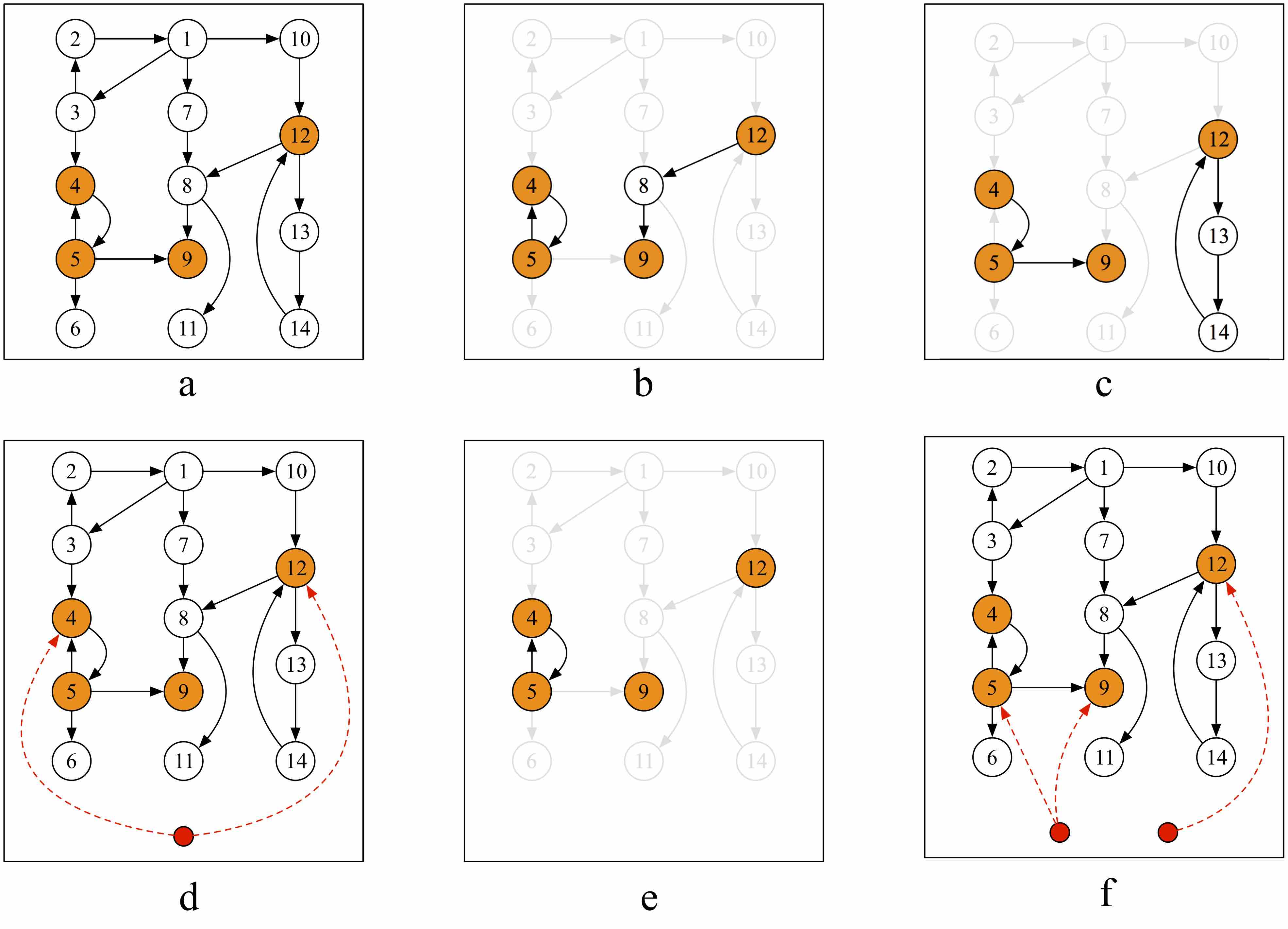
Figure 1: An illustration example of the target control problem. There are 14 nodes in the network (a). The subset nodes are colored with orange, where the target node set is selected as $S=\{v_{4},v_{5},v_{9},v_{12}\}$. In (b), a path $v_{12}v_{8}v_{9}$ and a circle $v_{4}v_{5}v_{4}$ cover the subset nodes. In (c), a path $v_{4}v_{5}v_{9}$ and a circle $v_{12}v_{13}v_{14}v_{12}$ cover the subset nodes. (d) According to (b) or (c) only one external source colored with red is necessary to control the target subset. (e) However, if we select the control source through employing maximum matching (MM) algorithm, the control paths and circles are depicted in (e). (f) According to (e), the number of external control sources is 2. This evidently shows that selecting the control sources based on MM algorithm may not achieve the optimal solution.

Lemma 3

[18] The vertex set $S$ corresponding to $\mathbf{X}_{1}$ in equation (4) is structurally controllable if $S$ can be covered by a union of cacti structure contained in the digraph $G(A,B)$.

From Lemmas 1-3, it is known that when $S=V$ the target controllability problem is reduced to the traditional structural controllability problem, which can be well solved either by employing the maximum matching (MM) algorithm. When $S\subset V$, the MM algorithm becomes inapplicable and currently there is no algorithm to address this issue as the target controllability problem becomes fundamentally different. An example in Figure 1 is presented to illustrate that MM algorithm does not work for the target control problem. Therefore, determining the minimum number of external control sources for ensuring the target controllability is to be investigated in the following Sections.

II-B Converting the target controllability problem into the path cover problem in Graph Theory

For a graph network $D=(V,E)$, define a set of simple directed paths $P=\{v_{a_{k,1}}v_{a_{k,2}}...v_{a_{k,p_{k}}}|k=1,2,...,|P|\}$ where $p_{k}$ is the length of the $k$th directed path, $a_{k,i}$ is the index of the $i$th vertex in $V$ along the $k$th directed path and $|P|$ is the total number of paths. Also, define a set of simple directed circles $\mathcal{C}=\{v_{b_{k,1}}v_{b_{k,2}}...v_{b_{k,c_{k}}}v_{b_{k,1}}|k=1,2,...,|\mathcal{C}|\}$ where $c_{k}$ is the length of the $k$th circle, $b_{k,i}$ is the index of the vertex on the $k$th circle and $|\mathcal{C}|$ is the total number of circles. For the path set $Q=\{v_{l_{k,1}}v_{l_{k,2}}...v_{l_{k,q_{k}}}|k=1,2,...,|Q|\}$ where $q_{k}$ is the length of the $k$th path, $l_{k,i}$ is the index of the vertex in $V$ along the $k$th path and $|Q|$ is the total number of paths, define the nodes covered by $Q$ as $Cover(Q)=\{v_{l_{k,i}}|i=1,2,...,q_{k},k=1,2,...,|Q|\}$.

By Lemmas 1-3, for a given target node set $S$, the target controllability problem can be converted into the following path cover problem:

$$\begin{array}[]{lll}argmin_{P}&|P|^{+}\\ s.t.&|Cover(P\cup\mathcal{C})|=\sum_{k=1}^{|P|}p_{k}+\sum_{k=1}^{|\mathcal{C}|}c_{k}\\ &S\subseteq Cover(P\cup\mathcal{C})\end{array}$$ (5)

where $|P|^{+}=max\{|P|,1\}$ which is to consist with the case when all the nodes in $S$ exist and only exist in a circle path. Therefore what we want to do is to find one feasible solution that $|P|$ is minimal such that every node exists and only exists in $P\cup\mathcal{C}$ for at most once. Therefore, to guarantee that all the nodes in $S$ are target controllable, at least $|P|$ control sources should be allocated and the first node of each directed path should be connected to a different control source. Thus, minimizing the number of control sources is equivalent to minimizing $|P|$ in the above path cover problem.

III Model Transformation to Network Flow Problems

In the last section, we have shown that the original target controllability problem is equivalent to a path cover problem, in which the minimum number of external control sources equals the minimum number of paths. In this section, by firstly presenting some preliminary knowledge and definitions in Section III-A, we shall then propose a graph transformation method in Section III-B to solve the path cover problem. An example is shown in Figure 2. In Section III-C, we show that the path cover problem can be further transformed into the maximum network flow problem. In this way, the target controllability problem can be solved exactly as a maximum network flow problem. To verify the validity of the graph transfer, we prove the equality of the transformation in Theorem 3. Finally in Theorem 4, it is shown that the maximum network flow problem can be solved within polynomial time complexity.

III-A Preliminary knowledge and definitions

Some definitions of a network’s maximum flow problem are given as follows [19, 20, 21, 22].

Capacity function: Given a directed graph $D=(V,E)$, capacity function $c(e)$ is a non-negative function defined in $E$. For an arc $e=(v_{i},v_{j})$, $c(e)=c_{ij}$ is called the capacity of an arc $e$.

Capacity network: Given a directed graph $D=(V,E)$ and its capacity function $c(e)$, $D=(V,E,c(e))$ is called the capacity network.

Flow of the capacity network: Given a capacity network, flow $f(e)$ is a function defined in $E$. For an arc $e=(v_{i},v_{j})$, $f(e)=f_{ij}$ is called the flow value on arc $e$, which is bounded by $c(e)$. If $f(e)$ is an integer, we call it an integer flow.

Source, sink and intermediate vertices: In a capacity network, the source node is denoted as $v_{s}$ whose in-degree equals zero. The sink node is denoted as $v_{t}$ whose out-degree equals zero. All the other nodes are called intermediate vertices.

Capacity constraints : For every arc $e$ in $E$, its flow $f(e)$ cannot exceed its capacity $c(e)$, i.e., $\forall e=(v_{i},v_{j})\in E$,

$$0\leq f_{ij}\leq c_{ij}.$$ (6)

Conservation constraints: For every intermediate vertex, the sum of the flows entering it (in-flow) must equal the sum of the flows exiting it (out-flow). Namely $\forall v_{i}\in V-\{v_{s},v_{t}\}$,

$$\sum_{(v_{i},v_{j})\in E}f_{ij}-\sum_{(v_{j},v_{i})\in E}f_{ji}=0.$$ (7)

Feasible flow: For a capacity network with source and sink, a flow $f=\{f_{ij}\}$ from $v_{s}$ to $v_{t}$ is called a feasible flow if flow $f$ satisfies the capacity constraints and conservation constraints simultaneously. There may be multiple source and sink nodes in a network. The value of a feasible flow $f$ is defined as

$$v(f)=\sum_{(v_{s},v_{j})\in E}f_{sj}=\sum_{(v_{j},v_{t})\in E}f_{jt}.$$ (8)

If all $f_{ij}$ are integers, $f$ is called integral feasible flow.

Lower bounds and upper bounds: Given a directed graph $D=(V,E)$, for an edge $e\in E$, the lower bound flow $l(e)$ and upper bound flow $c(e)$ are two non-negative functions defined in $A$ respectively with $l(e)\leq c(e)$.

Feasible circulation: A circulation $f$ is a flow of $D(V,E)$ such that

$$\forall v_{i}\in V,\sum_{(v_{i},v_{j})\in E}f_{ij}-\sum_{(v_{j},v_{i})\in E}f_{ji}=0.$$ (9)

A feasible circulation is a circulation $f$ of $D(V,E)$ such that

$$\forall e=(v_{i},v_{j})\in E,l(e)\leq f(e)\leq c(e).$$ (10)

III-B From the path cover problem to the network flow problem

According to the path cover problem described in Section II-B, we are now endeavoring to find a path set $P$ with the minimal cardinality $|P|$ such that the given target node set $S\subseteq Cover(P\cup\mathcal{C})$. To introduce the concept flow into the path cover problem, we artificially add a source $v_{s}$ and a sink $v_{t}$ into $D(V,E)$. And for every intermediate vertex $v_{i}$ in $D(V,E,v_{s},v_{t})$, there is an arc entering $v_{i}$ from $v_{s}$ with $c((v_{s},v_{i}))=1$ and an arc exiting $v_{i}$ to $v_{t}$ with $c((v_{i},v_{t}))=1$. For $v_{s}$ and $v_{t}$, there is an arc from $v_{t}$ to $v_{s}$ with capacity $c((v_{t},v_{s}))=\infty$. For each arc $e\in E$, we set its capacity as $c(e)=1$. Now we convert a directed network $D(V,E)$ to a capacity network $D(V,E,v_{s},v_{t},c(e))$. This is illustrated in Figures 2 (a)-(b).

Considering the problem we aim to solve, for every vertex $v_{sub}$ in $S$, there should be one and only one path in the path set $P$ covering $v_{sub}$. In the following, we will introduce a graph transfer method to ensure fulfilling this condition.

Graph transfer - node splitting: We split a node $v\in V$ into two types of virtual vertices $v^{in}$ and $v^{out}$, respectively. Therefore, as shown in Figure 2 (c), the network contains three types of nodes. The first type of nodes are the source and sink node $v_{s}$ and $v_{t}$. The second type of nodes are $v^{in}_{sub}$ ($v_{sub}\in S$) and $v^{in}_{i}$ ($v_{i}\in V-S$) , the original arcs (edges) entering the node $v_{sub}$ or $v_{i}$ now enter $v_{sub}^{in}$ or $v_{i}^{in}$. Similarly, the third type of nodes correspond to $v_{sub}^{out}$ and $v_{i}^{out}$, by which the arcs exiting node $v_{sub}$ or $v_{i}$ now exit $v_{sub}^{out}$ or $v_{i}^{out}$. Besides, for every pair $v_{sub}^{in}$ and $v_{sub}^{out}$, we add an arc $e=(v_{sub}^{in},v_{sub}^{out})$ from $v_{sub}^{in}$ to $v_{sub}^{out}$ with lower bound $l(e)=1$ and upper bound $c(e)=1$. For other nodes $v_{i}\in V-S$, the process of splitting is same as that for $v_{sub}$ except that the lower bound is zero, viz. $l(e)=0$.

Node splitting converts a capacity network into a capacity network with lower bounds and upper bounds $D^{\prime}=(V^{\prime},E^{\prime},v_{s},v_{t},l(e^{\prime}),c(e^{\prime}))$ where $V^{\prime}=\{v^{in},v^{out}\}$ and $E^{\prime}=E\cup\{(v^{in},v^{out})\}$. In the following paragraphs, we will show how to convert a path cover problem to a maximum flow problem.

Theorem 1

The feasible circulation of the network $D^{\prime}=(V^{\prime},E^{\prime},v_{s},v_{t},l(e^{\prime}),c(e^{\prime}))$ corresponds to a structurally controllable subset $S\subseteq V$ of the linear system $(A,B,C)$.

Proof. The feasible circulation of the capacity network $D$ satisfies the capacity constraints and the conservation constraints. Specifically, for the nodes in the subset $S$, we have

$$f\left((v^{in}_{sub},v^{out}_{sub})\right)=1.$$

Thus, the flows of the arcs from $v_{s}$ to the nodes in the subset $S$ are exactly 1. The flows from $v_{s}$ to $v_{t}$ are control paths, while the flow from $v_{i}$ to itself is a circle. Then every node in $S$ is on a certain control path or circle as $f\left((v^{in}_{sub},v^{out}_{sub})\right)=1$. According to Lemma 1, the subset of the linear system $G$ is structurally controllable. $\Box$

To show the existence of the feasible circulation, we introduce another graph transfer method for constructing the associate graph, which is shown in Figure 2 (e).

Constructing the associate graph: Given a capacity network with lower bounds and upper bounds

$$D^{\prime}=\left(V^{\prime},E^{\prime},v_{s},v_{t},l(e^{\prime}),c(e^{\prime})\right),$$

an additional source $v_{s}^{add}$ and an additional sink $v_{t}^{add}$ are added into the network. For every node $v_{i}\in V^{\prime}$, a new arc $e$ is added from $v_{s}^{add}$ to $v_{i}$ with $l(e)=0$ and $c(e)=\sum_{e^{\prime}=(v_{j},v_{i})\in E^{\prime}}l(e^{\prime})$. And a new arc $e$ is added from $v_{i}$ to $v_{t}^{add}$ with $l(e)=0$ and $c(e)=\sum_{e^{\prime}=(v_{i},v_{j})\in E^{\prime}}l(e^{\prime})$. Meanwhile the original arcs in the network $D^{\prime}$ decrease their $l(e^{\prime})$ to zero and $c(e^{\prime})$ to $c(e^{\prime})-l(e^{\prime})$. The new network, termed associate graph hereafter, is $D^{\prime\prime}=(V^{\prime\prime},E^{\prime\prime},c^{\prime}(e^{\prime\prime}))$ with all $l^{\prime}(e^{\prime\prime})\equiv 0$, where

$$\begin{split}V^{\prime\prime}=V^{\prime}\cup\{v_{s}^{add},v_{t}^{add}\},\end{split}$$ (11)

$$\begin{split}E^{\prime\prime}=E^{\prime}\cup\{(v_{s}^{add},v_{i})|v_{i}\in V^{\prime}\}\cup\{(v_{i},v_{t}^{add})|v_{i}\in V^{\prime}\},\end{split}$$ (12)

$$\begin{split}\forall v_{i}\in V^{\prime},~{}c^{\prime}(v_{s}^{add},v_{i})&=\sum_{e^{\prime}=(v_{j},v_{i})\in E^{\prime}}l(e^{\prime}),\\ c^{\prime}(v_{i},v_{t}^{add})&=\sum_{e^{\prime}=(v_{i},v_{j})\in E^{\prime}}l(e^{\prime}),\end{split}$$ (13)

$$\begin{split}\forall e^{\prime}=(v_{i},v_{j})\in E^{\prime},~{}c^{\prime}(e^{\prime})=c(e^{\prime})-l(e^{\prime}).\end{split}$$ (14)

Lemma 4

[19] Iff the value of the maximum flow of the associate graph $D^{\prime\prime}$ from $v_{s}^{add}$ to $v_{t}^{add}$ is equal to the sum of lower bound values of all arcs in the capacity network $D^{\prime}$, the feasible circulation of $D^{\prime}$ exists.

Theorem 2

The feasible circulation of the network $D^{\prime}$ converted from the linear system $G(A,B,C)$ always exists.

Proof. As the source $v_{s}$ and the sink $v_{t}$ are connected to every node in $V$, $v_{s}$ is connected to every $v^{in}$ and $v_{t}$ is connected to every $v^{out}$. Thus, there is always a circulation from $v_{s}^{add}$ to $v_{t}^{add}$, viz. $v_{s}^{add}v_{sub}^{out}...v_{t}v_{s}...v_{sub}^{in}v_{t}^{add}$. Obviously, in the associate graph $D^{\prime\prime}$, the value of the maximum flow from $v_{s}^{add}$ to $v_{t}^{add}$ equals the number of the nodes in the subset $S$. In the capacity network $D^{\prime}$, only the arcs from $v_{sub}^{in}$ to $v_{sub}^{out}$ have the lower bound value $l(e)=1$ while the lower bounds of other acrs are zero. Thus, the sum of lower bound values of all arcs in $D^{\prime}$ is also equal to the number of nodes in the subset $S$. According to Lemma 4, the feasible circulation of $D^{\prime}$ always exists. $\Box$

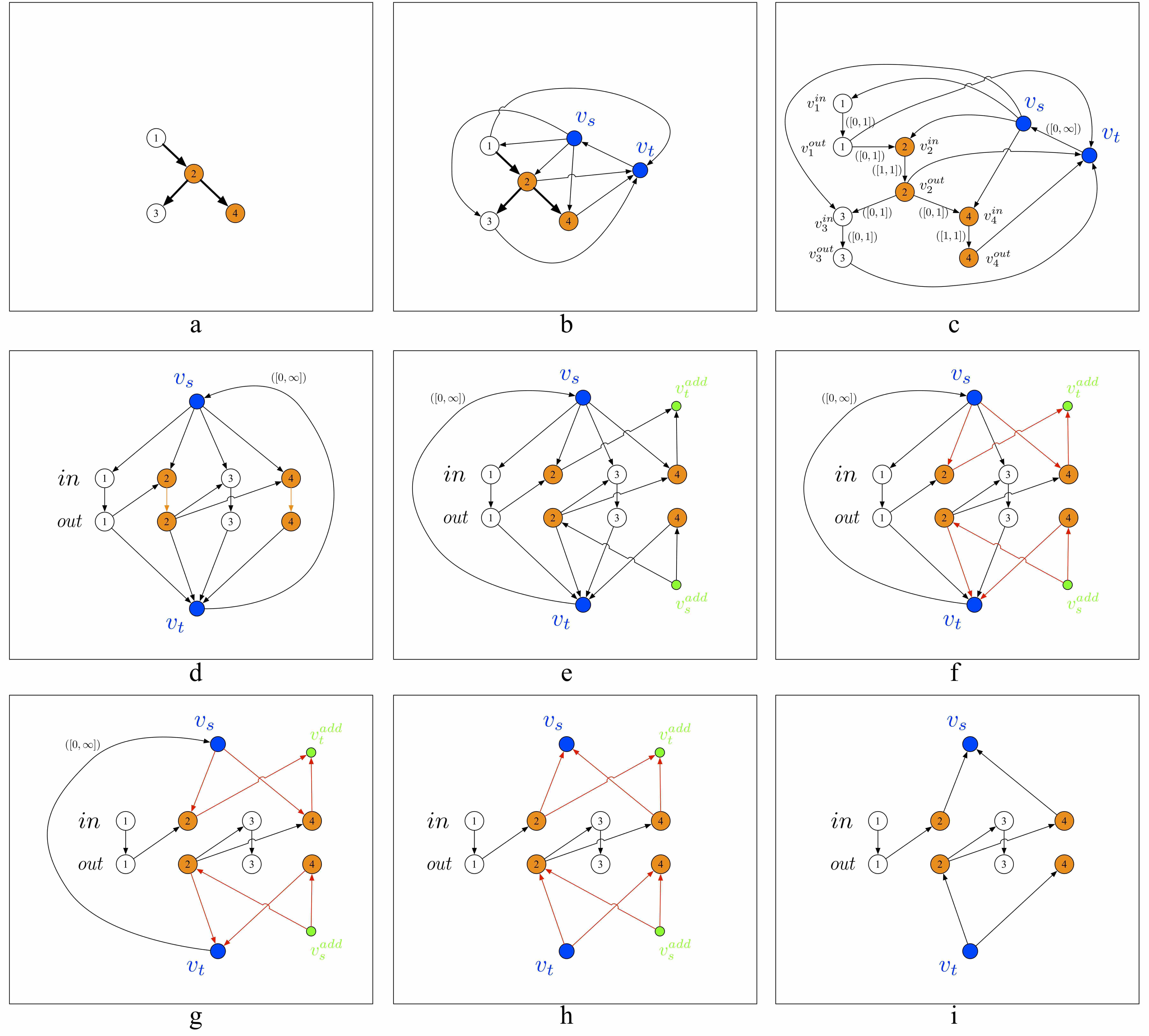
Figure 2: The procedure of graph re-construction to transform the problem to a network flow problem. (a) The network we aim to control. It contains 4 nodes and 3 edges with node 2 and node 4 being in the target set. (b) By adding a source $v_{s}$, a sink $v_{t}$, arcs from $v_{s}$ to other intermediate vertices and arcs from other intermediate vertices to $v_{t}$, the network can be converted into a capacity network. (c) After applying the method of splitting the nodes, the network arc capacities contain lower bounds and upper bounds, which are respectively represented by the left and right numbers in the brackets beside the arcs. (d) By rearranging the position of nodes, the equivalent graph is formed with a source $v_{s}$, a sink $v_{t}$, a set of in-nodes and a set of out-nodes. The orange lines from $v_{2}^{in}$ to $v_{2}^{out}$ and from $v_{4}^{in}$ to $v_{4}^{out}$ are the arcs with lower bounds $l(a)=1$ and upper bound $c(a)=1$. (e) After applying the graph transfer method of constructing the associate graph, the orange lines are replaced by the arcs from $v_{s}^{add}$ and to $v_{t}^{add}$, which transforms the network with lower bounds and upper bounds of the capacity network. (f) The flow of the red lines is 1 and the flow of the black lines is 0. The flows in the graph form a feasible circulation. (g) To find the minimum flow from $v_{s}$ to $v_{t}$, the arcs from $v_{s}$ to $v_{1}^{in}$ and $v_{3}^{out}$ and the arcs from $v_{1}^{out}$ and $v_{3}^{out}$ to $v_{t}$ can be removed as their flow is always 0. (h) The solution to the minimum flow problem is equivalent to solving the maximum flow problem from $v_{t}$ to $v_{s}$. In the network, the direction of the arcs from $v_{s}$ to $v_{2}^{in}$ and $v_{4}^{in}$ and the arcs from $v_{2}^{out}$ and $v_{4}^{out}$ to $v_{t}$ should be reversed. (i) While finding the maximum flow from $v_{t}$ to $v_{s}$, the flow of the arcs from $v_{s}^{add}$ to $v_{2}^{out}$ and $v_{4}^{out}$ and the arcs from $v_{2}^{in}$ and $v_{4}^{out}$ to $v_{t}^{add}$ should be always zero. Thus these arcs can be removed. Finally, the structural control problem of (a) is equivalent to the maximum flow problem from $v_{t}$ to $v_{s}$ in (i).

Based on the above Lemmas and Theorems, for a given target set in $D(V,E)$ that corresponds to a linear system $G(A,B,C)$ in (1) as illustrated in Figure 2 (a), we can re-construct a new graph network $D^{(N)}=(V^{(N)},E^{(N)})$, and convert it to a capacity network $D^{(N)}=(V^{(N)},E^{(N)},v_{s},v_{t},c(e))$. The procedures are described as follows.

1. For every node $v\in V$, split it into two nodes $v^{in}$ and $v^{out}$. Define a node set $V^{(I)}=\{v^{{in}}|v\in V\}$, $V^{(O)}=\{v^{{out}}|v\in V\}$.

2. Define $V^{(N)}=V^{(I)}\cup V^{(O)}\cup\{v_{s},v_{t}\}$ where $v_{s}$ represents the source and $v_{t}$ represents the sink. By setting the upper bound of each edge as $c\left((v_{i},v_{j})\right)=1$ where $v_{i},v_{j}\in V^{(N)}$ and lower bound as $l((v_{sub}^{in},v_{sub}^{out}))=1$ and $l((v_{i},v_{j}))=0$ where $(v_{i},v_{j})\notin E-\{(v_{sub}^{in},v_{sub}^{out})\}$, we build a flow network denoted as $(D^{(N)},cap)$ where $cap$ denotes the capacity function.

3. Construct the edge sets $E^{(1)}=\{(v_{t},v^{out})|v\in S\}$ , $E^{(2)}=\{(v^{(in)},s)|v\in S\}$, $E^{(3)}=\{(v^{in},v^{out})|v\not\in S\}$, $E^{(4)}=\{(v^{out}_{i},v^{in}_{j})|(v_{i},v_{j})\in E\}$ and $E^{(N)}=E^{(1)}\cup E^{(2)}\cup E^{(3)}\cup E^{(4)}$.

4. For each edge $(v_{i},v_{j})\in E^{(N)}$, set its upper capacity as $c((v_{i},v_{j}))=1$.

Finally, by defining a residual network as $(D^{(N)},cap,flow)$ where $flow(e)$ is the flow of edge $e$ such that $l(e)\leq flow(e)\leq c(e)$, we can convert the path cover problem into a maximum network flow problem in $(D^{(N)},cap,v_{s},v_{t})$ as shown in Figure 2 (i) from $v_{s}$ to $v_{t}$.

An example for the graph re-construction is illustrated in Fig.2 (a)-Fig.2 (i). For a given linear system $(A,B,C)$, the adjacent matrix $A$ gives the topology information of the capacity network. An arc $e=(v_{i},v_{j})$ is in the arc set $E$ if $A(i,j)=1$. The source $v_{s}$ and the sink $v_{t}$ can be treated as the same node as they both represent the set of external drivers defined by the control matrix $B$, viz. there is an arc from $v_{t}$ to $v_{s}$ with capacity of infinity $c\left((v_{t},v_{s})\right)=\infty$. As they are external drivers, there are arcs from $v_{s}$ to every vertex in the network and arcs from every vertex to $v_{t}$. As capacity function $c(e)=1,\forall e\in E$, the sum of out-flow of $v_{s}$ or the sum of in-flow of $v_{t}$ is equal to the number of external drivers.

The detailed process of re-constructing the edge sets in the procedure $c)$ is shown in Figs. 2 (c)-(i). After the procedure $b)$, we rearrange the position of the nodes as shown in Figs.2 (c)-(d). For this capacity network with upper bounds and lower bounds, we have to re-construct it by means of constructing the associate graph as described before. An additional source $v_{s}^{add}$ and an additional sink $v_{t}^{add}$ are added into the network to transform the capacity network with upper and lower bounds to the associate network with its all lower bounds $l(e)=0$ as illustrated in Figure 2 (e). Based on the Theorem 1, to find the structurally controllable scheme with the minimal external sources, we start from the feasible circulation, which is shown in Figure 2 (f). While ensuring the feasibility of the circulation in $D^{\prime}$, the control scheme with the minimal controllers can be achieved as long as the value of flow from $v_{s}$ to $v_{t}$ decreases to the minimum. Thus for the vertex $v_{i}\in V^{\prime}-S$, the flow of the arcs from $v_{s}$ to $v_{i}^{in}$ or from $v_{i}^{out}$ to $v_{t}$ is zero. And the arcs can be removed, which is shown in Figure 2 (g). The minimum flow problem from $v_{s}$ to $v_{t}$ can be converted to the maximum flow problem from $v_{t}$ to $v_{s}$, which is shown in Figure 2 (h). In order to find the maximum flow from $v_{t}$ to $v_{s}$, the arcs from $v_{s}^{add}$ or to $v_{t}^{add}$ can be removed as they cannot contribute to the increase of the flow, which is shown in Figure 2 (i).

III-C Maximum-flow based target path-cover (MFTP) algorithm

In this subsection, we focus on discussing how to locate the circle path set $\mathcal{C}$ and the simple directed path set $P$ containing the least number of simple paths $|P|$ to cover $S$. In the previous subsection, we carried out graph transformation method to address the path cover problem through solving the maximum network flow problem $(D^{(N)},cap,v_{s},v_{t})$ from $v_{s}$ to $v_{t}$. In the following, an algorithm named “maximum-flow based target path-cover” (MFTP) is first proposed regarding how to obtain the maximum flow of $(D^{(N)},cap,v_{s},v_{t})$ from $v_{t}$ to $v_{s}$ in Figure 2 (i). In the next subsection, it will be shown in Theorems 3-4 that the solution of the original target controllability problem is equivalent to finding the maximum flow in $(D^{(N)},cap,v_{s},v_{t})$ which can be solved by introducing the Dinic algorithm with a polynomial complexity. The MFTP algorithm is presented as follows.

1. For a given graph network $D(V,E)$, build a new graph network $D^{(N)}=(V^{(N)},E^{(N)})$ according to procedure (a)-(d) described in Section III-B.

2. Define $E^{(F)}=\{(v_{i},v_{j})|(v^{out}_{i},v^{in}_{j})\in E^{(4)},flow((v^{out}_{i},v^{in}_{j}))=1\}$. Obtain the edge set $E^{(F)}$ by applying the Dinic algorithm [23] [24] to the maximum flow problem in $(D^{(N)},cap,v_{s},v_{t})$. Let directed path set $P\leftarrow\emptyset$, circle path set $\mathcal{C}\leftarrow\emptyset$, do the following steps:

3. For each node $v_{i}\in S$, if there does not exist a node $v_{j}\in V$ such that $(v_{i},v_{j})\in E^{(F)}$ or $(v_{j},v_{i})\in E^{(F)}$, then update $P\leftarrow P\cup\{(v_{i})\}$, i.e., add all the simple paths that contain only a single node $v_{i}$ to $P$.

4. Find one node $v_{1}$ such that there exist no node $v_{0}$ satisfying $(v_{0},v_{1})\in E^{(F)}$. Continue the process to find nodes $v_{2},...,v_{p}$ which form a unique sequence $v_{1}v_{2}...v_{p}$ such that $(v_{1},v_{2}),(v_{2},v_{3}),...,(v_{p-1},v_{p})\in E^{(F)}$ until there does not exist $v_{p+1}$ satisfying that $(v_{p},v_{p+1})\in E^{(F)}$. Then, add the path $v_{1}v_{2}...v_{p}$ to $P$, i.e., update $P\leftarrow P\cup\{v_{1}v_{2}...v_{p}\}$ and delete all the edges $(v_{1},v_{2}),(v_{2},v_{3}),...,(v_{p-1},v_{p})\in E^{(F)}$.

5. Repeat Step 4 until no more $v_{1}$ can be found.

6. If there exists any edge in $E^{(F)}$, then for an arbitrary edge $(v_{1},v_{2})\in E^{(F)}$, find a unique sequence $v_{3},v_{4},...,v_{c}$ such that $(v_{2},v_{3}),...,(v_{c-1},v_{c}),(v_{c},v_{1})\in E^{(F)}$. As will be proved in Theorem 3 such node $v_{1}$ always exists. Then, add the path $v_{1}v_{2}...v_{c}v_{1}$ to $\mathcal{C}$ and update $\mathcal{C}\leftarrow\mathcal{C}\cup\{v_{1}v_{2}...v_{c}v_{1}\}$, and delete all the edges $(v_{1},v_{2}),(v_{2},v_{3}),...,(v_{c},v_{1})\in E^{(F)}$.

7. Repeat the process in Step 6 until $E^{(F)}$ becomes an empty set, and all the simple paths and circles in $P$ and $\mathcal{C}$ are finally obtained.

III-D Equivalence of the path cover problem and the maximum network flow problem

In this subsection, we will prove that the solution of the original target controllability problem is equivalent to finding the maximum flow in $(D^{(N)},cap,v_{s},v_{t})$ which can be solved by introducing the Dinic algorithm with a polynomial complexity, and the number of the minimum external sources equals the minimum number of simple paths in $P$ given by $min\{|P|\}=|S|-maxflow(D^{(N)},cap,s,t)$.

Theorem 3

The target controllability problem in the original graph network $D(V,E)$ in (5) is equivalent to the converted maximum flow problem $maxflow(D^{(N)},cap,v_{s},v_{t})$.

Proof. We need to prove the following four statements:

1. Any feasible flow in the flow network $(D^{(N)},cap)$ corresponds to a feasible solution of the original target controllability problem in $D(V,E)$. This is to prove that there exists an injective mapping from a feasible residual network $(D^{(N)},cap,flow)$ with integral flow to the set $P\cup\mathcal{C}$ such that $S\subseteq P\cup\mathcal{C}$ and each element of $S$ exists and only exists once in $P\cup\mathcal{C}$. Here, the residual network refers to the network $(D^{(N)},cap)$ with its flow reaching maximum.

As we can build $P$ and $\mathcal{C}$ based on the obtained $E^{(F)}$ from the above described algorithm, we only need to prove that its solution is a feasible solution. Note that here we are not discussing on how to build $P$ and $\mathcal{C}$ when a maximum flow has been achieved. Instead, we are proving that any

$$E^{(F)}=\{(v_{i},v_{j})|(v_{i}^{out},v_{j}^{(in)})\in E^{(4)},flow((v_{i}^{out},v_{j}^{in}))=1\}$$

corresponding to a feasible flow gives a feasible solution of (5) in the residual network $(D^{(N)},cap,flow)$ with only integral flow.

To this end, firstly, we prove that

1. $\forall v_{i}\in V:$ there exists at most one $v_{j}\in V$ such that $(v_{i},v_{j})\in E^{(F)}$, or there exists at most one $v_{j}\in V$ such that $(v_{j},v_{i})\in E^{(F)}$. This is to prove that there exists at most one node $v_{j}\in V$ such that $(v_{i}^{out},v_{j}^{in})\in E^{(F)}$ and $flow((v_{i}^{out},v_{j}^{in}))=1$.

   Consider the input edges of a node $v_{i}^{out}$: if $v_{i}\in S$, then there exists one and only one edge $(v_{t},v_{i}^{out})\in E^{(1)}\subseteq E^{(N)}$; if $v_{i}\not\in S$, then there exists one and only one edge $(v_{i}^{in},v_{i}^{out})\in E^{(3)}\subseteq E^{(N)}$. By combining both cases, there exists only one edge with capacity 1 pointing to $v^{out}_{i}$. As the flow in the network is always an integer, there exists at most one $v_{j}\in V$ such that $(v_{i}^{out},v_{j}^{in})\in E^{(4)}$ and $flow((v_{i}^{out},v_{j}^{in}))=1$. Similarly, considering that $v_{i}^{in}$ has at most one output edge belonging to either $E^{(2)}$ or $E^{(3)}$ depending on whether $v_{i}$ belongs to $S$ or not, then there exists at most one $v_{j}\in V$ such that $(v_{j},v_{i})\in E^{(F)}$.

2. If Step 3 of MFTP algorithm can be processed, a simple path can always be located in which all nodes are covered only once.

   In the case that we cannot find a simple path or Step 3 goes into an infinite loop, then there must exist a circle path and the algorithm goes into an infinite loop. In this case, on the path $v_{1},v_{2},....,v_{p},...$, there must exist repetitious nodes. Without loss of generality, we assume that the first repetitious node pair is $v_{i}$ and $v_{j}$ with ($i<j$), i.e. $v_{i}$ and $v_{j}$ are the same node appearing in different places on the path. If $v_{i}=v_{1}$, then $(v_{j-1},v_{j})=(v_{j-1},v_{i})=(v_{j-1},v_{1})\in E^{(F)}$, which contradicts the fact that $v_{1}$ does not have any input; if $v_{i}\neq v_{1}$, then $(v_{j-1},v_{j})=(v_{j-1},v_{i})=(v_{i-1},v_{i})\in E^{(F)}$. But it is known that $v_{i-1}\neq v_{j-1}$ as $v_{i}$ and $v_{j}$ are the first repetitious node pair, which manifests that $v_{i}$ has two input edges from $v_{i-1}$ and $v_{j-1}$ respectively. This contradicts the fact that the input degree of each node cannot be greater than $1$. Thus we draw the conclusion that a simple path can always be located as long as Step 3 can be processed.

3. If the Step 4 of MFTP algorithm has been accomplished, then a simple circle can always be located by implementing Step 5 .

   At this stage, we cannot find any node that has an output edge but does not have any input edge; otherwise, the proposed algorithm goes back to Step 3. Note that the input degree of all nodes is not smaller than 1 while the input degree cannot be greater than 1. Therefore, the remaining nodes have one and only one input edge. Then, by starting from an arbitrary node, we can always come back to this node and a circle can be uniquely found, and the remaining edges exist in one and only one circle.

4. All the nodes exist and only exist once in $P\cup\mathcal{C}$ and $S\subseteq cover(P\cup\mathcal{C})$.

   This is obvious since if a node has any input or output edge existing in $E^{(F)}$, then it must have been deleted in Step 3 or Step 5; otherwise, it would contradict the fact that all input and output degrees are not greater than $1$. If one node $v\in S$ but it does not have an edge in $E^{(F)}$, then it will be added into $P$ in Step 2.

2. The flow from $v_{t}$ to $v_{s}$ of the residual network $(D^{(N)},cap,flow)$ equals $|S|-|P|$.

Based on the conservation constraints in Section 3.1, when the total flow of the residual network $(D^{(N)},cap,flow)$ equals $f$, we could obtain $f$ paths on the flow network:

$$\begin{array}[]{lll}v_{t}v_{p_{1,1}}v_{p_{1,2}}...v_{p_{1,d_{1}}}v_{s},\\ v_{t}v_{p_{2,1}}v_{p_{2,2}}...v_{p_{2,d_{2}}}v_{s},\\ ~{}~{}~{}~{}~{}~{}~{}~{}~{}~{}~{}~{}~{}~{}~{}~{}~{}\vdots\\ v_{t}v_{p_{f,1}}v_{p_{f,2}}...v_{p_{f,d_{f}}}v_{s}.\end{array}$$ (15)

where all these paths start from $v_{t}$ and end at $v_{s}$, and the flow of an edge $(v_{i},v_{j})\in E^{(N)}$ equals the occurrence number of $(v_{i},v_{j})$ in all paths. Thus, for the $i$-th path, $(v_{t},v_{p_{i,1}})\in E^{(1)},v_{p_{i,1}}\in V^{(O)}$ as $v_{t}$ only points to $V^{(O)}$; and $(v_{p_{i,1}},v_{s})\in E^{(2)},v_{p_{d_{i},1}}\in V^{(I)}$.

Consider that $\forall v^{out}\in V^{(O)}$, its output edges all belong to $E^{(4)}$. Therefore, as long as $v_{p_{i,j}}\in V^{(O)}$, $(v_{p_{i,j}},v_{p_{i,j+1}})\in E^{(4)}$, and $v_{p_{i,j+1}}\in V^{(I)}$. Also, as there is no output edge of $v_{s}$, $v_{p_{i,j}}\neq v_{s}$. For $\forall v^{in}\in V^{(I)}$, the edges starting from $v^{in}$ belong to either $E^{(2)}$ or $E^{(3)}$. As all the edges in $E^{(2)}$ point to $v_{s}$, if $v_{p_{i,j}}\in V^{(I)}$ and $j<d_{i}$, then $(v_{p_{i,j}},v_{p_{i,j+1}})\in E^{(3)}$ and $v_{p_{i,j+1}}\in V^{(O)}$. Therefore, for each path $i$, $d_{i}$ is an even number. And $\forall 1\leq j\leq\frac{d_{i}}{2}$, $v_{p_{i},2j-1}\in V^{(O)}$, $v_{p_{i},2j}\in V^{(I)}$ and $(v_{p_{i},2j-1},v_{p_{i},2j})\in E^{(4)}$; $\forall 1\leq j\leq\frac{d_{i}}{2}-1$, $(v_{p_{i},2j},v_{p_{i},2j+1})\in E^{(3)}$. Thus, the $f$ paths can be rewritten as

$$\begin{array}[]{lll}v_{t}v^{out}_{p^{{}^{\prime}}_{1,1}}v^{in}_{p^{{}^{\prime}}_{1,2}}v^{out}_{p^{{}^{\prime}}_{1,2}}v^{in}_{p^{{}^{\prime}}_{1,3}}...v^{in}_{p^{{}^{\prime}}_{1,\frac{d_{1}}{2}+1}}v_{s},\\ v_{t}v^{out}_{p^{{}^{\prime}}_{2,1}}v^{in}_{p^{{}^{\prime}}_{2,2}}v^{out}_{p^{{}^{\prime}}_{2,2}}v^{in}_{p^{{}^{\prime}}_{2,3}}...v^{in}_{p^{{}^{\prime}}_{1,\frac{d_{2}}{2}+1}}v_{s},\\ ~{}~{}~{}~{}~{}~{}~{}~{}~{}~{}~{}~{}~{}~{}~{}~{}~{}~{}~{}~{}~{}~{}~{}~{}~{}~{}~{}\vdots\\ v_{t}v^{out}_{p^{{}^{\prime}}_{f,1}}v^{in}_{p^{{}^{\prime}}_{f,2}}v^{out}_{p^{{}^{\prime}}_{f,2}}v^{in}_{p^{{}^{\prime}}_{f,3}}...v^{in}_{p^{{}^{\prime}}_{1,\frac{d_{f}}{2}+1}}v_{s}.\end{array}$$ (16)

In addition, we have that

$$\begin{split}&E^{(F)}\\ =&\left\{\begin{array}[]{ccccccccccccc}(v_{p^{{}^{\prime}}_{1,1}},v_{p^{{}^{\prime}}_{1,2}}),&(v_{p^{{}^{\prime}}_{1,2}},v_{p^{{}^{\prime}}_{1,3}}),&...,&(v_{p^{{}^{\prime}}_{1,\frac{d_{1}}{2}}},v_{p^{{}^{\prime}}_{1,\frac{d_{1}}{2}+1}})\\ (v_{p^{{}^{\prime}}_{2,1}},v_{p^{{}^{\prime}}_{2,2}}),&(v_{p^{{}^{\prime}}_{2,2}},v_{p^{{}^{\prime}}_{2,3}}),&...,&(v_{p^{{}^{\prime}}_{2,\frac{d_{2}}{2}}},v_{p^{{}^{\prime}}_{2,\frac{d_{2}}{2}+1}})\\ &&\vdots\\ (v_{p^{{}^{\prime}}_{f,1}},v_{p^{{}^{\prime}}_{f,2}}),&(v_{p^{{}^{\prime}}_{f,2}},v_{p^{{}^{\prime}}_{f,3}}),&...,&(v_{p^{{}^{\prime}}_{f,\frac{d_{f}}{2}}},v_{p^{{}^{\prime}}_{f,\frac{d_{f}}{2}+1}})\end{array}\right\}\end{split}$$

Since $E^{(1)}$ and $E^{(2)}$ are built only based on the nodes in the subset $S$, and $E^{(3)}$ is only based on $V-S$, for each path $i$, we conclude that $v_{p^{{}^{\prime}}_{i,1}},v_{p^{{}^{\prime}}_{i,\frac{d_{i}}{2}+1}}\in S$ and $v_{p^{{}^{\prime}}_{i,2}},v_{p^{{}^{\prime}}_{i,3}},...,v_{p^{{}^{\prime}}_{i,\frac{d_{i}}{2}}}\in V-S$. As we know that the capacity of edges is 1, all $v_{p^{{}^{\prime}}_{i,1}}$ are all different, and all $v_{p^{{}^{\prime}}_{i,\frac{d_{i}}{2}+1}}$ are different.

Based on the inductive method, now we prove the following conclusion: when the edge set $E^{(F)}$ only contains the elements of the first $f$ rows (specifically the first $d_{1}+d_{2}+...+d_{f}$ elements), we have $f=|S|-|P|$.

In the first step, we aim to prove by inductive method that by applying the proposed algorithm every time when we add a row into $E^{(F)}$, e.g. the $i$th row is added, we can always find two paths in $P$, one ends at $v_{p^{{}^{\prime}}_{i,1}}$ denoted as $v_{-l_{i}}v_{-l_{i}+1}...v_{p^{{}^{\prime}}_{i,1}}$ and the other starts from $v_{p^{{}^{\prime}}_{i,\frac{d_{i}}{2}+1}}$ denoted as $v_{p^{{}^{\prime}}_{i,\frac{d_{i}}{2}+1}}...v_{r_{i}-1}v_{r_{i}}$.

Firstly, according to the above conclusion that $v_{p^{{}^{\prime}}_{i,1}},v_{p^{{}^{\prime}}_{i,\frac{d_{i}}{2}+1}}\in S$, when $f=0$, i.e. $E^{(F)}=\emptyset$, $P=\{v|v\in S\}$, we can find two paths in $P$, one ends at $v_{p^{{}^{\prime}}_{1,1}}$ denoted as $v_{-l_{1}}v_{-l_{1}+1}...v_{p^{{}^{\prime}}_{1,1}}$ (actually this path is $v_{p^{{}^{\prime}}_{1,1}}$) and the other starts from $v_{p^{{}^{\prime}}_{1,\frac{d_{1}}{2}+1}}$ denoted as $v_{p^{{}^{\prime}}_{1,\frac{d_{1}}{2}+1}}...v_{r_{1}-1}v_{r_{1}}$ (actually this path is $v_{p^{{}^{\prime}}_{1,\frac{d_{1}}{2}+1}}$).

Secondly, suppose that after the $k$th row was added into $E^{(F)}$, we can find those two paths as mentioned above. In the following, we are going to prove that if the $(k+1)$th row was added to $E^{(F)}$, we can still find those two paths.

When we add the $k$th row

$$\{(v_{p^{{}^{\prime}}_{k,1}},v_{p^{{}^{\prime}}_{k,2}}),(v_{p^{{}^{\prime}}_{k,2}},v_{p^{{}^{\prime}}_{k,3}}),...,(v_{p^{{}^{\prime}}_{k,\frac{d_{k}}{2}}},v_{p^{{}^{\prime}}_{k,\frac{d_{k}}{2}+1}})\}$$

into $E^{(F)}$, we can find the two paths, one ends at $v_{p^{{}^{\prime}}_{k,1}}$ denoted as $v_{-l_{k}}v_{-l_{k}+1}...v_{p^{{}^{\prime}}_{k,1}}$ and the other starts from $v_{p^{{}^{\prime}}_{k,\frac{d_{k}}{2}+1}}$ denoted as $v_{p^{{}^{\prime}}_{k,\frac{d_{k}}{2}+1}}...v_{r_{k}-1}v_{r_{k}}$.

If these two paths are the same, then $v_{-l_{k}}=v_{p^{{}^{\prime}}_{k,\frac{d_{k}}{2}+1}}$ and $v_{p^{{}^{\prime}}_{k,1}}=v_{r_{k}}$. The proposed algorithm will delete this path from $P$ and add a circle

$$v_{p^{{}^{\prime}}_{k,1}}v_{p^{{}^{\prime}}_{k,2}}...v_{p^{{}^{\prime}}_{k,\frac{d_{k}}{2}}}v_{p^{{}^{\prime}}_{k,\frac{d_{k}}{2}+1}}v_{-l_{k}+1}...v_{r_{k}-1}v_{p^{{}^{\prime}}_{k,1}}$$

to $\mathcal{C}$. If these two paths are not the same, the proposed algorithm will delete these two paths from $P$ and add an updated path

$$v_{-l_{k}}v_{-l_{k}+1}...v_{p^{{}^{\prime}}_{k,1}}v_{p^{{}^{\prime}}_{k,2}}...v_{p^{{}^{\prime}}_{k,\frac{d_{k}}{2}}}v_{p^{{}^{\prime}}_{k,\frac{d_{k}}{2}+1}}...v_{r_{k}-1}v_{r_{k}}$$

to $P$. Note that we only updated the two or one path we found while all the other paths in $P$ remain unchanged. If the two paths are the same, $v_{p^{{}^{\prime}}_{k,\frac{d_{k}}{2}+1}}$ will be deleted from the set of starting vertices of all paths in $P$. If the two paths are not the same, the new path still starts from $v_{-l_{k}}$, $v_{p^{{}^{\prime}}_{k,\frac{d_{k}}{2}+1}}$ is also deleted from the set of starting vertices of all paths in $P$. This is also valid for the path ending at $v_{p^{{}^{\prime}}_{k,1}}$.

In general, we only delete $v_{p^{{}^{\prime}}_{k,\frac{d_{k}}{2}+1}}$ from the set of starting vertices of all paths in $P$ and $v_{p^{{}^{\prime}}_{k,1}}$ from the set of ending vertices of all paths in $P$. According to the conclusion that $v_{p^{{}^{\prime}}_{i,1}},v_{p^{{}^{\prime}}_{i,\frac{d_{i}}{2}+1}}\in S$, all $v_{p^{{}^{\prime}}_{i,1}}$ are all different in all paths, and all $v_{p^{{}^{\prime}}_{i,\frac{d_{i}}{2}+1}}$ are different, $v_{p^{{}^{\prime}}_{k+1,\frac{d_{k+1}}{2}+1}}\in S$ is still in the set of starting vertices of all paths in $P$ and $v_{p^{{}^{\prime}}_{k+1,1}}\in S$ is still in the set of ending vertices of all paths in $P$, which implies that after the $(k+1)$th row is added to $E^{(F)}$, the two paths can also be found.

Now we have proven that those two paths can always be found each time we add a row into $E^{(F)}$.

In the second step, we aim to prove that $f=|S|-|P|$ is valid when we add the first $f$ rows into $E^{(F)}$.

Firstly, when $f=0$, i.e. $E^{(F)}=\emptyset$, we have $|P|=|S|$ as $P=\{v|v\in S\}$.

Secondly, suppose that $k-1=|S|-|P|$ when $E^{(F)}$ contains $k-1$ rows. In the following, we are going to prove that, if one row

$$\{(v_{p^{{}^{\prime}}_{k,1}},v_{p^{{}^{\prime}}_{k,2}}),(v_{p^{{}^{\prime}}_{k,2}},v_{p^{{}^{\prime}}_{k,3}}),...,(v_{p^{{}^{\prime}}_{k,\frac{d_{k}}{2}}},v_{p^{{}^{\prime}}_{k,\frac{d_{k}}{2}+1}})\}$$

is added to $E^{(F)}$, we have $k=|S|-|P|$, which implies that $|P|$ is reduced by 1 in this case.

To avoid confusion, let $j=\frac{d_{k}}{2}$. According to the proof in the first step, we can always find two paths in the existing $P$, one ends at $v_{p^{{}^{\prime}}_{k,1}}$ denoted as $v_{-l}v_{-l+1}...v_{p^{{}^{\prime}}_{k,1}}$ and the other starts from $v_{p^{{}^{\prime}}_{k,j+1}}$ denoted as $v_{p^{{}^{\prime}}_{k,j+1}}...v_{r-1}v_{r}$. And according to the first step, if these two paths are the same path, the proposed algorithm will delete this path from $P$ and add a circle $v_{p^{{}^{\prime}}_{k,1}}v_{p^{{}^{\prime}}_{k,2}}...v_{p^{{}^{\prime}}_{k,j}}v_{p^{{}^{\prime}}_{k,j+1}}v_{-l+1}...v_{r-1}v_{p^{{}^{\prime}}_{k,1}}$ to $\mathcal{C}$ . Then $|P|$ will be reduced by $1$. If these two paths are not the same, our proposed algorithm will delete these two paths from $P$ and add an updated path

$$v_{-l}v_{-l+1}...v_{p^{{}^{\prime}}_{k,1}}v_{p^{{}^{\prime}}_{k,2}}...v_{p^{{}^{\prime}}_{k,j+1}}...v_{r-1}v_{r}$$

to $P$. Then $|P|$ will be also reduced by $1$. Thus, $f=k=|S|-|P|$ is still valid.

Finally, we obtain that $f=|S|-|P|$.

3. Any feasible solution of the original problem corresponds to an integer feasible flow in the flow network $(D^{(N)},cap)$, and $|S|-|P|$ is no larger than the flow. This is to prove that there exists an injective mapping which maps a path cover $P\cup\mathcal{C}$ in which all nodes in subset $S$ exist and only exist once in a residual network $(D^{(N)},cap,flow)$ with integer flow, and the network flow is not smaller than $|S|-|P|$.

Firstly, for each simple path in $P$, delete the first and last few nodes that do not belong to $S$ such that the first and the end nodes belong to $S$. In the case that all the nodes on the path do not belong to $S$, we delete the whole path. It is seen that such operations do not change the fact that all the nodes in $S$ appear and only appear once in the cover $P\cup\mathcal{C}$.

Secondly, we construct the feasible flow based on transposing the steps as discussed before: we open all the paths and circles at the nodes belonging to $S$ such that the first and last nodes of all new paths belong to $S$. Then, a feasible flow can be constructed from $v_{s}$ to $v_{t}$ for each simple path. Finally, feasible circulations can be constructed based on those nodes that are not in $S$.

4. The maximum flow is the optimal solution of original problem.

From the network flow theory, if the flow capacities of all the links are integers, then for a given integer flow from $v_{s}$ to $v_{t}$, there exists an integer feasible flow , and it can be proven that the maximum flow is also an integer.

At the same time, the maximum flow algorithm guarantees that the maximum flow has been obtained from $v_{t}$ to $v_{s}$.

Based on the proofs of sub problems 1 and 2 above, we could obtain all the paths and circles that cover the subset with the network flow being $|S|-|P|$. On the other hand, there does not exist a solution with a smaller $|P|$; otherwise, we should have obtained a solution which corresponds to feasible flow being $|S|-|P|$. This contradicts with the maximum flow theory.

Based on the four proofs above, we prove the existence and optimality of the proposed method. $\Box$

Theorem 4

Finding the optimal solution of the Maximum Flow Problem in MFTP by Dinic algorithm has a time complexity of $O\left(|V|^{1/2}|E|\right)$.

Proof. The proof can be seen in [25]. The time complexity of original Dinic’s is $O\left(|V|^{2}|E|\right)$ which is fast enough for most graphs. Furthermore, the Dinic’s itself can be optimized to $O\left(|V||E|\log|V|\right)$ with a data structure called dynamic trees.

When the edge capacities are all equal to one, the algorithm has a complexity of $O(|V|^{2/3}|E|)$, and if the vertex capacities are all equal to one, the algorithm has a complexity of $O(|V|^{1/2}|E|)$. Since the graph is transformed from the network with unit capacities for all vertices other than the source and the sink, all edge capacities are equal to $1$ and every vertex $v$ other than $s$ or $t$ either has a single edge emanating from it or has a single edge entering it. According to [25], this kind of network is of type 2 and the time complexity of Dinic’s can be reduced into $O\left(|V|^{1/2}|E|\right)$, i.e. we can solve the Problem 2 which is more general in this complexity. $\Box$

In [4], it is known that we can solve the structural controllability of the entire network by employing MM algorithm with complexity $O(|V|^{1/2}|E|)$. As stated above, our MFTP algorithm has the same time complexity but can deal with more general cases. Actually, a maximum matching problem itself can be solved by transforming it into a network flow problem. Therefore, MFTP is consistent with the MM algorithm when $S=V$ and can be applied to more complicated cases where $S\subset V$ or there are multiple layers in the network.

IV Experimental Results

IV-A Illustration of target control in a simple network

Consider a simple example in Figure 3, the target node set is selected as $S=\{node~{}2,node~{}3,node~{}7,node~{}9\}$. The matrices $A$ and $C$ are given by

$$\begin{split}A=\left(\begin{array}[]{cccccccccccccccccc}0&0&0&0&0&0&0&0&0\\ 1&0&0&0&0&1&0&0&0\\ 0&1&0&0&0&1&0&0&0\\ 0&0&1&0&0&0&1&0&0\\ 0&0&0&0&0&0&0&0&0\\ 0&0&0&0&1&0&0&0&1\\ 0&0&0&0&0&1&0&0&1\\ 0&0&0&0&0&0&0&0&0\\ 0&0&0&0&0&1&0&1&0\\ \end{array}\right),\\ C=\left(\begin{array}[]{cccccccccccccccccc}0&1&0&0&0&0&0&0&0\\ 0&0&1&0&0&0&0&0&0\\ 0&0&0&0&0&0&1&0&0\\ 0&0&0&0&0&0&0&0&1\\ \end{array}\right).\end{split}$$

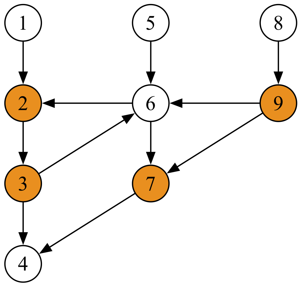
Figure 3: A simple example of the target control problem. There are $9$ nodes in the network with the target set $S$ being $\{node~{}2,node~{}3,node~{}7,node~{}9\}$ colored with orange.

Recall that the objective is to allocate the minimum number of external control sources such that $S$ is controllable. As shown in Section 4, this problem can be converted into the maximum flow problem on the reconstructed flow network in Figure 4 similar to Figure 2 .

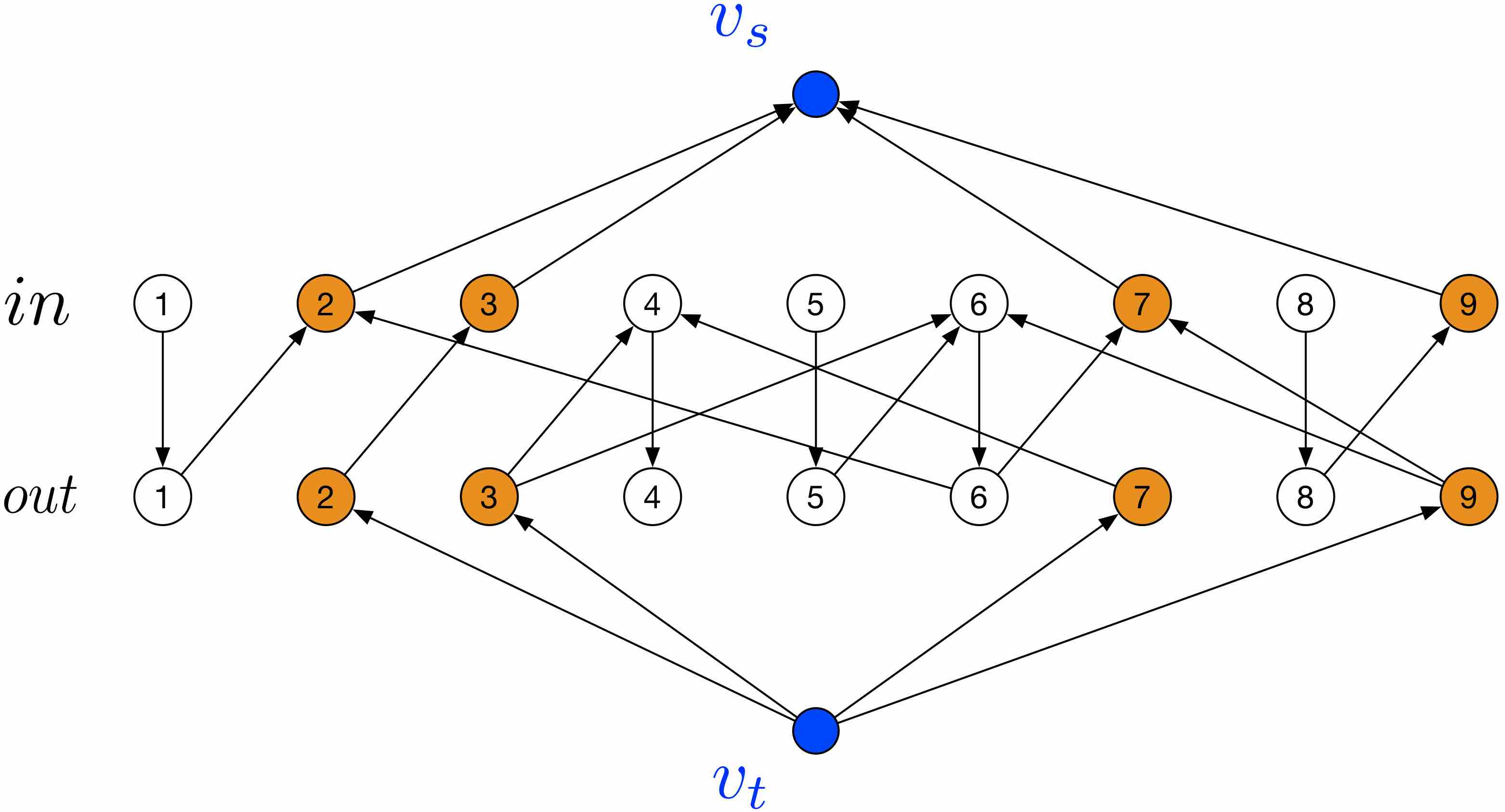
Figure 4: The reconstructed flow network.

Here is a step by step explanation of how this graph is constructed:

1. For the network in Figure 3, we first use the graph transfer methods node splitting to get a graph with node set $V^{(N)}=V\cup V^{(I)}\cup V^{(O)}\cup{v_{s},v_{t}}$ and edge set $E^{(N)}=E\cup\{(v_{s},v_{i}^{in})\}\cup\{(v_{i}^{out},v_{t})\}$.

2. Then use the graph transfer methods associate graph construct and reverse the direction of edges in $\{(v_{s},v_{i}^{in})\}\cup\{(v_{i}^{out},v_{t})\}$ to get the graph shown in Figure 4.

3. After this, use Dinic algorithm to get the maximum flow from $v_{t}$ to $v_{s}$ which is obviously

   $$f(e)=\begin{cases}1,e\in\left\{\begin{array}[]{c}(v_{t},v_{2}^{out}),(v_{2}^{out},v_{3}^{in}),(v_{3}^{in},v_{s}),\\ (v_{s},v_{9}^{out}),(v_{9}^{out},v_{7}^{in}),(v_{7}^{in},v_{s})\\ (v_{t},v_{3}^{out}),(v_{3}^{out},v_{6}^{in}),(v_{6}^{in},v_{6}^{out}),\\ (v_{6}^{out},v_{2}^{in}),(v_{2}^{in},v_{s})\end{array}\right\}\\ 0,others\end{cases}.$$

4. Thus according to step 2 of MFTP, $E^{(F)}=\{(v_{2},v_{3}),(v_{7},v_{9}),(v_{3},v_{6}),(v_{6},v_{2})\}$. We set $P\leftarrow\emptyset$ and $\mathcal{C}\leftarrow\emptyset$.

5. Then we add path $v_{9}v_{7}$ into $P$ according to step 4 and step 5 of MFTP, and add $v_{2}v_{3}v_{6}v_{2}$ into $\mathcal{C}$ according to step 6 and step 7 of MFTP.

Since target controllability can be guaranteed as long as the nodes in $S$ are covered by a cactus structure when the matrix $B$ is chosen as $B=[0~{}1~{}0~{}0~{}0~{}0~{}0~{}0~{}1]^{T}$. As we obtain $P=\{node~{}9,node~{}7\}$, $\mathcal{C}=\{node~{}2,node~{}3,node~{}6\}$, all the nodes covered by the cactus $P\cup\mathcal{C}$ ($|P|+|\mathcal{C}|=5$) structure are controllable. As $|P|=1$, there is only one required control source, and $node~{}9$ together with one node in $\mathcal{C}$ shall be connected to the external control source, say $node~{}2$ for example. In this case, the input matrix $B$ is set as $B=[0~{}1~{}0~{}0~{}0~{}0~{}0~{}0~{}1]^{T}$, and the input $\mathbf{u}(t)$ can be designed based on (2). By doing this, the states of all nodes in $S$ are plotted in Figure 5. It is seen that all the states approach the original point at time $t=t_{f}$. This verifies the effectiveness of our method.

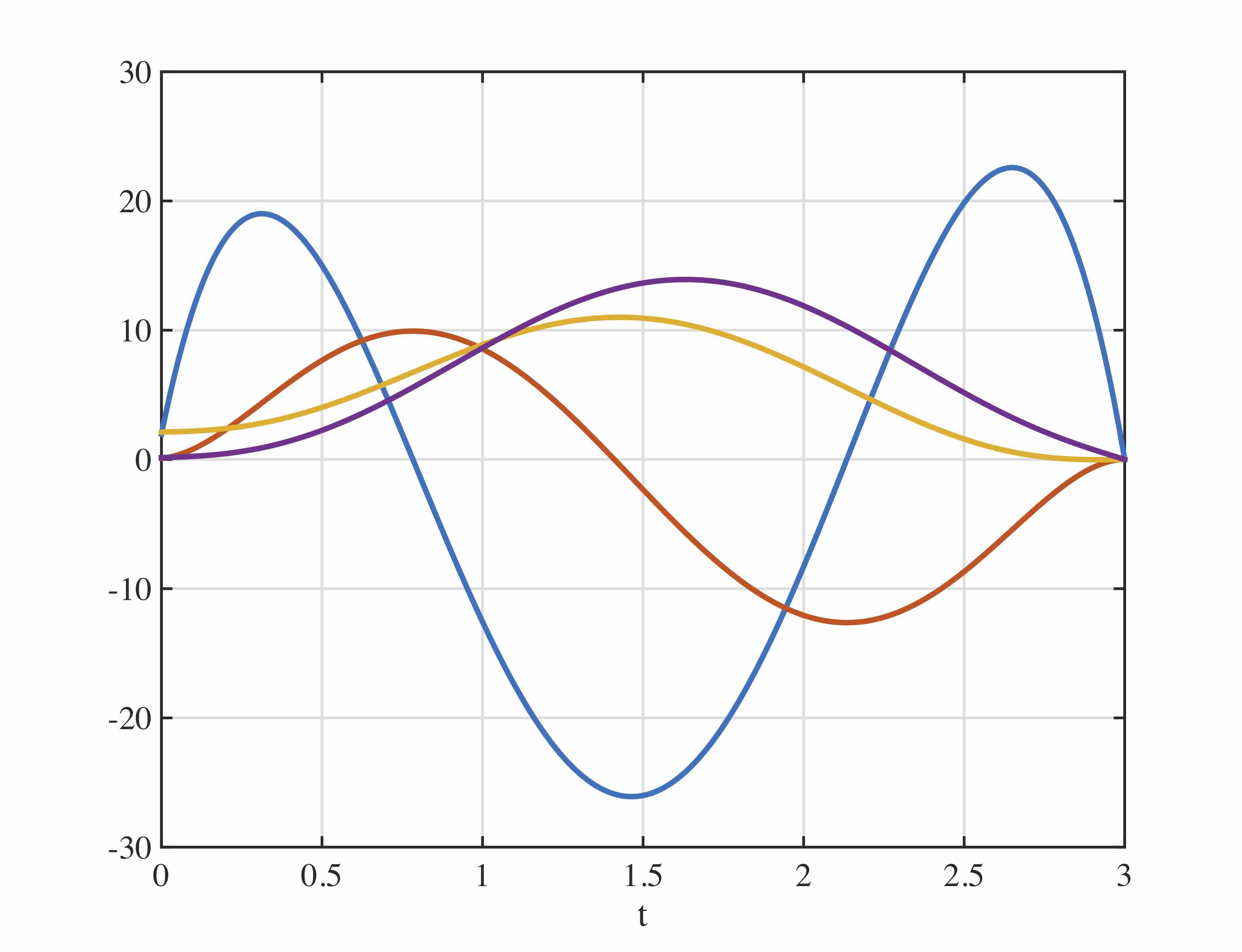
Figure 5: Illustration of the convergence of the system states. The time constant $t_{f}$ is set as $t_{f}=3$.

IV-B Target control in ER, SF and real-life networks.

In this subsection, we test MFTP in Erdos-Renyi (ER) [26] networks and Scale-Free (SF) [27] networks as well as some real-life networks. The reason of choosing ER and SF networks is because both of them preserve quite common properties of a vast number of natural and artificial networks. Figure 6 shows the results in ER networks with $N=1000$ nodes and $\mu$ varying from $\mu=1$ to $\mu=5$, where $\mu$ is the mean degree of the network hereafter. For a given fraction of network nodes selected as target nodes (denoted as $S$), the required minimum number of external control sources for this case is close to the neutral expected fraction of external control sources. That is to say, to control an $f$ fraction of target nodes we need approximately about $fN_{D}$ external control sources, where $N_{D}$ is the minimum number of driver nodes using MM [4] algorithm when $S=V$. As shown in Theorem 4, these external control sources can be located based on MFTP. We would like to note that this conclusion is still valid when SF networks are tested with $\mu=3$, and $\gamma=3$ ($N=1000$) as shown in Figure 7, where $\gamma$ is the tail index of SF networks. However, generally SF networks require more external control sources than ER networks. Because typically a SF network has a much larger portion of low-degree nodes compared to an ER network made up of the same volume of nodes and links. This may lead to significant differences in the external control sources allocation. We have also tested MFTP in a few real life networks (Wiki-Vote [28], Crop-own [29], Circuit-s838 [30] p2p-Gnutella [31] physican-discuss-rev [32], physican-friend-rev [33], celegans [34] and one-mode-char [35]) as shown in Figure 8. It is observed that different network topologies may lead to significant differences when locating the target controllable nodes. Such observations may be important if one want to understand how the structures of the networks affect the target control of real-life networks.

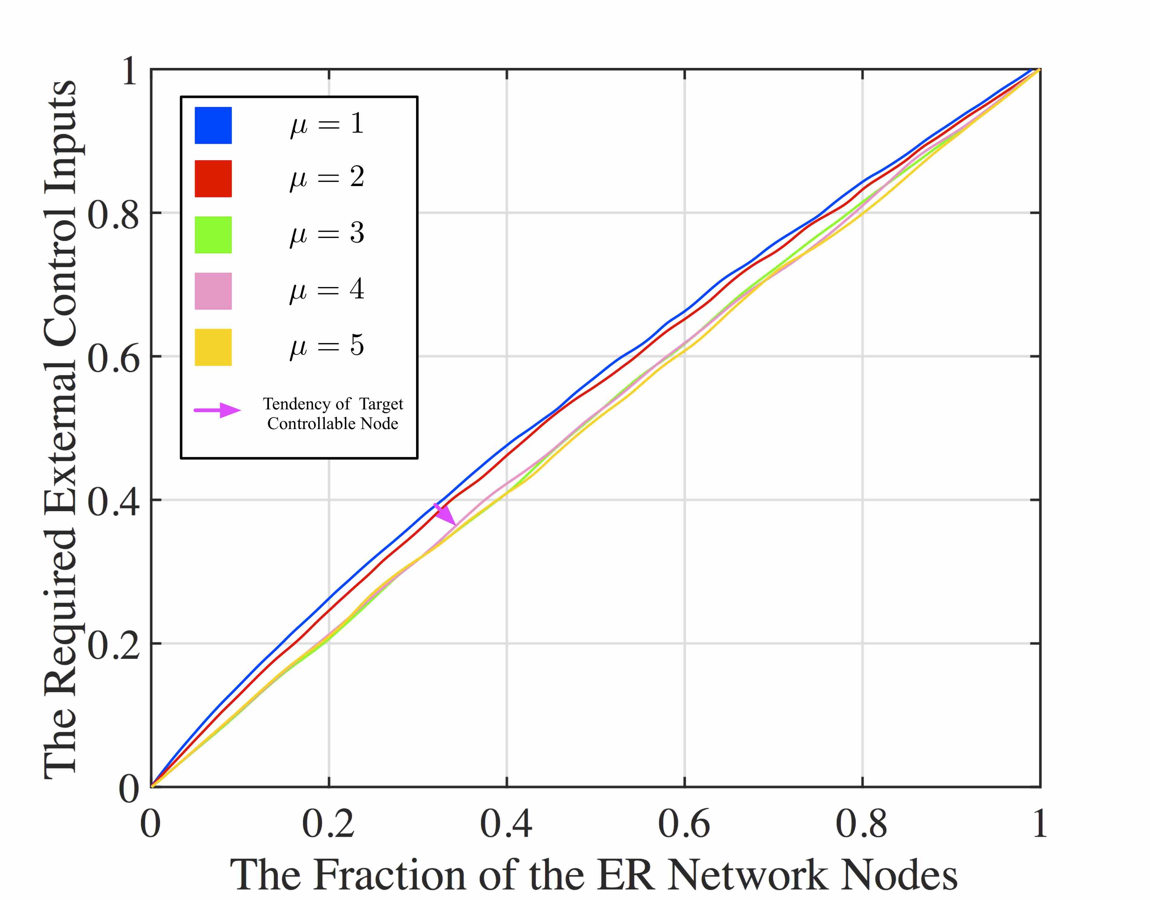
Figure 6: Minimum number of required external control sources in ER networks. The y-axis is normalized by the total minimum number of driver nodes of the whole network, i.e. the y-axis is the ratio ($\frac{n_{D}}{N_{D}}$, where $n_{D}$ is the minimum number of driver nodes of target subset).

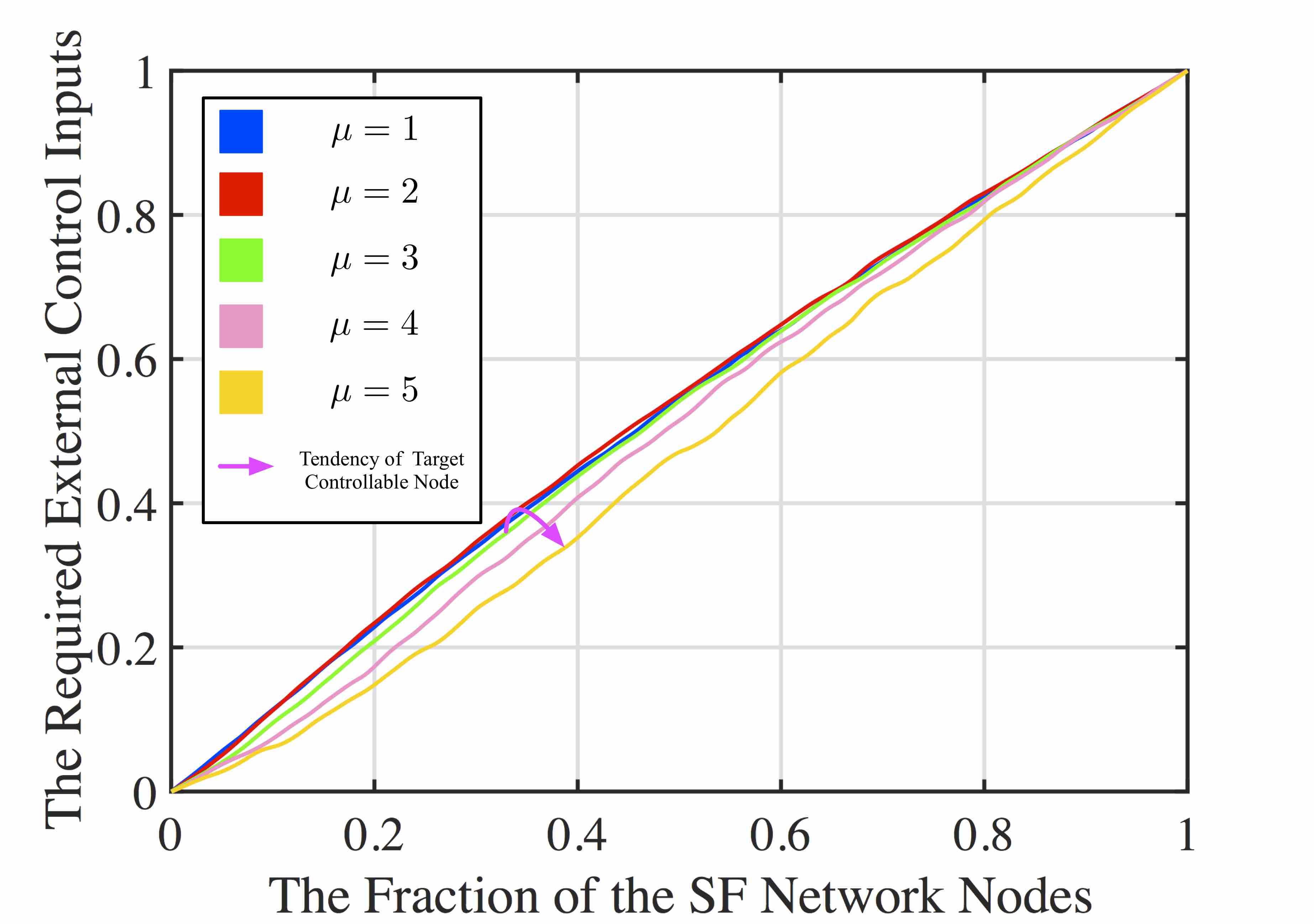
Figure 7: Minimum number of required external control sources in SF networks. The y-axis is normalized by the total minimum number of driver nodes of the whole network, i.e. the y-axis is the ratio ($\frac{n_{D}}{N_{D}}$, where $n_{D}$ is the minimum number of driver nodes of target subset).

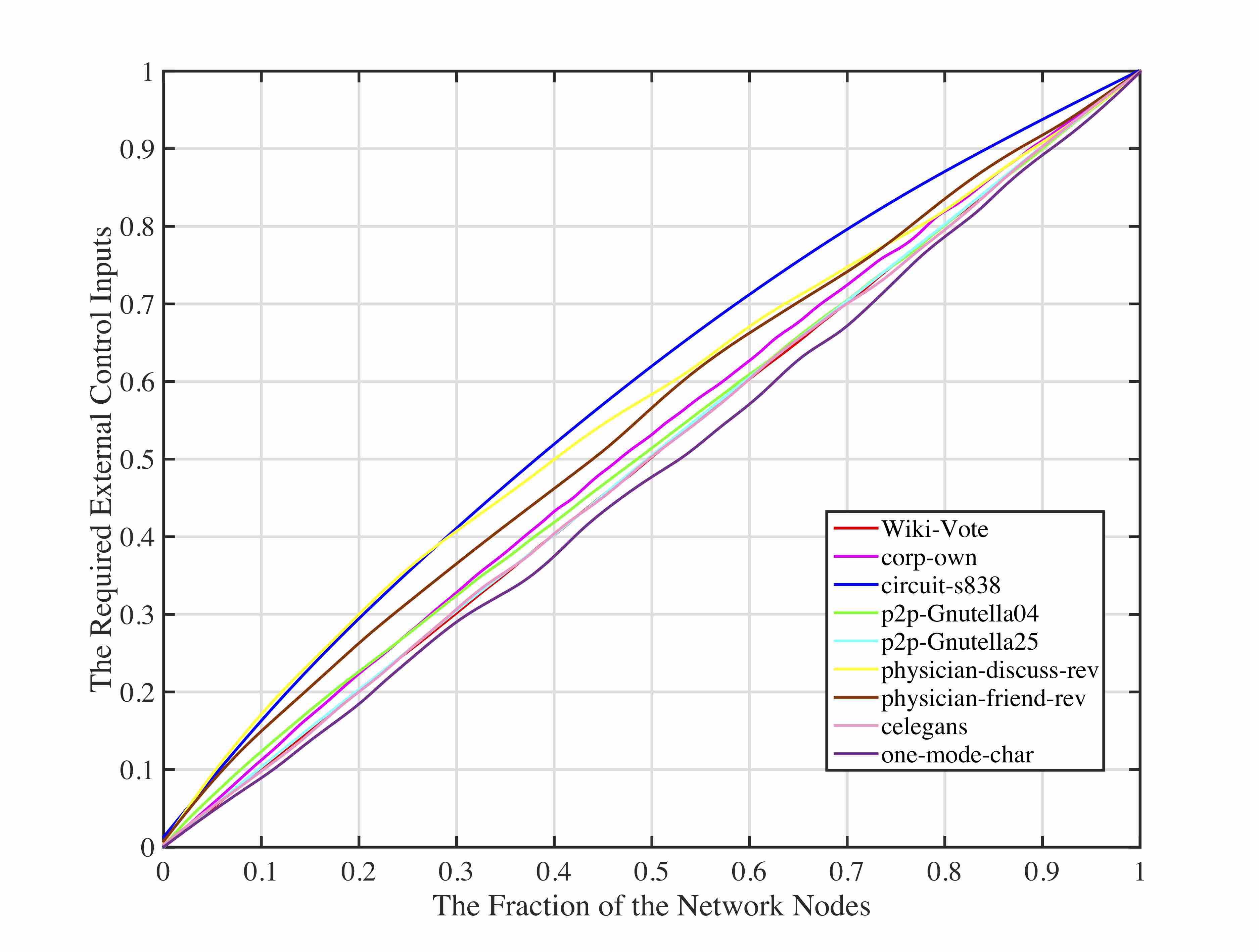
Figure 8: Results in real life networks. The y-axis is normalized by the total minimum number of driver nodes of the whole network, i.e. the y-axis is the ratio ($\frac{n_{D}}{N_{D}}$, where $n_{D}$ is the minimum number of driver nodes of target subset).

V Discussions and Conclusion

In this work, we have solved an open problem regarding how to allocate the minimum number of sources for ensuring the target controllability of a subset of nodes $S$ in real-life networks in which loops are generally exist. The target controllability problem is converted to a maximum flow problem in graph theory under specific constraint conditions. We have rigorously proven the validity of the model transformation. An algorithm termed “maximum flow based target path cover” (MFTP) was proposed to solve the transformed problem. Experimental examples demonstrated the effectiveness of MFTP.

It is shown that the solution of the maximum network flow problem provides strictly the minimum number of control sources for arbitrary directed networks, whether the loops exist or not. By this work, a link from target structural controllability to network flow problems has been established. We anticipate that our work would serve wide applications in target control of real-life complex networks, as well as counter control of various systems which may contribute to enhancing system robustness and resilience. As seen in this work, our model considers only LTI systems and we believe that extending the results to directed networks with nonlinear dynamics light up the way of our future research.

.

Guoqi Li received the B.Eng. degree and M.Eng. degree from Xi’an University of Technology and Xi’an Jiaotong University, P. R. China, in 2004 and 2007, respectively, and Ph.D. degree from Nanyang Technological University, Singapore in 2011. He was a Scientist with Data Storage Institute and Institute of High Performance Computing, Agency for Science, Technology and Research (A*STAR), Singapore, from September 2011 to March 2014. Since March 2014, he has been an Assistant Professor with the Department of Precision Instrument, Tsinghua University, P. R. China. Dr. Li has authored or co-authored more than 80 journal and conference papers. His current research interests include brain-inspired computing, complex systems, machine learning and neuromorphic computing. He has been actively involved in professional services such as serving as an International Technical Program Committee Member and a Track Chair for international conferences. He is an Editorial-Board Member and a Guest Associate Editor for Frontiers in Neuroscience (Neuromorphic Engineering section). He serves as a reviewer for a number of international journals.

Xumin Chen was born in China in 1992. Currently he is a Ph.D. student of Department of Computer Science and Technology in Tsinghua University, P.R.China. His research interests include network representation learning and network mining. He was the main coach of China national team to International Olympiad in Informatics in 2016.

Pei Tang received the bachelor’s degree from Tsinghua University, Beijing, China, in 2010, where he is currently pursuing the Ph.D. degree with the Center for Brain Inspired Computing Research, Department of Precise Instrument. His current research interests include brain inspired computing, complex systems, reinforcement learning, and brain inspired chip design.

Changyun Wen received B.Eng. degree from Xi’an Jiaotong University, China in 1983 and Ph.D. degree from the University of Newcastle, Australia in 1990. From August 1989 to August 1991, he was a Postdoctoral Fellow at University of Adelaide. Since August 1991, he has been with School of EEE, Nanyang Technological University, where he is currently a Full Professor. His main research activities are control systems and applications, intelligent power management system, smart grids, model based online learning and system identification. He is an Associate Editor of a number of journals including Automatica, IEEE Transactions on Industrial Electronics and IEEE Control Systems Magazine. He is the Executive Editor-in-Chief, Journal of Control and Decision. He served the IEEE Transactions on Automatic Control as an Associate Editor from January 2000 to December 2002. He has been actively involved in organizing international conferences playing the roles of General Chair, General Co-Chair, Technical Program Committee Chair, Program Committee Member, General Advisor, Publicity Chair and so on. He received the IES Prestigious Engineering Achievement Award 2005 from the Institution of Engineers, Singapore (IES) in 2005. Dr. Wen is a Fellow of IEEE, a member of IEEE Fellow Committee from 2011 to 2013 and a Distinguished Lecturer of IEEE Control Systems Society from February 2010 to February 2013.

Gaoxi Xiao received the B.S. and M.S. degrees in applied mathematics from Xidian University, Xi’an, China, in 1991 and 1994 respectively. He was an Assistant Lecturer in Xidian University in 1994-1995. In 1998, he received the Ph.D. degree in computing from the Hong Kong Polytechnic University. He was a Postdoctoral Research Fellow in Polytechnic University, Brooklyn, New York in 1999; and a Visiting Scientist in the University of Texas at Dallas in 1999-2001. He joined the School of Electrical and Electronic Engineering, Nanyang Technological University, Singapore, in 2001, where he is now an Associate Professor. His research interests include complex systems and complex networks, communication networks, smart grids, and system resilience and risk management. Dr. Xiao serves/served as an Editor or Guest Editor for IEEE Transactions on Network Science and Engineering, PLOS ONE and Advances in Complex Systems etc., and a TPC member for numerous conferences including IEEE ICC and IEEE GLOBECOM etc.

Luping Shi received the B. S. degree and M. S. degree in Physics from Shandong University, China in 1981 and 1988, respectively, and Ph. D. degree in Physics from University of Cologne, Germany in 1992. He was a post-doctoral fellow at Fraunhofer Institute for Applied Optics and Precision Instrument, Jela, Germany in 1993 and a research fellow in Department of Electronic Engineering, City University of Hong Kong from 1994 to 1996. From 1996 to 2013, he worked in Data Storage Institute (DSI), Singapore as a senior scientist and division manager, and led nonvolatile solid-state memory (NVM), artificial cognitive memory (ACM) and optical storage researches. He is the recipient of the National Technology Award 2004 Singapore, the only one awardee that year. He joined THU, China, as a national distinguished professor and director of Optical Memory National Engineering Research Center in 2013. By integrating 7 departments (Precision Instrument, Computer Science, Electrical Engineering, Microelectronics, Medical School, Automatics, Software School), he established CBICR, THU in 2014, and served as the director. His research interests include brain-inspired computing, neuromorphic engineering, NVM, memristor devices, optical data storage, photonics, etc. Dr. Shi has published more than 150 papers in prestigious journals including Science,Nature Photonics, Advanced Materials, Physical Review Letters, filed and granted more than 10 patents and conducted more than 60 keynote speech or invited talks at many important conferences during last 10 years. Dr. Shi is a SPIE fellow, and general co-chair of the 9th Asia-Pacific Conference on Near-field Optics2013, IEEE NVMTS 2011-2015, East-West Summit on Nanophotonics and Metal Materials 2009 and ODS009. He is a member of the editorial board of Scientific Reports (Nature Publishing Group).

References

- [1] D. J. Watts and S. H. Strogatz, “Collective dynamics of’small-world’networks,” nature, vol. 393, no. 6684, p. 440, 1998.
- [2] S. H. Strogatz, “Exploring complex networks,” nature, vol. 410, no. 6825, p. 268, 2001.
- [3] B. A.-L. Barabási and E. Bonabeau, “Scale-free,” Scientific American, vol. 288, no. 5, pp. 50–59, 2003.
- [4] Y.-Y. Liu, J.-J. Slotine, and A.-L. Barabási, “Controllability of complex networks,” nature, vol. 473, no. 7346, p. 167, 2011.
- [5] J. Ruths and D. Ruths, “Control profiles of complex networks,” Science, vol. 343, no. 6177, pp. 1373–1376, 2014.
- [6] K. Murota, Matrices and matroids for systems analysis. Springer Science & Business Media, 2009, vol. 20.
- [7] Y.-Y. Liu and A.-L. Barabási, “Control principles of complex systems,” Reviews of Modern Physics, vol. 88, no. 3, p. 035006, 2016.
- [8] C. Commault, J.-M. Dion, and J. W. van der Woude, “Characterization of generic properties of linear structured systems for efficient computations,” Kybernetika, vol. 38, no. 5, pp. 503–520, 2002.
- [9] I. Klickstein, A. Shirin, and F. Sorrentino, “Energy scaling of targeted optimal control of complex networks,” Nature Communications, vol. 8, 2017.
- [10] J. Gao, Y.-Y. Liu, R. M. D’souza, and A.-L. Barabási, “Target control of complex networks,” Nature communications, vol. 5, p. 5415, 2014.
- [11] N. Monshizadeh, K. Camlibel, and H. Trentelman, “Strong targeted controllability of dynamical networks,” in Decision and Control (CDC), 2015 IEEE 54th Annual Conference on. IEEE, 2015, pp. 4782–4787.
- [12] H. J. van Waarde, M. K. Camlibel, and H. L. Trentelman, “A distance-based approach to strong target control of dynamical networks,” IEEE Transactions on Automatic Control, 2017.
- [13] E. W. Dijkstra, “A note on two problems in connexion with graphs,” Numerische mathematik, vol. 1, no. 1, pp. 269–271, 1959.
- [14] A. Olshevsky, “Minimal controllability problems,” IEEE Transactions on Control of Network Systems, vol. 1, no. 3, pp. 249–258, 2014.
- [15] A. Sharma, C. Cinti, and E. Capobianco, “Multitype network-guided target controllability in phenotypically characterized osteosarcoma: Role of tumor microenvironment,” Frontiers in immunology, vol. 8, p. 918, 2017.
- [16] W.-F. Guo, S.-W. Zhang, Q.-Q. Shi, C.-M. Zhang, T. Zeng, and L. Chen, “A novel algorithm for finding optimal driver nodes to target control complex networks and its applications for drug targets identification,” BMC Genomics, vol. 19, no. 1, p. 924, 2018.
- [17] C.-T. Lin, “Structural controllability,” IEEE Transactions on Automatic Control, vol. 19, no. 3, pp. 201–208, 1974.
- [18] L. Blackhall and D. J. Hill, “On the structural controllability of networks of linear systems,” IFAC Proceedings Volumes, vol. 43, no. 19, pp. 245–250, 2010.
- [19] J. L. Gross and J. Yellen, Graph theory and its applications. CRC press, 2005.
- [20] ——, Handbook of graph theory. CRC press, 2004.
- [21] R. Balakrishnan and K. Ranganathan, A textbook of graph theory. Springer Science & Business Media, 2012.
- [22] J. Kleinberg and E. Tardos, Algorithm design. Pearson Education India, 2006.
- [23] E. Dinits, “Algorithms for solution of a problem of maximum flow in a network with power estimation,” Soviet Math. Cokl., vol. 11, pp. 1277–1280, 1970.
- [24] Y. Dinitz, “Dinitz’algorithm: The original version and even’s version,” in Theoretical computer science. Springer, 2006, pp. 218–240.
- [25] S. Even and R. E. Tarjan, “Network flow and testing graph connectivity,” SIAM journal on computing, vol. 4, no. 4, pp. 507–518, 1975.
- [26] P. Erdos and A. Rényi, “On the evolution of random graphs,” Publ. Math. Inst. Hung. Acad. Sci, vol. 5, no. 1, pp. 17–60, 1960.
- [27] R. Albert and A.-L. Barabási, “Statistical mechanics of complex networks,” Reviews of modern physics, vol. 74, no. 1, p. 47, 2002.
- [28] J. Leskovec, D. Huttenlocher, and J. Kleinberg, “Signed networks in social media,” in Proceedings of the SIGCHI conference on human factors in computing systems. ACM, 2010, pp. 1361–1370.
- [29] K. Norlen, G. Lucas, M. Gebbie, and J. Chuang, “Eva: Extraction, visualization and analysis of the telecommunications and media ownership network,” in Proceedings of International Telecommunications Society 14th Biennial Conference (ITS2002), Seoul Korea, 2002.
- [30] R. Milo, S. Itzkovitz, N. Kashtan, R. Levitt, S. Shen-Orr, I. Ayzenshtat, M. Sheffer, and U. Alon, “Superfamilies of evolved and designed networks,” Science, vol. 303, no. 5663, pp. 1538–1542, 2004.
- [31] M. Ripeanu and I. Foster, “Mapping the gnutella network: Macroscopic properties of large-scale peer-to-peer systems,” in International Workshop on Peer-to-Peer Systems. Springer, 2002, pp. 85–93.
- [32] J. Leskovec, D. Huttenlocher, and J. Kleinberg, “Predicting positive and negative links in online social networks,” in Proceedings of the 19th international conference on World wide web. ACM, 2010, pp. 641–650.
- [33] J. Leskovec, K. J. Lang, A. Dasgupta, and M. W. Mahoney, “Community structure in large networks: Natural cluster sizes and the absence of large well-defined clusters,” Internet Mathematics, vol. 6, no. 1, pp. 29–123, 2009.
- [34] M. P. Young, “The organization of neural systems in the primate cerebral cortex,” Proceedings of the Royal Society of London B: Biological Sciences, vol. 252, no. 1333, pp. 13–18, 1993.
- [35] T. Opsahl and P. Panzarasa, “Clustering in weighted networks,” Social networks, vol. 31, no. 2, pp. 155–163, 2009.