Kinetic energy spectra and flux in turbulent phase-separating symmetric binary-fluid mixtures

Abstract

We conduct direct numerical simulation (DNS) of the Cahn-Hilliard-Navier-Stokes (CHNS) equations to investigate the statistical properties of the turbulent phase-separating symmetric binary-fluid mixture. Turbulence causes an arrest of the phase-separation which leads to the formation of a statistically steady emulsion. We characterize turbulent velocity fluctuations in an emulsion for different values of the Reynolds number and the Weber number. Our scale-by-scale kinetic energy budget analysis shows that the interfacial terms in the CHNS provide an alternate route for the kinetic energy transfer. By studying the probability distribution function (PDF) of the energy dissipation rate, the vorticity magnitude, and the joint-PDF of the velocity-gradient invariants we show that the statistics of the turbulent fluctuations do not change with the Weber number.

1 Introduction

Below the consolute temperature, a symmetric binary-mixture in spatially homogeneous composition spontaneously phase separates forming domains of individual phases via the process of spinodal decomposition, see e.g. the books Chaikin and Lubensky (1998); Goldenfeld (2005). During the dynamics, individual domains merge and coarsen to form even larger domain until a final configuration is reached wherein two single-component domains separated by an interface is formed. The exact mechanism of domain growth depends on the interplay of viscous, inertial, and surface tension forces (Lifshitz and Slyozov, 1961; Siggia, 1979; Furukawa, 1985; Bray, 1994; Kendon, 2000; Kendon et al., 2001; Puri, 2009; Datt et al., 2015; Cates and Tjhung, 2018).

Presence of an external stirring such as shear or turbulent mixing counteracts the phase separation by breaking the coarsening domains to form a statistically stationary emulsion. In presence of an external shear (with rate $\dot{\gamma}$), the size of a typical domain $D$ in an emulsion state can be estimated by the balance of shear stress $\eta\dot{\gamma}$ with the capillary force density $\sigma/D$ which gives $D\sim\sigma/{\eta\dot{\gamma}}$ (Hashimoto et al. (1995)). Here $\eta$ is the dynamic viscosity of the emulsion and $\sigma$ its surface tension. Although both experiments (Onuki, 2002) and numerical simulations (Stansell et al., 2006; Stratford et al., 2007; Cates and Tjhung, 2018) confirm formation of an emulsion state, the domain size shows different scaling with shear rate in the direction perpendicular and parallel to the shear (Stansell et al., 2006; Stratford et al., 2007; Cates and Tjhung, 2018).

The situation is much more tractable when the binary-fluid mixture emulsion is formed by an external stirring that generates homogeneous, isotropic turbulence (HIT). The average domain size $D$ of such an emulsion can be estimated by a balance of inertial stress [$\rho(\delta_{D}U)^{2}$] with the capillary force density ($\sigma/D$) (Hinze, 1955), where $\delta_{D}U$ is the typical velocity difference across the domain. Using $\delta_{D}U\sim D^{1/3}\epsilon_{\nu}^{1/3}$ (Kolmogorov, 1941; Frisch, 1996), where $\epsilon$ is the energy dissipation rate, provides an estimate for the average domain size as $D\sim(\rho/\sigma)^{-3/5}\epsilon^{-2/5}$. Early experiments (Pine et al., 1984; Easwar, 1992) indicated an arrest of the phase separation process in presence of HIT. This was theoretically understood by using eddy diffusivity arguments by Aronovitz and Nelson (1984). However, only recent numerical investigations using a multicomponent Lattice-Boltzmann method in three-dimensions (Perlekar et al., 2014) and direct numerical simulations (DNSs) of Cahn-Hilliard-Navier-Stokes equations in two-dimensions (Berti et al., 2005; Fan et al., 2016; Perlekar et al., 2017; Fan et al., 2018) have been able to study emulsification by turbulence in symmetric binary-fluid mixtures. Surprisingly, unlike shear flows, here numerically calculated domain size is in excellent agreement with Hinze’s prediction in both two- and three-dimensions.

It is apriori unclear whether turbulence in binary-fluid mixtures is similar or different than a single-component Newtonian fluid as only a small fraction of the volume is occupied by the emulsion interfaces. In two-dimensions, Perlekar et al. (2017) show that the inverse energy cascade and the corresponding energy flux gets blocked at a wave-number corresponding to the domain size $D$. In three-dimensions, numerical investigations (Kendon et al., 2001; Perlekar et al., 2014) show that for a binary-fluid mixture energy content in the inertial range is suppressed in comparison to a single-component fluid at the same Reynolds number. However, an understanding of the underlying energy transfer mechanisms in three-dimensions remains unclear.

In this paper, we conduct DNSs to investigate the energy transfer mechanisms and the statistical properties of the velocity fluctuations in a stirred three-dimensional symmetric binary fluid mixture. Our main findings are: $(i)$ External stirring arrests phase-separation (coarsening); $(ii)$ Our scale-by-scale analysis reveals that interfaces provide an alternate route for energy transfer and dissipation; $(iii)$ For same Reynolds number, a single-component fluid and a binary-fluid mixture have same small-scale statistics.

The rest of the paper is organised as follows. We present the equations and the numerical method that we use in Sec. 2. In Sec 3.1-3.3 we derive the equations for the total energy, the scale-by-scale kinetic energy budget, and present our numerical findings. In Sec. 4 we investigate the small-scale statistics of the vorticity magnitude and the energy dissipation rate. We conclude in Section 5.

2 Equations and Direct Numerical Simulation (DNS)

We model symmetric binary-fluid mixture by using the Navier-Stokes-Cahn-Hilliard (NSCH) or Model-H (Cahn, 1968; Hohenburg and Halperin, 1977) equations

$$\rho(\partial_{t}+\bm{u}\cdot\nabla){\bm{u}} = \eta\nabla^{2}{\bm{u}}-\nabla P+\Lambda\phi\nabla\nabla^{2}\phi+f,$$ (1)

$$(\partial_{t}+{\bm{u}}\cdot\nabla){\phi} = M\nabla^{2}\mu,$$ (2)

$$\mu \equiv \Lambda\left(\frac{-\phi+\phi^{3}}{\xi^{2}}-\nabla^{2}\phi\right),~{}{\rm{and}}$$

$$\nabla\cdot{\bm{u}} = 0.$$

Here ${\phi},{\bm{u}}$, and $P$ are the Cahn-Hilliard order-parameter, the velocity, and the pressure field at position ${\bm{x}}$ and time $t$, $\eta$ is the dynamic viscosity, $\rho$ is the density, the kinematic viscosity $\nu\equiv\eta/\rho$, $M$ is the mobility, $\xi$ controls the width of the interface between the two phases, $\Lambda$ is the mixing energy density, the order-parameter diffusivity $\kappa=M\Lambda/\xi^{2}$, the surface tension $\sigma=2\sqrt{2}/3(\Lambda/\xi)$, and ${\bm{f}}$ is the external forcing that generates turbulence. The order parameter takes positive values in one phase and negative in the other. For simplicity, we assume the density ($\rho=1$), the viscosity $\eta$, and the mobility $M$ to be independent of $\phi$ and same for the two phases . The local vorticity ${\bm{\omega}}\equiv\nabla\times{\bm{u}}$. Note that the pressure $P$ also contains contributions due to longitudinal terms in $\phi$. We use a cubic domain with each side of length ${\cal L}=2\pi$ and discretize it with $N^{3}$ collocation points. We employ periodic boundary conditions. Eqs. (1) and (2) are numerically integrated using a pseudo-spectral method with $1/2$-dealiasing and time marching is done using an exponential Adams-Bashforth scheme (Cox and Matthews, 2002). A large-scale forcing $\hat{\bm{f}}_{\bm{k}}=f_{0}\hat{\bm{u}}_{k}/\sum_{k=1,2}|{\bm{u}}_{k}|^{2}$, where the caret indicates Fourier transform, with $|{\bm{k}}|\leq 2$ ensures constant energy injection rate $\epsilon_{inj}$.

3 Results

The energy injection based Reynolds number $\mbox{Re}\equiv\sqrt{\epsilon_{inj}^{1/3}{\cal L}^{4/3}/\nu}$ and Weber number $\mbox{We}\equiv\rho\epsilon_{inj}^{2/3}{\cal L}^{5/3}/\sigma$ characterise the turbulence intensity of the flow. Table 1 summarises the parameters that we use. All the simulations were time-integrated up to $t=100T_{\cal L}$ ($T_{\cal L}\equiv\epsilon_{inj}^{1/3}{\cal L}^{-2/3}$). We collect the statistics after a steady-state is attained $(t>40T_{\cal L})$.

	$N$	$\nu$	$\xi(\times 10^{-2})$	$\kappa$	$\sigma(\times 10^{-1})$	Re	We	$\epsilon_{inj}$	$\epsilon_{\nu}(\times 10^{-1})$	$\epsilon_{\mu}(\times 10^{-1})$
NS1	$256$	$5\cdot 10^{-3}$	$-$	$-$	$-$	$65$	$-$	$0.05$	$0.05$	$-$
SP11	$256$	$5\cdot 10^{-3}$	$1.88$	$10^{-2}$	$2.51$	$65$	$11.6$	$0.05$	$0.33$	$0.18$
SP12	$256$	$5\cdot 10^{-3}$	$1.88$	$10^{-2}$	$0.63$	$65$	$46.4$	$0.05$	$0.23$	$0.28$
SP13	$256$	$5\cdot 10^{-3}$	$1.88$	$10^{-2}$	$0.25$	$65$	$116.2$	$0.05$	$0.23$	$0.27$
NS2	$512$	$5\cdot 10^{-3}$	$-$	$-$	$-$	$96$	$-$	$0.5$	$0.5$	$-$
SP21	$512$	$5\cdot 10^{-3}$	$3.76$	$10^{-2}$	$5.02$	$96$	$26.9$	$0.5$	$3.10$	$1.90$
SP22	$512$	$5\cdot 10^{-3}$	$3.76$	$10^{-2}$	$3.76$	$96$	$35.9$	$0.5$	$2.90$	$2.15$
SP23	$512$	$5\cdot 10^{-3}$	$3.76$	$10^{-2}$	$2.50$	$96$	$53.9$	$0.5$	$2.67$	$2.35$
SP24	$512$	$5\cdot 10^{-3}$	$3.76$	$10^{-2}$	$1.25$	$96$	$107.9$	$0.5$	$2.36$	$2.55$

Table 1: Parameters $N,\nu,\xi,\kappa,\sigma,Re,We,\epsilon_{inj},\epsilon_{\nu},\epsilon_{\mu}$ for our binary-fluid DNS SP11-3 and SP21-4. The ${\tt NS}$ runs are the DNS studies conducted for single-component Navier-Stokes fluid with the same $\nu$ and $\epsilon_{inj}$ as the binary-fluid.

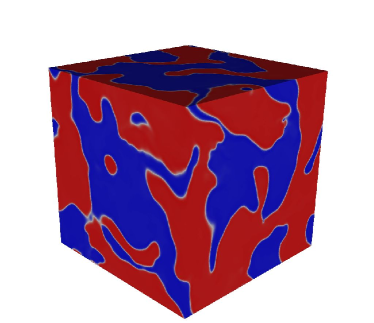
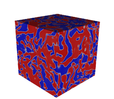
Figure 1: Pseudocolor plot of the order parameter field $\phi$ for $\mbox{Re}=96$, $\mbox{We}=26.9$ (left) and for $\mbox{Re}=96,\mbox{We}=107.9$ (right). Regions with $\phi=1(-1)$ are shown in red (blue). Average domain size decreases with increasing We.

3.1 Domain size and Energy balance

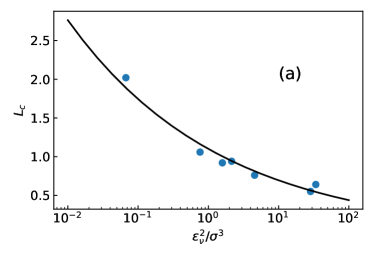
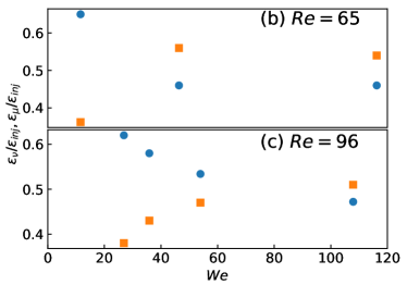
Figure 2: (a) Semilog plot of the domain scale $L_{c}$ versus $\epsilon_{\nu}^{2}/\sigma^{3}$ (blue dots) and its comparison with the Hinze prediction for the domain scale [$D\sim(\epsilon_{\nu}^{2}/\sigma^{3})^{-1/5}$, black line]. (b,c) $\epsilon_{\nu}/\epsilon_{inj}$ (blue circle) and $\epsilon_{\mu}/\epsilon_{inj}$ (orange square) with varying Weber number We for $\mbox{Re}=65$ (runs SP11-13) and $\mbox{Re}=96$ (runs SP21-24).

In Fig. 1 we plot the representative snapshots of the steady-state order-parameter field $\phi$ for our runs ${\tt SP21}$ $(\mbox{Re}=96,\mbox{We}=26.9)$and ${\tt SP24}$ $(\mbox{Re}=96,\mbox{We}=107.9)$. We observe that the domain size in the emulsion decreases with increasing We. From $\phi$, we estimate the average domain size as

$$L_{c}=2\pi\left\langle\frac{\sum_{\bm{k}}|\hat{\phi}_{\bm{k}}|^{2}}{\sum_{\bm{k}}k|\hat{\phi}_{\bm{k}}|^{2}}\right\rangle,$$ (3)

where $k=\sqrt{{\bm{k}}\cdot{\bm{k}}}$ and angular brackets denote time-averaging in the statistically steady-state. In Fig. (2a) we present a consolidated plot of $L_{c}$ versus $\epsilon_{\nu}^{2}/\sigma^{3}$ for different value of Re and We (see Table 1). We find the data to be in good agreement with Hinze’s prediction for the average domain size in an emulsion $D\sim(\rho\epsilon_{\nu}^{2}/\sigma^{3})^{-1/5}$.

We next investigate how much of the energy injected $\epsilon_{inj}$ is dissipated by the viscosity $\epsilon_{\nu}$ and how much is the interfacial contribution $\epsilon_{\mu}$. Using Eq. (1) and Eq. (2), we obtain the following energy balance equation:

$$\begin{split}\partial_{t}\underbrace{\int\frac{|\bm{u}|^{2}}{2}d{\bm{x}}}_{\cal K}+&\partial_{t}\underbrace{\int\frac{\Lambda}{\xi^{2}}\left(-\frac{\phi^{2}}{2}+\frac{\phi^{4}}{4}+\frac{\xi^{2}}{2}|\nabla\phi|^{2}\right)d{\bm{x}}}_{\cal G}\\ &\quad=-\underbrace{\nu\int|\nabla u|^{2}d{\bm{x}}}_{\epsilon_{\nu}}-\underbrace{M\int|\nabla\mu|^{2}d{\bm{x}}}_{\epsilon_{\mu}}+\underbrace{\int{\bm{f}}\cdot{\bm{u}}d{\bm{x}}}_{\epsilon_{inj}}.\end{split}$$ (4)

Here ${\cal K}$ is the kinetic energy, ${\cal G}$ is the free energy of mixing, $\epsilon_{\nu}$ is the viscous energy dissipation, $\epsilon_{\mu}$ is the dissipation because of the chemical potential (interfacial contribution), and $\epsilon_{inj}$ is the energy injected because of the external forcing. In the statistically steady-state, $\langle\epsilon_{inj}\rangle\approx\langle\epsilon_{\nu}\rangle+\langle\epsilon_{\mu}\rangle$. In Fig. (2b,c) we show that for small We, the viscosity is the primary dissipation mechanism $\langle\epsilon_{\nu}\rangle\gg\langle\epsilon_{\mu}\rangle$ whereas, for large We average domain size reduces thereby making the interfacial contribution more dominant $\langle\epsilon_{\mu}\rangle>\langle\epsilon_{\nu}\rangle$.

3.2 Energy spectrum

The steady-state energy spectrum is defined as (Vincent and Meneguzzi, 1991)

$$E(k)=\frac{1}{2}\left\langle\sum_{k-1/2<k^{\prime}\leq k+1/2}|\hat{\bm{u}}_{\bm{k}^{\prime}}|^{2}\right\rangle.$$ (5)

For high Reynolds number single-component flows, $E(k)\sim k^{-5/3}$ in the inertial range (Kolmogorov, 1941; Frisch, 1996). The energy spectrum obtained from our DNS run ${\tt NS1}$ and ${\tt NS2}$ shows half a decade of scaling for $\mbox{Re}=65$ and nearly a decade of scaling for $\mbox{Re}=96$ [see Fig. (3)]. For the same Reynolds number, the inertial range energy spectrum is suppressed for binary-fluid mixtures for $k<2\pi/L_{c}$. For scales smaller than the average domain size of the emulsion $k>2\pi/L_{c}$, the energy spectrum follows its single-component counterpart. Our high-$\mbox{Re}=96$, high-$\mbox{We}=107.9$ run indicate that Kolmogorov scaling is recovered for $k\ll 2\pi/L_{c}$. Numerical simulations with large scale-separation and much higher spatial resolutions are required to investigate the recovery of Kolmogorov scaling for $2\pi/\ell_{inj}\gg k\gg 2\pi/L_{c}$.

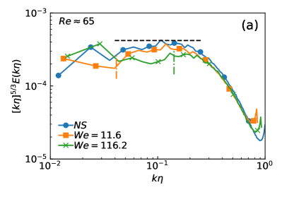
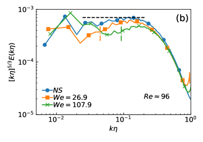
Figure 3: Energy spectrum for (a) $\mbox{Re}=65$ and (b) $\mbox{Re}=96$ for different values of We. The horizontal dashed line indicate Kolmogorov scaling and the vertical dash-dot indicate the wave-number corresponding to the average domain size $2\pi/L_{c}$ in the emulsion.

3.3 Scale-by-scale Kinetic Energy budget

To investigate how the kinetic energy is distributed upto a given length scale $\ell$ (or a corresponding wave-number $k=2\pi/\ell$), we now derive the scale-by-scale energy budget equation. By multiplying the Fourier transformed Eq. (1) with $\hat{\bm{u}}_{-\bm{k}}$, summing up contributions upto wave-number $k$, and then averaging over statistically-steady state we obtain

$$\Pi(k)=-{\cal D}(k)-\Pi^{\phi}(k)+{\cal F}(k).$$ (6)

Here $\Pi(k)\equiv\langle\Re[\sum_{|{\bm{m}}|\leq k}\hat{{\bm{u}}}_{\bm{m}}\cdot\widehat{(\bm{u}\cdot\nabla{\bm{u}})}_{-\bm{m}}]\rangle$ is the energy flux, $\Pi^{\phi}\equiv\Lambda\langle\Re[\sum_{|{\bm{m}}|\leq k}\hat{{\bm{u}}}_{\bm{m}}\cdot\widehat{(\phi\nabla\nabla^{2}\phi)}_{-\bm{m}}]\rangle$ is the cumulative flux of $(\nabla\phi)^{2}$, ${\cal E}(k)\equiv\sum_{m\leq k}E(m)$ is the cumulative energy upto $k$, ${\cal D}(k)\equiv\nu\sum_{m\leq k}m^{2}E(m)$ is the cumulative dissipation upto wave-number $k$, and ${\cal F}(k)\equiv\langle\sum_{|{\bm{m}}|\leq k}\Re[{\bm{u}}_{-\bm{m}}{\bm{f}}_{\bm{m}}]\rangle$ is the cumulative energy injected. In statistically steady state the left hand size is zero and $\Pi(k)={\cal D}(k)-\Pi^{\phi}(k)+{\cal F}(k)$. When $K=2\pi/{\cal L}$, $\Pi=0,{\cal D}=\epsilon_{\nu},\Pi^{\phi}=\epsilon_{\mu},$ and ${\cal F}=\epsilon_{inj}$.

The plot in Fig. (4a,b) shows the scale-by-scale energy budget for $\mbox{Re}=65$ and $\mbox{Re}=96$ for a single-component fluid. The energy is injected at large-scales by forcing ${\cal F}(k)$ and is dissipated by viscosity at small-scales. The Navier-Stokes nonlinearity transfers the kinetic energy in the inertial range while keeping its flux $\Pi(k)$ constant. For our high $\mbox{Re}=96$ run ${\tt NS2}$, we observe a nearly constant $\Pi(k)\sim\epsilon_{inj}$ for $2\leq k\leq 10$ which manifests as an extended inertial range in the energy spectrum [see Fig. (3b)].

We now show that for the binary fluid case, the presence of emulsion domains dramatically alter the energy transfer mechanism. Firstly, for small We, we note that the viscous dissipation $\epsilon_{\nu}\equiv{\cal D}(2\pi/{\cal L})$ is larger than the interfacial dissipation $\epsilon_{\mu}\equiv\Pi^{\phi}(2\pi/{\cal L})$ [Fig. (4b,d)] whereas it is the opposite for high We [Fig. (4e,f)]. Secondly, the interfacial flux $\Pi^{\phi}(K)$ first increases up to a wave-number corresponding to the arrest scale $k_{c}\approx 2\pi/L_{c}$. After $k>k_{c}$, $\Pi^{\phi}(k)$ decreases until for large $k$ where it is equal to $\epsilon_{\mu}$. This indicates that the interface undulations absorb kinetic energy $\sim\Pi^{\phi}(k_{c})$ from large scales. However only part of it, $\epsilon_{\mu}$, is dissipated and the excess energy $\sim\Pi^{\phi}(k_{c})-\epsilon_{\mu}$ is redistributed among wave-numbers $k>k_{c}$. Finally, the contribution because of the kinetic energy flux $\Pi(K)$ is nearly halved in comparison to its single-component fluid counterpart. For $k<k_{c}$ we find that $\Pi(k)$ decreases with increasing $k$. For our high $\mbox{Re}=96$ runs we find a small range where $\Pi(k)\sim\rm{constant}$ after which it again decreases. This is consistent our earlier observation that for binary-fluid Kolmogorov-scaling in the energy spectrum is recovered for $k>2\pi/L_{c}$ [see Fig. (3)] . Thus presence of interface opens up an additional mechanism to transfer kinetic energy from large-scales to scales smaller than the average size of a domain in the emulsion.

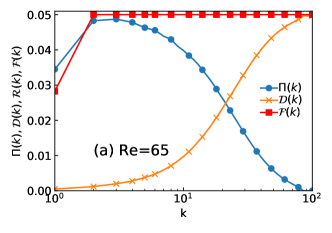
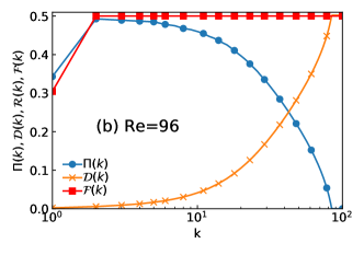
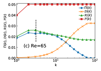
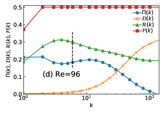
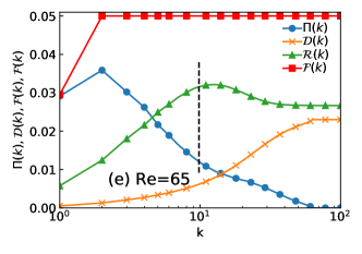
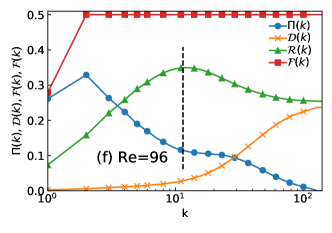
Figure 4: (Top panel) Energy flux for (a) $\mbox{We}\mbox{Re}=65$ (run NS1), (b) $\mbox{Re}=96$ (run NS2), (c) $We\approx 11.6,\mbox{Re}\approx 65$ (run SP11), (d) $We\approx 26.9,\mbox{Re}\approx 96$ (run SP21), (e) $We\approx 116.2,\mbox{Re}\approx 65$ (run SP13), and (f) $We\approx 107.9,\mbox{Re}\approx 96$ (run SP24). The dashed vertical line indicate the wave-number corresponding to the average domain size $2\pi/L_{c}$.

4 Small-scale structures

We now investigate whether the different kinetic energy transfer mechanism in binary-fluid turbulence also alter the small-scale structures. In Fig. (5a,b) we plot the statistics of the local viscous energy-dissipation $\epsilon_{loc}=\sum_{i,j}(\partial_{i}u_{j}+\partial_{j}u_{i})^{2}/2$ and the magnitude of the vorticity field $|{\bm{\omega}}|=\sqrt{{\bm{\omega}}\cdot{\bm{\omega}}}$ for a binary-fluid mixture and compare it with a single-component fluid at the same Re. We observe a reduction in the events with large values of $\epsilon_{loc}$ and $|{\bm{\omega}}|$ on increasing the We. However, the PDFs overlap when normalised by their standard deviations. Thus the small-scale statistics remains the same as that of a single-component turbulent fluid.

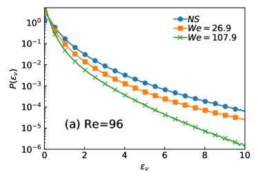
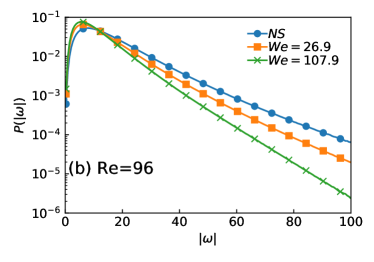
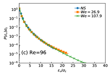
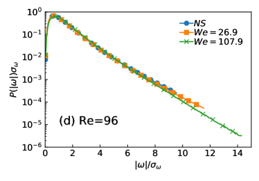
Figure 5: (a,b) Probability distribution function (PDF) of the energy dissipation rate $P(\epsilon_{\nu})$ versus $\epsilon_{\nu}$ and the magnitude of the vorticity $P(|\omega|)$ versus $|\omega|$ for different $We$. (c,d) Normalised PDFs $P(\epsilon_{\nu})\sigma_{\epsilon}$ and $P(|\omega|)$ for different $We$. We fix $\mbox{Re}=96$ (runs SP21, SP24). For comparison we also plot the corresponding PDF for the pure fluid (run NS2).

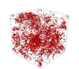
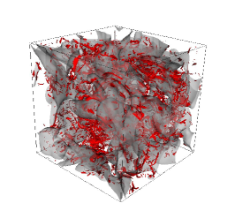
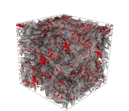
Figure 6: Representative steady state iso-contour plots of the vorticity magnitude $|\omega|$ for $|\omega|=\bar{|\omega|}+6\sigma_{\omega}$. (Left) Pure fluid (run ${\tt NS2}$), and a turbulent binary mixture with $\mbox{We}=26.9$ (center, run ${\tt SP21}$) and $\mbox{We}=107.9$ (Right, run ${\tt SP22}$). For the binary mixture plots we also overlay the iso-contour of the order parameter $\phi$ for $\phi=0$ to highlight the interface.

To investigate the flow structures, in Fig. 6 we plot the iso-vorticity contours for a turbulent binary mixture as well as turbulence in pure fluid and overlay the $\phi=0$ contours on them to highlight the emulsion domains. For the single-component fluid, consistent with earlier studies (Pandit et al., 2009; Ishihara et al., 2009), we observe tubular structures. For the case of binary mixture, as shown earlier, smaller domains (more interfacial area) are formed as we increase We. Also, near the interfacial region vorticity appears to be concentrated. Thus the interface undulations also generate flow structures whose statistics are similar to that of turbulence in a single-component fluid.

The local flow structures as observed by a Lagrangian fluid parcel in a turbulent flow can be quantified by the invariants $R\equiv-\operatorname{Tr}(A^{2})/2$ and $Q\equiv-\operatorname{Tr}(A^{3})/3$ of the velocity gradient tensor $A\equiv\nabla{\bm{u}}$ (Perry and Chong, 1987; Cantwell, 1992). The joint PDF $P(R,Q)$ provides an understanding of the typical structures encountered in a turbulent flow. The discriminant $D\equiv 27Q^{3}/4+R^{2}$ demarcates the regions dominated by vortices ($D>0$) with those that are dominated by strain ($D<0$). To quantify whether the structures formed in pure fluid turbulence are similar or different than a turbulent binary mixture, in Fig. (7) we plot the joint PDF $P(R^{*},Q^{*})$ for the pure fluid turbulence as well as binary fluid turbulence with ${\mbox{Re}=96}$ and ${\mbox{We}=26.9,107.9}$. Although the qualitative features remain the same we observe a small but systematic shrinkage of the iso-contour lines with increasing We.

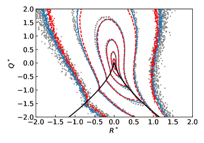
Figure 7: Contour plots of the joint PDF $P(R^{*},Q^{*})$ for pure fluid turbulence [gray dots, run ${\tt NS2}$], and binary-fluid turbulence with $\mbox{We}=26.9$ [blue line, run ${\tt SP21}$], $\mbox{We}=107.9$ [red dashed line, run ${\tt SP24}$]. Here $R^{*}=\nu^{3/2}R/\epsilon_{\nu}^{3/2}$ and $Q^{*}=\nu Q/\epsilon_{\nu}$. The black curve is the $D=0$ line that demarcates regions with vortical $D>0$ or strain $D<0$ dominated flow structures.

5 Conclusions

We investigated turbulence in a stirred phase-separated symmetric binary-fluid mixture. Our study reveals that external stirring leads to the formation of a statistically steady emulsion. Hinze scale provides an estimate for the average domain size. For a binary-fluid mixture, in comparison to a single-component fluid, kinetic energy content is suppressed. We show that this is because the presence of interfaces opens up an alternate kinetic energy transfer mechanism. Emulsion domains absorb kinetic energy up to Hinze scale, dissipate part of it and redistribute the rest to small scales. Surprisingly, even with an alternate energy transfer mechanism, we do not find any qualitative change in the statistics of small-scale structures.

Our results have striking similarity with those of polymeric turbulence (Perlekar et al., 2006, 2010; Valente et al., 2014). There also the presence of polymers modifies the energy transfer in the inertial range. The similarity could be attributed to a close correspondence of the NSCH equations, and the equations for uniaxial polymers (Balkovsky et al., 2001). However, a crucial difference is that the typical size of the polymer is in the dissipation range and they are homogeneously distributed throughout the flow. Whereas the size of binary-fluid domains lie within the inertial range (Aronovitz and Nelson, 1984; Perlekar et al., 2014; Fan et al., 2016).

Acknowledgements
We thank M.M. Bandi, M. Barma, D. Mitra, and F. Toschi for their comments and suggestions.

References

- Aronovitz and Nelson (1984) J. A. Aronovitz and D. R. Nelson. Turbulence in phase-separating binary mixtures. Phys. Rev. A, 29:2012, 1984.
- Balkovsky et al. (2001) E. Balkovsky, A. Fouxon, and V. Lebedev. Turbulence in polymer solutions. Phys. Rev. E, 64:056301, 2001.
- Berti et al. (2005) S. Berti, G. Boffetta, M. Cencini, and A. Vulpiani. Turbulence and coarsening in active and passive binary mixtures. Phys. Rev. Lett., 95:224501, 2005.
- Bray (1994) A. J. Bray. Theory of phase-ordering kinetics. Adv. Phys., 43:357, 1994.
- Cahn (1968) J. Cahn. Spinodal decomposition. Trans. Metall. Soc. AIME, 242:166, 1968.
- Cantwell (1992) B.J. Cantwell. Exact solution of a restricted euler equation for the velocity gradient tensor. Phys. Fluids A, 4:782, 1992.
- Cates and Tjhung (2018) M. E. Cates and E. Tjhung. Theories of binary fluid mixtures: from phase-separation kinetics to active emulsions. J. Fluid Mech., 836:1, 2018.
- Chaikin and Lubensky (1998) P.M. Chaikin and T.C. Lubensky. Principles of condensed matter physics. Cambridge, Cambridge University Press, UK, 1998.
- Cox and Matthews (2002) S. M. Cox and P. C. Matthews. Exponential time differencing for stiff systems. Journal of Computational Physics, 176:430, 2002.
- Datt et al. (2015) C. Datt, S. P. Thampi, and R. Govindarajan. Morphological evolution of domains in spinodal decomposition. Phys. Rev. E, 91:010101, 2015.
- Easwar (1992) N. Easwar. Effect of continuous stirring on off-critical and critical samples of a phase-separating binary liquid mixture. Phys. Rev. Lett., 68:186, 1992.
- Fan et al. (2016) X. Fan, P.H. Diamond, L. Cahcon, and L. Hui. Cascades and spectra of a turbulent spinodal decomposition in two-dimensional symmetric binary liquid mixtures. Phys. Rev. Fluids, 1:054403, 2016.
- Fan et al. (2018) X. Fan, P.H. Diamond, and L. Chacon. Chns: A case study of turbulence in elastic media. Phys. Plasmas, 25:055702, 2018.
- Frisch (1996) U. Frisch. Turbulence the legacy of A.N. Kolmogorov. Cambridge University Press, Cambridge, 1996.
- Furukawa (1985) H. Furukawa. Effect of inertia on droplet growth in a fluid. Phys. Rev. A, 31:1103, 1985.
- Goldenfeld (2005) N. Goldenfeld. Lectures on phase transitions and the renormalization group. Levant Books, Kolkata, India, 2005.
- Hashimoto et al. (1995) T. Hashimoto, K. Matsuzaka, E. Moses, and A. Onuki. String phase in phase-separating fluids under shear flow. Phys. Rev. Lett., 74:126, 1995.
- Hinze (1955) J. O. Hinze. Fundamentals of the hydrodynamic mechanism of splitting in dispersion processes. A.I.Ch.E. Journal, 1:289, 1955.
- Hohenburg and Halperin (1977) P. Hohenburg and B. Halperin. Theory of dynamic critical phenomena. Rev. Mod. Phys., 49:435, 1977.
- Ishihara et al. (2009) T. Ishihara, T. Gotoh, and Y. Kaneda. Study of high-reynolds number isotropic turbulence by direct numerical simulation. Ann. Rev. Fluid Mech., 41:165, 2009.
- Kendon (2000) V. M. Kendon. Scaling theory of three-dimensional spinodal turbulence. Phys. Rev. E, 61:R6071, 2000.
- Kendon et al. (2001) V. M. Kendon, M. E. Cates, I. Paganobarraga, J. C. Desplat, and P. Bladon. Inertial effects in three-dimensional spindoal decomposition of a symmetric binary fluid mixture: a lattice boltzmann study. J. Fluid Mech., 440:147, 2001.
- Kolmogorov (1941) A.N. Kolmogorov. The local structure of turbulence in incompressible viscous fluid for very large reynolds numbers. Dokl. Acad. Nauk USSR, 30:9, 1941.
- Lifshitz and Slyozov (1961) I. M. Lifshitz and V. V. Slyozov. The kinetics of precipitation from supersaturated solid solutions. J. Phys. Chem. Solids, 19:35, 1961.
- Onuki (2002) A. Onuki. Phase Transition Dynamics. Cambridge University Press, Cambridge, UK, 2002.
- Pandit et al. (2009) R. Pandit, P. Perlekar, and S. S. Ray. Statistical properties of turbulence: An overview. Pramana, 73:179–213, 2009.
- Perlekar et al. (2006) P. Perlekar, D. Mitra, and R. Pandit. Manifestations of drag reduction by polymer additives in decaying, homogeneous, isotropic turbulence. Phys. Rev. Lett., 97:264501, 2006.
- Perlekar et al. (2010) P. Perlekar, D. Mitra, and R. Pandit. Direct numerical simulations of statistically steady, homogeneous, isotropic fluid turbulence with polymer additives. Phys. Rev. E, 82:066313, 2010.
- Perlekar et al. (2014) P. Perlekar, R. Benzi, H.J.H Clercx, D.R. Nelson, and F. Toschi. Spinodal distribution in homogeneous and isotropic turbulence. Phys. Rev. Lett., 112:014502, 2014.
- Perlekar et al. (2017) P. Perlekar, N. Pal, and R. Pandit. Two-dimensional turbulence in symmetric binary-fluid mixtures: Coarsening arrest by the inverse cascade. Scientific Reports, 7:44589, 2017.
- Perry and Chong (1987) A.E. Perry and M.S. Chong. A description of eddying motions and flow patterns using critical-point concepts. Annu. Rev. Flu. Mech., 19:125, 1987.
- Pine et al. (1984) D. J. Pine, N. Easwar, J. V. Maher, and W. I. Goldburg. Turbulent suppression of spinodal decomposition. Phys. Rev. A, 29:308, 1984.
- Puri (2009) S. Puri. Kinetics of phase transitions. In S. Puri and V. Wadhawan, editors, Kinetics of Phase Transitions, volume 6, page 437. CRC Press, Boca Raton, US, 2009.
- Siggia (1979) E. D. Siggia. Late stages of spinodal decomposition in binary mixtures. Phys. Rev. A, 20:595, 1979.
- Stansell et al. (2006) P. Stansell, K. Stratford, J.C. Desplat, R. Adhikari, and M.E. Cates. Nonequilibrium steady states in sheared binary fluids. Phys. Rev. Lett., 96:085701, 2006.
- Stratford et al. (2007) K. Stratford, J.C. Desplat, P. Stansell, and M.E. Cates. Binary fluids under steady shear in three dimensions. Phys. Rev. E, 76:030501(R), 2007.
- Valente et al. (2014) P.C. Valente, da C.B. Silva, and F.T. Pinho. The effect of viscoelasticity on the turbulent kinetic energy cascade. J. Fluid Mech., 760:39, 2014.
- Vincent and Meneguzzi (1991) A. Vincent and M. Meneguzzi. The spatial structure and statistical properties of homogeneous turbulence. J. Fluid. Mech., 225:1, 1991.