Classical and quantum cosmology of $K$-essentially modified $R^{2}$ and pure $R^{p}$ gravity

Abstract

We present a gravitational action with a modified higher order term of a combination of scalar curvature and Lagrangian density of a scalar field. This type of models has been considered first by Cruz-Dombriz et al. The classical and quantum cosmologies governed by the modified action are studied. Models described by a positive-definite action and a pure arbitrary-powered scalar curvature action without the standard Einstein–Hilbert term are also investigated. We show some particular cases in which exact solutions can be obtained.

Keywords: Modified gravity, Inflation, Quantum cosmology, Exact solutions.

I Introduction

Recent developments of observational cosmology suggest that our universe experienced two acceleration eras: the inflation era in the very early times inflation ; EW and the era of late-time acceleration in the present time darkenergy1 ; darkenergy2 ; darkenergy3 .

Inflation, a rapid expansion of the very early universe, is supposed to be caused by an evolving scalar field (inflaton) coupled to gravity. Although many mechanisms which bring about inflation have been proposed until now, it is believed that most of favorable models use the slow-roll regime, i.e., the value of the inflaton changes slowly in the cosmic time.

On the other hand, since the general theory of relativity can merely be regarded as a low-energy theory, it is considerable that the complete gravitational theory is unknown yet. Therefore, various modifications of Einstein gravity have been studied by many authors NO1 ; SF ; CLF ; FT ; NO2 ; CL ; CFPS ; Koyama ; NOO ; Ishak . Among these, the $R^{2}$-inflationary model (a.k.a. the Starobinsky model Starobinsky ; Vilenkin ; MMS1 ) is not also the earliest model which contains quantum corrections to the Einstein gravity but an excellent model of cosmic inflation whose predictions agree with recent observations EW .

The $R^{2}$ gravity (where $R$ means a scalar curvature) is a higher derivative theory that can be reduced to second order equations through a redefinition of variables. In Einstein frame, the model contains a scalar mode with an almost flat potential. We call this mode a scalaron. The scalaron plays a role of a slow-roll inflaton in the model and can explain almost scale-invariant perturbations from stretched quantum fluctuations.

In this paper, we explore some possibilities of the theoretical extension of $R^{2}$ gravity. The Starobinsky model with a minimal scalar matter field has been considered by many authors BP ; BDP ; MKW ; KK ; CCH ; MMS ; SN . Some authors considered the extension in order to investigate scenarios of seeding curvature perturbations by the scalar field, while some authors are motivated by chaotic-type inflationary models. Incidentally, there are other studies on the models with the $R^{2}$ term, which examine a possible improvement of the Higgs inflation GT1 ; BOT ; SM ; Wang ; Ema ; Salvio ; MSY ; GT2 ; GS .

Recently, Cruz-Dombriz et al.CEOS proposed various models of gravity with nonstandard couplings to a scalar field. They considered that the ‘$K$-essence’ AMS , such as a form of kinetic term of a scalar field, couples with the modified gravity. Our models considered in the present paper are much akin to one of their models of ‘non-minimally coupled $K$-essence’ CEOS . The present models lead to simple dynamics of an additional scalar field in classical and quantum cosmologies. The additional scalar can behave as an inflaton or a quintessence for late-time acceleration.

This paper is organized as follows: In the next section, we consider the $K$-essential modification of $R^{2}$ gravity and discuss its properties. Quantum cosmology of the model is investigated in Sec. III. Classical and quantum properties of the model of an extension of pure $R^{2}$ theory is studied in Sec. IV. In Sec. V, the $K$-essential extension of pure $R^{p}$ gravity, where $p$ is an arbitrary number, is studied. Finally, we conclude the present study in Sec. VI.

In Appendix A, we revisit the comparison in known exact solutions for pure $R^{2}$ quantum cosmology.

II classical cosmology of the extension of $R^{2}$ gravity

The Starobinsky model is defined by the action Starobinsky ; Vilenkin ; MMS1

$$S_{S}=\int d^{4}x\,\sqrt{-g}\,\left[\alpha R+\frac{\beta}{2}R^{2}\right]\,,$$ (1)

where $R$ is the scalar curvature. The coefficients $\alpha$ and $\beta$ are constants. Our starting point in the present study is the modified action

$$S_{S}=\int d^{4}x\,\sqrt{-g}\,\left\{\alpha\left[R-\frac{1}{2}(\nabla\phi)^{2}-V(\phi)\right]+\frac{\beta}{2}\left[R-\frac{1}{2}(\nabla\phi)^{2}-\gamma V(\phi)\right]^{2}\right\}\,,$$ (2)

where $(\nabla\phi)^{2}=g^{\mu\nu}\nabla_{\mu}\phi\nabla_{\nu}\phi$, and $V(\phi)$ is the potential of the scalar field $\phi$. A difference from the action of Cruz-Dombriz et al. CEOS is an introduction of a parameter $\gamma$ in front of the potential $V(\phi)$ in the square bracket.

The action (2) is classically equivalent to

$$S=\int d^{4}x\sqrt{-g}\left\{\alpha\left[R-\frac{1}{2}(\nabla\phi)^{2}-V(\phi)\right]+\beta\chi\left[R-\frac{1}{2}(\nabla\phi)^{2}-\gamma V(\phi)\right]-\frac{\beta}{2}\chi^{2}\right\}\,,$$ (3)

since the equation of motion with respect to the auxiliary field $\chi$, $\frac{\delta{\cal S}}{\delta\chi}=0$, implies $\chi=R-\frac{1}{2}(\nabla\phi)^{2}-\gamma V(\phi)$.

We can eliminate the $\chi$-dependence in front of the Einstein–Hilbert term $R$ in the action (3) by a Weyl transformation. In other words, we consider a Weyl-transformed metric $\tilde{g}_{\mu\nu}$ which satisfies $\sqrt{-g}(\alpha+\beta\chi)R=\sqrt{-\tilde{g}}\alpha\tilde{R}+\cdots$, where $\tilde{R}$ is the Ricci scalar constructed from $\tilde{g}_{\mu\nu}$. To this end, we choose $g_{\mu\nu}=\left(1+\frac{\beta}{\alpha}\chi\right)^{-1}\tilde{g}_{\mu\nu}$. Then, we obtain

$$S=\int d^{4}x\sqrt{-\tilde{g}}\,\,\alpha\left[\tilde{R}-\frac{1}{2}(\tilde{\nabla}\phi)^{2}-\frac{1}{2}(\tilde{\nabla}\psi)^{2}-U(\psi,\phi)\right]\,,$$ (4)

where

$$U(\psi,\phi)=\frac{1}{2\beta^{\prime}}\left(e^{\frac{1}{\sqrt{3}}\psi}-1\right)^{2}+\left[\gamma e^{\frac{1}{\sqrt{3}}\psi}-(\gamma-1)e^{\frac{2}{\sqrt{3}}\psi}\right]V(\phi)\,.$$ (5)

Here, we defined $\beta^{\prime}\equiv\beta/\alpha$ and introduced the new scalar variable $\psi\equiv-\sqrt{3}\ln\left(1+{\beta^{\prime}}\chi\right)$. The boundary terms in the action have been omitted.

Note that the scalar field $\phi$ has a canonical kinetic term in our model. Contrary to this, in the simplest extension of the Starobinsky model BP ; BDP ; MKW ; KK ; CCH ; MMS ; SN , the kinetic term of the additional scalar field $\phi$ couples to the scalaron field $\psi$ through the exponential function, such as $e^{\frac{1}{\sqrt{3}}\psi}(\tilde{\nabla}\phi)^{2}$. On the other hand, the potential $U(\psi,\phi)$ coincides with the one of the simplest extension of the Starobinsky model BP ; BDP ; MKW ; KK ; CCH ; MMS ; SN , if we set $\gamma=0$ in (5).

Cruz-Dombriz et al. CEOS considered the case with $\gamma=1$, in parametrization used here. We claim that an interesting choice for the parameter $\gamma$ is, however, $\gamma=2$. One can observe that the trace of the Einstein equation from the lowest order terms, which is obtained by setting $\beta=0$ in our model, gives $R-\frac{1}{2}(\nabla\phi)^{2}-2V(\phi)=\chi=0$. Then, $\frac{\partial U}{\partial\psi}$ vanishes when $\psi=0$ for any values of $\phi$.

One can find that the present model has advantages and disadvantages than the simplest extension. The non-canonical kinetic term found in BP ; BDP ; MKW ; KK ; CCH ; MMS ; SN induces an additional frictional effect in the evolution of the scalar field $\phi$. If the slow-roll motion of the scalar field is required, the canonical kinetic term brings about a demerit. Also, interesting processes due to the kinematic coupling with the scalaron $\psi$ are known, for reheating process and generation of perturbations in the universe BDP ; GW ; STY ; WBMR ; MF ; LLPT ; Wands ; BR ; WW . These are disadvantages.

Conversely, the canonical form of the additional scalar field can be said to make the model simple. The advantage of our model with the standard kinetic term is also found in direct applications of quantum cosmology in the known two-field models. This will be discussed in the next section.

Now, we examine the parameter dependence of our present model. We adopt here $V(\phi)=\frac{\rho}{3\beta^{\prime}}\phi^{2}$ as a typical case. If $\rho=1$, we find the $\frac{\partial^{2}U}{\partial\phi^{2}}=\frac{\partial^{2}U}{\partial\psi^{2}}$ at $\psi=\phi=0$.

In FIG. 1, we show typical trajectories of the scalar fields for $\rho=10,1,0.1$, in the case with the parameter $\gamma$ equals to zero. Similar plots are shown in FIG. 2 and FIG. 3, in the cases with $\gamma=1$ and $\gamma=2$, respectively. In each plots, the initial conditions for $\psi(t)$ and $\phi(t)$ are $(\psi(0),\phi(0))=(-7.6,1)$ and $(\psi(0),\phi(0))=(-7.6,2)$, and $\dot{\psi}(0)=\dot{\phi}(0)=0$ in all the plots, where the dot denotes the time derivative.

For $\rho=10$, the value of $\phi$ first approaches zero and the scalaron $\psi$ evolves to the potential minimum. This behavior realizes the Starobinsky inflation, because $V(0)=0$ reduces the potential $U$ to the potential of the original $R^{2}$ model. For $\rho=0.1$, the rapid evolution of $\psi$ to the minimum is remarkable. For $\rho=1$, the evolution of two fields shows intermediate behavior in the case with $\gamma=0$. For larger values of $\gamma$, the value of $\phi$ evolves to zero more rapidly. Thus, we conclude that there is a larger region of the initial conditions for the Starobinsky-type inflation in the case with a larger $\gamma$.

Note that the possibility of inflation from the slow-roll of $\phi$ for a small $\rho$ will be discussed in the last part of Sec. III.

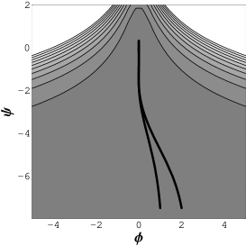
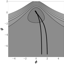
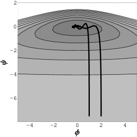
(a)                                         (b)                                         (c)

Figure 1: Typical trajectories, on the contour plot of the potential $U(\psi,\phi)$, for: (a) $\rho=10$, (b) $\rho=1$, (c) $\rho=0.1$, in the case with $\gamma=0$. The initial conditions for $\psi(t)$ and $\phi(t)$ are $(\psi(0),\phi(0))=(-7.6,1)$ and $(\psi(0),\phi(0))=(-7.6,2)$.

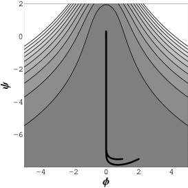
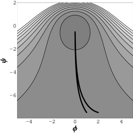
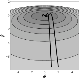
(a)                                         (b)                                         (c)

Figure 2: Typical trajectories, on the contour plot of the potential $U(\psi,\phi)$, for: (a) $\rho=10$, (b) $\rho=1$, (c) $\rho=0.1$, in the case with $\gamma=1$. The initial conditions for $\psi(t)$ and $\phi(t)$ are $(\psi(0),\phi(0))=(-7.6,1)$ and $(\psi(0),\phi(0))=(-7.6,2)$.

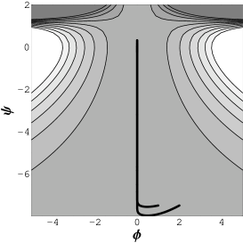
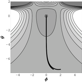
(a)                                         (b)                                         (c)

Figure 3: Typical trajectories, on the contour plot of the potential $U(\psi,\phi)$, for: (a) $\rho=10$, (b) $\rho=1$, (c) $\rho=0.1$, in the case with $\gamma=2$. The initial conditions for $\psi(t)$ and $\phi(t)$ are $(\psi(0),\phi(0))=(-7.6,1)$ and $(\psi(0),\phi(0))=(-7.6,2)$.

Before closing this section, we write down the slow-roll parameter according to Ref. CEOS here. They are, in our present notation,

$$\epsilon = \frac{U_{\psi}^{2}+U_{\phi}^{2}}{U^{2}}\,,$$ (6)

$$\eta_{\sigma\sigma} = \frac{2(\dot{\psi}^{2}U_{\psi\psi}+\dot{\phi}^{2}U_{\phi\phi}+2\dot{\psi}\dot{\phi}U_{\psi\phi})}{(\dot{\psi}^{2}+\dot{\phi}^{2})U}\,,$$ (7)

where $U_{\psi}\equiv\frac{\partial U}{\partial\psi}$, etc. and the dot denotes the time derivative. Further, if we assume that the scalar potential $V(\phi)$ is slow-roll type, the analysis on approximate solutions will be identical to the result of Cruz-Dombriz et al. CEOS , independently to the value of $\gamma$ (thus, we do not repeat it further).

III quantum cosmology of the extended $R^{2}$ model

We now turn to the quantum cosmology of our $K$-essentially modified model. Quantum cosmology of the Starobinsky model has already been discussed by many authors Vilenkin ; HL ; HW ; MMS2 . Here, we shall quantize our model along with the most standard minisuperspace method of ones used by them.

We shall consider the metric of the form

$$ds^{2}=g_{\mu\nu}dx^{\mu}dx^{\nu}=\frac{1}{K}a^{2}(t)(-dt^{2}+d\tilde{\Omega}_{3}^{2})\,,$$ (8)

where $d\tilde{\Omega}^{2}_{3}$ is the line element on a three-dimensional maximally-symmetric manifold, whose Ricci tensor is given by

$$\tilde{R}_{j}^{i}=2k\delta_{j}^{i}\,,$$ (9)

where $i,j=1,2,3$ and $k$ is a constant, which has been normalized to $0$, $\pm 1$. $K$ is a constant which will be used to arrange the cosmological Lagrangian into a canonical form. We also assume that the scalar field $\phi$ is homogeneous on the three dimensional manifold, i.e., $\phi=\phi(t)$.

The scalar curvature of the spacetime is computed with the metric (8) as

$$R=6K\left(\frac{\ddot{a}}{a^{3}}+\frac{k}{a^{2}}\right)\,,$$ (10)

where the dot denotes the derivative with respect to $t$. Thus, the effective cosmological Lagrangian $L$, which expresses the action as $S=\int dt\,L$, can be obtained as

$$L = \frac{2\pi^{2}\alpha}{K}\left[6\left(-\dot{a}^{2}+ka^{2}\right)+\frac{1}{2}a^{2}\dot{\phi}^{2}-\frac{a^{4}}{K}V(\phi)\right]$$ (11)

$$\qquad\qquad\quad+\frac{2\pi^{2}\beta}{2}\left[6\left(\frac{\ddot{a}}{a}+k\right)+\frac{1}{2}\dot{\phi}^{2}-\gamma\frac{a^{2}}{K}V(\phi)\right]^{2}$$

$$= \frac{2\pi^{2}\alpha}{K}\left[6\left(-\dot{a}^{2}+ka^{2}\right)+\frac{1}{2}a^{2}\dot{\phi}^{2}-\frac{a^{4}}{K}V(\phi)\right]+\frac{1}{36\pi^{2}\beta}\bar{Q}^{2}(a,\dot{a},\ddot{a},\phi,\dot{\phi})\,,$$

where we added the standard Gibbons–Hawking–York boundary term York ; GH , and further we defined

$$\bar{Q}\equiv 6\pi^{2}\beta\left[6\left(\frac{\ddot{a}}{a}+k\right)+\frac{1}{2}\dot{\phi}^{2}-\gamma\frac{a^{2}}{K}V(\phi)\right]\,.$$ (12)

We now select a specific value for $K$, as $K=24\pi^{2}\alpha$, for convenience in the present section. We also consider an equivalent Lagrangian $L^{\prime}$ as follows:

$$L^{\prime}(a,\dot{a},Q,\dot{Q},\phi,\dot{\phi}) \equiv L-\frac{1}{36\pi^{2}\beta}(Q-\bar{Q})^{2}-2\frac{d}{dt}\left(\frac{\dot{a}}{a}Q\right)$$ (13)

$$= \frac{1}{12}\left[-6\dot{a}^{2}+\frac{1}{2}a^{2}\dot{\phi}^{2}\right]+\frac{1}{3}\left[6\frac{\dot{a}^{2}}{a^{2}}Q-6\frac{\dot{a}}{a}\dot{Q}+\frac{1}{2}Q\dot{\phi}^{2}\right]-{\cal U}(a,Q,\phi)$$

$$= \left[-\frac{1}{2}\left(a+\frac{4Q}{a}\right)^{\cdot}\dot{a}+\frac{1}{24}(a^{2}+4Q)\dot{\phi}^{2}\right]-{\cal U}(a,Q,\phi)\,,$$

with

$${\cal U}(a,Q,\phi)\equiv-\frac{k}{2}(a^{2}+2Q)+\frac{1}{36\pi^{2}\beta}Q^{2}+\frac{1}{288\pi^{2}\alpha}(a^{4}+4\gamma a^{2}Q)V(\phi)\,.$$ (14)

We have introduced a new variable $Q$, which can be integrated out trivially as a Gaussian integral.

Here, one can use new coordinates $x$ and $y$:

$$x=\frac{2Q}{a}\,,\quad y=a+\frac{2Q}{a}\,.$$ (15)

Additionally, one can define $\varphi\equiv\phi/(2\sqrt{3})$ to simplify the form of the Lagrangian. Then, the following Lagrangian is obtained:

$$L^{\prime}=\frac{1}{2}\left(\dot{x}^{2}-\dot{y}^{2}\right)+\frac{1}{2}(y^{2}-x^{2})\dot{\varphi}^{2}-{\cal U}(x,y,\varphi)\,,$$ (16)

where

$${\cal U}(x,y,\varphi)\equiv-\frac{k}{2}(y^{2}-x^{2})+\frac{1}{144\pi^{2}\beta}x^{2}(y-x)^{2}+\frac{1}{288\pi^{2}\alpha}(y-x)^{3}[y+(2\gamma-1)x]V(2\sqrt{3}\varphi)\,.$$ (17)

Furthermore, using a set of variables $r$ and $\theta$ defined as

$$x=r\sinh\theta\,,\quad y=r\cosh\theta\,,$$ (18)

we obtain the expression

$$L^{\prime}=\frac{1}{2}\left[-\dot{r}^{2}+r^{2}(\dot{\theta}^{2}+\dot{\varphi}^{2})\right]-{\cal U}(r,\theta,\varphi)\,,$$ (19)

with

$${\cal U}(r,\theta,\varphi)=-\frac{kr^{2}}{2}+\frac{r^{4}}{576\pi^{2}\beta}(1-e^{-2\theta})^{2}+\frac{r^{4}}{288\pi^{2}\alpha}\left[\gamma e^{-2\theta}-(\gamma-1)e^{-4\theta}\right]V(2\sqrt{3}\varphi)\,.$$ (20)

Comparing with the expression in the previous section, we find that the correspondences are $\phi=2\sqrt{3}\varphi$ and $\psi=-2\sqrt{3}\theta$.

One can then treat $r$, $\theta$, and $\varphi$ as independent coordinates and define their canonical momenta in the usual way:

$$P_{r}=\frac{\partial L^{\prime}}{\partial\dot{r}}=-\dot{r}\,,\quad P_{\theta}=\frac{\partial L^{\prime}}{\partial\dot{\theta}}=r^{2}\dot{\theta}\,,\quad P_{\varphi}=\frac{\partial L^{\prime}}{\partial\dot{\varphi}}=r^{2}\dot{\varphi}\,.$$ (21)

One can then define the classical Hamiltonian by the normal Legendre transformation:

$$H=P_{r}\dot{r}+P_{\theta}\dot{\theta}+P_{\varphi}\dot{\varphi}-L^{\prime}=\frac{1}{2}\left[-P_{r}^{2}+\frac{1}{r^{2}}\left(P_{\theta}^{2}+P_{\varphi}^{2}\right)\right]+{\cal U}(r,\theta,\varphi)\,.$$ (22)

The quantization scheme requires replacing $P_{r}$, $P_{\theta}$, and $P_{\varphi}$ by $-i\frac{\partial}{\partial r}$, $-i\frac{\partial}{\partial\theta}$, and $-i\frac{\partial}{\partial\varphi}$, respectively. This replacement results in the derivation of the Hamiltonian operator $\hat{H}$. The Wheeler–De Witt (WDW) equation reads $\hat{H}\Psi=0$, i.e.,

$$\left[\frac{1}{r^{s}}\frac{\partial}{\partial r}r^{s}\frac{\partial}{\partial r}-\frac{1}{r^{2}}\left(\frac{\partial^{2}}{\partial\theta^{2}}+\frac{\partial^{2}}{\partial\varphi^{2}}\right)+2{\cal U}(r,\theta,\varphi)\right]\Psi(r,\theta,\varphi)=0\,,$$ (23)

where $\Psi$ is the wave function of the universe. Here, we took the factor ordering ambiguity into consideration through the factor $r^{s}$.

To solve the WDW equation, we have to specify the boundary conditions. In this section, we restrict ourselves on the case of the closed universe, $k=1$. In this case, the curvature-dependent term in ${\cal U}$ makes a finite potential barrier between $r\sim 0$ and $r\gg\sqrt{\beta}$. We first consider the behavior of the wave function in the vicinity of $r=0$. In the beginning of the universe, or the initial state of the universe, $r$ should be very small. For $r\ll\sqrt{\beta}$, we can neglect the terms of order of $r^{4}$, i.e.,

$$\left[\frac{1}{r^{s}}\frac{\partial}{\partial r}r^{s}\frac{\partial}{\partial r}-\frac{1}{r^{2}}\left(\frac{\partial^{2}}{\partial\theta^{2}}+\frac{\partial^{2}}{\partial\varphi^{2}}\right)-r^{2}\right]\Psi(r,\theta,\varphi)=0\,.$$ (24)

For small $r$, both authors of Vilenkin ; MMS2 took $s=0$ and assumed that $\Psi$ is independent of the other variables. If we also assume that the wave function is almost independent of $\theta$ and $\varphi$, the solution of (24) is the same as the solution $\Psi\propto\sqrt{r}K_{1/4}(r^{2}/2)$, where $K_{\nu}(z)$ is the modified Bessel function of the second kind Vilenkin ; MMS2 . We here point out that if $s=1$, the solution of (24) is given by

$$\Psi\propto\int\int A(l,m)\,K_{i\sqrt{l^{2}+m^{2}}/2}(r^{2}/2)e^{il\theta+im\varphi}dldm\,,$$ (25)

where $A(l,m)$ represents for the amplitude of each elementary wave. In both cases, we find

$$\Psi\propto e^{-r^{2}/2}\mbox{~{}~{}for large~{}}r\,.$$ (26)

The problem of the ordering is also discussed in Appendix A.

For the region of $0<r<\sqrt{\beta}$, we use the WKB approximation, i.e., we want to find the solution that has the approximate form $\Psi=Ae^{-B}$. The lowest order equation tells

$$\left(\frac{\partial B}{\partial r}\right)^{2}-\frac{1}{r^{2}}\left[\left(\frac{\partial B}{\partial\theta}\right)^{2}+\left(\frac{\partial B}{\partial\varphi}\right)^{2}\right]+2{\cal U}(r,\theta,\varphi)=0\,.$$ (27)

Note that the factor ordering does not affect the expression because we consider $B$ as a smooth function at relatively large $r$. If the terms proportional to $\left(\frac{\partial B}{\partial\theta}\right)^{2}$ and $\left(\frac{\partial B}{\partial\varphi}\right)^{2}$ can be neglected Vilenkin ; MMS2 , we find

$$\frac{\partial B}{\partial r}=\pm\sqrt{-2{\cal U}(r,\theta,\varphi)}=\pm r\left[1-r^{2}{\cal V}(\theta,\varphi)\right]^{1/2}\,,$$ (28)

where

$${\cal V}(\theta,\varphi)\equiv\frac{1}{144\pi^{2}\alpha}\left[\frac{1}{2\beta^{\prime}}(1-e^{-2\theta})^{2}+\left[\gamma e^{-2\theta}-(\gamma-1)e^{-4\theta}\right]V(2\sqrt{3}\varphi)\right]\,.$$ (29)

Therefore, we obtain $B$ in the WKB approximation as

$$B_{\pm}=\frac{\pm 1}{3{\cal V}(\theta,\varphi)}\left\{1-[1-r^{2}{\cal V}(\theta,\varphi)]^{3/2}\right\}\,.$$ (30)

One can see that $B_{+}\rightarrow r^{2}/2$ for $r\rightarrow 0$. This agrees the asymptotic behavior of the wave function for a small $r$, (26), if we consider the tunneling wave function à la Vilenkin Vilenkin .

The wave function after tunneling, $r\gg\sqrt{\beta}$, can be obtained by analytic continuation, thus we get

$$\Psi_{\pm}\propto\exp\left[\mp\frac{1}{3{\cal V}(\theta,\varphi)}\left\{1+i[1-r^{2}{\cal V}(\theta,\varphi)]^{3/2}\right\}\pm\frac{i\pi}{4}\right]\,.$$ (31)

The ‘tunneling’ wave function à la Vilenkin is proportional to $\Psi_{+}$, while the wave function with the ‘no-boundary’ boundary condition is proportional to $e^{\frac{2}{3{\cal V}}}\Psi_{+}+\Psi_{-}$ MMS2 . Thus, the distribution is given by MMS2

$$|\Psi|^{2}\propto\exp\left[-\frac{2}{3{\cal V}(\theta,\varphi)}\right]\,\quad\mbox{for the `tunneling' boundary condition}\,,$$ (32)

$$|\Psi|^{2}\propto\exp\left[+\frac{2}{3{\cal V}(\theta,\varphi)}\right]\,\quad\mbox{for the `no-boundary' boundary condition}\,.$$ (33)

The no-boundary wave function for a two-field inflation model was studied by Hwang et al. HKY . Their study can be applied to our model with the canonical scalar kinetic terms, provided that the potential ${\cal V}(\theta,\varphi)$ is approximated by $\frac{1}{2}{\cal V}_{\theta\theta}\theta^{2}+\frac{1}{2}{\cal V}_{\varphi\varphi}\varphi^{2}$ (i.e., it is assumed that $V(0)=V^{\prime}(0)=0$). According to Ref. HKY , if ${\cal V}_{\varphi\varphi}\ll{\cal V}_{\theta\theta}$, cosmic inflation can occur with the number of $e$-foldings

$${\cal N}\approx\frac{{\cal V}_{\theta\theta}}{{\cal V}_{\varphi\varphi}}=\frac{\alpha}{\beta V^{\prime\prime}(0)}\,,$$ (34)

by analysis using an approximation ${\cal V}\approx\frac{1}{2}{\cal V}_{\theta\theta}\theta^{2}+{\cal V}_{0}$, where ${\cal V}_{0}=\frac{1}{2}{\cal V}_{\varphi\varphi}\varphi^{2}\approx const$ HKY . Therefore, as an inflationary two-field model, our model can work well.

Here, we confirmed that our model admits no-boundary wave function which can provide an appropriate initial condition for the two-field inflation model in the preceding study of Hwang et al. HKY . Although the quantum effect on evolution of the universe is also an important subject to study, we think that it is beyond our present scope and should be left aside for future work.

Before closing this section, we place a comment on another method of analysis on the wave function of $r\ll\sqrt{\beta}$ (which is not limited on the extended model). If one removes the assumption that $\Psi$ is independent of $\theta$, we can write the WDW equation in terms of $x$ and $y$ from Eqs. (16) and (17):

$$\left[-\frac{\partial^{2}}{\partial x^{2}}+x^{2}+\frac{\partial^{2}}{\partial y^{2}}-y^{2}\right]\Psi(x,y)=0\,,$$ (35)

and the wave packet solution is Kiefer

$$\Psi(x,y)=\sum_{n}A_{n}\frac{H_{n}(x)H_{n}(y)}{2^{n}n!}\exp\left[-\frac{1}{2}(x^{2}+y^{2})\right]\,,$$ (36)

where $A_{n}$ is amplitudes. The asymptotic behavior at $r\rightarrow\infty$ is $\Psi\sim\exp[-\frac{1}{2}r^{2}]$ can be obtained for $\theta\sim 0$ (i.e., $x\sim 0$).

IV modified positive-definite action

Positive-definite action for gravity was conjectured by Horowitz Horowitz about three decades ago. Under some appropriate conditions, this theory can be considered as the high-curvature limit of $R+\beta R^{2}/2$ theory. An extension of the model with a scalar field is defined by the following action:

$$S_{S}=\frac{\beta}{2}\int d^{4}x\,\sqrt{-g}\,\left[R-\frac{1}{2}(\nabla\phi)^{2}-\gamma V(\phi)\right]^{2}\,.$$ (37)

By a similar method to that seen in Sec. II, the equivalent action at classical level is obtained as

$$S=\int d^{4}x\sqrt{-g}\,\left\{\beta\chi\left[R-\frac{1}{2}(\nabla\phi)^{2}-\gamma V(\phi)\right]-\frac{\beta}{2}\chi^{2}\right\}\,.$$ (38)

An appropriate Weyl transformation with the apparent auxiliary field $\chi$ is attained by the transformation $g_{\mu\nu}=\chi^{-1}\tilde{g}_{\mu\nu}$. Then, we obtain

$$S=\int d^{4}x\sqrt{-\tilde{g}}\,\,\beta\left[\tilde{R}-\frac{1}{2}(\tilde{\nabla}\phi)^{2}-\frac{1}{2}(\tilde{\nabla}\psi)^{2}-e^{\frac{1}{\sqrt{3}}\psi}\gamma V(\phi)-\frac{1}{2}\right]\,,$$ (39)

where we defined $\psi\equiv-\sqrt{3}\ln\chi$.

There appears the cosmological constant as the last term in the Lagrangian in (39). In our present model, however, the scalar potential which can be arbitrarily chosen is included in the Lagrangian. Thus, a general two-field model for cosmic acceleration can be constructed in our scheme.

Classical cosmological solutions are known to be obtained analytically in some cases, but we leave the derivation of solutions for the next section, where we exhibit solvable pure $R^{p}$ models.

Quantum cosmology of $R^{2}$ gravity has been investigated in many papers, including Horowitz ; Schmidt1 ; Schmidt2 . We study our extended model by the standard method used by them. As in the previous section, we obtain the effective cosmological Lagrangian of the model:

$$L\equiv\frac{2\pi^{2}\beta}{2}\left[6\left(\frac{\ddot{a}}{a}+1\right)+\frac{1}{2}\dot{\phi}^{2}-\gamma\frac{a^{2}}{K}V(\phi)\right]^{2}=\frac{1}{36\pi^{2}\beta}\bar{Q}^{2}(a,\dot{a},\ddot{a},\phi,\dot{\phi})\,,$$ (40)

where $\bar{Q}$ is defined as in Eq. (12), and other metric definitions are the same as well in the previous section. The equivalent Lagrangian now has the form

$$L^{\prime}(a,\dot{a},Q,\dot{Q},\phi,\dot{\phi}) \equiv L-\frac{1}{36\pi^{2}\beta}(Q-\bar{Q})^{2}-2\frac{d}{dt}\left(\frac{\dot{a}}{a}Q\right)$$ (41)

$$= -2\left(\frac{Q}{a}\right)^{\cdot}\dot{a}+\frac{1}{6}Q\dot{\phi}^{2}-{\cal U}(a,Q,\phi)\,,$$

where

$${\cal U}(a,Q,\phi)\equiv\frac{1}{36\pi^{2}\beta}Q^{2}-2kQ+\frac{a^{2}}{3K}Q\gamma V(\phi)\,.$$ (42)

Here, one can use new coordinates $x$ and $y$:

$$x=\frac{Q}{a}-a\,,\quad y=a+\frac{Q}{a}\,.$$ (43)

We define $\varphi\equiv\phi/(2\sqrt{3})$ to simplify the form of the Lagrangian. Then, one can obtain

$$L^{\prime}=\frac{1}{2}\left(\dot{x}^{2}-\dot{y}^{2}\right)+\frac{1}{2}(y^{2}-x^{2})\dot{\varphi}^{2}-{\cal U}(x,y,\phi)\,,$$ (44)

where

$${\cal U}(x,y,\phi)\equiv-\frac{k}{2}(y^{2}-x^{2})+\frac{1}{576\pi^{2}\beta}(y^{2}-x^{2})^{2}+\frac{1}{48K}(y-x)^{2}(y^{2}-x^{2})\gamma V(2\sqrt{3}\varphi)\,.$$ (45)

Using a set of variables $r$ and $\theta$ defined as $x=r\sinh\theta$ and $y=r\cosh\theta$, we obtain the expression

$$L^{\prime}=\frac{1}{2}\left[-\dot{r}^{2}+r^{2}(\dot{\theta}^{2}+\dot{\varphi}^{2})\right]-{\cal U}(r,\theta,\varphi)\,,$$ (46)

with

$${\cal U}(r,\theta,\varphi)=-\frac{k}{2}r^{2}+\frac{r^{4}}{576\pi^{2}\beta}+\frac{1}{48K}r^{4}e^{-2\theta}\gamma V(2\sqrt{3}\varphi)\,.$$ (47)

Then, we obtain the Hamiltonian

$$H = \frac{1}{2}\left[-P_{r}^{2}+\frac{1}{r^{2}}\left(P_{\theta}^{2}+P_{\varphi}^{2}\right)\right]+{\cal U}(r,\theta,\varphi)\,.$$ (48)

and the WDW equation

$$\left[\frac{1}{r}\frac{\partial}{\partial r}r\frac{\partial}{\partial r}-\frac{1}{r^{2}}\left(\frac{\partial^{2}}{\partial\theta^{2}}+\frac{\partial^{2}}{\partial\varphi^{2}}\right)+2{\cal U}(r,\theta,\varphi)\right]\Psi(r,\theta,\varphi)=0\,,$$ (49)

as in the previous section (and we fixed here the ordering by $s=1$).

Let us consider the solution of the WDW equation. The case of a closed universe is similarly analyzable as the model in the previous section. Therefore, we here consider the case of a flat universe, $k=0$.

Moreover, if $V(\phi)\equiv 0$ or $V(\phi)$ is negligible, the equation becomes

$$\left[\frac{1}{r}\frac{\partial}{\partial r}r\frac{\partial}{\partial r}-\frac{1}{r^{2}}\left(\frac{\partial^{2}}{\partial\theta^{2}}+\frac{\partial^{2}}{\partial\varphi^{2}}\right)+\frac{r^{4}}{288\pi^{2}\beta}\right]\Psi(r,\theta,\varphi)=0\,.$$ (50)

The solution of this equation can be expressed by the form of superposition:

$$\Psi = \int\int\left[A(l,m)J_{i\frac{\sqrt{l^{2}+m^{2}}}{3}}(r^{3}/(36\sqrt{2\beta}\pi))\right.$$ (51)

$$\qquad\quad\left.+B(l,m)J_{-i\frac{\sqrt{l^{2}+m^{2}}}{3}}(r^{3}/(36\sqrt{2\beta}\pi))\right]e^{il\theta+im\varphi}dldm\,,$$

where $J_{\nu}(z)$ is the Bessel function and $A(l,m)$ and $B(l,m)$ are amplitudes for each elementary wave. Because of the absence of potential wall due to the curvature and the scalar potential, the behavior of the wave function is generally oscillatory in the direction of $r$. Since there is no tunneling, we assume an appropriate wave packet form in the beginning of the universe Kiefer ; KNw ; Kiefer1 to study further.

As seen here, it is known that some limited cases can be solved exactly. In the next section, we pursue the solvable model of $K$-essentially modified pure $R^{p}$ gravity, where $p$ is a rational number.

V soluble models for $K$-essentially modified pure $R^{p}$ gravity

In this section, we consider an extension of pure $R^{p}$ gravity in $D$ dimensional spacetime. We start with the action

$$S=\frac{\beta}{p(p-1)}\int d^{D}x\,\sqrt{-g}\,\left[R-\frac{1}{2}(\nabla\phi)^{2}-\gamma V(\phi)\right]^{p}\,.$$ (52)

As in the previous sections, we can use an auxiliary field $\chi$ to obtain classically equivalent action:

$$S=\beta\int d^{D}x\sqrt{-g}\,\left\{\frac{\chi^{p-1}}{p-1}\left[R-\frac{1}{2}(\nabla\phi)^{2}-\gamma V(\phi)\right]-\frac{\chi^{p}}{p}\right\}\,.$$ (53)

We eliminate the $\chi$-dependence in front of $R$ in the action (53) by a Weyl transformation. We consider a metric $\tilde{g}_{\mu\nu}$ which satisfies $\sqrt{-g}\chi^{p-1}R=\sqrt{-\tilde{g}}\tilde{R}+\cdots$, where $\tilde{R}$ is the Ricci scalar constructed from $\tilde{g}_{\mu\nu}$. Now, we select $g_{\mu\nu}=\chi^{-\frac{2(p-1)}{D-2}}\tilde{g}_{\mu\nu}$ in this time. Then, we obtain

$$S = \frac{\beta}{p-1}\int d^{D}x\sqrt{-\tilde{g}}\left[\tilde{R}-\frac{1}{2}(\tilde{\nabla}\phi)^{2}-\frac{1}{2}(\tilde{\nabla}\psi)^{2}\right.$$ (54)

$$\qquad\qquad\qquad\qquad\left.-e^{\sqrt{\frac{2}{(D-1)(D-2)}}\psi}\gamma V(\phi)-\frac{p-1}{p}e^{\sqrt{\frac{2}{(D-1)(D-2)}}\frac{p-D/2}{p-1}\psi}\right]\,.$$

Here, we defined $\psi\equiv-\sqrt{\frac{2(D-1)}{D-2}}(p-1)\ln\chi$. Note that the scalar field $\phi$ has a canonical kinetic term again in the model.

We expect that the exact solutions of simple models are useful to reveal some subtle features of the cosmological dynamical system MP ; PM ; TW ; Ohta2 ; LMPX ; Kaloper ; CGG ; Roy ; ANL ; ALNW ; KKST . Here, we investigate the cases with specific parameters, where the exact classical and quantum cosmological solutions can be obtained.

For this purpose, we restrict ourselves on a flat $D$-dimensional spacetime and choose the metric as

$$d\tilde{s}^{2}=-e^{2n(t)}dt^{2}+e^{2\tilde{a}(t)}\sum_{i=1}^{D-1}(dx^{i})^{2}\,.$$ (55)

From this metric, the scalar curvature can be calculated as

$$\tilde{R}=e^{-2n}[2(D-1)(\ddot{\tilde{a}}-\dot{n}\dot{\tilde{a}})+D(D-1)\dot{\tilde{a}}^{2}]\,.$$ (56)

Fixing a gauge $n(t)=(D-1)\tilde{a}(t)$, one can find that the cosmological Lagrangian can be rewritten as

$$L= -(D-1)(D-2)\dot{\tilde{a}}^{2}+\frac{1}{2}\dot{\phi}^{2}+\frac{1}{2}\dot{\psi}^{2}$$ (57)

$$-e^{2(D-1)\tilde{a}+\sqrt{\frac{2}{(D-1)(D-2)}}\psi}\gamma V(\phi)-\frac{p-1}{p}e^{2(D-1)\tilde{a}+\sqrt{\frac{2}{(D-1)(D-2)}}\frac{p-D/2}{p-1}\psi}\,,$$

apart from an overall normalization which differs from the previous one.

We find that exact solutions can be obtained for the system governed by the Lagrangian (57) in the following two cases: A. $p=D/2$ and $\gamma V(\phi)=0$, B. $p=1-1/(2D)$ and $\gamma V(\phi)=\frac{1}{2}f^{2}\exp[\sqrt{\frac{2D}{D-1}}g\phi]$. The case of $p=2$ and $D=4$ seen in the previous section belongs to the case A. We will exhibit classical and quantum exact solutions in both cases A and B.

Note that the equivalence of the higher order theory and the reduced theory by using an auxiliary field is classically valid, while the equivalence of them in quantum physics is not always clear. As seen in previous sections, quantum $R^{2}$ gravity can be rewritten by adding quadratic term including a new variable. This redefinition is equivalent to adding a Gaussian integration in view of path integral. For a general power $p$, similar addition of a new variable may cause a problem of measure in path integral. Nevertheless, we consider the quantization of the system with an ‘auxiliary’ field as an ‘effective’ theory, which can grasp some feature and tendency of behavior of dynamical variables in the physical system.

Now, we show the solutions in solvable cases.

V.1 $p=D/2$ and $\gamma V(\phi)=0$

The first case is a natural generalization of pure $R^{2}$ gravity in four dimensions. In this case, $V(\phi)\equiv 0$ is assumed and $p=D/2$ is chosen. The cosmological Lagrangian includes two massless scalar field, aside from the cosmological term, in this case. Then, the Lagrangian (57) becomes

$$L=-(D-1)(D-2)\dot{\tilde{a}}^{2}+\frac{1}{2}\dot{\phi}^{2}+\frac{1}{2}\dot{\psi}^{2}-\frac{D-2}{D}e^{2(D-1)\tilde{a}}\,.$$ (58)

In order to make it simpler, we introduce normalization and other constants as

$$X\equiv\sqrt{2(D-1)(D-2)}\tilde{a}\,,\quad\lambda\equiv\sqrt{\frac{D-1}{2(D-2)}}\,,\quad\delta\equiv\sqrt{\frac{2(D-2)}{D}}\,.$$ (59)

We now obtain the simplified Lagrangian

$$L=-\frac{1}{2}\dot{X}^{2}-\frac{\delta^{2}}{2}e^{2\lambda X}+\frac{1}{2}\dot{\phi}^{2}+\frac{1}{2}\dot{\psi}^{2}\,,$$ (60)

and the Hamiltonian derived from the Lagrangian

$$H=H_{X}+H_{\phi}+H_{\psi}\,.$$ (61)

Here, the separated Hamiltonians are

$$H_{X}=-\frac{1}{2}p_{X}^{2}+\frac{\delta^{2}}{2}e^{2\lambda X}\,,\quad H_{\phi}=\frac{1}{2}p_{\phi}^{2}\,,\quad H_{\psi}=\frac{1}{2}p_{\psi}^{2}\,,$$ (62)

where $p_{X}=-\dot{X}$, $p_{\phi}=\dot{\phi}$, and $p_{\psi}=\dot{\psi}$.

From the Lagrangian (60), we find that the variables are separated and $X$ obeys the Liouville equation in one dimension. Therefore, the separated Hamiltonians $H_{X}$, $H_{\phi}$, and $H_{\psi}$ become constants $E_{X}$, $E_{\phi}$, and $E_{\psi}$, respectively, if the individual solutions are substituted. Thus, the solutions can be written down as

$$X(t) = \frac{1}{2\lambda}\ln\frac{q_{X}^{2}}{\sinh^{2}q_{X}\delta\lambda(t-t_{X})}\,,\qquad E_{X}=-\frac{q_{X}^{2}\delta^{2}}{2}\,,$$ (63)

$$\phi(t) = q_{\phi}(t-t_{\phi})\,,\quad E_{\phi}=\frac{q_{\phi}^{2}}{2}\,,$$ (64)

$$\psi(t) = q_{\psi}(t-t_{\psi})\,,\quad E_{\psi}=\frac{q_{\psi}^{2}}{2}\,,$$ (65)

where $q_{X}$, $q_{\phi}$, $q_{\psi}$, $t_{X}$, $t_{\phi}$, and $t_{\psi}$ are integration constants. Remembering that we treat the general relativistic system, the constants should satisfy the relation

$$E_{X}+E_{\phi}+E_{\psi}=0\,.$$ (66)

Therefore, we can finally write the solution as

$$e^{2(D-1)\tilde{a}(t)}=e^{2\lambda X}=\frac{q_{\phi}^{2}+q_{\psi}^{2}}{\delta^{2}\sinh^{2}\sqrt{q_{\phi}^{2}+q_{\psi}^{2}}\lambda(t-t_{X})}\,,$$

$$\phi(t)=q_{\phi}(t-t_{\phi})\,,\quad\psi(t)=q_{\psi}(t-t_{\psi})\,.$$ (67)

One can check the solution through a special case, $q_{\phi}=q_{\psi}\rightarrow 0$. In this limit, one finds $e^{(D-1)\tilde{a}(t)}=\delta^{-1}\lambda^{-1}|t_{X}-t|^{-1}$. If one uses the ‘canonical’ cosmic time $\tau$, $d\tau\equiv e^{n}dt=e^{(D-1)\tilde{a}(t)}dt$, one obtains $\tau=-\delta^{-1}\lambda^{-1}\ln|t_{X}-t|$. Accordingly, $e^{(D-1)\tilde{a}(t)}\propto e^{\delta\lambda\tau}$ can be found. This exponential expansion is caused by the cosmological constant, since the scalar fields are frozen in this limit. For general $q_{\phi}$ and $q_{\psi}$, the asymptotic behavior of the scale factor $e^{\tilde{a}}$ can be found as: $e^{\tilde{a}}\sim e^{\delta\lambda\tau/(D-1)}$ for $\tau\rightarrow\infty$ and $e^{\tilde{a}}\sim\tau^{1/(D-1)}$ for $\tau\sim 0$.

We now turn to the study of quantum cosmology in this case. The WDW equation becomes

$$\left[\frac{\partial^{2}}{\partial X^{2}}+\delta^{2}\,e^{2\lambda X}-\frac{\partial^{2}}{\partial\phi^{2}}-\frac{\partial^{2}}{\partial\psi^{2}}\right]\Psi(X,\phi,\psi)=0\,.$$ (68)

The general solution of this wave equation is

$$\Psi(X,\phi,\psi) = \int\int\left[A(l,m)J_{i\sqrt{l^{2}+m^{2}}/\lambda}(\delta e^{\lambda X}/\lambda)\right.$$ (69)

$$\qquad\quad+\left.B(l,m)J_{-i\sqrt{l^{2}+m^{2}}/\lambda}(\delta e^{\lambda X}/\lambda)\right]e^{il\psi+im\phi}dldm\,.$$

Note that $e^{\lambda X}=e^{(D-1)\tilde{a}}$. The expression of (69) seems a different from the solution (51) in four dimensions, because of the choice of time coordinate as well as because of the different set of variables and their normalizations. Nevertheless, the reason of appearance of the similar type of function can be understood easily as follows. In the present section, we obtain $\dot{\psi}=const.$ as a consequence of the gauge choice ($n=(D-1)\tilde{a}$). Thus, we can regard $\psi$ as a ‘time’ in the space of variables in this gauge. Taking the ‘time’ axis simply so as to cross the ‘origin’ where $\psi\approx\theta\approx 0$, the argument $e^{3\tilde{a}}$ appears in the Bessel function in (69), since $e^{3\tilde{a}}=a^{3}=(r/2)^{3}e^{-3\theta}\approx(r/2)^{3}$.

V.2 $p=1-\frac{1}{2D}$ and $\gamma V(\phi)=\frac{1}{2}f^{2}\exp(\sqrt{\frac{2D}{D-1}}g\phi)$

The second case enjoys dynamics of two scalar modes in general. When we set $p=1-\frac{1}{2D}$ and assume $\gamma V(\phi)=\frac{1}{2}f^{2}\exp(\sqrt{\frac{2D}{D-1}}g\phi)$, we obtain the following Lagrangian

$$L= -(D-1)(D-2)\dot{\tilde{a}}^{2}+\frac{1}{2}\dot{\phi}^{2}+\frac{1}{2}\dot{\psi}^{2}$$ (70)

$$-\frac{1}{2}f^{2}e^{\sqrt{\frac{2D}{D-1}}g\phi+2(D-1)\tilde{a}+\sqrt{\frac{2}{(D-1)(D-2)}}\psi}+\frac{1}{2D-1}e^{2(D-1)\tilde{a}+(D-1)\sqrt{\frac{2(D-1)}{D-2}}\psi}\,.$$

We consider a new set of variables:

$$x \equiv \frac{1}{\sqrt{1-g^{2}}}\left[\sqrt{\frac{D-1}{2D}}\left(2(D-1)\tilde{a}+\sqrt{\frac{2}{(D-1)(D-2)}}\psi\right)+g\phi\right]\,,$$ (71)

$$y \equiv \frac{1}{\sqrt{1-g^{2}}}\left[\phi+g\sqrt{\frac{D-1}{2D}}\left(2(D-1)\tilde{a}+\sqrt{\frac{2}{(D-1)(D-2)}}\psi\right)\right]\,,$$ (72)

$$z \equiv \sqrt{\frac{D-1}{2D}}\left(2\tilde{a}+(D-1)\sqrt{\frac{2}{(D-1)(D-2)}}\psi\right)\,,$$ (73)

and define constants:

$$\lambda_{1}\equiv\sqrt{\frac{D}{2(D-1)}}\sqrt{1-g^{2}}\,,\quad\lambda_{3}\equiv\sqrt{\frac{D(D-1)}{2}}\,.$$ (74)

Then, we can obtain the simple form of the Lagrangian (70) as

$$L(x,y,z;\dot{x},\dot{y},\dot{z})=-\frac{1}{2}\dot{x}^{2}+\frac{1}{2}\dot{y}^{2}+\frac{1}{2}\dot{z}^{2}-\frac{1}{2}f^{2}e^{2\lambda_{1}x}+\frac{1}{2D-1}e^{2\lambda_{3}z}\,.$$ (75)

Then, the Hamiltonian becomes

$$H=H_{1}+H_{2}+H_{3}\,,$$ (76)

where

$$H_{1}=-\frac{1}{2}p_{x}^{2}+\frac{f^{2}}{2}e^{2\lambda_{1}x}\,,\quad H_{2}=\frac{1}{2}p_{y}^{2}\,,\quad H_{3}=\frac{1}{2}p_{z}^{2}-\frac{1}{2D-1}e^{2\lambda_{2}z},$$ (77)

with $p_{x}=-\dot{x}$, $p_{y}=\dot{y}$, and $p_{z}=\dot{z}$.

Because of separation of variables, each variable can be solved by a solution of the one-dimensional Liouville equation. The values of $H_{i}$ $(i=1,2,3)$ become constants $E_{i}$, if the solutions are substituted into them. The exact solutions are

$$x(t) = \frac{1}{2\lambda_{1}}\ln\frac{q_{1}^{2}}{\sinh^{2}q_{1}f\lambda_{1}(t-t_{1})}\,,\qquad E_{1}=-\frac{q_{1}^{2}f^{2}}{2}\qquad(f>0)$$ (78)

$$x(t) = \frac{1}{2\lambda_{1}}\ln\frac{q_{1}^{2}}{\sin^{2}q_{1}f\lambda_{1}(t-t_{1})}\,,\qquad E_{1}=\frac{q_{1}^{2}f^{2}}{2}\qquad(f>0)$$ (79)

$$x(t) = q_{1}(t-t_{1})\,,\quad E_{1}=-\frac{q_{1}^{2}}{2}\qquad(f=0)$$ (80)

$$y(t)=q_{2}(t-t_{2})\,,\quad E_{2}=\frac{q_{2}^{2}}{2}$$ (81)

$$z(t) = \frac{1}{2\lambda_{3}}\ln\frac{q_{3}^{2}}{\sinh^{2}q_{3}\sqrt{(D-1/2)^{-1}}\lambda_{3}(t-t_{3})}\,,\qquad E_{3}=\frac{q_{3}^{2}}{2D-1}$$ (82)

$$z(t) = \frac{1}{2\lambda_{3}}\ln\frac{q_{3}^{2}}{\sin^{2}q_{3}\sqrt{(D-1/2)^{-1}}\lambda_{3}(t-t_{3})}\,,\qquad E_{3}=-\frac{q_{3}^{2}}{2D-1}$$ (83)

where constants $E_{1}$, $E_{2}$, and $E_{3}$ should satisfy

$$E_{1}+E_{2}+E_{3}=0\,.$$ (84)

Because $E_{2}\geq 0$, possible combinations are ($E_{1}\leq 0,E_{3}\geq 0$), ($E_{1}\geq 0,E_{3}\leq 0$), and ($E_{1}\leq 0,E_{3}\leq 0$).

Power-law inflation LM can be obtain in the case ($E_{1}\leq 0,E_{3}\geq 0$). We find, in this case,

$$e^{(D-1)\tilde{a}}\propto\exp\left(\frac{(D-1)^{3/2}g}{(D-2)\sqrt{2D(1-g^{2})}}qt\right)\frac{[\sinh q\sinh\theta\lambda_{3}(t_{3}-t)]^{\frac{1}{D(D-2)}}}{[\sinh q\cosh\theta\lambda_{1}(t_{1}-t)]^{\frac{(D-1)^{2}}{D(D-2)(1-g^{2})}}}\,.$$ (85)

Assuming $t_{1}<t_{3}$, the scale factor $e^{\tilde{a}}$ increases monotonically in $-\infty<t<t_{1}$. In terms of the cosmic time $\tau$ ($d\tau=\pm e^{(D-1)\tilde{a}}dt$), the scale factor has behavior $e^{\tilde{a}}\sim\tau^{1/(D-1)}$ for $\tau\sim 0$, while $e^{\tilde{a}}\sim\tau^{(D-1)^{2}/(1+D(D-2)g^{2})}$ for $\tau\rightarrow\infty$. Because $(D-1)^{2}/(1+D(D-2)g^{2})>1$, we find that the solution describes power-law inflation. Unfortunately, non-zero coupling $g$ decreases the power. Note that the case with $g=0$ and $\phi\equiv 0$ reduces the model into the one of pure $R^{p}$ gravity, and the effective potential for $\psi$ is very similar to that studied by Mignemi and Pintus MP ; PM .

Now, we turn to quantum cosmology in the present case. The WDW equation is obtained by $\hat{H}\Psi=0$, where $\hat{H}$ is the Hamiltonian (76) in which momenta are replaced by differential operators. Owing to the separation of variables, the general solution for the WDW equation can be obtained easily as

$$\Psi(x,y,z)=\int\int[A(q,\Theta)J_{iq\cosh\Theta/\lambda_{1}}(e^{\lambda_{1}x}/\lambda_{1})+B(q,\Theta)J_{-iq\cosh\Theta/\lambda_{1}}(e^{\lambda_{1}x}/\lambda_{1})]$$

$$\times[C(q,\Theta)J_{iq\sinh\Theta/\lambda_{3}}(e^{\lambda_{3}z}/(\sqrt{D-1/2}\lambda_{3}))+D(q,\Theta)J_{-iq\sinh\Theta/\lambda_{3}}(e^{\lambda_{3}z}/(\sqrt{D-1/2}\lambda_{3}))]$$

$$\times e^{iqy}dqd\Theta\,,$$ (86)

where $A$, $B$, $C$, and $D$ are amplitudes. This form of solution corresponds to the case ($E_{1}<0,E_{3}>0$). Each wave mode is oscillatory, because there is no potential ‘wall’ at all.

VI Summary and discussion

We have shown that a modification of higher order terms in $R$ can bring about interesting cosmological models. The $K$-essential modification, which utilizes a kinetic-term-like combination of a scalar field, realizes a simple addition of a canonical scalar field into the theory. In this paper, we have studied various classical and quantum cosmologies derived from the actions which contain a $K$-essentially modified term of scalar curvature squared or specific powered. Even though the Starobinsky model can explain the recent observations very well, to introduce modifications in the model is a good way to study its robustness and special properties.

An interesting outcome in the present work is finding that there is a class of solvable models in higher order theory with an additional scalar mode. This is due to the fact that the scalar fields have canonical kinetic terms. This simplicity can be a strong motivation to study the solutions for compact objects with strong gravity, such as black holes, in our models and their extensions.

As subjects for future research, we can also consider the following generalization: the $K$-essential modification of supergravity extensions FKR ; FKP1 ; FKP2 of higher order theory, higher dimensional models with and without dimensional reduction KN ; PPW , higher derivative correction CNMOO ; CSSS ; CMP , higher order theories with other than scalar curvature (e.g. ost ).

Appendix A Solvable pure $R^{2}$ gravity in different variables and the factor ordering

A different factor ordering gives a different solution of the WDW equation, at least in a certain region of variables. In this Appendix A, we review the solvable model of pure $R^{2}$ gravity in four dimensions as an example, and considered the factor ordering when the different variables are used.

For the flat four-dimensional spacetime, the pure $R^{2}$ gravity, i.e., in absence of the additional scalar field, is known to be solvable in the minisuperspace formalism Schmidt1 ; Schmidt2 . In such a case, the effective Lagrangian becomes

$$L^{\prime}(a,\dot{a},Q,\dot{Q})=-2\left(\frac{Q}{a}\right)^{\cdot}\dot{a}-\frac{1}{36\pi^{2}\beta}Q^{2}\,,$$ (87)

since the term which comes from the spatial curvature is also absent. If we use new variables $\sigma\equiv a^{3}$ and $\tau\equiv Q/a$, the Lagrangian can be written as

$$L^{\prime}(\sigma,\dot{\sigma},\tau,\dot{\tau})=-\frac{2}{3\sigma^{2/3}}\dot{\sigma}\dot{\tau}-\frac{\sigma^{2/3}\tau^{2}}{36\pi^{2}\beta}\,,$$ (88)

and the Hamiltonian is given by

$$H(\sigma,\tau,P_{\sigma},P_{\tau})=-\frac{3\sigma^{2/3}}{2}\left(P_{\sigma}P_{\tau}-\frac{\tau^{2}}{54\pi^{2}\beta}\right)\,.$$ (89)

Therefore, the WDW equation reads

$$\left(\frac{\partial}{\partial\sigma}\frac{\partial}{\partial\tau}+\frac{\tau^{2}}{54\pi^{2}\beta}\right)\Psi(\sigma,\tau)=0\,.$$ (90)

This equation can be exactly in the form

$$\Psi(\sigma,\tau)=\int_{-\infty}^{\infty}A(\lambda)\exp\left[-\lambda\sigma+\frac{\tau^{3}}{162\pi^{2}\beta\lambda}\right]d\lambda\,,$$ (91)

where $A(\lambda)$ indicates the amplitude Schmidt1 ; Schmidt2 .

Here, we consider the Fourier transform of the elementary wave solution. That is

$$w=\int_{-\infty}^{\infty}\exp\left[-\lambda\sigma+\frac{\tau^{3}}{162\pi^{2}\beta\lambda}\right]e^{-il\theta}d\theta\,.$$ (92)

The definitions of the variables are the same as in the previous sections, i.e.,

$$x=\frac{Q}{a}-a=r\sinh\theta\,,\quad y=a+\frac{Q}{a}=r\cosh\theta\,.$$ (93)

Thus, we find

$$\sigma=a^{3}=\frac{r^{3}}{8}e^{-3\theta}\,,\quad\tau=\frac{Q}{a}=\frac{r}{2}e^{\theta}\,.$$ (94)

Then, we obtain

$$w = \int_{-\infty}^{\infty}\exp\left[-\lambda\frac{r^{3}}{8}e^{-3\theta}+\frac{r^{3}e^{3\theta}}{8\cdot 162\pi^{2}\beta\lambda}-il\theta\right]d\theta$$ (95)

$$= \frac{1}{3}(-i9\sqrt{2\beta}\pi\lambda)^{-il/3}\int_{-\infty}^{\infty}\exp\left[-i\frac{l}{3}t-i\frac{r^{3}}{36\sqrt{2\beta}\pi}\cosh t\right]dt$$

$$\propto K_{il/3}(ir^{3}/(36\sqrt{2\beta}\pi))\,.$$

Because $K_{il/3}(ir^{3}/(36\sqrt{2\beta}\pi))$ is expressed by a linear combination of $J_{\pm il/3}(r^{3}/(36\sqrt{2\beta}\pi))$, general solution can be written by

$$\Psi = \int\int\left[A(l,m)J_{i\frac{l}{3}}(r^{3}/(36\sqrt{2\beta}\pi))\right.$$ (96)

$$\qquad\quad\left.+B(l,m)J_{-i\frac{l}{3}}(r^{3}/(36\sqrt{2\beta}\pi))\right]e^{il\theta}dl\,.$$

This is the form of the general explicit solution of the following equation:

$$\left[\frac{1}{r}\frac{\partial}{\partial r}r\frac{\partial}{\partial r}-\frac{1}{r^{2}}\frac{\partial^{2}}{\partial\theta^{2}}+\frac{r^{4}}{288\pi^{2}\beta}\right]\Psi(r,\theta)=0\,.$$ (97)

We conclude that the exact solution obtained by Schmidt Schmidt1 ; Schmidt2 is equivalent of the solution of (97), where the parameter of ordering $s$ equals to one, whereas the authors of Vilenkin ; MMS2 chose the different factor ordering ($s=0$) in the ‘kinetic’ term (in the Starobinsky model).

References

• (1) A. D. Linde, “Particle physics and inflationary cosmology”, Contemporary Concepts in Physics 5, (Harwood Academic Pub., Philadelphia, 1990).
• (2) J. Ellis and D. Wands, “22. Inflation”, in Review of particle physics, M. Tanabashi et al. (Particle Data Group), Phys. Rev. D98 (2018) 030001, pp. 364–376.
• (3) L. Amendra and S. Tsujikawa, “Dark energy: theory and observations”, (Cambridge University Press, New York, 2010).
• (4) E. J. Copeland, M. Sami and S. Tsujikawa, Int. J. Mod. Phys. D15 (2006) 1753.
• (5) D. H. Weinberg and M. White, “27. Dark Energy”, in Review of particle physics, M. Tanabashi et al. (Particle Data Group), Phys. Rev. D98 (2018) 030001, pp. 406–413.
• (6) S. Nojiri and S. D. Odintsov, Int. J. Geom. Methods Mod. Phys. 04 (2007) 115.
• (7) T. P. Sotiriou and V. Faraoni, Rev. Mod. Phys. 82 (2010) 451.
• (8) S. Capozziello, M. De Laurentis and V. Faraoni, Open Astron. J. 3 (2010) 49.
• (9) A. De Felice and S. Tsujikawa, Living Rev. Rel. 13 (2010) 3.
• (10) S. Nojiri and S. D. Odintsov, Phys. Rep. 505 (2011) 59.
• (11) S. Capozziello and M. De Laurentis, Phys. Rep. 509 (2011) 167.
• (12) T. Clifton, P. G. Ferreir, A. Padilla and C. Skordis, Phys. Rep. 515 (2012) 1.
• (13) K. Koyama, Rept. Prog. Phys. 79 (2016) 046902.
• (14) S. Nojiri, S. D. Odintsov and V. K. Oikonomou, Phys. Rep. 692 (2017) 1.
• (15) M. Ishak, Living Rev. Rel. 22 (2019) 1.
• (16) A. A. Starobinsky, Phys. Lett. B91 (1980) 99.
• (17) A. Vilenkin, Phys. Rev. D32 (1985) 2511.
• (18) M. B. Mijić, M. S. Morris and W.-M. Suen, Phys. Rev. D34 (1986) 2934.
• (19) C. van de Bruck and L. E. Paduraru, Phys. Rev. D92 (2015) 083513.
• (20) C. van de Bruck, P. Dunsby and L. E. Paduraru, Int. J. Mod. Phys. D26 (2017) 1750152.
• (21) T. Mori, K. Kohri and J. White, JCAP 1710 (2017) 044.
• (22) S. Kaneda and S. V. Ketov, Eur. Phys. J. C76 (2016) 26.
• (23) V. H. Cárdenas, S. del Campo and R. Herrera, Mod. Phys. Lett. A18 (2003) 2039.
• (24) S. Myrzakul, R. Myrzakulov and L. Sebastiani, Eur. Phys. J. C75 (2015) 111.
• (25) M. Sharif and I. Nawazish, Astrophys. Space Sci. 361 (2016) 19.
• (26) D. Gorbunov and A. Tokareva, Phys. Lett. B739 (2014) 50.
• (27) K. Bamba, S. D. Odintsov and P. V. Tretyakov, Eur. Phys. J. C75 (2015) 344.
• (28) A. Salvio and A. Mazumdar, Phys. Lett. B750 (2015) 194.
• (29) Y.-C. Wang and T. Wang, Phys. Rev. D96 (2017) 123506.
• (30) Y. Ema, Phys. Lett. B770 (2017) 403.
• (31) A. Salvio, Phys. Lett. B780 (2018) 111.
• (32) M. He, A. A. Starobinsky and J. Yokoyama, JCAP 1805 (2018) 064.
• (33) D. Gorbunov and A. Tokareva, Phys. Lett. B788 (2019) 37.
• (34) A. Gundhi and C. F. Steinwachs, arXiv:1810.10546 [hep-th].
• (35) Á. Cruz-Dombriz, E. Elizalde, S. D. Odintsov and D. Sáez-Gómez, JCAP 1605 (2016) 060.
• (36) C. Armendariz-Picon, V. Mukhanov and P. J. Steinhardt, Phys. Rev. Lett. 85 (2000) 4438.
• (37) J. García-Bellido and D. Wands, Phys. Rev. D53 (1996) 5437.
• (38) A. A. Starobinsky, S. Tsujikawa and J. Yokoyama, Nucl. Phys. B610 (2001) 383.
• (39) D. Wands, N. Bartolo, S. Matarrese and A. Riotto, Phys. Rev. D66 (2002) 043520.
• (40) F. Di Marco and F. Finelli, Phys. Rev. D71 (2005) 123502.
• (41) Z. Lalak, D. Langlois, S. Pokorsky and K. Turzyński, JCAP 0707 (2007) 014.
• (42) T. Wang, Phys. Rev. D82 (2010) 123515.
• (43) C. van de Bruck and M. Robinson, JCAP 1408 (2014) 024.
• (44) Y.-C. Wang and T. Wang, Int. J. Mod. Phys. D27 (2018) 1850026.
• (45) S. W. Hawking and J. C. Luttrell, Nucl. Phys. B247 (1984) 250.
• (46) S. W. Hawking and Z. C. Wu, Phys. Lett. B151 (1985) 15.
• (47) M. B. Mijić, M. S. Morris and W.-M. Suen, Phys. Rev. D39 (1989) 1496.
• (48) J. W. York, Phys. Rev. Lett. 28 (1972) 1082.
• (49) G. W. Gibbons and S. W. Hawking, Phys. Rev. D15 (1977) 2752.
• (50) D.-I. Hwang, S. A. Kim and D.-H. Yeom, Class. Quant. Grav. 32 (2015) 115006.
• (51) C. Kiefer, Nucl. Phys. B341 (1990) 273.
• (52) G. T. Horowitz, Phys. Rev. D31 (1985) 1169.
• (53) H.-J. Schmidt, Phys. Rev. D49 (1994) 6354;
• (54) H.-J. Schmidt, Phys. Rev. D54 (1996) 7906(E).
• (55) Y. Kazama and R. Nakayama, Phys. Rev. D32 (1985) 2500.
• (56) C. Kiefer, Phys. Rev. D38 (1988) 1761.
• (57) S. Mignemi and N. Pintus, Gen. Rel. Grav. 47 (2015) 51.
• (58) N. Pintus and S. Mignemi, Journal of Physics: Conf. Series 956 (2018) 012022.
• (59) P. K. Townsend and M. N. R. Wohlfarth, Phys. Rev. Lett. 91 (2003) 061302.
• (60) N. Ohta, Phys. Rev. Lett. 91 (2003) 061303.
• (61) H. Lü, S. Mukherji, C. N. Pope and K. W. Xu, Phys. Rev. D55 (1997) 7926.
• (62) N. Kaloper, Phys. Rev. D55 (1997) 3394.
• (63) C.-M. Chen, D. V. Gal’tsov and M. Gutperle, Phys. Rev. D66 (2002) 024043.
• (64) S. Roy, Phys. Lett. B567 (2003) 322.
• (65) A. A. Andrianov, O. O. Novikov and C. Lan, Theor. Math. Phys. 184 (2015) 1224.
• (66) A. A. Andrianov, C. Lan, O. O. Novikov and Y.-F. Wang, Eur. J. Phys C78 (2018) 786.
• (67) N. Kan, M. Kuniyasu, K. Shiraishi and K. Takimoto, Phys. Rev. D98 (2018) 044054.
• (68) F. Lucchin and S. Matarrese, Phys. Rev. D32 (1985) 1316.
• (69) F. Farakos, A. Kehagias and A. Riotto, Nucl. Phys. B876 (2013) 187.
• (70) S. Ferrara, R. Kallosh and A. Van Proeyen, JHEP 1311 (2013) 134.
• (71) S. Ferrara, A. Kehagias and M. Porrati, JHEP 1508 (2015) 001.
• (72) S. V. Ketov and H. Nakada, Phys. Rev. D95 (2017) 103507.
• (73) S. Pajón Otero, F. G. Pedro and C. Wieck, JHEP 1705 (2017) 058.
• (74) S. V. Chervon, A. V. Nikolaev, T. I. Mayorova, S. D. Odintsov and V. K. Oikonomou, Nucl. Phys. B936 (2018) 597.
• (75) A. R. Romero Castellanos, F. Sobreira, L. Shapiro and A. A. Starobinsky, JCAP 1812 (2018) 007.
• (76) R. R. Cuzinatto, L. G. Medeiros and P. J. Pompeia, JCAP 1902 (2019) 055.
• (77) N. Kan and K. Shiraishi, Mod. Phys. Lett. A34 (2019) 1950144.