Joint Design of Convolutional Code and CRC under Serial List Viterbi Decoding

Abstract

This paper studies the joint design of optimal convolutional codes (CCs) and CRC codes when serial list Viterbi algorithm (S-LVA) is employed in order to achieve the target frame error rate (FER). We first analyze the S-LVA performance with respect to SNR and list size, repsectively, and prove the convergence of the expected number of decoding attempts when SNR goes to the extreme. We then propose the coded channel capacity as the criterion to jointly design optimal CC-CRC pair and optimal list size and show that the optimal list size of S-LVA is always the cardinality of all possible CCs. With the maximum list size, we choose the design metric of optimal CC-CRC pair as the SNR gap to random coding union (RCU) bound and the optimal CC-CRC pair is the one that achieves a target SNR gap with the least complexity. Finally, we show that a weaker CC with a strong optimal CRC code could be as powerful as a strong CC with no CRC code.

I Introduction

Cyclic redundancy check (CRC) codes [2] are commonly used as the outer error-detection code for an inner error-correction code. An undetected error (UE) occurs when the erroneously decoded sequence passes the CRC check.

In a convolutionally encoded system, the list Viterbi decoding algorithm (LVA) produces an ordered list of decoded sequences in order to decode beyong the free distance of the convolutional code. For serial LVA (S-LVA), the algorithm terminates when a decoded sequence passes the CRC check or the list size has been exhausted.

With a target frame error rate (FER), this paper aims at designing the optimal convolutional code and the optimal CRC code, i.e., the optimal CC-CRC pair, to achieve the target FER with the least possible decoding complexity of S-LVA.

I-A Previous Work

In [3], Koopman and Chakravarty list the commonly used CRC codes up to degree 16. The designs in [3] as with most CRC designs, assume that the CRC decoder operates on a binary symmetric channel (BSC), whereas in reality the CRC decoder sees message sequences whose likelihoods depend on the codeword structure of the inner code.

For an inner convolutional code (CC), Lou et al. [4], for the first time, studied the design of a CRC code specifically for the inner CC. The authors presented two methods to obtain an upper bound on the UE probability of any CC-CRC pair. These methods were called the exclusion method and the construction method. A greedy CRC code search algorithm was proposed by using the fact that when FER is low, UEs with the smallest Hamming distance dominate performance. Using this search algorithm, the authors in [4] obtained the “distance-spectrum-optimal” CRC codes that minimize the UE probability, $\operatorname{P}_{\operatorname{UE}}$. Here, a distance-spectrum-optimal CRC code refers to a CRC code that maximizes the distance between arbitrarily two different CCs. As an example, for a commonly used 64-state CC with 1024 information bits, the distance-spectrum-optimal CRC code typically requires 2 fewer bits to achieve a target $\operatorname{P}_{\operatorname{UE}}$ or to reduce the $\operatorname{P}_{\operatorname{UE}}$ by orders of magnitude (at high SNR) over the performance of standard CRC codes with the same degree.

The list Viterbi algorithm (LVA) [5] produces an ordered list of the $L$ most likely transmitted codewords. Parallel LVA produces these $L$ codewords all at once. Serial LVA (S-LVA) produces codewords one at a time until the CRC check passes; see Seshadri and Sundberg [6]. Several implementations of fast LVAs have appeared in literature [7, 6, 8, 9]. Soong and Huang [7] proposed an efficient tree-trellis algorithm (TTA), which is a serial LVA, initially used for speech recognition. Roder and Hamzaoui [9] then improved the TTA by using several unsorted lists to eventually provide the list of $L$ best sequences, allowing the TTA to achieve linear time complexity with respect to the list size. Wang et al. [10] proposed using the parity-check matrix of the CRC generator polynomial to assist decoding in a convolutionally coded system. If the soft Viterbi decoding fails, the CRC-CC pair is jointly decoded iteratively until a codeword passes the CRC check. As for complexity, Sybis et al. [11] presented a table which quantifies the complexity cost for basic operations, such as addition, multiplication, division, comparision and table look-up operations and provided detailed complexity calculation for various codes in moderate blocklength.

Despite the different implementations of LVA, several literatures [12, 13, 14] also study different variations of LVA. Chen and Sundberg [12] studied the LVA for continuous transmission using tail-biting CC and proved that as $L$ increases, the LVA asymptotically approaches the pure maximum likely (ML) error correction decoder, which is referred to as asymptotic optimality. Bai et al. [13] analyzed the performance and arithmetic complexity of parallel concatenated convolutional codes. For S-LVA, Lijofi et al. [14] proposed a list single-wrong turn (SWT) convolutional decoding algorithm that is computationally less complex than S-LVA. Instead of choosing the $L$ most likely paths, the list-SWT Viterbi algorithm determines $L$ paths that are direct descendents of the best path. Despite the suboptimality of list SWT Viterbi algorithm, it achieves nearly the same BER and FER performance of S-LVA under Gaussian channel and Rayleigh channel.

In the finite blocklength regime, Polyanskiy et al. [15] studied the fundamental channel coding rate, in which the average probability of error $\epsilon$ for the best $(n,M,\epsilon)$ code is upper bounded by the random coding union (RCU) bound $\operatorname{rcu}(n,M)$. This bound is seen as a benchmark for a practical code used in finite blocklength. However, the computation of RCU bounds involves integrating $n$-dimensional vectors, which is computationally prohibitive even for moderate values of $n$. Font-Segura et al. [16] proposed a saddlepoint method to simplify the computation of RCU bound.

I-B Main Contributions

In this paper, we consider the design problem of finding the optimal CC-CRC pair when S-LVA decoder is employed to achieve the target FER with the least possible decoding complexity. The candidate CC-CRC pairs considered in this paper are the ones of a most popular CC in [17] used with a distance-spectrum-optimal CRC code designed using Lou et al.’s method [4]. First, we model the system as a coded channel that consists of the CRC encoder, the convolutional encoder, the AWGN channel, the S-LVA decoder and the CRC decoder, which, as a whole, can be seen as an error and erasure channel. In parallel with the classical definition of the channel capacity, the coded channel capacity is the maximum bits per codeword transmission. With the target FER, the optimal CC-CRC pair with the optimal list size of S-LVA should maximize the coded channel capacity. Since the design of list size $L$ is independent of the design of CC-CRC pair, we show that $L=|\mathcal{C}|$ is always the optimal list size for any candidate CC-CRC pair. With $L=|\mathcal{C}|$ fixed, since all CC-CRC pairs that could achieve the target FER have roughly the same coded channel capacity, we choose the design metric as the SNR gap to RCU bound and the optimal CC-CRC pair is the one that has the target SNR gap with the least decoding complexity.

In the coded channel model, the S-LVA combined with the optimal CRC code designed using [4] specifically for a given CC is of significant interest as well. We will first study the decoding performance of S-LVA in order to provide the reader with a better understand of properties of the probability of error and probability of erasure.

In summary, the main contributions of this paper are as follows.

1. Since the list size $L$ determines the maximum number of codewords the S-LVA will check and $L$ ranges from $1$ to $|\mathcal{C}|$, where $\mathcal{C}$ is the set of all possible convolutional codes, this paper uses bounds, approximations, and simulations to characterize the trade-off between two probabilities: the erasure probability $\operatorname{P}^{L}_{\operatorname{NACK}}$, when no codeword passes the CRC check producing a negative acknowledgement (NACK) and the UE probability $\operatorname{P}^{L}_{\operatorname{UE}}$ when an incorrect codeword passes the CRC.

2. The complexity of S-LVA is captured by the expected number of decoding attempts. For S-LVA with a degree-$m$ CRC code and the maximum possible list size $L=|\mathcal{C}|$, we first prove that the expected number of decoding attempts converges to $2^{m}(1-\epsilon)$, for a small $\epsilon>0$, as SNR decreases and to $1$ as SNR increases. We also propose the time ratio of traceback or insertion to a standard Viterbi operation as the complexity metric and give the analytical expression to evaluate the empirical time complexity.

3. We first propose the coded channel capacity as a useful criterion to select the optimal CC-CRC pair and list size $L$. We show that the best performance for any CC-CRC pair is always attained when $L=|\mathcal{C}|$, regardless of SNR. With $L=|\mathcal{C}|$ fixed, we choose the SNR gap to RCU bound as the design metric of finding the optimal CC-CRC pair. We also provide sufficient evidences to show that a weaker CC used with a stronger CRC code can achieve nearly the same performance as a single strong CC with no CRC code.

I-C Organization

This paper is organized as follows. Section II introduces the system model. Section III analyzes the decoding performance and complexity and proves the convergence of the expected number of decoding attempts. Section IV describes the coded channel model and several simplified models. Section V presents the design methodology and design examples of the optimal CC-CRC pair to achieve the target FER among all candidate CC-CRC pairs. Section VI concludes the paper.

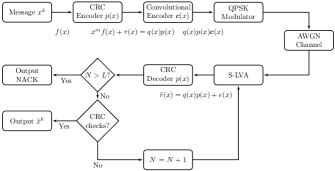
Figure 1: Block diagram of a system employing convolutional codes, CRC codes and S-LVA decoder

II System Model

The system model we study in this paper is shown in Fig. 1. A transmitter uses a CC and a CRC code to transmit an information sequence as follows: Let $f(x)$ denote a $k$-bit binary information sequence and $p(x)$ denote a degree-$m$ CRC generator polynomial. Let $r(x)$ denote the remainder when $x^{m}f(x)$ is divided by $p(x)$. First, the CRC polynomial is used to obtain the $n=k+m$-bit sequence $x^{m}f(x)+r(x)=q(x)p(x)$. The transmitter then uses a feedforward, rate-$\frac{1}{N}$ CC with $v$ memory elements and a generator polynomial $\bm{c}(x)$ to encode the $n$-bit sequence. The output $q(x)p(x)\bm{c}(x)$ of the convolutional encoder is transmitted over an additive white Gaussian noise (AWGN) channel using quadrature phase-shift keying (QPSK) modulation.

The receiver feeds the noisy received sequence into a S-LVA decoder with list size $L$ that identifies $L$ most likely $n$-bit input sequences sequentially. That is, S-LVA begins by finding the closest codeword $c_{1}$ to the received sequence and passing it to the CRC code for verification. If the CRC check fails, S-LVA outputs the next closest codeword $c_{2}$ and repeats the above procedure until the CRC check is successful or the best $L$ codewords $c_{1},\ldots c_{L}$ all fail the CRC check, in which case the decoder declares erasure and a NACK is generated.

In this paper, unless otherwise stated, the CRC code in the system model is the one designed using the CRC code search algorithm in [4] for the given convolutional code, in which the authors also provide the analytical upper bound on the undetected error probability with two different methods, the exclusion method and the construction method. We refer interested readers to [4] for more details.

III S-LVA Performance Analysis

From Sec. II, it can be seen that the failure rate of S-LVA can be expressed as

$$\operatorname{P}^{L}_{\operatorname{F}}=\operatorname{P}^{L}_{\operatorname{UE}}+\operatorname{P}^{L}_{\operatorname{NACK}},$$ (1)

where $\operatorname{P}^{L}_{\operatorname{UE}}$ and $\operatorname{P}^{L}_{\operatorname{NACK}}$ are both a function of SNR and list size $L$. The performance metrics of S-LVA include $\operatorname{P}^{L}_{\operatorname{F}}$, $\operatorname{P}^{L}_{\operatorname{UE}}$, $\operatorname{P}^{L}_{\operatorname{NACK}}$, and $\mathbb{E}[N_{\operatorname{LVA}}]$. In fact, $\operatorname{P}^{L}_{\operatorname{UE}}$ and $\operatorname{P}^{L}_{\operatorname{NACK}}$ reflect the overall characteristics of the coded channel model introduced in Sec. I-B as the coded channel requires the complete knowledge of transition probabilities from the transmitted codeword to the decoded codeword or NACK. Therefore it is important to understand how the SNR and list size $L$ affect $\operatorname{P}^{L}_{\operatorname{UE}}$ and $\operatorname{P}^{L}_{\operatorname{NACK}}$, respectively.

III-A S-LVA Performance vs. SNR

This section examines S-LVA performance as a function of SNR ($E_{s}/N_{0}$). The extreme cases of SNR (very low and very high) and list size ($L=1$ and $L={|{\cal C}|}$) are given particular attention as they frame the overall performance landscape.

In the discussion below, certain sets of codewords are important to consider. First, ${\cal C}$ is the set of all convolutional codewords. Since we consider a finite blocklength system where there are $n$ message bits and $v$ termination bits (completely determined by the $n=k+m$ message bits) fed into the convolutional encoder, the size of $\mathcal{C}$ is

$$|{\cal C}|=2^{n}=2^{k+m}.$$ (2)

Let $c^{*}$ denote the transmitted codeword. A superscript of $-$ indicates a set that excludes $c^{*}$. For example ${\cal C}^{-}$ is the set of all convolutional codewords except the transmitted codeword $c^{*}$. The set ${\cal C}_{\operatorname{CRC}}$ is the set of all convolutional codewords whose corresponding input sequences pass the CRC check. The size of ${\cal C}_{\operatorname{CRC}}$ is

$$|{\cal C}_{\operatorname{CRC}}|=2^{n-m}=2^{k}.$$ (3)

The set ${\cal C}_{\overline{{\operatorname{CRC}}}}$ is the set of all convolutional codewords whose corresponding input sequences do not pass the CRC check. The size of this set is

$$|{\cal C}_{\overline{{\operatorname{CRC}}}}|=2^{n}-2^{k}.$$ (4)

III-A1 The Case of $L={|{\cal C}|}$

Consider S-LVA with the largest possible list size $L={|{\cal C}|}$. Regardless of SNR, $\operatorname{P}^{|{\cal C}|}_{\operatorname{NACK}}=0$ always holds because S-LVA with $L={|{\cal C}|}$ will always find a codeword that passes the CRC check. Let $A_{d}$ be the number of distinct UEs of distance $d$ with positions taken into account. The UE probability $\operatorname{P}^{|{\cal C}|}_{\operatorname{UE}}$ is upper bounded by the union bound that some codeword in ${\cal C}_{\operatorname{CRC}}^{-}$ is pairwise more likely than $c^{*}$:

$$\operatorname{P}^{|{\cal C}|}_{\operatorname{UE}}\leq\sum_{c\in{\cal C}_{\operatorname{CRC}}^{-}}\operatorname{P}(d(c,c^{*})),$$ (5)

where $d(c,c^{*})$ is the distance between $c$ and $c^{*}$, and $\operatorname{P}(d(c,c^{*}))$ is the pairwise error probability of an error event with distance $d$. For QPSK modulation over the AWGN channel, $\operatorname{P}(d)$ can be computed using the Gaussian Q-function:

$$\operatorname{P}(d)=\operatorname{Q}(\sqrt{d\gamma_{s}})\leq\operatorname{Q}(\sqrt{\operatorname{\mathit{d}_{free}}\gamma_{s}})e^{-(d-\operatorname{\mathit{d}_{free}})\gamma_{s}/2},$$ (6)

where $\gamma_{s}=E_{s}/N_{0}$ is the signal-to-noise ratio (SNR) of a QPSK symbol, and $E_{s}$ and $N_{0}/2$ denote the energy per transmitted QPSK symbol and one-dimensional noise variance, respectively. .

Here, we point out that (5) is precisely the union bound of [4] given as an upper bound on $\operatorname{P}^{1}_{\operatorname{UE}}$. That it is also a valid upper bound for $\operatorname{P}^{|{\cal C}|}_{\operatorname{UE}}$ indicates that, at least at low SNR, this bound will be loose for $L=1$. At very low SNR, $\operatorname{P}^{|{\cal C}|}_{\operatorname{UE}}$ converges to $\frac{|{\cal C}_{\operatorname{CRC}}^{-}|}{|{\cal C}_{\operatorname{CRC}}|}\approx 1$. We refer the reader to [4] for the exact expression of the union bound.

For $k=256$ bits, Fig. 2 shows $\operatorname{P}^{|{\cal C}|}_{\operatorname{UE}}$ as a function of $E_{s}/N_{0}$ for the $(13,17)$ CC using soft Viterbi decoding without a CRC code and S-LVA with $L=|{\cal C}|$ combined with the optimal degree-$6$ CRC code 0x43. The truncated union bound at $\tilde{d}=24$ on $\operatorname{P}^{|{\cal C}|}_{\operatorname{UE}}$ of (5) derived via exclusion method in [4] is also shown. It can be seen that the union bound on $\operatorname{P}^{|{\cal C}|}_{\operatorname{UE}}$ becomes tight as SNR increases.

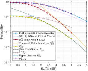
Figure 2: Comparison of FER between S-LVA combined with the optimal degree-$6$ CRC code 0x43 and soft Viterbi decoding (without a CRC code) for $(13,17)$ CC when $n=256+6$ bits. $(261,\ 6)$ NNA on soft Viterbi decoding, truncated union bound at $\tilde{d}=24$ on $\operatorname{P}_{\operatorname{UE}}^{|\mathcal{C}|}$, conjecture of $2^{-6}\operatorname{P}_{\operatorname{F}}^{1}$, upper limit of $2^{-6}$, and $(668,\ 12)$ NNA on $\operatorname{P}_{\operatorname{UE}}^{1}$ are also provided as a reference.

III-A2 The Case of $L=1$

For $L=1$, with the same blocklength $n$, $\operatorname{P}^{1}_{\operatorname{F}}$ is exactly the FER of the CC under soft Viterbi decoding with no CRC code. The addition of the CRC code separates the failures into erasures and UEs, with probabilities $\operatorname{P}^{1}_{\operatorname{NACK}}$ and $\operatorname{P}^{1}_{\operatorname{UE}}$, respectively. Thus we have union bounds, nearest neighbor approximation (NNA), and a low-SNR upper limit as follows:

$$\operatorname{P}^{1}_{\operatorname{NACK}} \leq\sum_{c\in{\cal C}_{\overline{{\operatorname{CRC}}}}}\operatorname{P}(d(c,c^{*}))$$ (7)

$$\approx A_{\operatorname{\mathit{d}_{free}}}\operatorname{P}(\operatorname{\mathit{d}_{free}}),$$ (8)

$$\operatorname{P}^{1}_{\operatorname{UE}} \leq\sum_{c\in{\cal C}_{\operatorname{CRC}}^{-}}\operatorname{P}(d(c,c^{*}))$$ (9)

$$\approx A_{\operatorname{\mathit{d}_{CRC}}}\operatorname{P}(\operatorname{\mathit{d}_{CRC}}),$$ (10)

$$\lim_{\gamma_{s}\to-\infty}\operatorname{P}^{1}_{\operatorname{UE}}=2^{-m},$$ (11)

where $A_{d}$ denotes the number of distinct UEs at distance $d$ with positions taken into account.

Note that (9) is identical to (5), but $\operatorname{P}^{1}_{\operatorname{UE}}$ should be significantly smaller than $\operatorname{P}^{|{\cal C}|}_{\operatorname{UE}}$. Thus we propose an improved bound on $\operatorname{P}^{1}_{\operatorname{UE}}$ as follows: for a randomly chosen degree-$m$ CRC code and $L=1$ we expect an incorrectly chosen convolutional codeword to pass the CRC check with probability $2^{-m}$. This should be an upper bound on the performance of CRCs optimized according to [4]. Thus we conjecture that

$$\operatorname{P}^{1}_{\operatorname{UE}} \leq 2^{-m}\operatorname{P}^{1}_{\operatorname{F}}\,.$$ (12)

This upper bound should be loose for well-designed CRCs at high SNR. However, at very low SNR we expect this bound to be tight based on the fact that the upper limit of $\operatorname{P}_{\operatorname{UE}}^{1}$ satisfies (11). Fig. 2 shows that (12) is accurate at very low SNR and the NNA of $\operatorname{P}_{\operatorname{UE}}^{1}$ in (10) is quite accurate at high SNR. The parameters of the NNA are $A_{\operatorname{\mathit{d}_{CRC}}}=668$ and $\operatorname{\mathit{d}_{CRC}}=12$.

III-B Complexity Analysis of S-LVA

In [9], the authors present tables that compare the time and space complexity for different implementations of the LVA. Although the multiple-list tree-trellis algorithm (ml-TTA) achieves linear time complexity for the backward passes of the S-LVA, the implementation does not support floating point precision without the use of quanitization. The T-TTA is another implementation of the S-LVA that uses a red-black tree to store the cumulative metric differences during a traceback operation. Their time complexity results indicate that the T-TTA achieve the best performance for algorithms that support floating point precision. The analysis of the S-LVA in this assumes the use of the T-TTA.

For a fixed blocklength and a specified CC-CRC pair, the decoding complexity of S-LVA depends mainly on the number of decoding trials performed. Denote by $N_{\operatorname{LVA}}$ the random variable indicating the number of decoding trials of S-LVA for a received codeword randomly drawn according to the noise distribution. First, we show that with list size $|\mathcal{C}|$, the expected value of $N_{\operatorname{LVA}}$, $\mathbb{E}[N_{\operatorname{LVA}}]$, converges to $1$ as SNR increases and converges to $2^{m}(1-\epsilon)$, for a small $\epsilon>0$ as SNR decreases. Next, we prove that $N_{\operatorname{LVA}}$ is a bounded random variable where the upper bound is approximately the number of all possible convolutional codes within $d_{\operatorname{CRC}}$. Finally, we measure the complexity of S-LVA by the time ratio, which is the ratio of the actual time an insertion or traceback operation consumes to the actual time a standard Viterbi algorithm consumes, which is the complexity of add-compare-select (ACS) operations in trellis building plus one traceback operation.

Theorem 1

The expected number of decoding trials $\mathbb{E}[N_{\operatorname{LVA}}]$ for S-LVA with list size $|\mathcal{C}|$, used with a degree-$m$ CRC code, satisfies (i) $\lim_{\gamma_{s}\to\infty}\mathbb{E}[N_{\operatorname{LVA}}]=1$; (ii) $\lim_{\gamma_{s}\to-\infty}\mathbb{E}[N_{\operatorname{LVA}}]=2^{m}(1-\epsilon)$, where $\epsilon\to 0$ as $n\to\infty$.

Proof:

Let $\tilde{x}_{i}^{n}$ denote the $i^{\text{th}}$ output of the S-LVA, which is the codeword at position $i$ in the list of all possible codewords sorted according to increasing soft Viterbi metric (typically Hamming or Euclidean distance) with respect to the received noisy codeword.

(i) Consider the event $A_{i}\triangleq\cap_{j=1}^{i-1}\{p(x)\nmid\tilde{x}^{n}_{j}\}\cap\{p(x)\mid\tilde{x}^{n}_{i}\},$ where $p(x)$ is the CRC polynomial. Because of the existence of codewords that have $p(x)$ as a factor (i.e. that pass the CRC check), there exists a maximum decoding depth $\tilde{N}<\infty$ such that $\Pr\{A_{j}\}=0,\forall j>\tilde{N}$.

Note that when $\gamma_{s}\to\infty$, $\Pr\{A_{1}\}\to 1$ and $\sum_{i=2}^{\tilde{N}}\Pr\{A_{i}\}\to 0$. Thus,

$$\lim_{\gamma_{s}\to\infty}\mathbb{E}[N_{\operatorname{LVA}}] =\lim_{\gamma_{s}\to\infty}\left[1\cdot\Pr\{A_{1}\}+\sum_{i=2}^{\infty}i\Pr\{A_{i}\}\right]$$

$$=\lim_{\gamma_{s}\to\infty}\left[1\cdot\Pr\{A_{1}\}+\sum_{i=2}^{\tilde{N}}i\Pr\{A_{i}\}\right]$$

$$\leq\lim_{\gamma_{s}\to\infty}\left[1\cdot\Pr\{A_{1}\}+\tilde{N}\sum_{i=2}^{\tilde{N}}\Pr\{A_{i}\}\right]$$

$$=1.$$ (13)

Since $N_{\operatorname{LVA}}\geq 1$, $\mathbb{E}[N_{\operatorname{LVA}}]\geq 1$. It follows that $\lim_{\gamma_{s}\to\infty}\mathbb{E}[N_{\operatorname{LVA}}]=1$.

(ii) When $\gamma_{s}\to-\infty$, the SNR is low enough such that with high probability the received sequence $\bm{y}$ is far away from the entire constellation of all possible sequences that can be transmitted in $\mathbb{R}^{n}$. This implies that with very high probability $\bm{y}$ is almost equidistant from all possible convolutional codewords that can be transmitted. For those received sequences almost equidistant from all convolutional codewords, the S-LVA decoding process can be modeled as follows: In a basket of ”blue” balls (codewords that pass the CRC check) and ”red” balls (codewords that do not pass the CRC check), the S-LVA chooses balls at random without replacement with the objective of stopping when it successfully picks a blue ball. Thus, $\mathbb{E}[N_{\operatorname{LVA}}]$ can be computed using a standard result in combinatorics as follows. For a decoded sequence with $n$ message and parity-check bits and $v$ trailing zero bits, the total number of balls in the basket is $N=2^{n}$ and the number of blue balls in the basket is $M=2^{n-m}$:

$$\lim_{\gamma_{s}\to-\infty}\mathbb{E}[N_{\operatorname{LVA}}] =1+\frac{N-M}{M+1}$$

$$=\frac{N+1}{M+1}$$

$$=2^{m}\left[1-\frac{2^{m}-1}{2^{m}+2^{n}}\right]$$

$$=2^{m}(1-\epsilon),$$ (14)

where $\epsilon=\frac{2^{m}-1}{2^{m}+2^{n}}>0$. When $m$ is fixed, $\lim_{n\to\infty}\mathbb{E}[N_{\operatorname{LVA}}]=2^{m}$. ∎

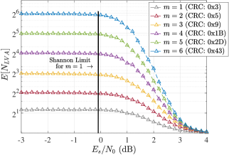
Figure 3: $\mathbb{E}[N_{\operatorname{LVA}}]$ vs. $E_{s}/N_{0}$ of degree $1-6$ optimal CRC codes for $(13,17)$ CC, with $k=256$.

Fig. 3 shows empirical $\mathbb{E}[N_{\operatorname{LVA}}]$ for the $(13,17)$ CC with the optimal CRC codes with degrees ranging from $1$ to $6$ when $k=256$ bits. The curves verify Theorem 1; $\mathbb{E}[N_{\operatorname{LVA}}]\to 1$ as the SNR increases and $\mathbb{E}[N_{\operatorname{LVA}}]\approx 2^{m}$ as the SNR decreases to very low values. While the result we have obtained in Theorem 1 for the case of $\gamma_{s}\to-\infty$ requires very low SNR values for the arguments made to hold, it is interesting to see from the figure that S-LVA behaves similar to random guessing as soon as the SNR value is below the Shannon limit, shown as a vertical line for $m=1$. (The limits for the other values of $m$ are very close to the limit for $m=1$).

Theorem 1 studies the limit of $\mathbb{E}[N_{\operatorname{LVA}}]$ in the limit of extremely high and low SNR regimes. In practice, SNRs ranging between 0.5 dB and 4 dB above the Shannon limit are of particular interest. As shown in Fig. 3, $\mathbb{E}[N_{\operatorname{LVA}}]$ traverses its full range from $\approx 2^{m}$ to $1$ in this range of practical interest.

Theorem 2

The number of decoding attempts of S-LVA with list size $L=|\mathcal{C}|$, $N_{\operatorname{LVA}}$, is upper bounded by

$$N_{\operatorname{LVA}}\leq\sum_{d=\operatorname{\mathit{d}_{free}}}^{d_{\operatorname{CRC}}}B_{d}-A_{d_{\operatorname{CRC}}}+1,$$ (15)

where $B_{d}$ denotes the number of all possible CCs with distance $d$, and $A_{d_{\operatorname{CRC}}}$ denotes the number of UEs with distance $d_{\operatorname{CRC}}$, both with positions taken into account.

Proof:

Since the Gaussian noise is independent of the transmitted codeword, the all-zero CC can always be thought of as the transmitted CC and the surrounding CCs are the error events. Since all-zero message sequence can already pass the CRC check. The upper bound can be obtained by finding the maximum number of codewords until S-LVA finds the second CC whose input sequence can pass the CRC check.

Now consider the following extreme case: First, if S-LVA decode $S$ times, where $S=\sum_{d=\operatorname{\mathit{d}_{free}}}^{d_{\operatorname{CRC}}}B_{d}$, it certainly can hit a CC whose input codeword checks the CRC, since $S$ trials will include the undetectable nearest neighbors of all-zero CC. Note that here, the undetectable nearest neighbors are the relative constellation points of the true nearest neighbors of the transmitted CC. Thus by subtracting the number of undetectable nearest neighbors and then adding back one undetectable nearest neighbor, we know that the S-LVA will terminate as well by decoding at most $S-N+1$ times, which concludes that $S-N+1$ is a valid upper bound. ∎

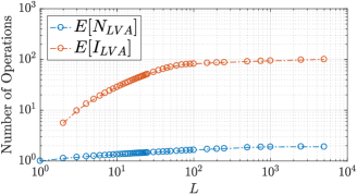
Figure 4: The expected number $\mathbb{E}[N_{\operatorname{LVA}}]$ of decoding attempts and expected number $\mathbb{E}[I_{\operatorname{LVA}}]$ of insertions performed with different list sizes for $(27,31)$ CC, and 0x709 CRC code, with $k=64$ at $2$ dB. In the simulaiton setting, $C_{1}=1.5$ and $C_{2}=2.2$.

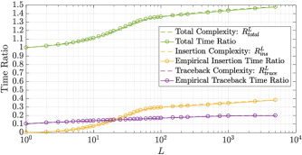
Figure 5: The complexity of S-LVA with different list sizes for $(27,31)$ CC, and 0x709 CRC code, with $k=64$ at $2$ dB. In the simulaiton setting, $C_{1}=1.5$ and $C_{2}=2.2$.

Theorem 2 shows that the number of decoding attempts of S-LVA is a bounded random variable, which means that it is enough to set list size $L=\sum_{d=\operatorname{\mathit{d}_{free}}}^{d_{\operatorname{CRC}}}B_{d}-A_{d_{\operatorname{CRC}}}+1$ which is far less than $|\mathcal{C}|$.

Although the complexity of S-LVA is determined by $\mathbb{E}[N_{\operatorname{LVA}}]$, still, it would be interesting to investigate how time complexity changes as list size $L$ varies. Here, we define the complexity metric of S-LVA as the time ratio $R^{L}_{total}$, which is the ratio of the actual time an insertion or traceback operation consumes to the actual time a standard Viterbi algorithm consumes. This metric provides a quantititive measure on the time consumption any other steps in the algorithm would cost compared to that of a standard Viterbi algorithm.

Note that S-LVA mainly comprises two steps: an ACS operation and multiple tracebacks where the multiple tracebacks require a dynamic sorted list to obtain the next position of detour state on trellis. Thus, the time complexity of multiple tracebacks can be further split into the complexity of obtaining one trellis path and the complexity of insertions required to maintain the sorted list. When list size is large, both complexities can be seen as independent.

Let $R_{trace}^{L}$ denote the time ratio of retrieving a single trellis path and $R_{ins}^{L}$ denote the time ratio of insertions, we have

$$R_{total}^{L}=1+R_{trace}^{L}+R_{ins}^{L},$$ (16)

in which

$$N_{\operatorname{Viterbi}}= (2+1)(k+m-v)2^{v}+2\sum_{i=1}^{v}2^{i}+\sum_{i=0}^{v-1}2^{i}$$ (17)

$$+C_{1}\cdot\left[2(k+m+v)+1.5(k+m)\right]$$ (18)

$$= 5(2^{v}-1)+3(k+m-v)\cdot 2^{v}$$

$$+C_{1}\cdot\left[2(k+m+v)+1.5(k+m)\right],$$ (19)

$$R_{trace}^{L}= \frac{\mathbb{E}[N_{\operatorname{LVA}}]\cdot C_{1}\cdot\left[2(k+m+v)+1.5(k+m)\right]}{N_{\operatorname{Viterbi}}},$$ (20)

$$R_{ins}^{L}= \frac{\mathbb{E}[I_{\operatorname{LVA}}]\cdot C_{2}\cdot\log(\mathbb{E}[I_{\operatorname{LVA}}])}{N_{\operatorname{Viterbi}}},$$ (21)

where $C_{1},C_{2}$ are two hardware specific constants, $\mathbb{E}[N_{\operatorname{LVA}}]$ denotes the expected number of decoding attempts and $\mathbb{E}[I_{\operatorname{LVA}}]$ denotes the expected number of insertions to maintain a sorted list. The denominator $N_{\operatorname{Viterbi}}$ indicates the number of operations required for a standard ACS operation.

Fig. 4 shows the expected number of decoding attempts versus list size $L$ and the expected number of insertions to maintain a sorted list versus list size $L$ for $(27,31)$ CC, 0x709 CRC code with $k=64$ at 2 dB. Fig. 5 shows the time ratio of S-LVA as a function of list size $L$. It can be seen that (20) and (21) match the empirical time ratio of traceback operations and insertion operation with high accuracy. Though the degree of 0x709 CRC code is 10, one can observe that the overall time ratio is still comparable to that of a standard Viterbi algorithm, which indicates that using a strong CRC code may not necessarily lead to a huge complexity increase, as long as the CC-CRC pair is operated in the optimal SNR range.

III-C S-LVA Performance vs. $L$

As we learned in Sec. III-A1, the “complete” S-LVA algorithm with $L={|{\cal C}|}$ achieves $\operatorname{P}^{|{\cal C}|}_{\operatorname{NACK}}=0$ and $\operatorname{P}^{|{\cal C}|}_{\operatorname{UE}}$ is well approximated by truncating the union bound of (5) at a reasonable $\tilde{d}$. In the context of a feedback communication system, it is often preferable to retransmit a codeword or to lower the rate of the transmission through incremental redundancy rather than to accept undetectable errors. Thus the full complexity $L={|{\cal C}|}$ may actually lead to detrimental results in certain cases, especially at very low SNRs where $\operatorname{P}^{|{\cal C}|}_{\operatorname{UE}}$ approaches 1.

Sec. III-A2 showed how the other extreme of $L=1$ significantly lowers the UE probability with $\operatorname{P}^{1}_{\operatorname{UE}}$ well approximated by the minimum between the upper bound of (12) and the NNA of (10). The reduction in $\operatorname{P}_{\operatorname{UE}}$ comes at the cost of a significantly increased $\operatorname{P}^{1}_{\operatorname{NACK}}$, which is approximately the FER of the CC decoded by soft Viterbi without a CRC code.

We expect the best choice of $L$ for many systems to be in between these two extremes. The rest of this section explores how $\operatorname{P}^{L}_{\operatorname{UE}}$ and $\operatorname{P}^{L}_{\operatorname{NACK}}$ vary with $L$. In general, with SNR fixed, $\operatorname{P}_{\operatorname{NACK}}^{L}$ and $\operatorname{P}_{\operatorname{UE}}^{L}$ have the following properties: $\operatorname{P}_{\operatorname{NACK}}^{L}$ is a decreasing function of $L$ with $\lim_{L\to|\mathcal{C}|}\operatorname{P}_{\operatorname{NACK}}^{L}=0$, and $\operatorname{P}_{\operatorname{UE}}^{L}$ is an increasing function of $L$ with $\lim_{L\to|\mathcal{C}|}\operatorname{P}_{\operatorname{UE}}^{L}=\operatorname{P}^{|\mathcal{C}|}_{\operatorname{UE}}$, which is well approximated by (5).

Therefore, one could ask what the optimal list size $L^{*}$ is such that, for example, $\operatorname{P}_{\operatorname{NACK}}^{L}\leq\operatorname{P}_{\operatorname{NACK}}^{*}$ and $\operatorname{P}_{\operatorname{UE}}^{L}\leq\operatorname{P}_{\operatorname{UE}}^{*}$, where $\operatorname{P}_{\operatorname{NACK}}^{*}$ and $\operatorname{P}_{\operatorname{UE}}^{*}$ are target erasure and UE probabilities, respectively. We present useful bounds on $\operatorname{P}_{\operatorname{NACK}}^{L}$ and $\operatorname{P}_{\operatorname{UE}}^{L}$ to further explore the concept of an optimal list size $L^{*}$.

Corollary 1 (Markov bound on $\operatorname{P}_{\operatorname{NACK}}^{L}$)

The erasure probability $\operatorname{P}_{\operatorname{NACK}}^{L}$ satisfies $\operatorname{P}_{\operatorname{NACK}}^{L}\leq\frac{1}{L}$ if $\gamma_{s}\to\infty$.

Proof:

The result is a direct consequence of Markov inequality. The erasure probability with a list size $L$ is given as $\operatorname{P}_{\operatorname{NACK}}^{L}=\Pr\{N_{\operatorname{LVA}}>L\}$, where $N_{\operatorname{LVA}}$ is the random variable representing the decoding trial at which the CRC check first passes. By applying Markov inequality for $\gamma_{s}\to\infty$, we have

$$\operatorname{P}_{\operatorname{NACK}}^{L}=\Pr\{N_{\operatorname{LVA}}>L\}\leq\frac{\mathbb{E}[N_{\operatorname{LVA}}]}{L}=\frac{1}{L}.$$ (22)

∎

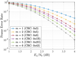
Figure 6: FER vs. $E_{s}/N_{0}$ of degree $1-6$ optimal CRC codes for $(13,17)$ CC with $k=256$.

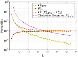
Figure 7: Trade-off between $\operatorname{P}_{\operatorname{NACK}}^{L}$ and $\operatorname{P}_{\operatorname{UE}}^{L}$ for the optimal degree-$5$ CRC code 0x2D and $(13,17)$ CC when $k=256,\ \gamma_{s}=3.7$ dB.

A more useful Chebyshev bound on $\operatorname{P}_{\operatorname{NACK}}^{L}$ could be obtained if one knows the variance $\operatorname{var}(N_{\operatorname{LVA}})$ at high SNR.

Corollary 2 (Chebyshev bound on $\operatorname{P}_{\operatorname{NACK}}^{L}$)

Given $\operatorname{var}(N_{\operatorname{LVA}})$ at $\gamma_{s}\gg 0$, $\operatorname{P}_{\operatorname{NACK}}^{L}$ satisfies $\operatorname{P}_{\operatorname{NACK}}^{L}\leq\frac{\operatorname{var}(N_{\operatorname{LVA}})}{(L-1)^{2}}$, where $L\geq 2$.

Proof:

The result is a direct consequence of Chebyshev inequality. Since $\gamma_{s}\gg 0$, $\mathbb{E}[N_{\operatorname{LVA}}]\to 1$. From Chebyshev inequality, we have

$$\operatorname{P}_{\operatorname{NACK}}^{L} =\Pr\{N_{\operatorname{LVA}}>L\}$$

$$=\Pr\{N_{\operatorname{LVA}}\geq L+1\}$$

$$\leq\Pr\{|N_{\operatorname{LVA}}-\mathbb{E}[N_{\operatorname{LVA}}]|\geq L-\mathbb{E}[N_{\operatorname{LVA}}]+1\}$$

$$\leq\frac{\operatorname{var}(N_{\operatorname{LVA}})}{(L-(\mathbb{E}[N_{\operatorname{LVA}}]-1))^{2}}$$

$$\leq\frac{\operatorname{var}(N_{\operatorname{LVA}})}{(L-1)^{2}}.$$ (23)

∎

As an example, we study the trade-off between $\operatorname{P}_{\operatorname{NACK}}^{L}$ and $\operatorname{P}_{\operatorname{UE}}^{L}$ for the $(13,17)$ CC. Assume at $\gamma_{s}=3.7$ dB, $\operatorname{P}_{\operatorname{NACK}}^{*}=10^{-3}$ and $\operatorname{P}_{\operatorname{UE}}^{*}=8\times 10^{-4}$. In Fig. 6, the FER of degree $1-6$ optimal CRC codes is plotted. Here we use the optimal degree-$5$ CRC code with the $(13,17)$ CC to illustrate how to find the optimal list size $L^{*}$. Fig. 7 shows the trade-off between $\operatorname{P}_{\operatorname{NACK}}^{L}$ and $\operatorname{P}_{\operatorname{UE}}^{L}$ when $k=256$ at $3.7$ dB. It can be seen that $L^{*}=8$ satisfies $\operatorname{P}_{\operatorname{NACK}}^{L}\leq\operatorname{P}_{\operatorname{NACK}}^{*}$ and $\operatorname{P}_{\operatorname{UE}}^{L}\leq\operatorname{P}_{\operatorname{UE}}^{*}$.

If $\operatorname{P}_{\operatorname{NACK}}^{*}=10^{-3}$, $\operatorname{P}_{\operatorname{UE}}^{*}=10^{-3}$ and empirical $\operatorname{var}(N_{\operatorname{LVA}})=0.2823$ is known, since $\operatorname{P}_{\operatorname{UE}}^{L}\leq\operatorname{P}_{\operatorname{UE}}^{*}$ always holds, one can directly apply the empirical Chebyshev bound to obtain $L^{*}\geq 18$ without knowing the true $\operatorname{P}_{\operatorname{NACK}}^{L}$ curve.

IV Coded Channel and Its Capacity

In Sec. III, we have thoroughly discussed the performance of S-LVA combined with the optimal CRC code designed specifically for the given CC, in which the decoding complexity depends mainly on the expected number of decoding attempts. One important observation is that, with SNR in a relatively high regime, this expected number is much less than $2^{m}(1-\epsilon)$, where $\epsilon>0$ is a small constant, which suggests that the decoding can be done much more efficiently. Still, different CC-CRC pair corresponds to different decoding compleixty. Therefore, a more general question to ask is that, how to select the optimal CC-CRC pair for the system model introduced in Sec. II. We propose the coded channel model to address this problem.

Figure 8: Block diagram of the equivalent coded channel

IV-A The Coded Channel Model

The equivalent coded channel model of the system model introduced in Sec. II is shown in Fig. 8, which consists of two finite sets $\mathcal{X}$ and $\mathcal{Y}$ and a channel matrix $P$, where $\mathcal{X}$ denotes the set of all possible $k$-bit message sequences with $|\mathcal{X}|=2^{k}$, $\mathcal{Y}=\mathcal{X}\cup\{E\}$ with $|\mathcal{Y}|=2^{k}+1$ and the channel matrix $P$ is a single equivalent abstraction of the CRC encoder, the convolutional encoder, the AWGN channel, the S-LVA decoder and the CRC decoder in Fig. 1. To make the coded channel complete, we introduce the “outer” message encoder which simply selects the $W$-th message symbol $X(W)$ in $\mathcal{X}$ and the “outer” message decoder which simply decodes message symbol $Y(\hat{W})$ to the $\hat{W}$-th message, where $W\in\{1,2,\cdots,2^{k}\}$ and $\hat{W}\in\{1,2,\cdots,2^{k},2^{k}+1\}$ are both indices. If $W=\hat{W}$, then $X(W)=Y(\hat{W})$ and vice versa. If $Y(\hat{W})=E$, then $\hat{W}=2^{k}+1$.

Obviously, if one knows each transition probability from $X^{k}$ to $Y^{k}$ and $X^{k}$ to $E$, then the entire part from the CRC encoder to CRC decoder shown in Fig. 1 can be equivalently substituted with a single channel $P$ and the corresponding coded channel capacity $C(P)$, which indicates the maximum bits per codeword transmission, can be computed.

For brevity, define $\epsilon\triangleq P^{L}_{\operatorname{UE}}$ and $\alpha\triangleq P^{L}_{\operatorname{NACK}}$ which indicate the overall characteristics of the coded channel $P$. Unless otherwise stated, we will keep this notation in the following sections. We first show that $P$ is a symmetric channel.

Theorem 3

The equivalent coded channel matrix $P$ of the CRC encoder, the convolutional encoder, the AWGN channel, the S-LVA decoder, and the CRC decoder, is a symmetric channel, and the coded channel capacity $C(P)$ is achieved by the uniform distribution.

Proof:

Let us partition $P$ into $P=[Q\mid\alpha I]$ where $\alpha\triangleq\operatorname{P}^{L}_{\operatorname{NACK}}$, $Q$ denotes a $2^{k}\times 2^{k}$ matrix, and $I$ is a $2^{k}\times 1$ all-one matrix. It can be shown that $P$ satisfies the following properties:

• $Q=Q^{T}$ due to the linearity of the convolutional code;

• Rows in $Q$ are permutations of each other, which is due to the independence of the Gaussian noise on the transmitted codeword;

• Columns in $Q$ are permutations of each other, which is a direct consequence of (i) and (ii).

Since $\alpha I$ also satisfies (ii) and (iii). Therefore $P=[Q\mid\alpha I]$ is a symmetric channel and the capacity is achieved by the uniform distribution. ∎

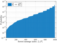
Figure 9: A typical stair-shaped of probability distribution of the unknown probabilities with $(13,17)$ CC, a degree-$6$ CRC code 0x43, $k=10$ and S-LVA with $L=|\mathcal{C}|$ at $0$ dB when transmitted convolutional code is the all-zero codeword. Some zero unknown probabilities are omitted due to the insufficient number of simulations.The highest level corresponds to the probability of decoding to nearest neighbors of the transmitted all-zero convolutional code.

IV-B True Coded Channel

In practice, it is difficult to completely determine each entry of $P$, especially when $k$ is large. Therefore let the unknown probabilities be specified as $p_{1},p_{2},\cdots,p_{2^{k}-1}$ with $p_{i}\geq 0$ and $\sum_{i=1}^{2^{k}-1}p_{i}=\epsilon$, for each transmitted message. Thus, the true coded channel capacity $C(P)$ can be computed when $p(x)$ is uniformly distributed

$$C(P)= H(Y)-H(Y|X=x(w))$$ (24)

$$= H_{2^{k}+1}\left(\frac{1-\alpha}{2^{k}},\cdots,\frac{1-\alpha}{2^{k}},\alpha\right)$$

$$-H_{2^{k}+1}(1-\epsilon-\alpha,\alpha,p_{1},p_{2},\cdots,p_{2^{k}-1})$$ (25)

$$= (1-\alpha)\left[k-H\left(\frac{\epsilon}{1-\alpha}\right)\right]$$

$$-\epsilon H_{2^{k}-1}\left(\frac{p_{1}}{\epsilon},\frac{p_{2}}{\epsilon},\cdots,\frac{p_{2^{k}-1}}{\epsilon}\right),$$ (26)

where $x(w)$ is some fixed message symbol in $\mathcal{X}$.

Now that the true coded channel is a much complicated model, still, there are some intuitions that can be drawn from this model. As an example, Fig. 9 shows the sorted probability distribution of the unknown probabilities $p_{1},p_{2},\cdots,p_{2^{k}-1}$ for $k=10$, which demonstrates a stair-shaped envelop. The highest level corresponds to the probabilities of decoding to the nearest neighbors of the transmitted convolutonal codeword. As SNR increases, the bulk of probability of error will move towards nearest neighbors, which suggests that nearest neighbors might be a useful tool to approximate the true coded channel capacity.

To formally present the above intuitions, we propose the following three simplied coded channel models which only require the knowlege of $\epsilon$, $\alpha$ and the number of nearest neighbors of the transmitted message $N$ to approximate the true coded channel, which are referred to as loose lower bound model (LLB), nearest neighbor lower bound model (NNLB) and nearest neighbor upper bound model (NNUB).

IV-C Loose Lower Bound Model (LLB)

In this model, we assume that for each transmitted message symbol, the probability of decoding to the erasure symbol $E$ is $\alpha$ and the probabilities of decoding to message symbols other than the transmitted message are equally likely with $p_{i}=\frac{\epsilon}{2^{k}-1}$ for $i=1,2,\cdots,2^{k}-1$.

Similarly, the capacity $C(P_{\operatorname{LLB}})$ can be computed as

$$C(P_{\operatorname{LLB}})=(1-\alpha)\left[k-H\left(\frac{\epsilon}{1-\alpha}\right)\right]-\epsilon\log(2^{k}-1).$$ (27)

Obviously, $C(P_{\operatorname{LLB}})<C(P)$. The reason why this model becomes loose is that, except for the probability of decoding correctly or decoding to an erasure symbol, the rest of the probability is evenly allocated to message symbols other than the transmitted one. However in the true coded channel model, the nearest neighbors of the transmitted convolutional code will account for most of the rest probability since they are the closest codewords that S-LVA decodes to.

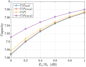
Figure 10: Capacity vs. SNR for LLB, NNLB, true coded channel, and NNUB model, with $k=8$, $m=6$, and $v=3$, in which $n_{c}=2(k+m+v)$ denotes the number of bits that are sent to the binary AWGN (Bi-AWGN) channel.

IV-D Nearest Neighbor Lower Bound Model (NNLB)

In this model, we assume that for each transmitted message symbol, the number of nearest neighbors $N\ (0<N<2^{k}-1)$ and the approximate probability of a single nearest neighbor $\epsilon^{*}$ are known. Here, $\frac{\epsilon}{2^{k}-1}<\epsilon^{*}<\frac{\epsilon}{N}$ since the nearest neighbors have the highest probability thus $\epsilon^{*}$ should be above the average. Thus, the remaining $2^{k}-1-N$ unknown probabilities will equally split probability $\epsilon-N\epsilon^{*}$. The capacity for this channel, $C(P_{\operatorname{NNLB}})$, can be computed as

$$C(P_{\operatorname{NNLB}})= (1-\alpha)\left[k-H\left(\frac{\epsilon}{1-\alpha}\right)\right]-\epsilon H\left(\frac{N\epsilon^{*}}{\epsilon}\right)$$

$$-N\epsilon^{*}\log N-(\epsilon-N\epsilon^{*})\log(2^{k}-1-N).$$ (28)

We point out that the NNLB model will awlays be a good approximation on the true coded channel capacity, since the nearest neighbors are taken into account which have the dominating unknown probabilities. As SNR increases, the nearest neighbors will be the most likely erroneously decoded codewords and codewords further away than nearest neighbors will be more unlikely. Therefore, we expect $C(P_{\operatorname{NNLB}})$ to approach $C(P)$ in high SNR regime. In fact, an extreme situation would be that $\epsilon$ only goes to the nearest neighbors, which gives rise to the following upper bound model.

IV-E Nearest Neighbor Upper Bound Model (NNUB)

In this model, we assume that for each transmitted message symbol, the number of nearest neighbors $N$ is known and probability of error $\epsilon$ is equally divided only by the nearest neighbors. That is, probability of each nearest neighbor is $\frac{\epsilon}{N}$ and codewords further away from nearest neighbors are unlikely. Thus, the capacity for this channel, $C(P_{\operatorname{NNUB}})$, can be computed as

$$C(P_{\operatorname{NNUB}})= (1-\alpha)\left[k-H\left(\frac{\epsilon}{1-\alpha}\right)\right]-\epsilon\log N.$$ (29)

IV-F Comparisons

The following theorem describes the relationships among the above four models.

Theorem 4

For a coded channel with message blocklength $k$, it holds that

$$C(P_{\operatorname{LLB}})<C(P_{\operatorname{NNLB}})<C(P)<C(P_{\operatorname{NNUB}})+\epsilon\log N,$$ (30)

provided that the $2^{k}-1$ unknown probabilities of each row in coded channel $P$ are distinct, $0<N<2^{k}-1$, and $\frac{\epsilon}{2^{k}-1}<\epsilon^{*}<\frac{\epsilon}{N}$.

Proof:

The chain of inequalities $C(P_{\operatorname{LLB}})<C(P_{\operatorname{NNLB}})<C(P)$ can be established by applying the fact that the uniform increases entropy to $H(Y|X=x(w))$. ∎

As an example, Fig. 10 illustrates the capacities for LLB channel, NNLB channel, true coded channel, and NNUB channel.

V Optimal CC-CRC Design

TABLE I: Most Popular Rate-$1/2$ Convolutional Codes and Corresponding Distance-Spectrum-Optimal CRC Codes with $k=64$

$v$	Conv. Code	Distance-Spectrum-Optimal CRC Generator Polynomial
		$m$	3	4	5	6	7	8	9	10
3	(13,17)		0x9	0x1B	0x2D	0x43	0xB5	0x107	0x313	0x50B
4	(27,31)		0xF	0x15	0x33	0x4F	0xD3	0x13F	0x2AD	0x709
5	(53,75)		0x9	0x11	0x25	0x49	0xEF	0x131	0x23F	0x73D
6	(133,171)		0xF	0x1B	0x23	0x41	0x8F	0x113	0x2EF	0x629
7	(247,371)		0x9	0x13	0x3F	0x5B	0xE9	0x17F	0x2A5	0x61D
8	(561,753)		0xF	0x11	0x33	0x49	0x8B	0x19D	0x27B	0x4CF
9	(1131,1537)		0xD	0x15	0x21	0x51	0xB7	0x1D5	0x20F	0x50D
10	(2473,3217)		0xF	0x13	0x3D	0x5B	0xBB	0x105	0x20D	0x6BB

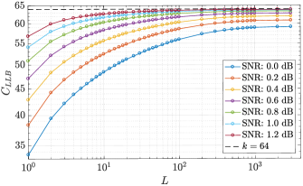
Figure 11: The coded channel capacity $C_{\operatorname{LLB}}$ in loose lower bound model vs. list size $L$ for $(247,371)$ CC and 0x61D CRC code.

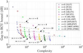
Figure 12: the SNR ($E_{s}/N_{0}$) gap to RCU bound vs. decoding complexity for various CC-CRC pairs with $k=64$ and target FER $10^{-3}$. Each color corresponds to a specific CC shown in parenthesis. Markers from top to bottom with the same color correspond to soft Viterbi decoding, $m=3,4,\cdots,10$ distance-spectrum-optimal CRC codes, respectively. CCs with $v=11,12,13$ using soft Viterbi decoding are also provided.

In this section, we present the design methodology and examples of optimal CC-CRC pairs under a target FER. Since the design of optimal list size $L$ is independent of the design of optimal CC-CRC pairs, we first show that $L=|\mathcal{C}|$ is always the optimal list sizes for any CC-CRC pairs regardless of SNR by using the coded channel capacity argument. Then, given that $L=|\mathcal{C}|$ where FER is simply probability of error, we choose the design metric as the SNR gap to RCU bound derived by Polyanskiy et al. in [15] and well-approximated by the saddlepoint method in [16] when the target FER is achieved. The optimal CC-CRC pair is the one that has the smallest SNR gap with the least complexity. The convolutional codes considered in this paper are from [17].

Table I presents the candidate rate-$1/2$ convolutional codes with $v$ ranging from $3$ to $10$, each with the distance-spectrum-optimal CRC codes with degree $m$ ranging from $3$ to $10$ using Lou et al.’s method for $k=64$.

First, for any CC-CRC pairs, the best performance is always achieved with $L=|\mathcal{C}|$, regardless of SNR. Fig. 11 illustrates the coded channel capacity $C_{\operatorname{LLB}}$ in loose lower bound model versus list size $L$ for $(247,371)$ CC and 0x61D CRC code. Under various SNR values, $C_{\operatorname{LLB}}$ grows monotonically with $L$, which indicates that $L=|\mathcal{C}|$ is the optimal list size. Note that although $L$ reaches the maximum value, the decoding complexity only depends on the $\mathbb{E}[N_{\operatorname{LVA}}]$ and $E[I_{\operatorname{LVA}}]$ and they both converge when $L$ is large enough.

With $L=|\mathcal{C}|$ fixed, the design metric could be the SNR gap to the RCU bound and the optimal CC-CRC pair should be the one that minimizes this gap with the least complexity. In most cases, it is difficult to take care of SNR gap and complexity simultaneously. Thus, one alternative is to set a target SNR gap and the optimal CC-CRC pair is the one that is less than the target SNR gap with the minimum complexity.

Fig. 12 demonstrates that with target FER of $10^{-3}$ fixed, the SNR ($E_{s}/N_{0}$) gap to RCU bound versus decoding complexity for various CC-CRC pairs presented in Table I. In the plot, the decoding complexity is measured by the scaled number of operations, which is equal to $R^{|\mathcal{C}|}_{tot}\cdot N_{\operatorname{Viterbi}}$ with $N_{\operatorname{Viterbi}}$ defined in (17). Setting 0.5 dB as the target SNR gap, we noticed that CC-CRC pairs that are less than 0.5 dB away from RCU bound are $(v=6,m\geq 9),(v=7,m\geq 8),(v=8,m\geq 7),(v=9,m\geq 6),(v=10,m\geq 5)$, among which $(v=6,m=9)$ has the minimum complexity.Therefore in this example the best CC-CRC pair is $(v=4,m=9)$ in Table I.

Besides, Fig. 12 also shows that CC-CRC pairs with the same $m+v$ have nearly the same SNR gap which indicates that they have roughly the same performance and only complexity differs. Therefore, we propose the following conjecture regarding the performance of CC-CRC pairs with constant $m+v$, i.e., constant number of redundant bits.

Conjecture 1

Any minimal convolutional code of $m$ memory elements used with the degree-$v$ distance-spectrum-optimal CRC code under serial list Viterbi decoding operated at the same SNR will have the same FER performance, provided that $m+v$ is the same.

If Conjecture 1 is corroborated, since decoding complexity grows exponentially with $v$. Then the optimal CC-CRC pair with the minimum decoding complexity is a weaker CC used with a large degree distance-spectrum-optimal CRC code.

Although Fig. 12 demonstrates the SNR gap to RCU bound for each CC-CRC pair to reach the target FER $10^{-3}$. Still, one may wonder whether the actual SNR that achieves the target FER for some CC-CRC pair could be impractically high. Let $\gamma_{s}^{*}$ be the SNR that achieves the target FER for a CC-CRC pair. Fig. 13 provides an empirial answer to this question. In Fig. 13, the decoding complexity for $(247,371)$ CC used with its corresponding distance-spectrum-optimal CRC codes is plotted and the actual SNR points for each CC-CRC pair to reach target FER $10^{-2}$, $10^{-3}$ and $10^{-4}$ are highlighted. We can observe that: (i) convolutional codes used with a distance-spectrum-optimal CRC code can reduce $\gamma_{s}^{*}$ considerably at the expense of a reasonable complexity; (ii) if target FER decreases one order of magnitude, the SNR increase for CC used with a distance-spectrum-optimal CRC code is smaller than that for CC with no CRC code using soft Viterbi decoding.

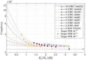
Figure 13: The decoding complexity vs. SNR for $(247,371)$ CC with its correspondinng distance-spectrum-optimal CRC codes. The CC with no CRC using soft Viterbi decoding is also given as a reference.

VI Conclusion

For a convolutionally encoded system with CRC using serial list Viterbi decoding, an optimal CC-CRC pair and the optimal list size $L$ of S-LVA should maximize the coded channel capacity of the system.

We first analyze the performance of S-LVA in great detail and prove that the expected number of decoding attempts, $\mathbb{E}[N_{\operatorname{LVA}}]$ converges to $2^{m}(1-\epsilon)$ as SNR decreases and to $1$ as SNR increases. Then we show that with SNR fixed, probability of error converges and probability of erasure tends to zero as $L$ increases up to $|\mathcal{C}|$.

Since the design of list size $L$ is independent of the design of the optimal CC-CRC pair, we deal with two design problems seperately. We first show that $L=|\mathcal{C}|$ is always the optimal list size for any candidate CC-CRC pairs. Then, with $L=|\mathcal{C}|$, since when FER is small, the corresponding coded channel capacity will be roughly the same for all candidate CC-CRC pairs, we choose the design metric of finding the optimal CC-CRC pair as the SNR gap to RCU bound proposed by Polyanskiy et al. and provides sufficient evidences showing that a weaker CC used with a stronger distance-spectrum-optimal CRC code is comparable to a single strong CC with no CRC code.

Future work will be focused on resolving the variable rate issue by considering tail-biting CC or punctured CC.

References

- [1] H. Yang, S. V. S. Ranganathan, and R. D. Wesel, “Serial list viterbi decoding with crc: Managing errors, erasures, and complexity,” in GLOBECOM 2018 - 2018 IEEE Global Communications Conference, Dec. 2018.
- [2] R. E. Blahut, Algebraic Codes for Data Transmission. Cambridge, UK: Cambridge University Press, 2003.
- [3] P. Koopman and T. Chakravarty, “Cyclic redundancy code (CRC) polynomial selection for embedded networks,” in Int. Conf. Dependable Systems and Networks, Jun. 2004, pp. 145–154.
- [4] C. Y. Lou, B. Daneshrad, and R. D. Wesel, “Convolutional-code-specific CRC code design,” IEEE Trans. Commun., vol. 63, no. 10, pp. 3459–3470, Oct. 2015.
- [5] R. Johannesson and K. S. Zigangirov, Fundamentals of Convolutional Coding, J. B. Anderson, Ed. New Jersey, USA: IEEE Press, 1999.
- [6] N. Seshadri and C. E. W. Sundberg, “List viterbi decoding algorithms with applications,” IEEE Trans. Commun., vol. 42, no. 234, pp. 313–323, Feb. 1994.
- [7] F. K. Soong and E. F. Huang, “A tree-trellis based fast search for finding the n-best sentence hypotheses in continuous speech recognition,” in Proc. Int. Conf. Acoustics, Speech, and Signal Processing (ICASSP), Apr. 1991, pp. 705–708 vol.1.
- [8] C. Nill and C. E. W. Sundberg, “List and soft symbol output viterbi algorithms: extensions and comparisons,” IEEE Trans. Commun., vol. 43, no. 2/3/4, pp. 277–287, Feb. 1995.
- [9] M. Roder and R. Hamzaoui, “Fast tree-trellis list viterbi decoding,” IEEE Trans. Commun., vol. 54, no. 3, pp. 453–461, Mar. 2006.
- [10] R. Wang, W. Zhao, and G. B. Giannakis, “CRC-assisted error correction in a convolutionally coded system,” IEEE Trans. Commun., vol. 56, no. 11, pp. 1807–1815, Nov. 2008.
- [11] M. Sybis, K. Wesolowski, K. Jayasinghe, V. Venkatasubramanian, and V. Vukadinovic, “Channel coding for ultra-reliable low-latency communication in 5g systems,” in 2016 IEEE 84th Vehicular Technology Conference (VTC-Fall), Sept 2016, pp. 1–5.
- [12] B. Chen and C. . W. Sundberg, “List viterbi algorithms for continuous transmission,” IEEE Transactions on Communications, vol. 49, no. 5, pp. 784–792, May 2001.
- [13] C. Bai, B. Mielczarek, W. A. Krzymien, and I. J. Fair, “Efficient list decoding for parallel concatenated convolutional codes,” in 2004 IEEE 15th International Symposium on Personal, Indoor and Mobile Radio Communications (IEEE Cat. No.04TH8754), vol. 4, Sept 2004, pp. 2586–2590 Vol.4.
- [14] L. Lijofi, D. Cooper, and B. Canpolat, “A reduced complexity list single-wrong-turn (swt) viterbi decoding algorithm,” in 2004 IEEE 15th International Symposium on Personal, Indoor and Mobile Radio Communications (IEEE Cat. No.04TH8754), vol. 1, Sept 2004, pp. 274–279 Vol.1.
- [15] Y. Polyanskiy, H. V. Poor, and S. Verdu, “Channel coding rate in the finite blocklength regime,” IEEE Transactions on Information Theory, vol. 56, no. 5, pp. 2307–2359, May 2010.
- [16] J. Font-Segura, G. Vazquez-Vilar, A. Martinez, A. G. i Fàbregas, and A. Lancho, “Saddlepoint approximations of lower and upper bounds to the error probability in channel coding,” in 2018 52nd Annual Conference on Information Sciences and Systems (CISS), March 2018, pp. 1–6.
- [17] S. Lin and D. J. Costello, Error Control Coding: fundamentals and applications. New Jersey, USA: Pearson Prentice Hall, 2004.