Adaptive Sparse Estimation with Side Information

Abstract

The article considers the problem of estimating a high-dimensional sparse parameter in the presence of side information that encodes the sparsity structure. We develop a general framework that involves first using an auxiliary sequence to capture the side information, and then incorporating the auxiliary sequence in inference to reduce the estimation risk. The proposed method, which carries out adaptive SURE-thresholding using side information (ASUS), is shown to have robust performance and enjoy optimality properties. We develop new theories to characterize regimes in which ASUS far outperforms competitive shrinkage estimators, and establish precise conditions under which ASUS is asymptotically optimal. Simulation studies are conducted to show that ASUS substantially improves the performance of existing methods in many settings. The methodology is applied for analysis of data from single cell virology studies and microarray time course experiments.

Keywords: Adaptive shrinkage estimation; Inference with side information; Sparsity; SURE shrinkage; Higher order minimax risk; Soft-thresholding; Two-sample inference.

1 Introduction

The recent technological advancements have made it possible to collect vast amounts of data with various types of side information such as domain knowledge, expert insights, covariates in the primary data, and secondary data from related studies. In a wide range of fields including genomics, neuroimaging and signal processing, incorporating side information promises to yield more accurate and meaningful results. However, few analytical tools are available for extracting and combining information from different data sources in high-dimensional data analysis. This article aims to develop new theory and methodology for leveraging side information to improve the efficiency in estimating a high-dimensional sparse parameter. We study the following closely related issues: (i) how to properly extract or construct an auxiliary sequence to capture useful sparsity information; (ii) how to combine the auxiliary sequence with the primary summary statistics to develop more efficient estimators; and (iii) how to assess the relevance and usefulness of the side information, as well as the robustness and optimality of the proposed method.

1.1 Motivating applications

Sparsity is an essential phenomenon that arises frequently in modern scientific studies. In a range of data-intensive application fields such as genomics and neuroimaging, only a small fraction of data contain useful signals. The detection, estimation and testing of a high-dimensional sparse object have many important applications and have been extensively studied in the literature (Donoho and Jin, 2004, Johnstone and Silverman, 2004, Abramovich et al., 2006). For instance, in the RNA-seq study that will be analyzed in Section 4.3, the goal is to estimate the true expression levels of $n=53,216$ genes for the virus strain VZV, which is the causative agent of varicella (chickenpox) and zoster (shingles) in humans (Zerboni et al., 2014). The parameter of interest (the population mean vector of gene expression) is sparse as it is known that very few genes in the generic RNA-seq kits express themselves in these single-cell virology studies (Sen et al., 2018). The accurate identification and estimation of nonzero large effects is helpful for the discovery of novel genetic biomarkers, which constitutes a key step in the development of new treatments and personalized medicine (Matsui, 2013, Holland et al., 2016, Erickson et al., 2005). Another example arises from microarray time-course (MTC) experiments that will be analyzed in Section E of the Supplementary Material. The goal is to identify genes that exhibit a specific pattern of differential expression over time. The temporal pattern, which can be revealed by estimating the differences in expression levels of genes between two time points, would help gain insights into the mechanisms of the underlying biological processes (Calvano et al., 2005, Sun and Wei, 2011). After baseline removal, the parameter of interest is the difference between two mean vectors that are both individually sparse.

In practice, the intrinsic sparsity structure of the high-dimensional parameter is often captured by side information, which can be obtained as either summary statistics from secondary data sources or can be constructed as a covariate sequence from the original data. For instance, in the RNA-seq data, expression levels corresponding to other four experimental conditions (C1, C2, C3 and C4) are also available for the same $n$ genes through related studies conducted in the lab. The heat map in Figure 1 shows that the sparse structure of the mean transcription levels of the genes for VZV is roughly maintained by the same set of genes in subjects from the other four conditions. The common structural information shared by both cases (VZV) and controls (C1 to C4) can be exploited to construct more efficient estimation procedures. In the two-sample sparse estimation problem considered in the MTC study (analyzed in Section E of the Supplementary Material), we illustrate that a covariate sequence can be constructed from the original data matrix to assist inference by capturing the sparseness of the mean difference. Intuitively, incorporating side information promises to improve the efficiency of existing methods and interpretability of results. However, in conventional practice, such useful auxiliary data have been largely ignored in analysis.

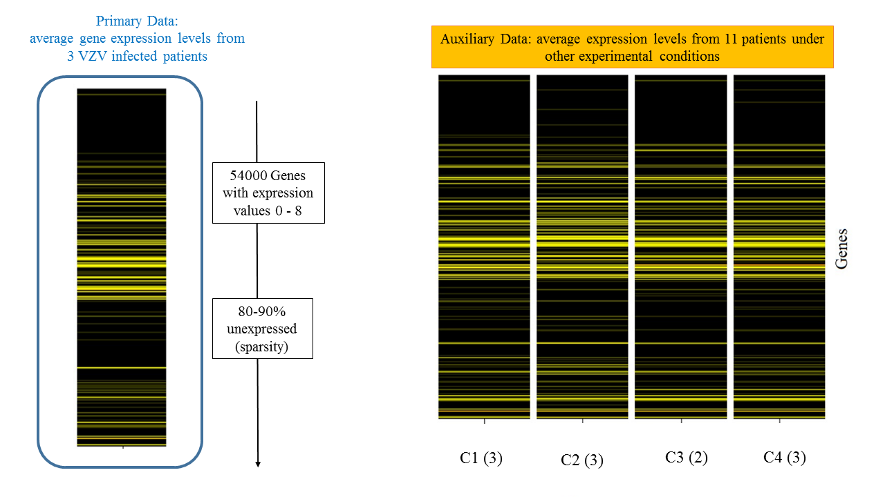
Figure 1: Heat map showing the average expression levels in the RNA-seq study. Left panel: VZV; right panel from top to bottom: C1, C2, C3 and C4, where the number of replicates (patients) is shown in parenthesis. We can see that 80-90% of the genes under the VZV condition are unexpressed (black), and the same sparse structure seems to be roughly maintained in the other four experimental conditions. Useful side information on sparsity can be extracted from secondary data (C1-C4) and be combined with the primary data (VZV) to construct more efficient estimators.

1.2 ASUS: a general framework for leveraging side information

In this article, we develop a general integrative framework for sparse estimation that is capable of handling side information that may be extracted from (i) prior or domain-specific knowledge, (ii) covariate sequence based on the same (original) data, or (iii) summary statistics based on secondary data sources. Let $\bm{\theta}=(\theta_{1},\cdots,\theta_{n})$ be an unknown high-dimensional sparse parameter. Our study focuses on the class of non-linear thresholding estimators [See Chs 8, 13 of Johnstone (2015) and Ch 11 of Mallat (2008)], which have been widely used in the sparse case where many coordinates of $\bm{\theta}$ are small or zero.

The proposed estimation framework involves two steps: first constructing an auxiliary sequence $\bm{S}=(S_{i}:1\leq i\leq n)$ to capture the sparse structure, and second combining $\bm{S}$ with the primary statistics, denoted $\boldsymbol{Y}=(Y_{i}:1\leq i\leq n)$, via a group-wise adaptive thresholding algorithm. Our idea is that the coordinates of $\boldsymbol{\theta}$ become nonexchangeable in light of side information. To reflect this heterogeneity, we divide all coordinates into $K$ groups based on $S_{i}$. The side information is then incorporated in our estimation procedure by applying soft-thresholding estimators separately, thereby fine tuning the group-wise thresholds to capture the varied sparsity levels across groups. The optimal grouping and thresholds are chosen adaptively via a data-driven approach, which employs the Stein’s unbiased risk estimate (SURE) criterion to minimize the total estimation risk. The proposed method, which carries out adaptive SURE-thresholding using side information (ASUS), is shown to have robust performance and enjoy optimality properties. ASUS is simple and intuitive, but nevertheless provides a general framework for information pooling in sparse estimation problems. Concretely, since ASUS does not rely on any functional relationships between $\bm{S}$ and $\bm{\theta}$, it is robust and effective in leveraging side information in a wide range of scenarios. In Section 2.2, we demonstrate that this flexible framework can be applied to various sparse estimation problems.

The amount of efficiency gain of ASUS depends on two factors: (i) the usefulness of the side information; and (ii) the effectiveness in utilizing the side information. To understand the first issue, we formulate in Section 3 a hierarchical model to assess the informativeness of an auxiliary sequence. Our theoretical analysis characterizes the conditions under which methods ignoring side information are suboptimal compared to an “oracle” with perfect knowledge on sparsity structure. To investigate the second issue, Section 3 establishes precise conditions under which ASUS is asymptotically optimal, in the sense that its maximal risk is close to the theoretical limit that is attained by the oracle. Finally, we carry out a theoretical analysis on the robustness of ASUS; our results show that pooling non-informative side information would not harm the performance of data combination procedures. Our asymptotic results are built upon the elegant higher-order minimax risk evaluations developed by Johnstone (1994).

1.3 Connections with existing work and our contributions

ASUS is a non-linear shrinkage estimator that incorporates relevant side information by choosing data-adaptive thresholds to reflect the varied sparsity levels across groups. We use the SURE criterion for simultaneous tuning of the grouping and shrinkage parameters. Our methodology is related to Xie et al. (2012), Tan et al. (2015) and Weinstein et al. (2018), which utilized SURE to devise algorithms reflecting optimal shrinkage directions. However, these works are developed for different purposes (addressing the heteroscedasticity issue in the data) and do not cover the sparse case.

The notion of side information in estimation has been explored in several research fields. In information theory for instance, sparse source coding with side information is a well studied problem (Wyner, 1975; Cover and Thomas, 2012; Watanabe et al., 2015). However, these methodologies focus on very different goals and cannot be directly applied to our problem. In the statistical literature, the use of side information in sparse estimation problems has been mainly limited to regression settings where the side information must be in the form of a linear function of $\bm{\theta}$ (Ke et al., 2014, Kou and Yang, 2015). By contrast, our estimation framework utilizes a more flexible scheme that does not require the specification of any functional relationship between $\bm{\theta}$ and the side information. The proposed ASUS algorithm is simple and intuitive but nevertheless enjoys strong numerical and theoretical properties. Our simulation studies show that it can substantially outperform competitive methods in many settings. ASUS is a robust data combination procedure in the sense that asymptotically it would not under-perform methods ignoring side information when the auxiliary data are non-informative (see Theorem 4).

The proposed research makes several new theoretical contributions. First, we develop general principles for constructing and pooling the side information, which guarantees proper information extraction and robust performance of ASUS. Second, we formulate a theoretical framework to assess the usefulness of side information. Third, we establish precise conditions under which ASUS is asymptotically optimal. Finally, we extend the sparse minimax decision theory of Johnstone (2015), which provides the foundation for a range of sparse inference problems (Abramovich et al., 2006, 2007, Cai et al., 2014, Tibshirani et al., 2014, Collier et al., 2017), to derive new high-order characterizations of the maximal risk of soft-thresholding estimators.

1.4 Organization of the paper

Section 2 describes the proposed ASUS procedure. Section 3 presents theoretical analyses. The numerical performances of ASUS are investigated using both simulated and real data in Section 4. Section 5 concludes with a discussion. Additional numerical results and proofs are given in the Supplementary materials.

2 Adaptive Sparse Estimation with Side Information

This section first describes the model and assumptions (Section 2.1), then discusses how to construct the auxiliary sequence (Section 2.2), and finally proposes the methodology (Section 2.3).

2.1 Model and assumptions

To conduct a systematic study of the influence of side information for estimating $\bm{\theta}$, we consider a hierarchical model that relates the primary and auxiliary data sets through a latent vector $\bm{\xi}=(\xi_{1},\ldots,\xi_{n})$, which represents the noiseless side information that encodes the sparsity information of $\bm{\theta}$. The latent vector $\bm{\xi}$ cannot be observed directly but may be partially revealed by an auxiliary sequence (noisy side information) $\bm{S}=({S}_{1},\cdots,{S}_{n})$. For instance, in the RNA-seq example, the parameter of interest is the population mean of the gene expression levels for diseased patients, and the latent variable $\xi_{i}$ may represent the quantitative outcome of a complex gene regulation process that determines whether gene $i$ expresses itself under the influence of a certain experimental condition. The primary and secondary data respectively correspond to gene expression levels for the patients from the concerned (i.e. VZV infected) and other related groups. The primary and auxiliary statistics $Y_{i}$ and $S_{i}$ for gene $i$ can be constructed based on the corresponding sample means.

For $n$ parallel units, the summary statistic $Y_{i}$ for the $i$th unit is modeled by

$$Y_{i}=\theta_{i}+\epsilon_{i},\quad\epsilon_{i}\sim N(0,\sigma_{i}^{2}),$$ (1)

where, by convention, $\sigma_{i}^{2}$ are assumed to be known or can be well estimated from data (e.g. (Brown and Greenshtein, 2009, Xie et al., 2012, Weinstein et al., 2018)). We further assume that both $\bm{\theta}$ and $\bm{S}$ are related to the latent vector $\bm{\xi}$ through some unknown real-valued functions $h_{\theta}$ and $h_{s}$:

$$\theta_{i} = h_{\theta}(\xi_{i},\eta_{1i}),$$ (2)

$$S_{i} = h_{s}(\xi_{i},\eta_{2i}),$$ (3)

where $\eta_{1i}$ and $\eta_{2i}$ follow some unspecified priors, and represent independent random perturbations that are independent of $\xi_{i}$; concrete examples for Models 1 to 3 are discussed in Section 2.2.

Remark 1.

The above model can be conceptualized as a Bayesian hierarchical model:

$$Y_{i}|(\theta_{i},S_{i})\sim N(\theta_{i},\sigma_{i}^{2}),\quad(\theta_{i},S_{i})|\xi_{i}\sim f_{1}(\theta|\xi_{i})f_{2}(s|\xi_{i}),\quad\xi_{i}\stackrel{{\scriptstyle iid}}{{\sim}}f_{3}(\xi),$$

where $f_{1},f_{2},f_{3}$ are unknown densities. In Equations 2 and 3, $\xi_{i}$ is a random quantity and independent of $\eta_{1i}$ and $\eta_{2i}$. As a special case of Equation 2, we can write $\theta_{i}=h_{\theta}(\xi_{i})$ without the random perturbations $\eta_{1i}$. Our theory is mainly stated in terms of random $\xi_{i}$’s for ease of presentation. However, we note that our theoretical results still hold even when $\xi_{i}$ is deterministic because the theory in Section 2.3 is derived conditional on $\xi_{i}$, and the proof in Section 3 is built upon an empirical density function (10).

The hierarchical Models 1 to 3 provide a general and flexible framework for our methodological and theoretical developments. In particular, it covers a wide range of scenarios by allowing the strength of the side information to vary from completely non-informative (e.g., when $\xi_{i}$ is useless, or when $S_{i}$ and $\xi_{i}$ are independent for all $i$) to perfectly informative (e.g. when $\theta_{i}=\xi_{i}$ and $S_{i}=\xi_{i}$ for all $i$). In Section 3, the usefulness of the latent vector $\bm{\xi}$ is investigated via Equation 2, and the informativeness of the auxiliary sequence $\bm{S}$ is characterized by Equations 2 and 3.

2.2 Constructing the auxiliary sequence: principles and examples

A key step in our methodological development is to properly extract side information using an auxiliary sequence. The sequence $\boldsymbol{S}$ can be constructed from various data sources including the following three basic settings: (i) prior or domain-specific knowledge; (ii) covariates or discard data in the same primary data set; or (iii) secondary data from related studies. We stress that our estimation framework is valid for all three settings as long as $\boldsymbol{S}$ fulfills the following two fundamental principles.

The first principle is informativeness, which requires that $S_{i}$ should be chosen or constructed in a way to encode the sparse structure effectively. The second principle is conditional independence, which requires that $S_{i}$ must be conditionally independent of $Y_{i}$ given the latent variable $\xi_{i}$. The conditional independence assumption, which is implied by Models 1 to 3, ensures proper shrinkage directions and plays a key role in establishing the robustness of ASUS. Examples 1 to 4 below present specific instances of auxiliary sequences fulfilling such principles, wherein the auxiliary sequences may either be readily available from distinct but related experiments or can be carefully constructed from the same (original) data to capture important structural information that is discarded by conventional practice.

Example 1. Prioritized subset analysis (PSA, Li et al., 2008). In genome wide association studies, prior data and domain knowledge such as known gene functions or interactions may be used to construct an auxiliary sequence $\bm{S}$ that can prioritize the discovery of SNPs in certain genomic regions. Typically, the primary data set can be summarized as a vector $\bm{Y}=(Y_{1},\cdots,Y_{n})$, where $Y_{i}$ are either taken as differential allele frequencies between diseased and control groups, or z-values based on $\chi^{2}$-tests assessing the association between the allele frequency and the disease status. Let $\bm{S}=({S}_{1},\cdots,{S}_{n})\in\{-1,1\}^{n}$ be an auxiliary sequence, where $S_{i}=1$ if SNP $i$ is in the prioritized subset and $S_{i}=-1$ otherwise. $\bm{S}$ can be viewed as perturbations of the true state sequence $\bm{\xi}=(\xi_{1},\cdots,\xi_{n})$, where $\xi_{i}=1$ if SNP $i$ is associated with the disease and $\xi_{i}=-1$ otherwise. The informativeness and independence principles are fulfilled when (i) the prioritized subset contains SNPs that are more likely to hold disease susceptible variants and (ii) the perturbations of $\bm{\xi}$ are random (hence $Y_{i}$ and $S_{i}$ are conditionally independent given $\xi_{i}$). Both (i) and (ii) seem reasonable assumptions in PSA studies.

Example 2. One-sample inference. In the RNA-seq study, let the primary data be $\{Y_{i,j}:i=1,\cdots,n;j=1,\cdots,k_{y}\}$ that record the expression levels of $n$ genes from $k_{y}$ subjects infected by VZV. The primary statistics are $\bm{Y}=(\bar{Y}_{1},\cdots,\bar{Y}_{n})$, where $\bar{Y}_{i}=k_{y}^{-1}\sum_{j=1}^{k_{y}}Y_{i,j}$. Let the secondary data be $\{X_{i,j}:i=1,\cdots,n;j=1,\cdots,k_{x}\}$ that record the expression levels of the same $n$ genes for $k_{x}$ subjects but under different Conditions C1 to C4. The auxiliary sequence can be constructed as $\bm{S}=({S}_{1},\cdots,{S}_{n})=(|\bar{X}_{1}|,\cdots,|\bar{X}_{n}|)$, where $\bar{X}_{i}=k_{x}^{-1}\sum_{j=1}^{k_{x}}X_{i,j}$. Thus although we record the expression levels of the same set of $n$ genes, in the case of the primary data the genes are infected with the VZV virus whereas for the secondary data the expression levels are recorded under the influence of agents that are different from that of the VZV virus. The latent state $\xi_{i}$ represents whether gene $i$ expresses itself under any of the conditions. Now we check whether the two information extraction principles are fulfilled. First, the informativeness principle holds since, as demonstrated by the heat map in Figure 1, inactive genes under VZV are likely to remain inactive under the other conditions. The sparse structure is captured by the auxiliary sequence, where a small $S_{i}$ signifies an inactive gene. Second, Section 2.1 has explained how the RNA-seq data may be sensibly conceptualized via Models (1) to (3), where $\bar{Y}_{i}$ and $S_{i}$ are conditionally independent given the latent variable $\xi_{i}$, fulfilling the second principle.

Example 3. Two-sample inference. Consider the MTC study discussed in the introduction (and analyzed in Section E of the Supplementary Material). Let $\{Y_{i,j,t_{d}}:i=1,\ldots,n;j=1,\ldots,k_{i};d=0,1,2\}$ record the expression levels of $n$ genes from $k_{i}$ subjects at time points $t_{0}$ (baseline), $t_{1}$ and $t_{2}$. Let $\bar{Y}_{i,d}=k_{i}^{-1}\sum_{j=1}^{k_{i}}(Y_{i,j,t_{d}}-Y_{i,j,t_{0}})$ be the average expression levels of gene $i$ at time point $t_{d}$ after baseline adjustment, $d=1,2$. Denote $\mu_{i,d}=E(\bar{Y}_{i,d})$ and $\boldsymbol{\mu}_{d}=(\mu_{i,d}:1\leq i\leq n)$. Then both $\boldsymbol{\mu}_{1}$ and $\boldsymbol{\mu}_{2}$ are individually sparse. The parameter of interest is $\theta_{i}=\mu_{i,1}-\mu_{i,2}$, which can be estimated by the primary statistic ${Y}_{i}=\bar{Y}_{i,1}-\bar{Y}_{i,2}$. Denote the union support $\mathcal{U}=\{i:\mu_{i,1}\neq 0\;\mbox{or}\;\mu_{i,2}\neq 0\}$. Then $\mathcal{U}$ can be exploited to screen out zero effects since if $i\notin\mathcal{U}$, we must have $\theta_{i}=0$. Consider the sequence $S_{i}=|\bar{Y}_{i,1}+\kappa_{i}\bar{Y}_{i,2}|$, where $\kappa_{i}=\hat{\sigma}_{i,1}/\hat{\sigma}_{i,2}$ and $\hat{\sigma}_{i,d}^{2}=(k_{i}-1)^{-1}\sum_{j=1}^{k_{i}}(Y_{i,j,t_{d}}-Y_{i,j,t_{0}}-\bar{Y}_{i,d})^{2}$. Then the auxiliary sequence is informative since a large $S_{i}$ provides strong evidence that $i\in\mathcal{U}$. The union support encodes the sparse structure of $\boldsymbol{\theta}$. Moreover, $Y_{i}$ and $S_{i}$ are asymptotically independent with our choice of $\kappa_{i}$ (Proposition 6 in Cai et al., 2018). Hence both principles are fulfilled.

Example 4. Estimation under the ANOVA setting. This example is an extension of Example 3 to multi-sample inference. Consider $m$ conditions $d=1,\ldots,m$, $m\geq 2$. The parameter of interest is $\bm{\theta}_{n\times 1}=\Gamma\mathbf{a}$, where $\Gamma_{n\times m}=(\bm{\mu}_{1},\dots,\bm{\mu}_{m})$, $\mu_{i,d}=\mathbb{E}(\bar{Y}_{i,d})$ and $\mathbf{a}_{m\times 1}$ is a vector of known weights. Here $\bm{\theta}$ may represent a weighted average of true transcription levels of $n$ genes across $m$ time points. Let $\mathbf{D}_{i}=(\bar{Y}_{i,1},\ldots,\bar{Y}_{i,m})$ be the vector of average expression level of gene $i$ for the $m$ time points after baseline adjustment and denote $\mathbb{D}_{n\times m}=(\mathbf{D}_{1},\ldots,\mathbf{D}_{n})^{T}$. To estimate $\bm{\theta}$, our proposed framework suggests using the usual unbiased estimator $\boldsymbol{Y}=\mathbb{D}\mathbf{a}$ as the primary statistic, and $\boldsymbol{S}=\mathbb{D}\mathbf{b}$ as the auxiliary sequence for some weights $\mathbf{b}$. The informativeness principle from Example 3 continues to hold under this setting. To fulfil the independence principle, we choose $\mathbf{b}$ such that ${Cov}(\boldsymbol{Y},\bm{S})=\mathbf{0}$.

In Examples 3 and 4, the auxiliary sequence $\bm{S}$ is constructed from the same original data matrix. We give some intuitions to explain why $\bm{S}$ is useful. The conventional practice reduces the original data into a vector of summary statistics $\bm{Y}$. However, this data reduction step often causes significant loss of information and thus leads to suboptimal procedures. Specifically, the information on the sparseness of the union support $\mathcal{U}$ is lost in the data reduction step. The key idea in Example 3 is that the auxiliary sequence $\boldsymbol{S}$ captures the structural information on sparsity, which is discarded by conventional practice. Therefore by incorporating $\boldsymbol{S}$ into the inferential process we can improve the efficiency of existing methods. Note that $\bm{Y}$ is not a sufficient statistic for estimating $\boldsymbol{\theta}$, the minimax estimation error based on $(\bm{Y},\bm{S})$ can greatly improve the performance of all estimators that are based on $\bm{Y}$ alone; a rigorous theoretical analysis is carried out in the proof of Theorem 2. To summarize, the above examples illustrate that the side information can be either “external” (Examples 1-2) or “internal” (Examples 3-4). The key in the proposed estimation framework, which we discuss next, is to construct a proper auxiliary sequence that fulfills the two fundamental principles. We shall develop a unified estimation framework that is capable of handling both internal and external side information.

We conclude this section with two remarks. First, the conditional independence assumption can be relaxed; the methodology would work as long as $Y_{i}$ and $S_{i}$ are conditionally uncorrelated (c.f. Proposition 1). Second, we do not require $Y_{i}$ or $\theta_{i}$ to be related to $S_{i}$ through any functional forms; hence classical regression techniques (even nonparametric models) cannot be applied in the above scenarios. We aim to develop a general information pooling strategy that does not involve any prescribed functional relationships; a methodology in this spirit is described next.

2.3 The ASUS estimator and its risk properties

Let $\boldsymbol{Y}$ and $\bm{S}$ denote the primary statistics and auxiliary sequence obeying Models (1) to (3). Let $\eta_{t}(.)$ be a soft-thresholding operator such that

$$\eta_{t}(Y_{i})=\begin{cases}-Y_{i}\sigma^{-1}_{i}\text{, if }|Y_{i}\sigma^{-1}_{i}|\leq t;\\ -t\text{ sign}(Y_{i}\sigma^{-1}_{i})\text{, otherwise}.\end{cases}$$

The proposed ASUS estimator operates in two steps: first constructing $K$ groups using $\bm{S}$, and second applying soft-thresholding within each group using $\bm{Y}$. The construction of the groups relies only on $\bm{S}$. The tuning parameters for both grouping and shrinkage are determined using the SURE criterion.

Procedure 1.

For $k=1,\ldots,K$ and $\bm{\tau}=\{\tau_{1}<\ldots<\tau_{K-1}\}$, denote $\widehat{\mathcal{I}}_{k}^{\tau}=\{i:\tau_{k-1}<S_{i}\leq\tau_{k}\}$ with $\tau_{0}=-\infty$, $\tau_{K}=\infty$. Consider the following class of shrinkage estimators:

$$\hat{\theta}^{SI}_{i}(\mathcal{T})\coloneqq Y_{i}+\sigma_{i}\eta_{t_{k}}(Y_{i})\text{ if }i\in\widehat{\mathcal{I}}_{k}^{\tau},$$ (4)

where, $\mathcal{T}=\{\tau_{1},\dots,\tau_{K-1},~{}t_{1},\ldots,t_{K}\}$ and each of the threshold hyper-parameters $t_{1},\ldots,t_{K}$ varies in $[0,t_{n}]$ with $t_{n}=(2\log n)^{1/2}$. Thus, the set of all possible hyper-parameter $\mathcal{T}$ values is $\mathcal{H}_{n}=\mathbf{R}^{K-1}_{+}\times[0,t_{n}]^{K}$. Define the SURE function

$$S(\mathcal{T},\boldsymbol{Y},\bm{S})=n^{-1}\left[\sum_{i=1}^{n}\sigma^{2}_{i}+\sum_{k=1}^{K}\sum_{i\in\widehat{\mathcal{I}}_{k}^{\tau}}\left\{\sigma^{2}_{i}(|Y_{i}\sigma_{i}^{-1}|\wedge t_{k})^{2}-2\sigma^{2}_{i}\,I(|Y_{i}\sigma_{i}^{-1}|\leq t_{k})\right\}\right].$$ (5)

Let $\hat{\mathcal{T}}=\operatorname*{arg\,min}_{\mathcal{T}\in\mathcal{H}_{n}}\,S(\mathcal{T},\boldsymbol{Y},\bm{S})$. Then, the ASUS estimator is given by $\hat{\theta}^{SI}_{i}(\hat{\mathcal{T}})$.

Remark 2.

When $\bm{\theta}$ is very sparse, the empirical fluctuations in the SURE function would have non-negligible effects on thresholding procedures. We suggest choosing $t_{1},\ldots,t_{k}$ for a given grouping by implementing a hybrid scheme that is similar to the SureShrink estimator of Donoho and Johnstone (1995), e.g. setting $t_{k}=t_{n}$ if $|\widehat{\mathcal{I}}_{k}^{\tau}|^{-1}\sum_{i\in\widehat{\mathcal{I}}_{k}^{\tau}}(Y_{i}^{2}/\sigma_{i}^{2})\wedge t_{n}^{2}-1\leq n^{-1/2}\log^{3/2}n$.

We present a toy example to illustrate why ASUS works. Consider the two-sample inference problem described by Example 3 in Section 2.2. Let $\theta_{i}=\mu_{i,1}-\mu_{i,2}$ and $\bar{Y}_{i,d}\sim N(\mu_{i,d},0.25)$, where $d=1,2$, $i=1,\ldots,n$, and $n=10^{4}$. For $\bm{\mu}_{1}$ we generate the first $20\%$ of its coordinates randomly from $\mbox{Unif}(4,6)$, the next $20\%$ randomly from $\mbox{Unif}(2,3)$ and set the remaining coordinates to $0$. For $\bm{\mu}_{2}$, the first $20\%$ are from $\mbox{Unif}(1,2)$, the next $20\%$ from $\mbox{Unif}(1,6)$ and the remaining $0$. Finally, we let $\bar{Y}_{i}=\bar{Y}_{i,1}-\bar{Y}_{i,2}$ and $S_{i}=|\bar{Y}_{i,1}+\bar{Y}_{i,2}|$. The left panel in Figure 2 presents the histogram of $\boldsymbol{Y}=(\bar{Y}_{i}:1\leq i\leq n)$, where the lighter shade corresponds to $\bar{Y}_{i}$ with $\theta_{i}=0$. The SureShrink estimator in Donoho and Johnstone (1995) chooses threshold $t=0.6$ for all observations, resulting in an MSE of 0.338. Imagine that an oracle has the perfect knowledge about the two groups ($\theta_{i}=0$ vs. $\theta_{i}\neq 0$). In group 0, SureShrink chooses $t_{0}=4.2$, whereas in group 1, SureShrink chooses $t_{0}=0.15$. The total MSE is reduced to 0.20 by adopting varied thresholds for the two groups. In practice, the groups cannot be identified perfectly but can be partially revealed by the auxiliary statistic $S_{i}=|\bar{Y}_{i,1}+\bar{Y}_{i,2}|$, where a small $S_{i}$ signifies a possible zero effect. Our simulation studies in Section 4 show that by exploiting the side information in $S_{i}$, ASUS achieves substantial gain in performance over conventional methods.

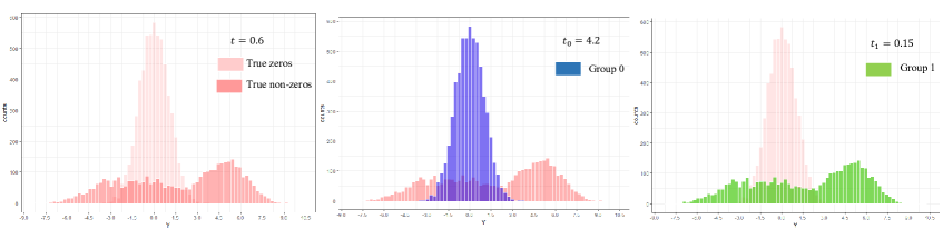
Figure 2: Toy example depicting ASUS. Left: SureShrink estimator at $t=0.6$. Middle: ASUS with group 0 and $t_{0}=4.2$. Right: ASUS with group 1 and $t_{1}=0.15$.

Let $l_{n}(\bm{\theta},\bm{\widehat{\theta}})=n^{-1}\|\bm{\widehat{\theta}}-\bm{\theta}\|^{2}_{2}$ denote the squared error loss of estimating $\bm{\theta}$ using $\widehat{\bm{\theta}}$. For each member $\hat{\bm{\theta}}^{SI}(\mathcal{T})$ in our class of estimators, $\mathcal{T}\in\mathcal{H}_{n}$, denote its risk by $r_{n}(\mathcal{T};\bm{\theta})=\mathbb{E}\left[l_{n}\left\{\bm{\theta},\hat{\bm{\theta}}^{SI}(\mathcal{T})\right\}\right]$, where the expectation is taken with respect to the joint distribution of $(Y_{i},S_{i})$. The next proposition shows that (5) provides an unbiased estimate of the true risk.

Proposition 1.

Consider Models (1) to (3). Then given $\xi_{i}$, the pair $\bigl{\{}(Y_{i}-\theta_{i})\eta_{t_{k}}(Y_{i}),I(i\in\widehat{\mathcal{I}}_{k}^{\tau})\bigr{\}}$ are uncorrelated. It follows that $r_{n}(\mathcal{T};\bm{\theta})=\mathbb{E}\{S(\mathcal{T},\boldsymbol{Y},\bm{S})\}$.

Next we study the large-sample behavior of the proposed SURE criterion. As in Xie et al. (2012), we impose the following assumption on the fourth moment of the noise distributions:

$$\mathrm{(A1)} \varlimsup_{n\to\infty}\dfrac{1}{n}\sum_{i=1}^{n}\sigma_{i}^{4}<\infty~{}.$$

The following theorem shows that the risk estimate $S(\mathcal{T},\boldsymbol{Y},\bm{S})$ is uniformly close to the true risk as well as the loss, justifying our proposed hyper-parameter estimate $\mathcal{\hat{T}}$. Compared to Xie et al. (2012) (theorem 3.1) and Brown et al. (2017) (theorem 4.1), we obtain explicit rates of convergence by tracking the empirical fluctuations in the SURE function through sharper concentration inequalities.

Theorem 1.

Under Assumption A1, with $c_{n}=n^{1/2}(\log n)^{-\delta}$ for any $\delta>3/2$, we have

$$\textrm{(a)}\quad\lim_{n\to\infty}\;\;c_{n}\;\;\mathbb{E}\Big{\{}\sup_{\mathcal{T}\in\mathcal{H}_{n}}\Big{|}S(\mathcal{T},\boldsymbol{Y},\bm{S})-r_{n}(\mathcal{T};\bm{\theta})\Big{|}\Big{\}}=0,$$

$$\textrm{(b)}\quad\lim_{n\to\infty}\;\;c_{n}\;\mathbb{E}\Big{[}\sup_{\mathcal{T}\in\mathcal{H}_{n}}\Big{|}S(\mathcal{T},\boldsymbol{Y},\bm{S})-l_{n}\{\bm{\theta},\hat{\bm{\theta}}^{SI}(\mathcal{T})\}\Big{|}\Big{]}=0,$$

where the expectation is with respect to the joint distribution of $\boldsymbol{Y},\bm{S}$.

Define $\mathcal{T}^{OL}$ as the minimizer of the true loss function: $\mathcal{T}^{OL}=\operatorname*{arg\,min}_{\mathcal{T}\in\mathcal{H}_{n}}l_{n}\{\bm{\theta},\bm{\hat{\theta}}^{SI}(\mathcal{T})\}$. $\mathcal{T}^{OL}$ is referred to as the oracle loss hyper-parameter as it involves the knowledge of of $\bm{\theta}$. It provides the theoretical limit that one can reach if allowed to minimize the true loss. Let $\bm{\hat{\theta}}^{SI}(\mathcal{T}^{OL})$ be the corresponding oracle loss estimator. The following corollary establishes the asymptotic optimality of $\hat{\mathcal{T}}$.

Corollary 1.

Under assumption A1, if $\lim_{n\to\infty}c_{n}\,{n^{-1/2}}\log^{\delta}n=0$ for any $\delta>3/2$, then
(a) The loss of $\bm{\hat{\theta}}^{SI}(\hat{\mathcal{T}})$ converges in probability to the loss of $\bm{\hat{\theta}}^{SI}(\mathcal{T}^{OL})$:

$$\lim_{n\to\infty}\mathbb{P}\left[l_{n}\left\{\bm{\theta},\bm{\hat{\theta}}^{SI}(\hat{\mathcal{T}})\right\}\geq l_{n}\left\{\bm{\theta},\bm{\hat{\theta}}^{SI}(\mathcal{T}^{OL})\right\}+c_{n}^{-1}\epsilon\right]=0\text{ for any }\epsilon>0~{}.$$

(b) The risk of $\bm{\hat{\theta}}^{SI}(\hat{\mathcal{T}})$ converges to the risk of the oracle loss estimator:

$$\lim_{n\to\infty}c_{n}\;\mathbb{E}\left[l_{n}\left\{\bm{\theta},\bm{\hat{\theta}}^{SI}(\hat{\mathcal{T}})\right\}-l_{n}\left\{\bm{\theta},\bm{\hat{\theta}}^{SI}(\mathcal{T}^{OL})\right\}\right]=0~{}.$$

2.4 Approximating the Bayes rule by ASUS

This section discusses a Bayes setup and illustrates how ASUS may be conceptualized as an approximation to the Bayes oracle estimator.

Consider a hierarchical model where $\theta_{i}$ has an unspecified prior and $Y_{i}\stackrel{{\scriptstyle ind.}}{{\sim}}N(\theta_{i},\sigma^{2}_{i})$ with $\sigma_{i}^{2}$ known. In the absence of any auxiliary sequence $\bm{S}$ and when $\sigma_{i}$ are all equal to, say $\sigma$, the optimal estimator is

$$\delta_{i}^{\pi}=E(\theta_{i}|y_{i})=y_{i}+\sigma^{2}\frac{f^{\prime}(y_{i})}{f(y_{i})},$$ (6)

which is known as Tweedie’s formula (Efron, 2011). When the marginal densities $f(y_{i})$ are unknown, (6) can be implemented in an empirical Bayes (EB) framework. For example, Brown and Greenshtein (2009) used kernel methods to estimate unknown densities and showed that the resulting EB estimator is asymptotically optimal under mild conditions. Under the sparse setting, an effective approach to incorporate the sparsity structure is to consider, for example, spike-and-slab priors (Johnstone and Silverman, 2004). In decision theory it has been established that the posterior median is minimax optimal under spike-and-slab priors; see Thoerem 1 of Johnstone and Silverman (2004). Hence the soft-threshold estimators can be viewed as good surrogates to the Bayes rule under sparsity. When the sparsity level is unknown, the threshold should be chosen adaptively using a data-driven method.

For a given pair of primary and auxiliary statistics $(Y_{i},S_{i})$, the Bayes oracle estimator is

$$\delta_{i}^{\pi}=E(\theta_{i}|Y_{i},S_{i}).$$ (7)

Conditionally on $S_{i}$, a Tweedie’s formula for equation (7) can be written which would require estimating the conditional marginal densities $f(y_{i}|s_{i})$ and its derivatives. ASUS can be viewed as a two-step approximation to the oracle estimator (7). The first step involves using the auxiliary sequence to divide the $n$ coordinates into $K$ groups: $\delta_{i}^{\pi}\approx\hat{\delta}_{k}(Y_{i})=E(\theta_{i}|Y_{i},i\in G_{k})=E(\theta_{i}|Y_{i},S_{i}^{*}=k),$ which can be viewed as a discrete approximation to the oracle rule (7) by discretizing $S_{i}$ as a categorical variable $S_{i}^{*}$ taking values $k=1,\cdots,K$. The second step involves setting thresholds for separate groups to incorporate the updated structural information from the auxiliary sequence. This step makes sense because under the sparse regime, it is natural to use the class of soft-thresholding estimators as a convenient surrogate to the Bayes rule, and ideally the threshold should be set differently to reflect the varied sparsity levels across the groups. Finally the optimal grouping and optimal thresholds are chosen by minimizing a SURE criterion.

This Bayesian interpretation reveals that ASUS may suffer from information loss in the discretization step. However, fully utilizing the auxiliary data by modeling $\bm{S}$ as a continuous variable is practically impossible under the ASUS framework since the search algorithm cannot deal with a diverging number of groups. Moreover, directly implementing (7) using bivariate Tweedie approaches is highly nontrivial and requires further research. ASUS, thus, seems to provide a simple, feasible yet effective framework to incorporate the side information.

3 Theoretical Analysis

This section studies the theoretical properties of ASUS under the important setting where $\bm{\theta}$ is sparse. By contrast, the results of Section 2.3 hold for any sequence $\bm{\theta}$. To simplify the presentation, we focus on a class of thresholding estimators that utilize two groups. The two-group model provides a natural choice for some important applications such as the prioritized subset analysis and RNA-seq study, but the proposed ASUS framework can handle more groups. The major goal of our theoretical analysis is to gain insights on sparse inference with side information, for which the simple two-group setup helps in two ways. First, it leads to a concise and intuitive characterization of the potential influence of side information on simultaneous estimation. Second, it enables us to develop precise conditions under which ASUS is asymptotically optimal.

3.1 Asymptotic set-up

Consider hierarchical Models (1) to (3). We begin by considering an oracle estimator $\tilde{\bm{\theta}}_{n}^{SI}(\mathcal{T}_{n}^{OR})$ that directly uses the noiseless side information $\bm{\xi}$:

$$\tilde{\theta}^{SI}_{i,n}(\mathcal{T}^{OR}_{n})\coloneqq\begin{cases}Y_{i}+\sigma_{i}\eta_{t_{1}^{*}}(Y_{i})\text{ if }i\in\mathcal{I}_{1,n}^{\tau^{\star}},\\ Y_{i}+\sigma_{i}\eta_{t_{2}^{*}}(Y_{i})\text{ if }i\in\mathcal{I}_{2,n}^{\tau^{\star}},\end{cases}$$ (8)

where $\mathcal{I}_{1,n}^{\tau}=\{i:\xi_{i}\leq\tau\}$, $\mathcal{I}_{2,n}^{\tau}=\{i:\xi_{i}>\tau\}$, and

$$\mathcal{T}^{OR}_{n}:=(\tau^{\star}_{n},t_{1,n}^{*},t_{2,n}^{*})=\operatorname*{arg\,min}_{\mathcal{T}\in\mathbf{R}\times[0,t_{n}]\times[0,t_{n}]}\,\mathbb{E}\,l_{n}\left\{\bm{\theta},\tilde{\bm{\theta}}^{SI}(\mathcal{T})\right\}.$$ (9)

Remark 3.

Both the oracle estimator $\tilde{\bm{\theta}}_{n}^{SI}(\mathcal{T}_{n}^{OR})$ and the oracle loss estimator $\bm{\hat{\theta}}^{SI}(\mathcal{T}^{OL})$ assume the knowledge of $\boldsymbol{\theta}$. However, they are different in that the former creates groups based on $\bm{\xi}$, whereas the latter uses $\boldsymbol{S}$. The purposes of introducing these two oracle estimators are different: $\bm{\hat{\theta}}^{SI}(\mathcal{T}^{OL})$ is used to assess the effectiveness of the SURE criterion; by contrast, $\tilde{\bm{\theta}}_{n}^{SI}(\mathcal{T}_{n}^{OR})$ is employed to evaluate the usefulness of the noiseless side information, i.e. the maximal improvement in performance that can be achieved by incorporating $\boldsymbol{\xi}$.

Denote $\pi_{1,n}=n^{-1}\sum_{i=1}^{n}\mathcal{I}(\xi_{i}\leq\tau^{\star}_{n})$ and $\pi_{2,n}=1-\pi_{1,n}$. Intuitively, the optimal partition $\tau_{n}^{\star}$ (within the class of thresholding procedures utilizing two groups) is chosen to maximize the “discrepancy” between the two groups. For units in group $\mathcal{I}_{k,n}^{\tau^{\star}}$, the mixture density of $\theta_{i}$ is given by

$$g_{k,n}(\theta)=(1-p_{k,n})\,\delta_{0}\,+\,p_{k,n}\,{h_{k,n}}(\theta),\quad k=1,2,$$ (10)

where $\delta_{0}$ is a dirac delta function (null effects), $h_{k,n}$ is the (alternative) empirical density of non-null effects. Following remark 1, our theory developed based on the empirical density (10) can handle both random and deterministic models; this can be more clearly seen in our proofs of the theorems. Here $p_{k,n}$ is the conditional proportion of non-null effects for a given group and may be conceptualized as the probability that a randomly selected unit in group $\mathcal{I}_{k,n}^{\tau^{\star}}$ is a non-null effect.

We consider an asymptotic set-up based on the sparse estimation framework in chapter 8.6 of Johnstone (2015), which has been widely used in high-dimensional sparse inference (Johnstone and Silverman, 1997, Abramovich et al., 2006, Donoho et al., 1998, Mukherjee and Johnstone, 2015, Cai and Sun, 2017). Let $p_{1,n}=n^{-\alpha}$ and $p_{2,n}=n^{-\beta}$ for some $0<\alpha<\beta\leq 1$. Define $\rho_{n}=\pi^{-1}_{1,n}\pi_{2,n}$. Consider the following parameter space

$${\Theta_{n}(\alpha,\beta,\rho_{n})}=\big{\{}\bm{\theta}\in\mathbb{R}^{n}:\left\lVert\bm{\theta}\right\rVert_{0}\leq{n(n^{-\alpha}+\rho_{n}n^{-\beta})}/{(1+\rho_{n})}\big{\}}.$$

The maximal risk of ASUS over $\Theta_{n}(\alpha,\beta,\rho_{n})$ is

$$\mathcal{R}^{AS}_{n}(\alpha,\beta,\rho_{n})=\sup_{{\bm{\theta}}\in\Theta_{n}(\alpha,\beta,\rho_{n})}r_{n}(\mathcal{\hat{T}},{\bm{\theta}}).$$

Correspondingly, over the same parameter space $\Theta_{n}(\alpha,\beta,\rho_{n})$, we let $\mathcal{R}^{OS}_{n}(\alpha,\beta,\rho_{n})$ denote the maximal risk of the oracle procedure $\tilde{\bm{\theta}}^{SI}_{n}(\mathcal{T}^{OR}_{n})$, and $\mathcal{R}^{NS}_{n}(\alpha,\beta,\rho_{n})$ the minimax risk of all soft thresholding estimators without side information.

The risk difference $\mathcal{R}^{NS}_{n}-\mathcal{R}^{OS}_{n}$ is a key quantity that will be used in later analysis as the benchmark decision theoretic improvement due to incorporation of side information. Specifically, the noiseless side information $\boldsymbol{\xi}$ is useful if it provides non-negligible improvement on the risk:

$$\lim_{n\to\infty}n(\mathcal{R}^{NS}_{n}-\mathcal{R}^{OS}_{n})=\infty.$$ (11)

Moreover, the ASUS estimator is asymptotically optimal if its risk improvement over $\mathcal{R}^{NS}_{n}(\alpha,\beta,\rho_{n})$ is asymptotically equal to that of the oracle:

$$\mathcal{RI}_{n}=\frac{\mathcal{R}_{n}^{NS}-\mathcal{R}_{n}^{AS}}{\mathcal{R}_{n}^{NS}-\mathcal{R}_{n}^{OS}}\rightarrow 1\mbox{ as $n\rightarrow\infty$}.$$ (12)

3.2 Usefulness of side information

We focus on Model (10), a hypothetical model based on the oracle partition $\tau_{n}^{\star}$. We state a few conditions that are needed in later analysis; some are essential for characterizing the situations where the side information is useful, i.e. the oracle estimator $\tilde{\bm{\theta}}_{n}^{SI}(\mathcal{T}_{n}^{OR})$ would provide non-negligible efficiency gain over competitive estimators.

(A2.1) $\lim_{n\to\infty}\rho_{n}\,n^{-\gamma_{0}}=0$ for some $\gamma_{0}<\beta-\alpha$.

(A2.2) For some $\nu<1/2$ and $k_{n}=\log n$, $\lim_{n\to\infty}k_{n}^{\nu}(1-\pi_{1,n})=\infty$.

(A2.3) For some $\nu<1/2$, $\lim_{n\to\infty}n^{\nu}\,\pi_{1,n}p_{1,n}\ =\infty$.

(A2.4) Let $\bar{\sigma^{2}_{n}}=n^{-1}\sum_{i=1}^{n}\sigma_{i}^{2}$ and $0<\varliminf_{n\to\infty}\bar{\sigma^{2}_{n}}\leq\varlimsup_{n\to\infty}\bar{\sigma^{2}_{n}}<\infty$.

Remark 4.

(A2.1) implies $\pi_{2,n}\,p_{2,n}/(\pi_{1,n}\,p_{1,n})\to 0$, which ensures that the oracle partition is effective in the sense that the two resulting groups have different sparsity levels. The asymmetric condition can be easily flipped for generalization. (A2.2) is a mild condition which allows $\pi_{1,n}$ to approach $1$ but at a controlled rate. (A2.3) prevents the trivial setting where ASUS reduces to the SureShrink procedure with universal threshold $\sqrt{2\log n}$, i.e. the side information would not have any influence in the estimation process. See lemma 3 (section B supplementary material) which shows that if $\varlimsup_{n\to\infty}~{}n^{1/2}\pi_{1,n}p_{1,n}<\infty$, then ASUS reduces to the SureShrink procedure, i.e. there is no need for creating groups. (A2.4) is a mild condition that is satisfied in most real life applications.

Now we study the usefulness of the noiseless side information. Following the theory in Johnstone (1994), the next theorem explicitly evaluates the risk difference $\mathcal{R}^{NS}_{n}-\mathcal{R}^{OS}_{n}$ up to higher order terms. The analysis overcomes the crudeness of the first order asymptotics for evaluating thresholding rules as pointed out by Bickel (1983) and Johnstone (1994).

Theorem 2.

Consider the oracle estimator defined in (8)-(9). Under assumption A2.1, with $k_{n}=\log n$, for all $\nu<1$, we have,

$$\mathcal{R}^{NS}_{n}(\alpha,\beta,\rho_{n})-\mathcal{R}^{OS}_{n}(\alpha,\beta,\rho_{n})=\pi_{1,n}\,p_{1,n}\,\bar{\sigma^{2}_{n}}\left\{\log\pi_{1,n}^{-1}(2-3\alpha^{-1}k_{n}^{-1})+O(k_{n}^{-\nu})\right\}.$$

It follows from (A2.3) that $\lim_{n\to\infty}n(\mathcal{R}^{NS}_{n}-\mathcal{R}^{OS}_{n})=\infty$, establishing (11).

3.3 Asymptotic optimality of ASUS

To evaluate the efficiency of ASUS, we need to compare the segmentation used by ASUS with that used by the oracle estimator. For a given segmentation hyper-parameter $\tau$, define

$$\tilde{q}^{jk}_{i,n}(\tau)\coloneqq\mathbb{P}_{n}(\hat{I}_{i}^{j}|I_{i}^{k}\Big{)}\text{ for }j,k\in\{1,2\},\;i=1,\ldots,n,$$

where $\hat{I}_{i}^{1}=\{S_{i}\leq{\tau}\}$, $I_{i}^{1}=\{\xi_{i}\leq\tau^{\star}_{n}\}$, $\hat{I}_{i}^{2}=\mathbf{R}\setminus\hat{I}_{i}^{1}$, ${\text{I}}_{i}^{2}=\mathbf{R}\setminus I_{i}^{1}$, and the probability operator $\mathbb{P}_{n}$ is based on Model (10). Let

$$q^{jk}_{i,n}(\tau)=\tilde{q}^{jk}_{i,n}(\tau)\quad\text{ if }\inf_{\tau\in\mathbf{R}}\pi_{2,n}\tilde{q}_{n}^{12}(\tau)+\pi_{1,n}\tilde{q}_{n}^{21}(\tau)<\inf_{\tau\in\mathbf{R}}\pi_{1,n}\tilde{q}_{n}^{11}(\tau)+\pi_{2,n}\tilde{q}_{n}^{22}(\tau)$$

and otherwise $q^{jk}_{i,n}(\tau)=\tilde{q}^{kk}_{i,n}(\tau)$ and $q^{kk}_{i,n}(\tau)=1-q^{jk}_{i,n}(\tau)$ for $j\neq k$. Denote the weighted average

$$q^{jk}_{n}(\tau)=\frac{\sum_{i=1}^{n}q^{jk}_{i,n}(\tau)\sigma_{i}^{2}}{\sum_{i=1}^{n}\sigma_{i}^{2}},\quad j,k\in\{1,2\}.$$

Viewing the data-driven grouping step of ASUS as a classification procedure with the oracle segmentation corresponding to the true states, we can conceptualize $q^{21}_{n}(\tau_{n})$ and $q^{12}_{n}(\tau_{n})$ as misclassification rates. Define the efficiency ratio

$$\mathcal{E}_{n}=\frac{\mathcal{R}_{n}^{NS}-\mathcal{R}_{n}^{OS}}{\mathcal{R}_{n}^{AS}-\mathcal{R}_{n}^{OS}}.$$ (13)

For notational simplicity, the dependence of this ratio on $\alpha,\beta,\rho_{n}$ is not explicitly marked. It follows from (12) that $\mathcal{RI}_{n}=1-\mathcal{E}_{n}^{-1}$. Hence a larger $\mathcal{E}_{n}$ signifies better performance of ASUS. In particular, $\mathcal{E}_{n}\to\infty$ implies the asymptotic optimality of ASUS. The poly-log rates in the following theorem are sharp.

Theorem 3.

Assume (A2.1) – (A2.4) hold. Let $k_{n}=\log n$. If there exists a sequence $\{\tau_{n}\}_{n\geq 1}$ such that

$$\lim_{n\to\infty}k_{n}^{2}\,q^{21}_{n}(\tau_{n})=0\text{ and }\lim_{n\to\infty}\rho_{n}\,q^{12}_{n}(\tau_{n})=0,$$ (14)

then ASUS is asymptotically optimal. In particular, for all $\nu<1$ we have

$$\varliminf_{n\to\infty}k_{n}^{-\nu}\mathcal{E}_{n}\geq\,2\varliminf_{n\to\infty}\log\pi_{1,n}^{-1}.$$ (15)

Next we present two hierarchical models, respectively with sub-Gaussian (SG) and sub-Exponential (SExp) tails, under which the misclassification rates can be adequately controlled. Let $S_{i}|\xi_{i}$ be independent random variables with $\mu_{i}:=\mu_{i}(\xi_{i})$ and $(\nu_{i}(\xi_{i}),b_{i}(\xi_{i}))$ such that $\mathbb{E}\,\{\exp(\lambda(S_{i}-\mu_{i}))\}\leq\exp(\nu_{i}^{2}\lambda^{2}/2)\text{ for all i and all }|\lambda|\leq b_{i}^{-1}.$ Let $\varlimsup_{i}b_{i}<\infty$, $\varlimsup_{i}\nu_{i}<\infty$ and $\bar{b}_{n}=\sup_{1\leq i\leq n}\max(2\nu_{i}^{2},b_{i})$. When $b_{i}=0$, the distribution of ${S}_{i}$ has sub-Gaussian tails. For two partitions $A$ and $B$ of the set $\{1,\ldots,n\}$, define the $\ell_{1}$ distance between the two sets $\{\mu_{i}:i\in A\}$ and $\{\mu_{i}:i\in B\}$ by $\textrm{dist}(A,B)=\inf\{|x-y|:x\in A,y\in B\}$. Let $c_{n}=\bar{b}_{n}(2\log k_{n}+\log\rho_{n})$. The following lemma provides a sufficient condition under which the requirements on misclassification rates (14) are satisfied. The proof of the lemma follows directly from the standard bounds for sub-Gaussian and sub-Exponential tails.

Lemma 1.

Let $I^{*}_{1,n}=\{i:\xi_{i}\leq\tau^{\star}_{n}\}$ and $I^{*}_{2,n}=\{1,\ldots,n\}\setminus I^{*}_{1,n}$. The requirements on misclassification rates given by (14) are satisfied if

$$\varliminf_{n\to\infty}c_{n}^{-\gamma}\textrm{dist}(I^{*}_{1,n},I^{*}_{2,n})>\gamma,$$

where $\gamma$ is $1/2$ if $\sup_{i}b_{i}=0$ and $1$ otherwise.

3.4 Robustness of ASUS

This section carries out a theoretical analysis to address the concern whether the performance of data combination procedures would deteriorate when pooling non-informative auxiliary data. We first characterize asymptotic regimes under which auxiliary data are non-informative (while the attention is confined to the prescribed class of two-group ASUS estimators), and then show that under such regimes, ASUS is robust in performance in the sense that it does not under-perform standard soft-thresholding methods.

Theorem 4.

Suppose (A2.1) – (A2.4) hold. Let $\rho_{n}=n^{\gamma_{0}}$ and $k_{n}=\log n$.

(a) Consider the following situations: (i) $\lim_{n\to\infty}k_{n}^{-1}\rho_{n}q^{21}_{n}(\tau_{n})=\infty$; and (ii) $\lim_{n\to\infty}n\rho_{n}q^{21}_{n}(\tau_{n})=0$ but $\lim_{n\to\infty}k_{n}^{-1}\rho_{n}\,q^{12}_{n}(\tau_{n})=\infty$. If for all sequence $\{\tau_{n}\}_{n\geq 1}$ either (i) or (ii) holds, then we must have $\lim_{n\to\infty}\mathcal{E}_{n}=1.$ Hence, the auxiliary data are non-informative.

(b) We always have $\varliminf\limits_{n\to\infty}\mathcal{E}_{n}\geq 1.$ Thus, even when pooling non-informative auxiliary data ASUS would be at least as efficient as competing soft thresholding based methods that do not use auxiliary data.

Our next result characterizes the performance of soft-thresholding estimators, where their efficacies are measured by the ratio of their respective maximal risks with respect to that of the oracle. The subsequent analysis is carried out using the ratios $\mathcal{R}^{AS}_{n}\big{/}\mathcal{R}_{n}^{OS}$ and $\mathcal{R}^{NS}_{n}\big{/}\mathcal{R}_{n}^{OS}$, instead of the ratios of the risk differences (e.g. $\mathcal{RI}_{n}$ and $\mathcal{E}_{n}$). In this metric, we see that any optimally tuned soft-thresholding procedure is robust; but the improvement due to the incorporation of the side information can be observed in the varied convergence rates. Concretely, we show that the maximal risk of any soft thresholding scheme lies within a constant multiple of the oracle risk $\mathcal{R}^{OS}_{n}$ irrespective of the informativeness of the side information. Particularly, if $\varliminf_{n\to\infty}\pi_{1,n}>0$, then $\lim_{n\to\infty}k_{n}^{\nu}\,({\mathcal{R}^{NS}_{n}}\big{/}{\mathcal{R}_{n}^{OS}}-1)=0$ for all $\nu<1$. By contrast, ${\mathcal{R}^{AS}_{n}}\big{/}{\mathcal{R}_{n}^{OS}}$ tends to $1$ at a faster rate under the conditions of Theorem 3.

Lemma 2.

Let $c_{n}=\log\pi_{1,n}^{-1}/\{\alpha k_{n}-1.5\log(2\alpha k_{n})+2.5+\log\phi(0)\}$ and $k_{n}=\log n$. For any $\nu<1$, under assumptions (A2.1) – (A2.4), we have

$$\lim_{n\to\infty}k_{n}^{2\nu}\,\bigl{\{}\,{\mathcal{R}^{NS}_{n}}\big{/}{\mathcal{R}_{n}^{OS}}-\min(1+c_{n},\;\beta/\alpha)\,\bigr{\}} = 0;$$

$$\varlimsup_{n\to\infty}k_{n}^{2\nu}\,\bigl{\{}\,{\mathcal{R}^{AS}_{n}}\big{/}{\mathcal{R}_{n}^{OS}}-\min(1+c_{n},\;\beta/\alpha)\,\bigr{\}} \leq 0.$$

Under the conditions of Theorem 3, if there exists $\delta>0$ such that $\lim_{n\to\infty}k_{n}^{\delta}\log\pi_{1,n}^{-1}=\infty$, then

$$\lim_{n\to\infty}k_{n}^{1+\delta}\,({\mathcal{R}^{NS}_{n}}\big{/}{\mathcal{R}_{n}^{OS}}-1)=\infty\quad\mbox{ and}\quad\lim_{n\to\infty}k_{n}^{2\nu}\,({\mathcal{R}^{AS}_{n}}\big{/}{\mathcal{R}_{n}^{OS}}-1)=0.$$

Hence the risk of ASUS approaches the oracle risk at a faster rate.

4 Numerical Results

In this section we compare the performance of ASUS against several competing methods, including (i) the SureShrink (SS) estimator in Donoho and Johnstone (1995), (ii) the extended James Stein estimator (EJS) discussed in Brown (2008), (iii) the Empirical Bayes Thresholding (EBT) in Johnstone and Silverman (2004), and (iv) the Auxiliary Screening (Aux-Scr) procedure using simulated data in Section 4.2 and a real dataset in Section 4.3. The “Aux-Scr” method is motivated by a comment for a reviewer. The idea is to first utilize $\bm{S}$ to conduct a preliminary screening of the data, then discard coordinates that appear to contain little information, and finally apply soft-thresholding estimators on remaining coordinates. A detailed description of the Aux-Scr method is provided in Section A of the Supplement. More simulation results and an additional real data analysis are provided in Sections D and E of the Supplement. Our numerical results suggest that ASUS enjoys superior numerical performance and the efficiency gain over competitive estimators is substantial in many settings.

4.1 Implementation and R-package asus

The R-package asus has been developed to implement our proposed methodology. In this section, we provide some implementation details upon which our package has been built.

Our scheme for choosing $\mathcal{T}$ involves minimizing $S(\mathcal{T},\boldsymbol{Y},\bm{S})$ with respect to $\mathcal{T}$. In particular, the optimal $\mathcal{T}$ is given by

$$\hat{\mathcal{T}}=\operatorname*{arg\,min}_{\bm{\tau}\in\Delta_{n},t_{1},\ldots,t_{K}\in[0,t_{n}]}\,S(\mathcal{T},\boldsymbol{Y},\bm{S})$$ (16)

where $\Delta_{n}$ is a collection of $K-1$ dimensional distinct points spanning $\mathbf{R}^{K-1}_{+}$ and $t_{n}$ denotes the universal threshold of $\sqrt{2\log n}$. To solve this minimization problem, we proceed as follows: Let ${S}_{(1)},{S}_{(n)}$ be the smallest and largest $S_{i}$ respectively. Consider a set of $m_{n}$ equi-spaced points spanning $({S}_{(1)},{S}_{(n)})$ and take $\Delta_{n}$ to be a $\binom{m_{n}}{K-1}\times K-1$ matrix where each row is a $K-1$ dimensional sorted vector constructed out of the $m_{n}$ points. For each $\bm{\tau}^{j}$ in the $j$th row of $\Delta_{n}$, determine $\{t_{1}^{j},\ldots,t_{K}^{j}\}$ by minimizing the SURE function for the $K$ groups $\widehat{\mathcal{I}}_{k}^{\tau}$. This step can easily be carried out via the hybrid scheme discussed in Donoho and Johnstone (1995). Using Proposition 1, we compute $S(\mathcal{T},\boldsymbol{Y},\bm{S})$ at $\mathcal{T}=\{\bm{\tau}^{j},t_{1}^{j},\ldots,t_{K}^{j}\}$, and repeat this process for $j=1,\ldots,\binom{m_{n}}{K-1}$ to find $\hat{\mathcal{T}}$ using equation (16). For choosing an appropriate $K$, the procedure discussed above can be repeated for each candidate value of $K$ and an estimate of $K$ may be taken to be the one that minimizes the SURE estimate of risk of ASUS over the candidate values of $K$. In Section F of the Supplementary Material, we present a simple example that demonstrates this procedure for choosing $K$. Our practical recommendation is to take $m_{n}=50\log n$ and $K=2$ which is computationally inexpensive and tends to provide substantial reduction in overall risk against the competing estimators in both simulations and real data examples we considered.

4.2 Simulation

This section presents results from two simulation studies, respectively investigating the performances of ASUS in one-sample and two-sample estimation problems. To reveal the usefulness of side information and investigate the effectiveness of ASUS, we also include the oracle estimator $\tilde{\bm{\theta}}^{SI}(\mathcal{T}^{OR}_{n})$ in the comparison. The MSE of the oracle estimator (OR), which provides the lowest attainable risk, serves as a benchmark for assessing the performance of various methods. The R code that reproduces our simulation results can be downloaded from the following link – https://github.com/trambakbanerjee/ASUS.

4.2.1 One-sample estimation with side information

We generate our data based on hierarchical Models (1) to (3), where we fix $n=5000$, $K=2$, and take $h_{\theta}(\xi_{i},\eta_{1i})={\xi_{i}}+\eta_{1i}$. We simulate $\eta_{1i}$ from a sparse mixture model $(1-n^{-1/2})\delta_{0}+n^{-1/2}\mathrm{N}(2,0.01)$. The latent vector $\bm{\xi}$ is simulated under the following two scenarios:

• $\bm{\xi}\sim\Big{(}\underbrace{\mathrm{Unif}(6,7)}_{\text{sample size $=50$}},\underbrace{\mathrm{Unif}(2,3)}_{\text{sample size $=200$}},\underbrace{0,\ldots\ldots,0}_{\text{sample size $=n-250$}}\Big{)}$,

• $\bm{\xi}\sim\Big{(}\underbrace{\mathrm{Unif}(4,8)}_{\text{sample size $=200$}},\underbrace{\mathrm{Unif}(1,3)}_{\text{sample size $=800$}},\underbrace{0,\ldots\ldots,0}_{\text{sample size $=n-10^{3}$}}\Big{)}$

with $Y_{i}\sim\mathrm{N}(\theta_{i},1)$. In practice, we only observe an auxiliary sequence $\bm{S}$, which can be viewed as a noisy version of $\bm{\xi}$. To assess the impact of noise on the performance of ASUS, we consider four different settings. In settings 1 and 2, we simulate $m$ samples of $\bm{\eta}_{2}=(\eta_{21},\dots,\eta_{2n})$ from two different distributions and generate auxiliary sequences $\bm{S}_{1}$ and $\bm{S}_{2}$ as follows:

(1)  $\eta_{2i}^{(1)}\stackrel{{\scriptstyle i.i.d}}{{\sim}}\mathrm{Laplace}(0,4)$ with $\bm{S}_{1}=|\bm{\xi}+\bm{\bar{\eta}}_{2}^{(1)}|$,

(2)  $\eta_{2i}^{(2)}\stackrel{{\scriptstyle i.i.d}}{{\sim}}\chi^{2}_{10}$ with $\bm{S}_{2}=|\bm{\xi}+\bm{\bar{\eta}}_{2}^{(2)}|$,

where $\bm{\bar{\eta}}_{2}^{(k)}$ is the average of $\bm{\eta}_{2}^{(k)}$ over the $m$ samples. For settings 3 and 4, we first introduce perturbations in the latent variable vector $\bm{\xi}$ and then generate auxiliary sequences $\bm{S}_{3}$, $\bm{S}_{4}$ as follows:

(3)  $\tilde{\xi}_{i}=\xi_{i}\,\mathrm{I}_{\xi_{i}\neq 0}+\mathrm{LogN}(0,5/\sqrt{m})\,\mathrm{I}_{\xi_{i}=0}$ with $\bm{S}_{3}=|\tilde{\bm{\xi}}+\bm{\rho}\otimes\bm{\bar{\eta}}_{2}^{(1)}|$, where $\bm{\rho}$ is a vector of $n$ Rademacher random variables generated independently.

(4)  $\tilde{\xi}_{i}=\xi_{i}\,\mathrm{I}_{\xi_{i}\neq 0}+\mathrm{t}_{2m/10}\,\mathrm{I}_{\xi_{i}=0}$ with $\bm{S}_{4}=|\tilde{\bm{\xi}}-\bm{\rho}\otimes\bm{\bar{\eta}}_{2}^{(2)}|$, where $\bm{\rho}$ is a vector of $n$ independent Bernoulli random variables with probability of success $0.75$.

We vary $m$ from $10$ to $200$ to investigate the impact of noise. The MSEs are obtained by averaging over $N=500$ replications. The results for scenarios S1 and S2 are summarized in table 1 and in Figures 3 and 4 wherein ASUS.j and Aux-Scr.j correspond to versions of ASUS and Aux-Scr that rely on the side information in the auxiliary sequence $\bm{S}_{j}$, $j=1,\ldots,4$.

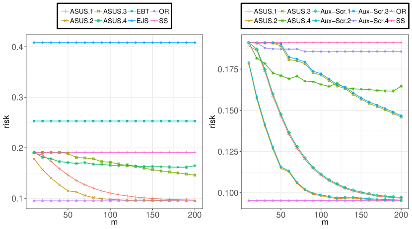
Figure 3: One-sample estimation with side information for scenario S1: Estimated risks of different estimators. Left: ASUS versus EBT and EJS. Right: ASUS verus Aux-Scr.

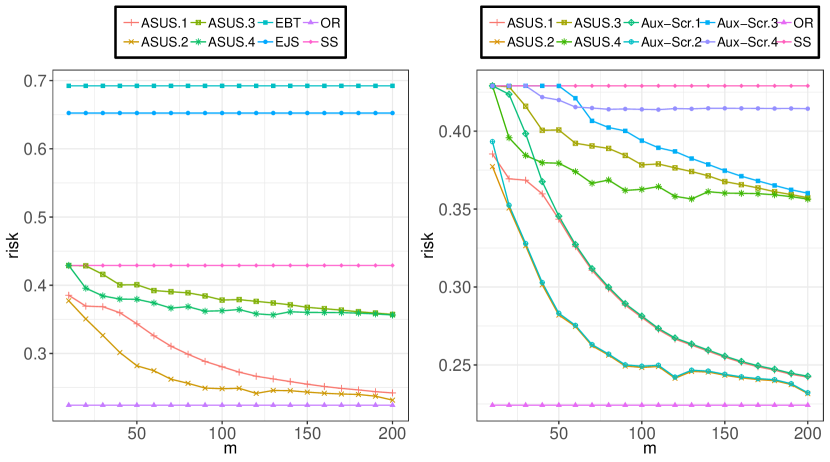
Figure 4: One-sample estimation with side information for scenario S2: Estimated risks of different estimators. Left: ASUS versus EBT and EJS. Right: ASUS verus Aux-Scr.

Table 1: One-sample estimation with side information: risk estimates and estimates of $\mathcal{T}$ for ASUS at $m=200$. Here $n_{k}^{{}^{\star}}=|\mathcal{I}_{k}^{\tau^{\star}}|$ and $n_{k}=|\widehat{\mathcal{I}}_{k}^{\tau}|$ for $k=1,2$.

		One-sample estimation with side information
		Scenario S1	Scenario S2
OR	$\tau^{\star}$	2	1.003
	$t_{1}^{\star}$, $t_{2}^{\star}$	4.114, 0.138	4.073, 0.133
	$n_{1}^{\star}$, $n_{2}^{\star}$	4750, 250	4008, 992
	risk	0.095	0.224
ASUS.1	$\tau$	1.342	0.979
	$t_{1}$, $t_{2}$	4.114, 0.107	4.073, 0.156
	$n_{1}$, $n_{2}$	4748, 252	4008, 992
	risk	0.097	0.243
ASUS.2	$\tau$	11.229	5.82
	$t_{1}$, $t_{2}$	4.115, 0.106	4.073, 0.137
	$n_{1}$, $n_{2}$	4748, 252	4008, 992
	risk	0.095	0.228
ASUS.3	$\tau$	1.777	1.778
	$t_{1}$, $t_{2}$	4.089, 0.662	3.422, 0.441
	$n_{1}$, $n_{2}$	4271, 729	3606, 1394
	risk	0.146	0.357
ASUS.4	$\tau$	7.785	8.524
	$t_{1}$, $t_{2}$	1.360, 3.653	0.745, 3.864
	$n_{1}$, $n_{2}$	1775, 3225	2249, 2751
	risk	0.165	0.356
Aux-Scr.1	risk	0.097	0.243
Aux-Scr.2	risk	0.095	0.232
Aux-Scr.3	risk	0.147	0.360
Aux-Scr.4	risk	0.186	0.414
SureShrink	risk	0.191	0.429
EBT	risk	0.253	0.692
EJS	risk	0.408	0.652

From the left panels of figures 3 and 4 we see that ASUS exhibits the best performance when compared against EBT, EJS and SureShrink estimators. In particular, ASUS.1, ASUS.2 outperform their counterparts ASUS.3, ASUS.4. This reveals how the usefulness of the latent sequence $\bm{\xi}$ would affect the performance of ASUS. Nonetheless, ASUS.3 and ASUS.4 still provide improvements over, and, crucially, are never worse than the SureShrink estimator. This reveals the impact of the accuracy of the auxiliary sequence $\bm{S}$ (in capturing the information in $\bm{\xi}$) on the performance of ASUS. The right panels of figures 3 and 4 present the risk comparison between ASUS and Aux-Scr using the auxiliary sequences $\bm{S}_{1},\ldots,\bm{S}_{4}$. Not surprisingly, ASUS and Aux-Scr have almost identical risk performance using the auxiliary sequences $\bm{S}_{1},\bm{S}_{2}$ and $\bm{S}_{3}$ for large $m$. As $m$ increases, the accuracy of these auxiliary sequences increase but the negative Bernoulli perturbations in $\bm{S}_{4}$ interferes with its magnitude so that a smaller $|S_{i4}|$ may correspond to a signal coordinate. The Aux-Scr procedure which discards observations based on the magnitude of the auxiliary sequence may miss important signal coordinates while relying on $\bm{S}_{4}$. ASUS, however, does not discard any observations and continues to exploit the available information in the noisy auxiliary sequences.

In table 1, we report risk estimates and estimates of $\mathcal{T}$ for ASUS when $m=200$. The estimates of the hyper-parameters of Aux-Scr are provided in table 2 of the supplementary material and we only report its risk estimates here in table 1. We can see that ASUS.1 and ASUS.2 choose similar thresholding hyper-parameters ($t_{1},t_{2}$) as those of the oracle estimator. Moreover, ASUS.4 demonstrates a lower estimation risk than Aux-Scr.4 using the same auxiliary sequence $\bm{S}_{4}$.

4.2.2 Two-sample estimation with side information

We consider the problem of estimating the difference of two Gaussian mean vectors. An auxiliary sequence can be constructed from data by following Example 3 in Section 2.2. We first simulate

$$\xi_{1i}\sim~{}(1-p_{1})\delta_{0}+p_{1}\,\mathrm{Unif}(3,7),\quad\xi_{2i}\sim~{}(1-p_{2})\delta_{0}+p_{2}\,\delta_{\{4\}},$$

where $\delta_{\{4\}}$ is the dirac delta at $4$ and then generate $\mu_{i,1}=\xi_{1i}+\eta_{1i}$ and $\mu_{i,2}=\xi_{2i}+\eta_{2i}$ with $\eta_{1i},\eta_{2i}\stackrel{{\scriptstyle i.i.d}}{{\sim}}N(0,0.01)$. The parameter of interest is $\bm{\theta}=\bm{\mu}_{1}-\bm{\mu}_{2}$ and the associated latent side information vector is $\bm{\xi}=\bm{\xi}_{1}-\bm{\xi}_{2}$. The observations based on the simulated mean vectors are generated as $U_{i}\sim~{}\mathrm{N}(\mu_{i,1},\sigma_{i,1}^{2}),\quad V_{i}\sim~{}\mathrm{N}(\mu_{i,2},\sigma_{i,2}^{2})$. Finally, the primary and auxiliary statistics are obtained as $Y_{i}=U_{i}-V_{i},\quad S_{i}=|U_{i}+\kappa_{i}V_{i}|$. We fix $p_{1}=n^{-0.6}$, $p_{2}=n^{-0.3}$, $\kappa_{i}=\sigma_{i,1}/\sigma_{i,2}$ and consider two scenarios where $\sigma_{i,1}=\sigma_{i,2}=1$ under scenario S1 and $(\sigma_{1,i}^{2},\sigma_{2,i}^{2})\stackrel{{\scriptstyle i.i.d}}{{\sim}}\mathrm{Unif}(0.1,1)$ under scenario S2. The estimates of risks are obtained by averaging over $N=1000$ replications. We vary $n$ from $500$ to $5000$ to investigate the impact of the strength of side information. The simulation results are reported in Table 2 and figure 5.

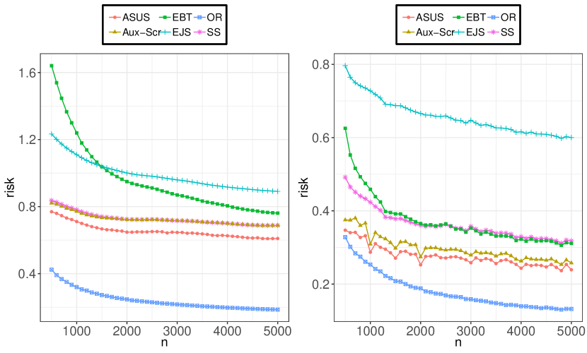
Figure 5: Two-sample estimation with side information: Average risks of different estimators. Left: Scenario S1 and Right: Scenario S2.

We see that ASUS uses the side information in $\bm{S}$ and exhibits the best performance across both scenarios. In scenario S2, the variances of $Y_{i}$ are smaller, which leads to an improved risk performance of ASUS over scenario S1. Similar to the previous simulation study, the risk of ASUS would not exceed the risk of the SureShrink estimator across both the scenarios. Different magnitudes of the thresholding hyper-parameters $(t_{1},t_{2})$ in table 2 further corroborates the importance of the auxiliary statistics $S_{i}$ in constructing groups with disparate sparsity levels and thereby improving the overall estimation accuracy. This is particularly true in the case of scenario S2 where EBT and SureShrink are competitive but ASUS is far more efficient because it has constructed two groups where one group holds majority of the signals and ASUS uses the smaller threshold $t_{2}$ to retain the signals. The other group holds majority of the noise wherein ASUS uses the larger threshold $t_{1}$ to shrink them to zero. Moreover, we notice that ASUS provides a better risk performance than Aux-Scr across both the scenarios. Using the side information in $\bm{S}$, Aux-Scr discards observations that have $|S_{i}|\leq\tau$ thereby eliminating some potentially information rich signal coordinates and thus returns a higher risk than ASUS.

Table 2: Two-sample estimation with side information: risk estimates and estimates of $\mathcal{T}$ for ASUS at $n=5000$. Here $n_{k}^{{}^{\star}}=|\mathcal{I}_{k}^{\tau^{\star}}|$ and $n_{k}=|\widehat{\mathcal{I}}_{k}^{\tau}|$ for $k=1,2$.

		Two-sample estimation with side information
		Scenario S1	Scenario S2
OR	$\tau^{\star}$	1.947	1.363
	$t_{1}^{\star}$, $t_{2}^{\star}$	4.106, 0.137	4.106, 0.424
	$n_{1}^{\star}$, $n_{2}^{\star}$	4584, 416	4583, 417
	risk	0.185	0.132
ASUS	$\tau$	3.167	2.504
	$t_{1}$, $t_{2}$	1.223, 0.253	3.058, 0.323
	$n_{1}$, $n_{2}$	4570, 430	4195, 805
	risk	0.610	0.239
Aux-Scr	$\tau$	14.385	2.768
	$t_{1}$, $t_{2}$	0.955, 0.002	5.708, 0.498
	$n_{1}$, $n_{2}$	4991, 9	3681, 1319
	risk	0.688	0.258
SureShrink	risk	0.688	0.318
EBT	risk	0.761	0.311
EJS	risk	0.891	0.600

4.3 Analysis of RNA sequence data

We compare the performance of ASUS against the SureShrink (SS) estimator for analysis of the RNA sequence data described in the introduction. The goal is to estimate the true expression levels $\bm{\theta}$ of the $n$ genes that are infected with VZV strain. Through previous studies conducted in the lab, expression levels corresponding to other four experimental conditions, including uninfected cells (C1, 3 replicates), a fibrosarcoma cell line (C2, 3 replicates) and cells treated with interferons gamma (C3, 2 replicates), alpha (C4, 3 replicates), were also collected. Let $X_{i}$ be the mean expression level of gene $i$ across the four experimental conditions. Set $S_{i}=|X_{i}|$ with $K=2$. Let $\hat{\theta}_{i}^{S}(t)$ denote the SureShrink estimator of $\theta_{i}$ based on $Y_{i}$, the mean expression level of gene $i$ under the VZV condition. The standard deviation $\sigma_{i}$ for the mean expression level pertaining to gene $i$ across the 3 replicates of the VZV strain is derived from the study conducted in Sen et al. (2018).

On the right panel of Figure 6, the dotted line represents the minimum of the SURE risk of $\hat{\bm{\theta}}^{S}(t)$, which is minimized at $t=0.61$. The solid line represents the minimum of the SURE risk of a class of two-group estimators over a grid of $\tau$ values. ASUS chooses $\tau$ that minimizes the SURE risk (the red dot in figure 6). The resulting risk is $1.99\%$ at $\hat{\mathcal{T}}=(1.25,1.16,0)$, a significant reduction compared to the risk estimate of $3.69\%$ for $\hat{\bm{\theta}}^{S}(t)$. In order to evaluate the results in a predictive framework, we next use only two replicates of the VZV strain for calibrating the hyper-parameters and calculate the prediction errors based on the hold out third replicate. The risk reduction by ASUS over SureShrink is about $30\%$.

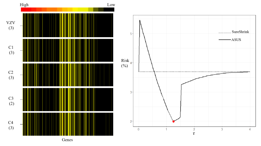
Figure 6: Left: Heat map showing the following from top to bottom: average expression levels of VZV, C1, C2, C3 and C4 across their respective replicates (in parenthesis). Right: SURE estimate of the risk of $\hat{\theta}^{S}_{i}(t)$ at $t=0.61$ versus an unbiased estimate of the risk of ASUS for different values of $\tau$.

In this example, a reduction in risk is possible because ASUS has efficiently exploited the sparsity information about $\bm{\theta}$ encoded by $\bm{S}$. This can be seen, for example, from (i) the stark contrast between the magnitudes of thresholding hyper-parameters $t_{1},t_{2}$ for the two groups in table 3 and (ii) the heat maps in figure 6 where the genes expressions under the four experimental conditions follow the expression pattern of VZV. Moreover, the risk of Aux-Scr for this example was seen to be no better than the SureShrink estimator and thus has been excluded from the results reported in table 3. Figure 7(a) presents the distribution of gene expression for genes that belong to groups $\widehat{\mathcal{I}}_{1}^{\tau}$ and $\widehat{\mathcal{I}}_{2}^{\tau}$. ASUS exploits the side information in $\bm{S}$ to partition the estimation units into two groups with very different sparsity levels and therefore returns a much smaller risk.

(a)

(b)

Figure 7: (a) Histogram of gene expressions for VZV. Group 1 is $\widehat{\mathcal{I}}^{\tau}_{2}$ and Group 0 is $\widehat{\mathcal{I}}^{\tau}_{1}$. (b) A network of 20 new genes highlighted in black with their interaction partners.

Table 3: Summary of SureShrink and ASUS methods (RNA-Seq data). $n_{k}=|\widehat{\mathcal{I}}_{k}^{\tau}|$ for $k=1,2$.

		RNA Seq
	$n$	53,216
SureShrink	$t$	0.61
	SURE estimate	3.69
ASUS	$\tau$	1.25
	$t_{1}$	1.16
	$t_{2}$	0
	$n_{1}$	39,535
	$n_{2}$	13,681
	SURE estimate	1.99

The ASUS estimator $\hat{\bm{\theta}}^{SI}(\hat{\mathcal{T}})$ results in the discovery of $114$ new genes than those discovered by using $\hat{\bm{\theta}}^{SI}(t)$. Figure 7(b) shows the network of protein-protein interactions of 20 such genes. The interaction network is generated using NetworkAnalyst (Xia et al., 2015) that maps the chosen genes to a comprehensive high-quality protein-protein interaction (PPI) database based on InnateDB. A search algorithm is then performed to identify first-order neighbors (genes that directly interact with a given gene) for each of these mapped genes. The resulting nodes and their interaction partners are returned to build the network. In case of the RNA-Seq data, the interaction network of the 20 new genes indicates that ASUS may help reveal important biological synergies between genes that have a high estimated expression level for VZV and other genes in the human genome.

5 Discussion

In high-dimensional estimation and testing problems, the sparsity structure can be encoded in various ways; we have considered three basic settings where the structural information on sparsity may be extracted from (i) prior or domain-specific knowledge, (ii) covariate sequence based on the same data, or (iii) summary statistics based on secondary data sources. This article develops a general integrative framework for sparse estimation that is capable of handling all three scenarios. We use higher-order minimax optimality tools to establish the adaptivity and robustness of ASUS. Numerical studies using both simulated and real data corroborate the improvement of ASUS over existing methods.

We conclude the article with a discussion of several open issues. Firstly, in large-scale compound estimation problems, various data structures such as sparsity, heteroscedasticity, dependency and hierarchy are often available alongside the primary summary statistics. ASUS can only handle the sparsity structure; and it is desirable to develop a unified framework that can effectively incorporate other types of structures into inference. New theoretical frameworks will be needed to characterize the usefulness of various types of side information and to establish precise conditions under which the new integrative method is asymptotically optimal. Secondly, in situations where there are multiple auxiliary sequences, it is unclear how to modify the ASUS framework to construct groups using an auxiliary matrix. The computation involved in the search for the optimal group-wise thresholds, which requires the evaluation of the SURE function for every possible combination of group-wise thresholds, quickly becomes prohibitively expensive as the number of columns increases. Finally, the higher dimension would affect the stability of an integrative procedure adversely. A promising idea for handling multiple auxiliary sequences is to construct a new auxiliary sequence that represents the “optimal use” of all available side information. However, the search for this optimal direction of projection is quite challenging. It would be of great interest to explore these directions in future research.

Acknowledgments

We thank Ann Arvin and Nandini Sen for helpful discussions on the virology application. We thank the AE and two referees for the constructive suggestions that have greatly helped to improve the presentation of the paper. In particular, we are grateful to an excellent comment from a referee that leads to the Bayesian interpretation of ASUS in Section 2.4.

References

- Abramovich et al. (2006) Abramovich, F., Y. Benjamini, D. L. Donoho, and I. M. Johnstone (2006). Adapting to unknown sparsity by controlling the false discovery rate. Ann. Statist. 34, 584–653.
- Abramovich et al. (2007) Abramovich, F., V. Grinshtein, M. Pensky, et al. (2007). On optimality of bayesian testimation in the normal means problem. The Annals of Statistics 35(5), 2261–2286.
- Bickel (1983) Bickel, P. (1983). Minimax estimation of a normal mean subject to doing well at a point. Recent Advances in Statistics (MH Rizvi, JS Rustagi, and D. Siegmund, eds.), Academic Press, New York, 511–528.
- Brown (2008) Brown, L. D. (2008). In-season prediction of batting averages: A field test of empirical bayes and bayes methodologies. The Annals of Applied Statistics, 113–152.
- Brown and Greenshtein (2009) Brown, L. D. and E. Greenshtein (2009). Nonparametric empirical bayes and compound decision approaches to estimation of a high-dimensional vector of normal means. The Annals of Statistics, 1685–1704.
- Brown et al. (2017) Brown, L. D., G. Mukherjee, and A. Weinstein (2017). Empirical bayes estimates for a 2-way cross-classified additive model. Annals of Statistics (forthcoming).
- Cai et al. (2018) Cai, T., W. Sun, and W. Wang (2018+). Cars: Covariate assisted ranking and screening for large-scale two-sample inference. To appear: Journal of the Royal Statistical Society, Series B.
- Cai et al. (2014) Cai, T. T., M. Low, and Z. Ma (2014). Adaptive confidence bands for nonparametric regression functions. Journal of the American Statistical Association 109(507), 1054–1070.
- Cai and Sun (2017) Cai, T. T. and W. Sun (2017). Optimal screening and discovery of sparse signals with applications to multistage high throughput studies. Journal of the Royal Statistical Society: Series B (Statistical Methodology) 79(1), 197–223.
- Calvano et al. (2005) Calvano, S. E., W. Xiao, D. R. Richards, R. M. Felciano, H. V. Baker, R. J. Cho, R. O. Chen, B. H. Brownstein, J. P. Cobb, S. K. Tschoeke, et al. (2005). A network-based analysis of systemic inflammation in humans. Nature 437(7061), 1032–1037.
- Collier et al. (2017) Collier, O., L. Comminges, A. B. Tsybakov, et al. (2017). Minimax estimation of linear and quadratic functionals on sparsity classes. The Annals of Statistics 45(3), 923–958.
- Cover and Thomas (2012) Cover, T. M. and J. A. Thomas (2012). Elements of information theory. John Wiley & Sons.
- Donoho and Jin (2004) Donoho, D. and J. Jin (2004). Higher criticism for detecting sparse heterogeneous mixtures. Ann. Statist. 32, 962–994.
- Donoho and Johnstone (1995) Donoho, D. L. and I. M. Johnstone (1995). Adapting to unknown smoothness via wavelet shrinkage. Journal of the american statistical association 90(432), 1200–1224.
- Donoho et al. (1998) Donoho, D. L., I. M. Johnstone, et al. (1998). Minimax estimation via wavelet shrinkage. The annals of Statistics 26(3), 879–921.
- Efron (2011) Efron, B. (2011). Tweedie’s formula and selection bias. Journal of the American Statistical Association 106(496), 1602–1614.
- Erickson et al. (2005) Erickson, S., C. Sabatti, et al. (2005). Empirical bayes estimation of a sparse vector of gene expression changes. Statistical applications in genetics and molecular biology 4(1), 1132.
- Holland et al. (2016) Holland, D., Y. Wang, W. K. Thompson, A. Schork, C.-H. Chen, M.-T. Lo, A. Witoelar, T. Werge, M. O’Donovan, O. A. Andreassen, et al. (2016). Estimating effect sizes and expected replication probabilities from gwas summary statistics. Frontiers in genetics 7.
- Johnstone (1994) Johnstone, I. M. (1994). On minimax estimation of a sparse normal mean vector. The Annals of Statistics, 271–289.
- Johnstone (2015) Johnstone, I. M. (2015). Gaussian estimation:sequence and wavelet models. Draft version.
- Johnstone and Silverman (1997) Johnstone, I. M. and B. W. Silverman (1997). Wavelet threshold estimators for data with correlated noise. Journal of the royal statistical society: series B (statistical methodology) 59(2), 319–351.
- Johnstone and Silverman (2004) Johnstone, I. M. and B. W. Silverman (2004). Needles and straw in haystacks: Empirical bayes estimates of possibly sparse sequences. Annals of Statistics, 1594–1649.
- Ke et al. (2014) Ke, T., J. Jin, and J. Fan (2014). Covariance assisted screening and estimation. Annals of statistics 42(6), 2202.
- Kou and Yang (2015) Kou, S. and J. J. Yang (2015). Optimal shrinkage estimation in heteroscedastic hierarchical linear models. arXiv preprint arXiv:1503.06262.
- Li et al. (2008) Li, C., M. Li, E. M. Lange, and R. M. Watanabe (2008). Prioritized subset analysis: improving power in genome-wide association studies. Human heredity 65(3), 129–141.
- Mallat (2008) Mallat, S. (2008). A Wavelet Tour of Signal Processing, Third Edition: The Sparse Way (3rd ed.). Academic Press.
- Matsui (2013) Matsui, S. (2013). Genomic biomarkers for personalized medicine: development and validation in clinical studies. Computational and mathematical methods in medicine 2013.
- Mukherjee and Johnstone (2015) Mukherjee, G. and I. M. Johnstone (2015). Exact minimax estimation of the predictive density in sparse gaussian models. Annals of statistics 43(3), 937.
- Sen et al. (2018) Sen, N., P. Sung, A. Panda, and A. M. Arvin (2018). Distinctive roles for type i and type ii interferons and interferon regulatory factors in the host cell defense against varicella-zoster virus. Journal of virology, JVI–01151.
- Sun and Wei (2011) Sun, W. and Z. Wei (2011). Multiple testing for pattern identification, with applications to microarray time-course experiments. Journal of the American Statistical Association 106(493), 73–88.
- Tan et al. (2015) Tan, Z. et al. (2015). Improved minimax estimation of a multivariate normal mean under heteroscedasticity. Bernoulli 21(1), 574–603.
- Tibshirani et al. (2014) Tibshirani, R. J. et al. (2014). Adaptive piecewise polynomial estimation via trend filtering. The Annals of Statistics 42(1), 285–323.
- Watanabe et al. (2015) Watanabe, S., S. Kuzuoka, and V. Y. Tan (2015). Nonasymptotic and second-order achievability bounds for coding with side-information. IEEE Transactions on Information Theory 61(4), 1574–1605.
- Weinstein et al. (2018) Weinstein, A., Z. Ma, L. D. Brown, and C.-H. Zhang (2018). Group-linear empirical bayes estimates for a heteroscedastic normal mean. Journal of the American Statistical Association, 1–13.
- Wyner (1975) Wyner, A. (1975). On source coding with side information at the decoder. IEEE Transactions on Information Theory 21(3), 294–300.
- Xia et al. (2015) Xia, J., E. E. Gill, and R. E. Hancock (2015). Networkanalyst for statistical, visual and network-based meta-analysis of gene expression data. Nature protocols 10(6), 823–844.
- Xie et al. (2012) Xie, X., S. Kou, and L. D. Brown (2012). Sure estimates for a heteroscedastic hierarchical model. Journal of the American Statistical Association 107(500), 1465–1479.
- Zerboni et al. (2014) Zerboni, L., N. Sen, S. L. Oliver, and A. M. Arvin (2014). Molecular mechanisms of varicella zoster virus pathogenesis. Nature Reviews Microbiology 12(3), 197–210.