Certifying Quantum Randomness by Probability Estimation

Abstract

We introduce probability estimation, a broadly applicable framework to certify randomness in a finite sequence of measurement results without assuming that these results are independent and identically distributed. Probability estimation can take advantage of verifiable physical constraints, and the certification is with respect to classical side information. Examples include randomness from single-photon measurements and device-independent randomness from Bell tests. Advantages of probability estimation include adaptability to changing experimental conditions, unproblematic early stopping when goals are achieved, optimal randomness rates, applicability to Bell tests with small violations, and unsurpassed finite-data efficiency. We greatly reduce latencies for producing random bits and formulate an associated rate-tradeoff problem of independent interest. We also show that the latency is determined by an information-theoretic measure of nonlocality rather than the Bell violation.

Randomness is a key enabling resource for computation and communication. Besides being required for Monte-Carlo simulations and statistical sampling, private random bits are needed for initiating authenticated connections and establishing shared keys, both common tasks for browsers, servers and other online entities Paar and Pelzl (2010). Public random bits from “randomness beacons” have applications to fair resource sharing Fischer (2011) and can seed private randomness sources based on quantum mechanics Pironio and Massar (2013). Common requirements for random bits are that they are unpredictable to all before they are generated, and private to the users before they are published.

Quantum mechanics provides natural opportunities for generating randomness. The best known example involves measuring a two-level system that is in an equal superposition of its two levels. A disadvantage of such schemes is that they require trust in the measurement apparatus, and undiagnosed failures are always a possibility. This disadvantage is overcome by a loophole-free Bell test Colbeck (2007); Colbeck and Kent (2011), which can generate output whose randomness can be certified solely by statistical tests of setting and outcome frequencies. The devices preparing the quantum states and performing the measurements may come from an untrusted source. This strategy for certified randomness generation is known as device-independent randomness generation (DIRG).

Loophole-free Bell tests have been realized with nitrogen-vacancy (NV) centers Hensen et al. (2015), with atoms Rosenfeld et al. (2017) and with photons Giustina et al. (2015); Shalm et al. (2015), enabling the possibility of full experimental implementations of DIRG. However, for NV centers and atoms, the rate of trials is too low, and for photons, the violation per trial is too small. As a result, previously available DIRG protocols Pironio et al. (2010); Vazirani and Vidick (2012); Pironio and Massar (2013); Fehr et al. (2013); Miller and Shi (2016, 2017); Chung et al. (2014); Coudron and Yuen (2014); Arnon-Friedman et al. (2018); Nieto-Silleras et al. (2018) are not ready for implementation with current loophole-free Bell tests. These protocols do not achieve good finite-data efficiency and therefore require an impractical number of trials. Experimental techniques will improve, but for many applications of randomness generation, including randomness beacons and key generation, it is desirable to achieve finite-data efficiency that is as high as possible, since these applications often require short blocks of fresh random bits with minimum delay or latency.

Excellent finite-data efficiency was achieved by a method that we described and implemented in Refs. Bierhorst et al. (2017, 2018), which reduced the time required for generating $1024$ low-error random bits with respect to classical side information from hours to minutes for a state-of-the-art photonic loophole-free Bell test. The method in Refs. Bierhorst et al. (2017, 2018) is based on the prediction-based ratio (PBR) analysis Zhang et al. (2011) for hypothesis tests of local realism. Specifically, in Refs. Bierhorst et al. (2017, 2018) we established a connection between the PBR-based $p$-value and the amount of randomness certified against classical side information. The basis for success of the method of Refs. Bierhorst et al. (2017, 2018) motivates our development of probability estimation for randomness certification, with better finite-data efficiency and with broader applications.

In the probability estimation framework, the amount of certified randomness is directly estimated without relying on hypothesis tests of local realism. To certify randomness, we first obtain a bound on the conditional probability of the observed outcomes given the chosen settings, valid for all classical side information. Then we show how to obtain conditional entropy estimates from this bound to quantify the number of extractable random bits König et al. (2009). By focusing on data-dependent probability estimates, we are able to take advantage of powerful statistical techniques to obtain the desired bound. The statistical techniques are based on test supermartingales Shafer et al. (2011) and Markov’s bounds. Probability estimation inherits several features of the theory of test supermartingales. For example, probability estimation has no independence or stationarity requirement on the probability distribution of trial results. Also, probability estimation supports stopping the experiment early, as soon as the randomness goal is achieved.

Probability estimation is broadly applicable. In particular it is not limited to device-independent scenarios and can be applied to traditional randomness generation with quantum devices. Such applications are enabled by the notion of models, which are sets of probability distributions that capture verified, physical constraints on device behavior. In the case of Bell tests, these constraints include the familiar non-signaling conditions Popescu and Rohrlich (1994); Barrett et al. (2005). In the case of two-level systems such as polarized photons, the constraints can capture that measurement angles are within a known range, for example.

In this paper, we first describe the technical features of probability estimation and the main results that enable its practical use. We propose a general information-theoretic rate-tradeoff problem that closely relates to finite-data efficiency. We then show how the general theoretical concepts are instantiated in experimentally relevant examples involving Bell-test configurations. We demonstrate advantages of probability estimation such as its optimal asymptotic randomness rates and show large improvements in finite-data efficiency, which corresponds to great reductions in latency.

Theory. Consider an experiment with “inputs” $\mathbf{Z}$ and “outputs” $\mathbf{C}$. The inputs normally consist of the random choices made for measurement settings but may include choices of state preparations such as in the protocols of Refs. Lunghi et al. (2015); Himbeeck et al. (2017). The outputs consist of the corresponding measurement outcomes. In the cases of interest, the inputs and outputs are obtained in a sequence of $n$ time-ordered trials, where the $i$’th trial has input $Z_{i}$ and output $C_{i}$, and $\mathbf{Z}=(Z_{i})_{i=1}^{n}$ and $\mathbf{C}=(C_{i})_{i=1}^{n}$. We assume that $Z_{i}$ and $C_{i}$ are countable-valued. We refer to the trial inputs and outputs collectively as the trial “results”, and to the trials preceding the upcoming one as the “past”. The party with respect to which the randomness is intended to be unpredictable is represented by an external classical system, whose initial state before the experiment may be correlated with the devices used. The classical system carries the side information $E$, which is assumed to be countable-valued. After the experiment, the joint of $\mathbf{Z}$, $\mathbf{C}$ and $E$ is described by a probability distribution $\mu$. The upper-case symbols introduced in this paragraph are treated as random variables. As is conventional, their values are denoted by the corresponding lower-case symbols.

The amount of extractable uniform randomness in $\mathbf{C}$ conditional on both $\mathbf{Z}$ and $E$ is quantified by the (classical) smooth conditional min-entropy $H_{\min}^{\epsilon}(\mathbf{C}|\mathbf{Z}E)_{\mu}$ where $\epsilon$ is the “error bound” (or “smoothness”) and $\mu$ is the joint distribution of $\mathbf{Z}$, $\mathbf{C}$ and $E$. One way to define the smooth conditional min-entropy is with the conditional guessing probability $P_{\mathrm{guess}}(\mathbf{C}|\mathbf{Z}E)_{\mu}$ defined as the average over values $\mathbf{z}$ and $e$ of the maximum conditional probability $\max_{\mathbf{c}}\mu(\mathbf{c}|\mathbf{z}e)$. The $\epsilon$-smooth conditional min-entropy $H_{\min}^{\epsilon}(\mathbf{C}|\mathbf{Z}E)_{\mu}$ is the greatest lower bound of $-\log_{2}P_{\mathrm{guess}}(\mathbf{C}|\mathbf{Z}E)_{\mu^{\prime}}$ for all distributions $\mu^{\prime}$ within total-variation distance $\epsilon$ of $\mu$. Our goal is to obtain lower bounds on $H_{\min}^{\epsilon}(\mathbf{C}|\mathbf{Z}E)_{\mu}$ with probability estimation.

The application of probability estimation requires a notion of models. A model $\mathcal{H}$ for an experiment is defined as the set of all probability distributions of $\mathbf{Z}$ and $\mathbf{C}$ achievable in the experiment conditionally on values $e$ of $E$. If a joint distribution $\mu$ of $\mathbf{Z}$, $\mathbf{C}$ and $E$ satisfies that for all $e$, the conditional distributions $\mu(\mathbf{C}\mathbf{Z}|e)$, considered as distributions of $\mathbf{Z}$ and $\mathbf{C}$, are in $\mathcal{H}$, we say that the distribution $\mu$ satisfies the model $\mathcal{H}$.

To apply probability estimation to an experiment consisting of $n$ time-ordered trials, we construct the model $\mathcal{H}$ for the experiment as a chain of models $\mathcal{C}_{i}$ for each individual trial $i$ in the experiment. The trial model $\mathcal{C}_{i}$ is defined as the set of all probability distributions of trial results $C_{i}Z_{i}$ achievable at the $i$’th trial conditionally on both the past trial results and the side information $E$. For example, for Bell tests, $\mathcal{C}_{i}$ may be the set of non-signaling distributions with uniformly random inputs. Let $\mathbf{z}_{<i}=(z_{j})_{j=1}^{i-1}$ and $\mathbf{c}_{<i}=(c_{j})_{j=1}^{i-1}$ be the results before the $i$’th trial. The sequences $\mathbf{z}_{\leq i}$ and $\mathbf{c}_{\leq i}$ are defined similarly. The chained model $\mathcal{H}$ consists of all conditional distributions $\mu(\mathbf{C}\mathbf{Z}|e)$ satisfying the following two conditions. First, at each trial $i$ the conditional distributions $\mu(C_{i}Z_{i}|\mathbf{c}_{<i}\mathbf{z}_{<i}e)$ for all $\mathbf{c}_{<i}$, $\mathbf{z}_{<i}$ and $e$ are in the trial model $\mathcal{C}_{i}$. Second, at each trial $i$ the input $Z_{i}$ is independent of the past outputs $\mathbf{C}_{<i}$ given $E$ and the past inputs $\mathbf{Z}_{<i}$. The second condition prevents leaking information about the past outputs through the future inputs, which is necessary for certifying randomness in the outputs $\mathbf{C}$ conditional on both the inputs $\mathbf{Z}$ and the side information $E$. In the common situation where the inputs are chosen independently with distributions known before the experiment, the second condition is always satisfied.

Since the model $\mathcal{H}$ consists of all conditional distributions $\mu(\mathbf{C}\mathbf{Z}|e)$ regardless of the value $e$, the analyses in the next paragraph apply to the worst-case conditional distribution over $e$. To simplify notation we normally write the distribution $\mu(\mathbf{C}\mathbf{Z}|e)$ conditional on $e$ as $\mu_{e}(\mathbf{C}\mathbf{Z})$, abbreviated as $\mu_{e}$.

To estimate the conditional probability $\mu_{e}(\mathbf{c}|\mathbf{z})$, we design trial-wise probability estimation factors (PEFs) and multiply them. Consider a generic trial with trial model $\mathcal{C}$, where for generic trials, we omit the trial index. Let $\beta>0$. A PEF with power $\beta$ for $\mathcal{C}$ is a function $F:cz\mapsto F(cz)\geq 0$ such that for all $\sigma\in\mathcal{C}$, $\mathbb{E}_{\sigma}\big{(}F(CZ)\sigma(C|Z)^{\beta}\big{)}\leq 1$, where $\mathbb{E}$ denotes the expectation functional. Note that $F(cz)=1$ for all $cz$ defines a valid PEF with each positive power. For each $i$, let $F_{i}$ be a PEF with power $\beta$ for the $i$’th trial, where the PEF can be chosen adaptively based on the past results $\mathbf{c}_{<i}\mathbf{z}_{<i}$. Other information from the past may also be used, see Ref. Knill et al. (2017). Let $T_{0}=1$ and $T_{i}=\prod_{j=1}^{i}F_{j}(C_{j}Z_{j})$. The final value $T_{n}$ of the running product $T_{i}$, where $n$ is the total number of trials in the experiment, determines the probability estimate. Specifically, for each value $e$ of $E$, each $\mu_{e}$ in the chained model $\mathcal{H}$, and $\epsilon>0$, we have

$$\mathbb{P}_{\mu_{e}}\big{(}\mu_{e}(\mathbf{C}|\mathbf{Z})\geq U(\mathbf{C}\mathbf{Z})\big{)}\leq\epsilon,$$ (1)

where $\mathbb{P}_{\mu_{e}}$ denotes the probability according to the distribution $\mu_{e}$ and $U(\mathbf{C}\mathbf{Z})=(\epsilon T_{n})^{-1/\beta}$. The proof of Eq. (1) is given in Appendix C.1. The meaning of Eq. (1) is as follows: For each $e$ and each $\mu_{e}\in\mathcal{H}$, the probability that $\mathbf{C}$ and $\mathbf{Z}$ take values $\mathbf{c}$ and $\mathbf{z}$ for which $U(\mathbf{C}=\mathbf{c},\mathbf{Z}=\mathbf{z})\leq\mu_{e}(\mathbf{C}=\mathbf{c}|\mathbf{Z}=\mathbf{z})$ is at most $\epsilon$. This defines $U(\mathbf{C}\mathbf{Z})=(\epsilon T_{n})^{-1/\beta}$ as a level-$\epsilon$ probability estimator.

A main theorem of probability estimation is the connection between probability estimators and conditional min-entropy estimators, which is formalized as follows:

Theorem 1.

Suppose that the joint distribution $\mu$ of $\mathbf{Z}$, $\mathbf{C}$ and $E$ satisfies the chained model $\mathcal{H}$. Let $1\geq\kappa,\epsilon>0$ and $1\geq p\geq 1/|\mathrm{Rng}(\mathbf{C})|$, where $|\mathrm{Rng}(\mathbf{C})|$ is the number of possible outputs. Define $\{\phi\}$ to be the event that $T_{n}\geq 1/(p^{\beta}\epsilon)$, and let $\kappa\leq\mathbb{P}_{\mu}(\phi)$. Then the smooth conditional min-entropy satisfies

$$H_{\min}^{\epsilon}(\mathbf{C}|\mathbf{Z}E;\phi)\geq-\log_{2}(p/\kappa^{1+1/\beta}).$$

The probability of the event $\{\phi\}$ can be interpreted as the probability that the experiment succeeds, and $\kappa$ is an assumed lower bound on the success probability. The theorem is proven in Appendix C.2.

When constructing PEFs, the power $\beta>0$ must be decided before the experiment and cannot be adapted. Thm. 1 requires that $p$, $\epsilon$ and $\kappa$ also be chosen beforehand, and success of the experiment requires $T_{n}\geq 1/(p^{\beta}\epsilon)$, or equivalently,

$$\log_{2}(T_{n})/\beta+\log_{2}(\epsilon)/\beta\geq-\log_{2}(p).$$ (2)

Since $\log_{2}(T_{n})=\sum_{i}\log_{2}(F_{i})$, before the experiment we choose PEFs in order to aim for large expected values of the logarithms of the PEFs $F_{i}$. Consider a generic next trial with results $CZ$ and model $\mathcal{C}$. Based on prior calibrations or the frequencies of observed results in past trials, we can determine a distribution $\nu\in\mathcal{C}$ that is a good approximation to the distribution of the next trial’s results $CZ$. Many experiments are designed so that each trial’s distribution is close to $\nu$. The PEF can be optimized for this distribution but, by definition, is valid regardless of the actual distribution of the next trial in $\mathcal{C}$. Thus, one way to optimize PEFs before the next trial is as follows:

$$\begin{array}[b]{ll}\textrm{Max:}&\mathbb{E}_{\nu}\big{(}n\log_{2}(F(CZ))/\beta+\log_{2}(\epsilon)/\beta\big{)}\\ \textrm{With:}&\sum_{cz}F(cz)\sigma(c|z)^{\beta}\sigma(cz)\leq 1\textrm{\ for all $\sigma\in\mathcal{C}$},\\ &F(cz)\geq 0,\textrm{\ for all $cz$}.\end{array}$$ (3)

The objective function is strictly concave and the constraints are linear, so there is a unique maximum, which can be found by convex programming. More details are available in Appendix E.

Before the experiment, one can also optimize the objective function in Eq. (3) with respect to the power $\beta$. During the experiment $\epsilon$ and $\beta$ are fixed, so it suffices to maximize $\mathbb{E}_{\nu}\big{(}\log_{2}(F(CZ))\big{)}$. If during the experiment, the running product $T_{i}$ with $i<n$ exceeds the target $1/(p^{\beta}\epsilon)$, we can set future PEFs to $F(CZ)=1$, which is a valid PEF with power $\beta$. This ensures that $T_{n}=T_{i}$ and is equivalent to stopping the experiment after trial $i$. Since the target needs to be set conservatively in order to make the actual experiment succeed with high probability, this can result in a significant reduction in the number of trials actually executed.

A question is how PEFs perform asymptotically for a stable experiment. This question is answered by determining the rate per trial of entropy production assuming constant $\epsilon$ and $\kappa$ independent of the number of trials. In view of Thm. 1, after $n$ trials the entropy rate is given by $\big{(}-\log_{2}(p)+\log_{2}(\kappa^{1+1/\beta})\big{)}/n$. Considering Eq. (2), when $n$ is large the entropy rate is dominated by $\log_{2}(T_{n})/(n\beta)$, which is equal to $\sum_{i=1}^{n}\log_{2}(F_{i})/(n\beta)$. Therefore, if each trial has distribution $\nu$ and each trial model is the same $\mathcal{C}$, then in the limit of large $n$ the asymptotic entropy rate witnessed by a PEF $F$ with power $\beta$ is given by $\mathbb{E}_{\nu}\big{(}\log_{2}(F(CZ))/\beta\big{)}$. Define the rate

$$g(\beta)=\sup_{F}\mathbb{E}_{\nu}\big{(}\log_{2}(F(CZ))/\beta\big{)},$$ (4)

where the supremum is over PEFs $F$ with power $\beta$ for $\mathcal{C}$. The maximum asymptotic entropy rate at constant $\epsilon$ and $\kappa$ witnessed by PEFs is $g_{0}=\sup_{\beta>0}g(\beta)$. The rate $g(\beta)$ is non-increasing in $\beta$ (see Appendix D), so $g_{0}$ is determined by the limit as $\beta$ goes to zero. A theorem proven in Ref. Knill et al. (2017) is that $g_{0}$ is the worst-case conditional entropy $H(C|ZE)$ over joint distributions of $CZE$ allowed by $\mathcal{C}$ with marginal $\nu$. Since this is a tight upper bound on the asymptotic randomness rate Tomamichel et al. (2009), probability estimation is asymptotically optimal and we identify $g_{0}$ as the asymptotic randomness rate. We also remark that probability estimation enables exponential expansion of input randomness Knill et al. (2017).

For finite data and applications requiring fresh blocks of randomness, the rate $g_{0}$ is not achieved. To understand why, consider the problem of certifying a fixed number of bits $b$ of randomness at error bound $\epsilon$ and with as few trials as possible, where each trial has distribution $\nu$. In view of Thm. 1, the PEF optimization problem in Eq. (3), and the definition of $g(\beta)$ in Eq. (4), $n$ needs to be sufficiently large so that

$$ng(\beta)+\log_{2}(\epsilon)/\beta+(1+1/\beta)\log_{2}(\kappa)\geq b.$$ (5)

The left-hand side is maximized at positive $\beta$, whereas $g(\beta)$ increases to $g_{0}$ as $\beta$ goes to zero. As a result the best actual rate $b/n$ is less than $g_{0}$.

Setting $\kappa=1$ in Eq. (5) shows that the number of trials $n$ must exceed $-\log_{2}(\epsilon)/(\beta g(\beta))$ before randomness can be produced, which suggests that the maximum of $\beta g(\beta)$ is a good indicator of finite-data performance. Another way to arrive at this quantity is to consider $\epsilon=2^{-\gamma n}$, where $\gamma>0$ is the “certificate rate”. Given $\nu$ and the trial model, we can ask for the maximum certificate rate for which it is possible to have positive entropy rate at $\kappa=1$. It follows from Eq. (5) with $\kappa=1$ that this rate is at most

$$\gamma_{\textrm{PEF}}=\sup_{\beta>0}\beta g(\beta).$$ (6)

We propose a general information-theoretic rate-tradeoff problem given trial model $\mathcal{C}$ and $\nu\in\mathcal{C}$: For a given certificate rate $\gamma$, determine the supremum of the entropy rates achievable by protocols. Eq. (5) implies lower bounds on the resulting tradeoff curve.

Our protocol assumes classical-only side information. There are more costly DIRG protocols that handle quantum side information Vazirani and Vidick (2012); Miller and Shi (2016, 2017); Chung et al. (2014); Coudron and Yuen (2014); Arnon-Friedman et al. (2018), but verifying that side information is effectively classical only requires confirming that the quantum devices used in the experiment have no long-term quantum memory. Verifying the absence of long-term quantum memory in current experiments is possibly less difficult than ensuring that there are no backdoors or information leaks in the experiment’s hardware and software.

Applications. We consider DIRG with the standard two-party, two-setting, two-outcome Bell-test configuration Clauser et al. (1969). The parties are labeled A and B. In each trial, a source prepares a state shared between the parties, and each party chooses a random setting (their input) and obtains a measurement outcome (their output). We write $Z=XY$, where $X$ and $Y$ are the inputs of A and B, and $C=AB$, where $A$ and $B$ are the respective outputs. For this configuration, $A,B,X,Y\in\{0,1\}$.

Consider the trial model $\mathcal{N}$ consisting of distributions of $ABXY$ with uniformly random inputs and satisfying non-signaling Popescu and Rohrlich (1994). We begin by determining and comparing the asymptotic randomness rates witnessed by different methods. The rates are usually quantified as functions of the expectation $\hat{I}$ of the CHSH Bell function (Eq. 36) for $\hat{I}>2$ (the classical upper bound). We prove in Appendix G that the maximum asymptotic randomness rate for any $\nu\in\mathcal{N}$ is equal to $(\hat{I}-2)/2$, and the rate $g_{0}$ witnessed by PEFs matches this value. Most previous studies, such as Refs. Pironio and Massar (2013); Pironio et al. (2010); Fehr et al. (2013); Acín et al. (2012); Nieto-Silleras et al. (2014); Bancal et al. (2014); Nieto-Silleras et al. (2018), estimate the asymptotic randomness rate by the single-trial conditional min-entropy $H_{\min}(AB|XYE)$. We determine that $H_{\min}(AB|XYE)=-\log_{2}((6-\hat{I})/4)<g_{0}$ when $2<\hat{I}<4$. As $\hat{I}$ decreases to $2$ the ratio of $g_{0}$ to $H_{\min}(AB|XYE)$ approaches $1.386$, demonstrating an improvement at small violations.

Next, we investigate finite-data performance. We consider three different families of quantum-achievable distributions of trial results. For the first family $\nu_{\textrm{E},\theta}$, A and B share the unbalanced Bell state $|\Psi_{\theta}\rangle=\cos\theta|00\rangle+\sin\theta|11\rangle$ with $\theta\in(0,\pi/4]$ and apply projective measurements that maximize $\hat{I}$. This determines $\nu_{\textrm{E},\theta}$. This family contains the goal states for many experiments suffering from detector inefficiency. For the second family $\nu_{\textrm{W},p}$, A and B share a Werner state $\rho=p|\Psi_{\pi/4}\rangle\langle\Psi_{\pi/4}|+(1-p){\mathchoice{\rm 1\mskip-4.0mul}{\rm 1\mskip-4.0mul}{\rm 1\mskip-4.5mul}{\rm 1\mskip-5.0mul}}/4$ with $p\in(1/\sqrt{2},1]$ and again apply measurements that maximize $\hat{I}$. Werner states are standard examples in quantum information and are among the worst states for our application. In experiments with photons, measurements are implemented with imperfect detectors. For the third family $\nu_{\textrm{P},\eta}$, A and B use detectors with efficiency $\eta\in(2/3,1)$ to implement the measurements and to close the detection loophole Eberhard (1993). They choose the unbalanced Bell state $|\Psi_{\theta}\rangle$ and measurements such that an information-theoretic measure of nonlocality, the statistical strength for rejecting local realism van Dam et al. (2005); Acín et al. (2005); Zhang et al. (2010), is maximized.

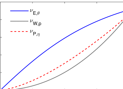
Figure 1: Maximum certificate rates $\gamma_{\textrm{PEF}}$ (Eq. (6)) as a function of $\hat{I}$ for each family of distributions.

For each family of distributions, we determine the maximum certificate rate $\gamma_{\textrm{PEF}}$ as given in Eq. (6). For this, we consider the trial model $\mathcal{N}$, but we note that $\gamma_{\textrm{PEF}}$ does not depend on the specific constraints on the quantum-achievable conditional distributions $\mathbb{P}(AB|XY)$ (see Appendix F). As an indicator of finite-data performance, $\gamma_{\textrm{PEF}}$ depends not only on $\hat{I}$, but also on the distribution $\nu$. To illustrate this behavior, we plot the rates $\gamma_{\textrm{PEF}}$ as a function of $\hat{I}$ for each family of distributions in Fig. 1. To obtain these plots, we note that $\hat{I}$ is a monotonic function of the parameter $\theta$, $p$ or $\eta$ for each family. We also find that $\gamma_{\textrm{PEF}}$ is given by the statistical strength of the distribution $\nu$ for rejecting local realism (see Appendix F for a proof). Conventionally, experiments are designed to maximize $\hat{I}$, but in general, the optimal state and measurements maximizing $\hat{I}$ are different from those maximizing the statistical strength Acín et al. (2005); Zhang et al. (2010).

We further determine the minimum number of trials, $n_{\textrm{PEF},b}$, required to certify $b$ bits of $\epsilon$-smooth conditional min-entropy with a given distribution $\nu$ of trial results. From Eq. (5), we get

$$n_{\textrm{PEF},b}=\inf_{\beta>0}\frac{b\beta-\log_{2}(\epsilon)-(1+\beta)\log_{2}(\kappa)}{\beta g(\beta)},$$

where for simplicity we allow non-integer values for $n_{\textrm{PEF},b}$. We can upper bound $n_{\textrm{PEF},b}$ by means of the simpler-to-compute certificate rate $\gamma_{\textrm{PEF}}$ given in Eq. (6). For the trial model $\mathcal{N}$, $\gamma_{\textrm{PEF}}$ is achieved when $\beta$ is above a threshold $\beta_{0}$ that depends on $\nu$ (see Appendix F). From $\gamma_{\textrm{PEF}}$ and $\beta_{0}$, we can determine the upper bound

$$n^{\prime}_{\textrm{PEF},b}=\big{(}b\beta_{0}-\log_{2}(\epsilon)-(1+\beta_{0})\log_{2}(\kappa)\big{)}/\gamma_{\textrm{PEF}}$$

on $n_{\textrm{PEF},b}$. The minimum number of trials required can be determined for other published protocols, which usually certify conditional min-entropy from $\hat{I}$. (An exception is Ref. Nieto-Silleras et al. (2018) but the minimum number of trials required is worse.) We consider the protocol “PM” of Ref. Pironio and Massar (2013) and the entropy accumulation protocol “EAT” of Ref. Arnon-Friedman et al. (2018). From Thm. 1 of Ref. Pironio and Massar (2013) with $\kappa=1$ and $b\searrow 0$, we obtain a lower bound

$$n_{\textrm{PM},0}=-2\log_{e}(\epsilon)/\big{(}(\hat{I}-2)/(4+2\sqrt{2})\big{)}^{2}.$$

For the EAT protocol, we determine an explicit lower bound $n_{\textrm{EAT},b}$ in Appendix H. This lower bound applies for $b\geq 0$ and $\epsilon,\kappa\in(0,1]$, and is valid with respect to quantum side information for the trial model consisting of quantum-achievable distributions.

We compare the three protocols over a broad range of $\hat{I}$ for $b\searrow 0$, $\epsilon=10^{-6}$, and $\kappa=1$. For each family of distributions above, we compute the improvement factors given by $f_{\textrm{PM}}=n_{\textrm{PM},0}/n^{\prime}_{\textrm{PEF},0}$ and $f_{\textrm{EAT}}=n_{\textrm{EAT},0}/n^{\prime}_{\textrm{PEF},0}$. For $\nu_{\textrm{W},p}$, the improvement factors depend weakly on $\hat{I}$: $f_{\textrm{PM}}$ increases from $3.89$ at $\hat{I}=2.008$ to $4.36$ at $\hat{I}=2\sqrt{2}$, while $f_{\textrm{EAT}}$ increases from $84.97$ at $\hat{I}=2.008$ to $86.35$ at $\hat{I}=2\sqrt{2}$. For $\nu_{\textrm{E},\theta}$ and $\nu_{\textrm{P},\eta}$, the improvement factors can be much larger and depend strongly on $\hat{I}$, monotonically decreasing with $\hat{I}$ as shown in Fig. 2. The improvement is particularly notable at small violations which are typical in current photonic loophole-free Bell tests. We remark that similar comparison results were obtained with other choices of the values for $\epsilon$ and $\kappa$.

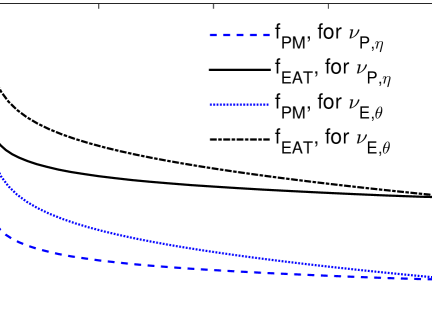
Figure 2: Improvement factors as a function of $\hat{I}$.

The large latency reduction with probability estimation persists for certifying blocks of randomness. For randomness beacons, good reference values are $b=512$ and $\epsilon=2^{-64}$. We also set $\kappa=2^{-64}$. Setting $\kappa=\epsilon$ is a common conservative choice, but we remark that soundness for randomness generation can be defined with a better tradeoff between $\epsilon$ and $\kappa$ Knill et al. (2017). We consider the trial model $\mathcal{T}$ of distributions with uniformly random inputs, satisfying both non-signaling conditions Popescu and Rohrlich (1994) and Tsirelson’s bounds Cirelśon (1980). Consider the state-of-the-art photonic loophole-free Bell test reported in Ref. Bierhorst et al. (2018). With probability estimation, the number of trials required for the distribution inferred from the measurement statistics is $4.668\times 10^{7}$, which would require about $7.78$ minutes of running time in the referenced experiment. With entropy accumulation Arnon-Friedman et al. (2018), $2.887\times 10^{11}$ trials taking $802$ hours would be required. For atomic experiments, we can use the distribution inferred from the measurement statistics in Ref. Rosenfeld et al. (2017), for which probability estimation requires $7.354\times 10^{4}$ trials, while entropy accumulation Arnon-Friedman et al. (2018) requires $5.629\times 10^{6}$. The experiment of Ref. Rosenfeld et al. (2017) observed $1$ to $2$ trials per minute, so probability estimation would have needed at least $612.8$ hours of data collection, which while impractical is still less than the $5.35$ years required by entropy accumulation Arnon-Friedman et al. (2018).

Finally, we briefly discuss the performance of probability estimation on DIRG with published Bell-test experimental data. The first experimental demonstration of conditional min-entropy certification for DIRG is reported in Ref. Pironio et al. (2010). The method therein certifies the presence of $42$ random bits at error bound $\epsilon=10^{-2}$ against classical side information, where the trial model consists of quantum-achievable distributions with uniform inputs. (The lower bound of the protocol success probability $\kappa=1$ was used implicitly in Ref. Pironio et al. (2010), so $\kappa=1$ in the following comparison.) For the same data but with the less restrictive trial model $\mathcal{T}$, probability estimation certifies the presence of at least nine times more random bits with $\epsilon=10^{-2}$. With $\epsilon=10^{-6}$ probability estimation can still certify the presence of $80$ random bits, while other methods fail to certify any random bits. For the loophole-free Bell-test data reported in Ref. Shalm et al. (2015) and analyzed in our previous work Ref. Bierhorst et al. (2017), the presence of $894$ random bits at $\epsilon=10^{-3}$ was certified against classical side information with the trial model $\mathcal{N}$. Further, $256$ private random bits within $10^{-3}$ (in terms of the total-variation distance) of uniform were extracted in Ref. Bierhorst et al. (2017). With probability estimation we can certify the presence of approximately two times more random bits at $\epsilon=10^{-3}$. The presence of four times more bits can be certified if we use the more restrictive trial model $\mathcal{T}$. Furthermore, we can certify randomness even when the input distribution is not precisely known, which was an issue in the experiment of Ref. Shalm et al. (2015). Applications to other experimental distributions, complete analyses of the mentioned experiments, and details on handling input choices whose probabilities are not precisely known are in Ref. Knill et al. (2017).

In conclusion, probability estimation is a powerful and flexible framework for certifying randomness in data from a finite sequence of experimental trials. Implemented with probability estimation factors, it witnesses optimal asymptotic randomness rates. For practical applications requiring fixed-size blocks of random bits, it can reduce the latencies by orders of magnitude even for high-quality devices. Latency is a notable problem for device-independent quantum key generation (DIQKD). If probability estimation can be extended to accommodate security against quantum side information, the latency reductions may be extendable to DIQKD by means of existing constructions Arnon-Friedman et al. (2018).

Finally we remark that if the trial results are explainable by local realism, no device-independent randomness would be certified by probability estimation. The reason is as follows. For simplicity we assume that the input distribution is fixed and known . Consider a generic trial with results $CZ$ and model $\mathcal{C}$. Let $\mathcal{P}_{\text{LR}}$ be the set of distributions of $CZ$ explainable by local realism, which is a convex polytope with a finite number of extremal distributions $\sigma_{\text{LR},k}$, $k=1,2,...,K$. Since $\mathcal{P}_{\text{LR}}$ is a subset of $\mathcal{C}$, by definition a PEF $F$ with power $\beta$ satisfies the condition

$$\sum_{cz}F(cz)\sigma_{\text{LR},k}(c|z)^{\beta}\sigma_{\text{LR},k}(cz)\leq 1,$$ (7)

for each $k$. For each extremal distribution $\sigma_{\text{LR},k}$ in $\mathcal{P}_{\text{LR}}$ and each $cz$, the value of $\sigma_{\text{LR},k}(c|z)$ is either $0$ or $1$, from which it follows that $\sigma_{\text{LR},k}(c|z)^{\beta}\sigma_{\text{LR},k}(cz)=\sigma_{\text{LR},k}(cz)$. Eq. (7) now becomes

$$\mathbb{E}_{\sigma_{\text{LR},k}}\big{(}F(CZ)\big{)}=\sum_{cz}F(cz)\sigma_{\text{LR},k}(cz)\leq 1.$$ (8)

Since any local realistic distribution can be written as a convex mixture of extremal distributions $\sigma_{\text{LR},k}$, $k=1,2,...,K$, Eq. (8) implies that for all distributions $\nu\in\mathcal{P}_{\text{LR}}$

$$\mathbb{E}_{\nu}\big{(}F(CZ)\big{)}\leq 1.$$ (9)

By the concavity of the logarithm function and Eq. (9) we get that

$$\mathbb{E}_{\nu}\big{(}\log_{2}(F(CZ))\big{)}\leq\log_{2}\big{(}\mathbb{E}_{\nu}(F(CZ))\big{)}\leq 0.$$

Hence, the asymptotic entropy rate in Eq. (4) cannot be positive if the distribution of trial results is explainable by local realism. Furthermore, Eq. (9) shows that the PEF $F$ is a test factor for the hypothesis test of local realism Zhang et al. (2011) (see Appendix B for the formal definition of test factors). So, if a finite sequence of trial results is explainable by local realism and $F_{i}$ is a PEF with power $\beta$ for the $i$’th trial, according to Ref. Zhang et al. (2011) the success event $T_{n}\geq 1/(p^{\beta}\epsilon)$ with $T_{n}=\prod_{i=1}^{n}F_{i}$ in Thm. 1 for randomness certification would happen with probability at most $p^{\beta}\epsilon$.

Appendix

Appendix A Notation

Much of this work concerns stochastic sequences, that is, sequences of random variables (RVs). RVs are functions on an underlying probability space. The range of an RV is called its value space and may be thought of as the set of its observable values or realizations. Here, all RVs have countable value spaces. We truncate sequences of RVs so that we only consider finitely many RVs at a time. With this the underlying probability space is countable too. We use upper-case letters such as $A,B,\ldots,X,Y,\ldots$ to denote RVs. The value space of an RV such as $X$ is denoted by $\mathrm{Rng}(X)$. The cardinality of the value space of $X$ is $|\mathrm{Rng}(X)|$. Values of RVs are denoted by the corresponding lower-case letters. Thus $x$ is a value of $X$, often thought of as the particular value realized in an experiment. When using symbols for values of RVs, they are implicitly assumed to be members of the range of the corresponding RV. In many cases, the value space is a set of letters or a set of strings of a given length. We use juxtaposition to denote concatenation of letters and strings. Stochastic sequences are denoted by capital bold-face letters, with the corresponding lower-case bold-face letters for their values. For example, we write $\mathbf{A}=(A_{i})_{i=1}^{N}$ and $\mathbf{A}_{\leq m}=(A_{i})_{i=1}^{m}$. Our conventions for indices are that we generically use $N$ to denote a large upper bound on sequence lengths, $n$ to denote the available length and $i,j,k,l,m$ as running indices. By convention, $\mathbf{A}_{\leq 0}$ is the empty sequence of RVs. Its value is constant. When multiple stochastic sequences are in play, we refer to the collection of $i$’th RVs in the sequences as the data from the $i$’th trial. We typically imagine the trials as happening in time and being performed by an experimenter. We refer to the data from the trials preceding the upcoming one as the “past”. The past can also include initial conditions and any additional information that may have been obtained. These are normally implicit when referring to or conditioning on the past.

Probabilities are denoted by $\mathbb{P}(\ldots)$. If there are multiple probability distributions involved, we disambiguate with a subscript such as in $\mathbb{P}_{\nu}(\ldots)$ or simply $\nu(\ldots)$, where $\nu$ is a probability distribution. We generally reserve the symbol $\mu$ for the global, implicit probability distribution, and may write $\mu(\ldots)$ instead of $\mathbb{P}(\ldots)$ or $\mathbb{P}_{\mu}(\ldots)$. Expectations are similarly denoted by $\mathbb{E}(\ldots)$ or $\mathbb{E}_{\mu}(\ldots)$. If $\phi$ is a logical expression involving RVs, then $\{\phi\}$ denotes the event where $\phi$ is true for the values realized by the RVs. For example, $\{f(X)>0\}$ is the event $\{x:f(x)>0\}$ written in full set notation. The brackets $\{\ldots\}$ are omitted for events inside $\mathbb{P}(\ldots)$ or $\mathbb{E}(\ldots)$. As is conventional, commas separating logical expressions are interpreted as conjunction. When the capital/lower-case convention can be unambiguously interpreted, we abbreviate “$X=x$” as “$x$”. For example, with this convention, $\mathbb{P}(x,y)=\mathbb{P}(X=x,Y=y)$. Furthermore, we omit commas in the abbreviated notation, so $\mathbb{P}(xy)=\mathbb{P}(x,y)$. RVs or functions of RVs appearing outside an event but inside $\mathbb{P}(\ldots)$ or after the conditioner in $\mathbb{E}(\ldots|\ldots)$ result in an expression that is itself an RV. We can define these without complications because of our assumption that the event space is countable. Here are two examples. $\mathbb{P}(f(X)|Y)$ is a function of the RVs $X$ and $Y$ and can be described as the RV whose value is $\mathbb{P}(f(X)=f(x)|Y=y)$ whenever the values of $X$ and $Y$ are $x$ and $y$, respectively. Similarly $\mathbb{E}(X|Y)$ is the RV defined as a function of $Y$, with value $\mathbb{E}(X|Y=y)$ whenever $Y$ has value $y$. Note that $X$ plays a different role before the conditioners in $\mathbb{E}(\ldots)$ than it does in $\mathbb{P}(\ldots)$, as $\mathbb{E}(X|Y)$ is not a function of $X$, but only of $Y$. We comment that conditional probabilities with conditioners having probability zero are not well-defined, but in most cases can be defined arbitrarily. Typically, they occur in a context where they are multiplied by the probability of the conditioner and thereby contribute zero regardless. An important context involves expectations, where we use the convention that when expanding an expectation over a set of values as a sum, zero-probability values are omitted. We do so without explicitly adding the constraints to the summation variables. We generally use conditional probabilities without explicitly checking for probability-zero conditioners, but it is necessary to monitor for well-definedness of the expressions obtained.

To denote general probability distributions, usually on the joint value spaces of RVs, we use symbols such as $\mu,\nu,\sigma$, with modifiers as necessary. As mentioned, we reserve the unmodified $\mu$ for the distinguished global distribution under consideration, if there is one. Other symbols typically refer to probability distributions defined on the joint range of a subset of the available RVs. We usually just say “distribution” instead of “probability distribution”. The terms “distributions on $\mathrm{Rng}(X)$” and “distributions of $X$” are synonymous. If $\nu$ is a joint distribution of RVs, then we extend the conventions for arguments of $\mathbb{P}(\ldots)$ to arguments of $\nu$, as long as all the arguments are determined by the RVs for which $\nu$ is defined. For example, if $\nu$ is a joint distribution of $X$, $Y$, and $Z$, then $\nu(x|y)$ has the expected meaning, as does the RV $\nu(X|Y)$ in contexts requiring no other RVs. Further, $\nu(X)$ and $\nu(XY)$ are the marginal distributions of $X$ and $XY$, respectively, according to $\nu$.

In our work, probability distributions are constrained by a “model”, which is defined as a set of distributions and denoted by letters such as $\mathcal{H}$ or $\mathcal{C}$. The models for trials to be considered here are usually convex and closed.

The total-variation (TV) distance between $\nu$ and $\nu^{\prime}$ is defined as

$$\mathrm{TV}(\nu,\nu^{\prime})=\sum_{x}(\nu(x)-\nu^{\prime}(x))\left\llbracket\nu(x)\geq\nu^{\prime}(x)\right\rrbracket=\frac{1}{2}\sum_{x}|\nu(x)-\nu^{\prime}(x)|,$$ (10)

where $\left\llbracket\phi\right\rrbracket$ for a logical expression $\phi$ denotes the $\{0,1\}$-valued function evaluating to $1$ iff $\phi$ is true. True to its name, the TV distance satisfies the triangle inequality. Here are three other useful properties: First, if $\nu$ and $\nu^{\prime}$ are joint distributions of $X$ and $Y$ and the marginals satisfy $\nu(Y)=\nu^{\prime}(Y)$, then the TV distance between $\nu$ and $\nu^{\prime}$ is the average of the TV distances of the $Y$-conditional distributions:

$$\mathrm{TV}(\nu,\nu^{\prime})=\sum_{y}\nu(y)\mathrm{TV}(\nu(X|y),\nu^{\prime}(X|y)).$$ (11)

Second, if for all $y$, the conditional distributions $\nu(X|y)=\nu^{\prime}(X|y)$, then the TV distance between $\nu$ and $\nu^{\prime}$ is given by the TV distance between the marginals on $Y$:

$$\mathrm{TV}(\nu,\nu^{\prime})=\mathrm{TV}(\nu(Y),\nu^{\prime}(Y)).$$ (12)

Third, the TV distance satisfies the data-processing inequality. That is, for any stochastic process $\mathcal{E}$ on $\mathrm{Rng}(X)$ and distributions $\nu$ and $\nu^{\prime}$ of $X$, $\mathrm{TV}(\mathcal{E}(\nu),\mathcal{E}(\nu^{\prime}))\leq\mathrm{TV}(\nu,\nu^{\prime})$. We use this property only for functions $\mathcal{E}$, but for general forms of this result, see Ref. Pardo and Vajda (1997). The above properties of TV distances are well known, specific proofs can be found in Refs. Knill et al. (2017); Bierhorst et al. (2018).

When constructing distributions close to a given one in TV distance, which we need to do for the proof of Thm. 1 in the main text, it is often convenient to work with subprobability distributions. A subprobability distribution of $X$ is a sub-normalized non-negative measure on $\mathrm{Rng}(X)$, which in our case is simply a non-negative function $\tilde{\nu}$ on $\mathrm{Rng}(X)$ with weight $w(\tilde{\nu})=\sum_{x}\tilde{\nu}(x)\leq 1$. For expressions not involving conditionals, we use the same conventions for subprobability distributions as for probability distributions. When comparing subprobability distributions, $\tilde{\nu}\leq\tilde{\nu}^{\prime}$ means that for all $x$, $\tilde{\nu}(x)\leq\tilde{\nu}^{\prime}(x)$, and we say that $\tilde{\nu}^{\prime}$ “dominates” $\tilde{\nu}$.

Lemma 2.

Let $\tilde{\nu}$ be a subprobability distribution of $X$ of weight $w=1-\epsilon$. Let $\nu$ and $\nu^{\prime}$ be distributions of $X$ satisfying $\tilde{\nu}\leq\nu$ and $\tilde{\nu}\leq\nu^{\prime}$. Then $\mathrm{TV}(\nu,\nu^{\prime})\leq\epsilon$.

Proof.

Calculate

$$\mathrm{TV}(\nu,\nu^{\prime}) =\sum_{x}(\nu(x)-\nu^{\prime}(x))\left\llbracket\nu(x)\geq\nu^{\prime}(x)\right\rrbracket$$

$$\leq\sum_{x}(\nu(x)-\tilde{\nu}(x))\left\llbracket\nu(x)\geq\tilde{\nu}(x)\right\rrbracket$$

$$=\sum_{x}(\nu(x)-\tilde{\nu}(x))$$

$$=1-w=\epsilon.$$

∎

Lemma 3.

Assume that $p\geq 1/|\mathrm{Rng}(X)|$. Let $\nu$ be a distribution of $X$ and $\tilde{\nu}\leq\nu$ a subprobability distribution of $X$ with weight $w=1-\epsilon$ and $\tilde{\nu}\leq p$. Then there exists a distribution $\nu^{\prime}$ of $X$ with $\nu^{\prime}\geq\tilde{\nu}$, $\nu^{\prime}\leq p$, and $\mathrm{TV}(\nu,\nu^{\prime})\leq\epsilon$.

Proof.

Because $p\geq 1/|\mathrm{Rng}(X)|$, that is, $\sum_{x}p\geq 1$, and for all $x$, $\tilde{\nu}(x)\leq p$, there exists a distribution $\nu^{\prime}\geq\tilde{\nu}$ with $\nu^{\prime}\leq p$. Since $\nu^{\prime}$ and $\nu$ are distributions dominating $\tilde{\nu}$ and by Lem. 2, $\mathrm{TV}(\nu,\nu^{\prime})\leq\epsilon$. ∎

Appendix B Test Supermartingales and Test Factors

Definition 4.

A test supermartingale Shafer et al. (2011) with respect to a stochastic sequence $\mathbf{R}$ and model $\mathcal{H}$ is a stochastic sequence $\mathbf{T}=(T_{i})_{i=0}^{N}$ with the properties that 1) $T_{0}=1$, 2) for all $i$ $T_{i}\geq 0$, 3) $T_{i}$ is determined by $\mathbf{R}_{\leq i}$ and the governing distribution, and 4) for all distributions in $\mathcal{H}$, $\mathbb{E}(T_{i+1}|\mathbf{R}_{\leq i})\leq T_{i}$. The ratios $F_{i}=T_{i}/T_{i-1}$ with $F_{i}=1$ if $T_{i-1}=0$ are called the test factors of $\mathbf{T}$.

Here $\mathbf{R}$ captures the relevant information that accumulates in a sequence of trials. It does not need to be accessible to the experimenter. Between trials $i$ and $i+1$, the sequence $\mathbf{R}_{\leq i}$ is called the past. In the definition, we allow for $T_{i}$ to depend on the governing distribution $\mu$. With this, for a given $\mu$, $T_{i}$ is a function of $\mathbf{R}_{\leq i}$. Below, when stating that RVs are determined, we implicitly include the possibility of dependence on $\mu$ without mention. The $\mu$-dependence can arise through expressions such as $\mathbb{E}_{\mu}(G|\mathbf{R}_{\leq i})$ for some $G$, which is determined by $\mathbf{R}_{\leq i}$ given $\mu$. One way to formalize this is to consider $\mu$-parameterized families of RVs. We do not make this explicit and simply allow for our RVs to be implicitly parameterized by $\mu$. We note that the governing distribution in a given experiment or situation is fixed but usually unknown with most of its features inaccessible. As a result, many RVs used in mathematical arguments cannot be observed even in principle. Nevertheless, they play important roles in establishing relationships between observed and inferred quantities.

Defining $F_{i}=1$ when $T_{i-1}=0$ makes sense because given $\{T_{i-1}=0\}$, we have $\{T_{i}=0\}$ with probability $1$. The sequence $\mathbf{F}=(F_{i})_{i=1}^{N}$ satisfies the conditions that for all $i$, 1) $F_{i}\geq 0$, 2) $F_{i}$ is determined by $\mathbf{R}_{\leq i}$, and 3) for all distributions in $\mathcal{H}$, $\mathbb{E}(F_{i+1}|\mathbf{R}_{\leq i})\leq 1$. We can define test supermartingales in terms of such sequences: Let $\mathbf{F}$ be a stochastic sequence satisfying the three conditions. Then the stochastic sequence with members $T_{0}=1$ and $T_{i}=\prod_{1\leq j\leq i}F_{j}$ for $i\geq 1$ is a test supermartingale. It suffices to check that $\mathbb{E}(T_{i+1}|\mathbf{R}_{\leq i})\leq T_{i}$. This follows from

$$\mathbb{E}(T_{i+1}|\mathbf{R}_{\leq i})=\mathbb{E}(F_{i+1}T_{i}|\mathbf{R}_{\leq i})=\mathbb{E}(F_{i+1}|\mathbf{R}_{\leq i})T_{i}\leq T_{i},$$

where we pulled out the determined quantity $T_{i}$ from the conditional expectation. In this work, we construct test supermartingales from sequences $\mathbf{F}$ with the above properties. We refer to any such sequence as a sequence of test factors, without necessarily making the associated test supermartingale explicit. We extend the terminology by calling an RV $F$ a test factor with respect to $\mathcal{H}$ if $F\geq 0$ and $\mathbb{E}(F)\leq 1$ for all distributions in $\mathcal{H}$. Note that $F=1$ is a valid test factor.

For an overview of test supermartingales and their properties, see Ref. Shafer et al. (2011). The notion of test supermartingales and proofs of their basic properties are due to Ville Ville (1939) in the same work that introduced the notion of martingales. The name “test supermartingale” appears to have been introduced in Ref. Shafer et al. (2011). Test supermartingales play an important theoretical role in proving many results in martingale theory, including that of proving tail bounds for large classes of martingales. They have been studied and applied to Bell tests Zhang et al. (2011, 2013); Christensen et al. (2015).

The definition implies that for a test supermartingale $\mathbf{T}$, for all $n$, $\mathbb{E}(T_{n})\leq 1$. This follows inductively from $\mathbb{E}(T_{i+1})=\mathbb{E}(\mathbb{E}(T_{i+1}|\mathbf{R}_{\leq i}))\leq\mathbb{E}(T_{i})$ and $T_{0}=1$. An application of Markov’s inequality shows that for all $\epsilon>0$,

$$\mathbb{P}(T_{n}\geq 1/\epsilon)\leq\epsilon.$$ (13)

Thus, a large final value $t=T_{n}$ of the test supermartingale is evidence against $\mathcal{H}$ in a hypothesis test with $\mathcal{H}$ as the (composite) null hypothesis. Specifically, the RV $1/T$ is a $p$-value bound against $\mathcal{H}$, where in general, the RV $U$ is a $p$-value bound against $\mathcal{H}$ if for all distributions in $\mathcal{H}$, $\mathbb{P}(U\leq\epsilon)\leq\epsilon$.

One can produce a test supermartingale adaptively by determining the test factors $F_{i+1}$ to be used at the next trial. If the $i$’th trial’s data is $R_{i}$, including any incidental information obtained, then $F_{i+1}$ is expressed as a function of $\mathbf{R}_{\leq i}$ and data from the $(i+1)$’th trial (a “past-parameterized” function of $R_{i+1}$), and constructed to satisfy $F_{i+1}\geq 0$ and $\mathbb{E}(F_{i+1}|\mathbf{R}_{\leq i})\leq 1$ for any distribution in the model $\mathcal{H}$. Note that inbetween trials, we can effectively stop the experiment by assigning all future $F_{i+1}=1$, which is a valid test factor, conditional on the past. This is equivalent to constructing the stopped process relative to a stopping rule. This argument also shows that the stopped process is still a test supermartingale.

More generally, we use test supermartingales for estimating lower bounds on products of positive stochastic sequences $\mathbf{G}$. Such lower bounds are associated with unbounded-above confidence intervals. We need the following definition:

Definition 5.

Let $U,V,X$ be RVs and $1\geq\epsilon\geq 0$. $I=[U,V]$ is a confidence interval for $X$ at level $\epsilon$ with respect to $\mathcal{H}$ if for all distributions in $\mathcal{H}$ we have $\mathbb{P}(U\leq X\leq V)\geq 1-\epsilon$. The quantity $\mathbb{P}(U\leq X\leq V)$ is called the coverage probability.

As noted above, the RVs $U$, $V$ and $X$ may be $\mu$-dependent. For textbook examples of confidence intervals such as in Ch. 2.4.3 of Ref Shao (2003), $X$ is a parameter determined by $\mu$, and $U$ and $V$ are obtained according to a known distribution for an estimator of $X$. The quantity $\epsilon$ in the definition is a significance level, which corresponds to a confidence level of $(1-\epsilon)$. The following technical lemma will be used in the next section.

Lemma 6.

Let $\mathbf{F}$ and $\mathbf{G}$ be two stochastic sequences with $F_{i}\in[0,\infty)$, $G_{i}\in(0,\infty]$, and $F_{i}$ and $G_{i}$ determined by $\mathbf{R}_{\leq i}$. Define $T_{0}=1$, $T_{i}=\prod_{1\leq j\leq i}F_{i}$ and $U_{0}=1$, $U_{i}=\prod_{1\leq j\leq i}G_{i}$, and suppose that for all $\mu\in\mathcal{H}$, $\mathbb{E}(F_{i+1}/G_{i+1}|\mathbf{R}_{\leq i})\leq 1$. Then $[T_{n}\epsilon,\infty)$ is a confidence interval for $U_{n}$ at level $\epsilon$ with respect to $\mathcal{H}$.

Proof.

The assumptions imply that the sequence $(F_{i}/G_{i})_{i=1}^{N}$ forms a sequence of test factors with respect to $\mathcal{H}$ and generate the test supermartingale $\mathbf{T}/\mathbf{U}$, where division in this expression is term-by-term. Therefore, by Eq. (13),

$$\mathbb{P}(T_{n}\epsilon\geq U_{n})=\mathbb{P}(T_{n}/U_{n}\geq 1/\epsilon)\leq\epsilon,$$ (14)

so $[T_{n}\epsilon,\infty)$ is a confidence interval for $U_{n}$ at level $\epsilon$. ∎

Appendix C Proof of Main Results

In this section, we show how to perform probability estimation and how to certify smooth conditional min-entropy by probability estimation.

C.1 Probability Estimation by Test Supermartingales: Proof of Main Text Eq. (1)

We consider the situation where $\mathbf{CZ}$ is a time-ordered sequence of $n$ trial results, and the classical side information is represented by an RV $E$ with countable value space. In an experiment, $\mathbf{Z}$ and $\mathbf{C}$ are the inputs and outputs of the quantum devices, and the side information $E$ is carried by an external classical system E. Before the experiment, the initial state of E may be correlated with the quantum devices. At each trial of the experiment, we allow arbitrary one-way communication from the system E to the devices. For example, E can initialize the state of the quantum devices via a one-way communication channel. We also allow the possibility that the device initialization at a trial by E depends on the past inputs preceding the trial. This implies that the random inputs $\mathbf{Z}$ can come from public-randomness sources, as first pointed out in Ref. Pironio and Massar (2013). However, at any stage of the experiment the information of the outputs $\mathbf{C}$ cannot be leaked to the system E. After the experiment, we observe $\mathbf{Z}$ and $\mathbf{C}$, but not the side information $E$.

A model $\mathcal{H}$ for an experiment is defined as the set of joint probability distributions of $\mathbf{CZ}$ that satisfy the known constraints and consists of all achievable probability distributions of $\mathbf{CZ}$ conditional on values $e$ of $E$. Thus we say that a joint distribution $\mu$ of $\mathbf{CZ}$ and $E$ satisfies the model $\mathcal{H}$ if $\mu(\mathbf{C}\mathbf{Z}|E=e)\in\mathcal{H}$ for each value $e$.

We focus on probability estimates with lower bounds on coverage probabilities that do not depend on $E$. Our specific goal is to prove Eq. (1) in the main text. We will show that the probability bound of $U(\mathbf{CZ})=(T_{n}\epsilon)^{-1/\beta}$ in Eq. (1) of the main text is an instance of what we call an “$\epsilon$-uniform probability estimator”:

Definition 7.

Let $1\geq\epsilon\geq 0$. The function $U:\mathrm{Rng}(\mathbf{CZ})\rightarrow[0,\infty)$ is a level-$\epsilon$ $E$-uniform probability estimator for $\mathcal{H}$ ($\epsilon$-$\mathrm{UPE}$ or with specifics, $\epsilon$-$\mathrm{UPE}(\mathbf{C}|\mathbf{Z}E;\mathcal{H})$) if for all $e$ and distributions $\mu$ satisfying the model $\mathcal{H}$, we have $\mathbb{P}_{\mu}(U(\mathbf{CZ})\geq\mu(\mathbf{C}|\mathbf{Z}e)|e)\geq 1-\epsilon$. We omit specifics such as $\mathcal{H}$ if they are clear from context.

We can obtain $\epsilon$-$\mathrm{UPE}$s by constructing test supermartingales. In order to achieve this goal, we consider models $\mathcal{H}(\mathcal{C})$ of distributions of $\mathbf{CZ}$ constructed from a chain of trial models $\mathcal{C}_{i+1|\mathbf{c}_{\leq i}\mathbf{z}_{\leq i}e}$, where the trial model $\mathcal{C}_{i+1|\mathbf{c}_{\leq i}\mathbf{z}_{\leq i}e}$ is defined as the set of all achievable distributions of $C_{i+1}Z_{i+1}$ conditional on both the past results $\mathbf{c}_{\leq i}\mathbf{z}_{\leq i}$ and the value $e$ of $E$. The chained model $\mathcal{H}(\mathcal{C})$ consists of all conditional distributions $\mu(\mathbf{C}\mathbf{Z}|e)$ satisfying the following two properties. First, for all $i$, $\mathbf{c}_{\leq i}\mathbf{z}_{\leq i}$, and $e$, the conditional distributions

$$\mu(C_{i+1}Z_{i+1}|\mathbf{c}_{\leq i}\mathbf{z}_{\leq i}e)\in\mathcal{C}_{i+1|\mathbf{c}_{\leq i}\mathbf{z}_{\leq i}e}.$$

Second, the joint distribution $\mu$ of $\mathbf{CZ}$ and $E$ satisfies that $Z_{i+1}$ is independent of $\mathbf{C}_{\leq i}$ conditionally on both $\mathbf{Z}_{\leq i}$ and $E$. The second condition is needed in order to be able to estimate $\mathbf{Z}E$-conditional probabilities of $\mathbf{C}$ and corresponds to the Markov-chain condition in the entropy accumulation framework Arnon-Friedman et al. (2018).

In many cases, the trial models $\mathcal{C}_{i+1|\mathbf{c}_{\leq i}\mathbf{z}_{\leq i}e}$ do not depend on the past outputs $\mathbf{c}_{\leq i}$, but probability estimation can take advantage of dependence on the past inputs $\mathbf{z}_{\leq i}$. Such dependence captures the possibility that at the $(i+1)$’th trial the device initialization by the external classical system E depends on the past inputs $\mathbf{z}_{\leq i}$. In applications involving Bell-test configurations, the trial models capture constraints on the input distributions and on non-signaling or quantum behavior of the devices. For simplicity, we write $\mathcal{C}_{i+1}=\mathcal{C}_{i+1|\mathbf{c}_{\leq i}\mathbf{z}_{\leq i}e}$, leaving the conditional parameters implicit. Normally, models for individual trials $\mathcal{C}_{i+1}$ are convex and closed. If they are not, we note that our results generally extend to the convex closures of the trial models used.

For chained models $\mathcal{H}(\mathcal{C})$, we can construct $\epsilon$-$\mathrm{UPE}$s from products of “probability estimation factors” according to the following definition, see also the paragraph containing Eq. (1) in the main text.

Definition 8.

Let $\beta>0$, and let $\mathcal{C}$ be any model, not necessarily convex. A probability estimation factor (PEF) with power $\beta$ for $\mathcal{C}$ is a non-negative RV $F=F(CZ)$ such that for all $\sigma\in\mathcal{C}$, $\mathbb{E}_{\sigma}(F\sigma(C|Z)^{\beta})\leq 1$.

We emphasize that a PEF is a function of the trial results $CZ$, but not of the side information $E$.

Consider the model $\mathcal{H}(\mathcal{C})$ constructed as a chain of trial models $\mathcal{C}_{i}$. Let $F_{i}$ be PEFs with power $\beta>0$ for $\mathcal{C}_{i}$, past-parameterized by $\mathbf{C}_{<i}$ and $\mathbf{Z}_{<i}$. Define $T_{0}=1$, $T_{i}=\prod_{1\leq j\leq i}F_{j}$ for $i\geq 1$, and

$$U(\mathbf{CZ})=(T_{n}\epsilon)^{-1/\beta}.$$ (15)

Then, $U(\mathbf{CZ})$ satisfies the inequality in Eq. (1) of the main text as proven in the following theorem, and is therefore an $\epsilon$-$\mathrm{UPE}$. To simplify notation in the following theorem, we normally write the distribution $\mu(\mathbf{C}\mathbf{Z}|e)$ conditional on $e$ as $\mu_{e}(\mathbf{C}\mathbf{Z})$, abbreviated as $\mu_{e}$.

Theorem 9.

Fix $\beta>0$. For each value $e$ of $E$, each $\mu_{e}\in\mathcal{H}(\mathcal{C})$, and $\epsilon>0$, the following inequality holds:

$$\mathbb{P}_{\mu_{e}}\big{(}\mu_{e}(\mathbf{C}|\mathbf{Z})\geq(\epsilon T_{n})^{-1/\beta}\big{)}\leq\epsilon.$$ (16)

Note that $\beta$ cannot be adapted during the trials. On the other hand, before the $i$’th trial, we can design the PEFs $F_{i}$ for the particular constraints relevant to the $i$’th trial.

Proof.

We first observe that for each value $e$ of $E$,

$$\prod_{j=0}^{i-1}\mu_{e}(C_{j+1}|Z_{j+1}\mathbf{Z}_{\leq j}\mathbf{C}_{\leq j})=\mu_{e}(\mathbf{C}_{\leq i}|\mathbf{Z}_{\leq i}).$$ (17)

This follows by induction with the identity

$$\mu_{e}(\mathbf{C}_{\leq j+1}|\mathbf{Z}_{\leq j+1}) =\mu_{e}(C_{j+1}|Z_{j+1}\mathbf{Z}_{\leq j}\mathbf{C}_{\leq j})\mu_{e}(\mathbf{C}_{\leq j}|Z_{j+1}\mathbf{Z}_{\leq j})$$

$$=\mu_{e}(C_{j+1}|Z_{j+1}\mathbf{Z}_{\leq j}\mathbf{C}_{\leq j})\mu_{e}(\mathbf{C}_{\leq j}|\mathbf{Z}_{\leq j})$$

by conditional independence of $Z_{j+1}$ on $\mathbf{C}_{\leq j}$ given $\mathbf{Z}_{\leq j}$ and $E=e$.

We claim that for each $e$, $F_{i+1}\mu_{e}(C_{i+1}|Z_{i+1}\mathbf{Z}_{\leq i}\mathbf{C}_{\leq i})^{\beta}$ is a test factor determined by $\mathbf{C}_{\leq i+1}\mathbf{Z}_{\leq i+1}$. To prove this claim, for all $\mathbf{c}_{\leq i}\mathbf{z}_{\leq i}$, the distributions $\nu=\mu_{e}(C_{i+1}Z_{i+1}|\mathbf{c}_{\leq i}\mathbf{z}_{\leq i})\in\mathcal{C}_{i+1}$. With $F_{i+1}=F_{i+1}(C_{i+1}Z_{i+1};\mathbf{c}_{\leq i}\mathbf{z}_{\leq i})$, we obtain the bound

$$\mathbb{E}\left(F_{i+1}\mu_{e}(C_{i+1}|Z_{i+1}\mathbf{z}_{\leq i}\mathbf{c}_{\leq i})^{\beta}|\mathbf{c}_{\leq i}\mathbf{z}_{\leq i}\right) =\mathbb{E}_{\nu}\left(F_{i+1}\nu(C_{i+1}|Z_{i+1})^{\beta}\right)$$

$$\leq 1,$$

where we invoked the assumption that $F_{i+1}$ is a PEF with power $\beta$ for $\mathcal{C}_{i+1}$. By arbitrariness of $\mathbf{c}_{\leq i}\mathbf{z}_{\leq i}$, and because the factors $F_{i+1}\mu_{e}(C_{i+1}|Z_{i+1}\mathbf{Z}_{\leq i}\mathbf{C}_{\leq i})^{\beta}$ are determined by $\mathbf{C}_{\leq i+1}\mathbf{Z}_{\leq i+1}$, the claim follows. The product of these test factors is

$$\prod_{j=0}^{i-1}F_{j+1}\mu_{e}(C_{j+1}|Z_{j+1}\mathbf{Z}_{\leq j}\mathbf{C}_{\leq j})^{\beta} =T_{i}\prod_{j=0}^{i-1}\mu_{e}(C_{j+1}|Z_{j+1}\mathbf{Z}_{\leq j}\mathbf{C}_{\leq j})^{\beta}$$

$$=T_{i}\mu_{e}(\mathbf{C}_{\leq i}|\mathbf{Z}_{\leq i})^{\beta},$$ (18)

with $T_{i}=\prod_{j=1}^{i}F_{j}$. To obtain the last equality above, we used Eq. (17). Thus, for each $e$, the sequence $Q_{0}=1$ and $Q_{i}=T_{i}\mu_{e}(\mathbf{C}_{\leq i}|\mathbf{Z}_{\leq i})^{\beta}$ for $i>0$ satisfies the supermartingale property $\mathbb{E}_{\mu_{e}}(Q_{i+1}|\mathbf{C}_{\leq i}\mathbf{Z}_{\leq i})\leq Q_{i}$. We remark that as a consequence, $\mathbb{E}_{\mu_{e}}(Q_{i+1})=\mathbb{E}_{\mu_{e}}\big{(}\mathbb{E}_{\mu_{e}}(Q_{i+1}|\mathbf{C}_{\leq i}\mathbf{Z}_{\leq i})\big{)}\leq\mathbb{E}_{\mu_{e}}(Q_{i})$. By induction this gives $\mathbb{E}_{\mu_{e}}(Q_{n})=\mathbb{E}_{\mu_{e}}(T_{n}\mu_{e}(\mathbf{C}|\mathbf{Z})^{\beta})\leq 1$. Thus, considering that $T_{n}=\prod_{i=1}^{n}F_{i}\geq 0$, $T_{n}$ is a PEF with power $\beta$ for $\mathcal{H}(\mathcal{C})$, that is, chaining PEFs yields PEFs for chained models.

In Lem. 6, if we replace $T_{i}$ and $U_{i}$ there by $T_{i}$ and $\mu_{e}(\mathbf{C}_{\leq i}|\mathbf{Z}_{\leq i})^{-\beta}$ here, then from Eq. (14) and manipulating the inequality inside $\mathbb{P}(.)$, we get the inequality in Eq. (16). ∎

That $F_{i+1}$ can be parameterized in terms of the past as $F_{i+1}=F_{i+1}(C_{i+1}Z_{i+1};\mathbf{C}_{\leq i}\mathbf{Z_{\leq i}})$ allows for adapting the PEFs based on $\mathbf{C}\mathbf{Z}$, but no other information can be used. To adapt the PEF $F_{i+1}$ based on other past information besides $\mathbf{C}_{\leq i}\mathbf{Z_{\leq i}}$, we need a “soft” generalization of probability estimation as detailed in Ref. Knill et al. (2017).

C.2 Smooth Min-Entropy by Probability Estimation: Proof of Main Text Thm. 1

We want to generate bits that are near-uniform conditional on $E$ and often other variables such as $\mathbf{Z}$. For our analyses, $E$ is not particularly an issue because our results hold uniformly for all values of $E$, that is, conditionally on $\{E=e\}$ for each $e$. However this is not the case for $\mathbf{Z}$. For this subsection, it is not necessary to structure the RVs as stochastic sequences, so below we use $C$ and $Z$ in place of $\mathbf{C}$ and $\mathbf{Z}$.

Definition 10.

The distribution $\mu$ of $CZE$ has $\epsilon$-smooth average $ZE$-conditional maximum probability $p$ if there exists a distribution $\nu$ of $CZE$ with $\mathrm{TV}(\nu,\mu)\leq\epsilon$ and $\sum_{ze}\max_{c}(\nu(c|ze))\nu(ze)\leq p$. The minimum $p$ for which $\mu$ has $\epsilon$-smooth average $ZE$-conditional maximum probability $p$ is denoted by $P^{\epsilon}_{\max,\mu}(C|ZE)$. The quantity $H^{\epsilon}_{\min,\mu}(C|ZE)=-\log_{2}(P^{\epsilon}_{\max,\mu}(C|ZE))$ is the (classical) $\epsilon$-smooth $ZE$-conditional min-entropy.

We denote the $\epsilon$-smooth $ZE$-conditional min-entropy evaluated conditional on an event $\{\phi\}$ by $H_{\min}^{\epsilon}(C|ZE;\phi)$. We refer to the smoothness parameters as “error bounds”. Observe that the definitions are monotonic in the error bound. For example, if $P^{\epsilon}_{\max,\mu}\leq p$ and $\epsilon^{\prime}\geq\epsilon$, then $P^{\epsilon^{\prime}}_{\max,\mu}\leq p$. The quantity $\sum_{ze}\max_{c}(\nu(c|ze))\nu(ze)$ in the definition of $P^{\epsilon}_{\max,\mu}$ can be recognized as the (average) maximum guessing probability of $C$ given $Z$ and $E$ (with respect to $\nu$), whose negative logarithm is the guessing entropy defined, for example, in Ref. König and Terhal (2008).

A summary of the relationships between smooth conditional min-entropies and randomness extraction with respect to quantum side information is given in Ref. König et al. (2009) and can be specialized to classical side information. When so specialized, the definition of the smooth conditional min-entropy in, for example, Ref. König et al. (2009) differs from the one above in that Ref. König et al. (2009) uses one of the fidelity-related distances. One such distance reduces to the Hellinger distance $h$ for probability distributions for which $h^{2}\leq\mathrm{TV}\leq\sqrt{2}h$.

The $Z$-conditional maximum probabilities with respect to $E=e$ can be lifted to the $ZE$-conditional maximum probabilities, as formalized by the next lemma.

Lemma 11.

Suppose that for all $e$, $P^{\epsilon_{e}}_{\max,\mu(CZ|e)}(C|Z)\leq p_{e}$, and let $\bar{\epsilon}=\sum_{e}\epsilon_{e}\mu(e)$ and $\bar{p}=\sum_{e}p_{e}\mu(e)$. Then $P^{\bar{\epsilon}}_{\max,\mu(CZE)}(C|ZE)\leq\bar{p}$.

Proof.

For each $e$, let $\nu_{e}$ witness $P^{\epsilon_{e}}_{\max,\mu(CZ|e)}(C|Z)\leq p_{e}$. Then $\mathrm{TV}(\nu_{e},\mu(CZ|e))\leq\epsilon_{e}$ and $\sum_{z}\max_{c}(\nu_{e}(c|z))\nu_{e}(z)\leq p_{e}$. Define $\nu$ by $\nu(cze)=\nu_{e}(cz)\mu(e)$. Then the marginals $\nu(E)=\mu(E)$, so we can apply Eq. (11) for

$$\mathrm{TV}(\nu,\mu)=\sum_{e}\mathrm{TV}(\nu_{e},\mu(CZ|e))\mu(e)\leq\sum_{e}\epsilon_{e}\mu(e)=\bar{\epsilon}.$$

Furthermore,

$$\sum_{ze}\max_{c}(\nu(c|ze))\nu(ze) =\sum_{e}\mu(e)\sum_{z}\max_{c}(\nu_{e}(c|z))\nu_{e}(z)$$

$$\leq\sum_{e}\mu(e)p_{e}=\bar{p},$$

as required for the conclusion. ∎

The level of a probability estimator relates to the smoothness parameter for smooth min-entropy via the relationships established below.

Theorem 12.

Suppose that $U$ is an $\epsilon$-$\mathrm{UPE}(C|ZE;\mathcal{H})$ and that the distribution $\mu$ of $CZE$ satisfies the model $\mathcal{H}$. Let $p\geq 1/|\mathrm{Rng}(C)|$ and $\kappa=\mu(U\leq p)$. Then $P^{\epsilon/\kappa}_{\max,\mu(CZE|U\leq p)}(C|ZE)\leq p/\kappa$.

Proof.

Let $\kappa_{e}=\mu(U\leq p|e)$. Below we show that for all values $e$ of $E$, $P^{\epsilon/\kappa_{e}}_{\max,\mu(CZ|e,U\leq p)}(C|Z)\leq p/\kappa_{e}$. Once this is shown, we can use

$$\sum_{e}\frac{1}{\kappa_{e}}\mu(e|U\leq p)=\sum_{e}\frac{1}{\mu(U\leq p|e)}\mu(e|U\leq p)=\sum_{e}\frac{\mu(e)}{\mu(U\leq p)}=1/\kappa,$$ (19)

and Lem. 11 to complete the proof. For the remainder of the proof, $e$ is fixed, so we simplify the notation by universally conditioning on $\{E=e\}$ and omitting the explicit condition. Further, we omit $e$ from suffixes. Thus $\kappa=\kappa_{e}$ from here on.

Let $\kappa_{z}=\mu(U\leq p|z)$. We have $\sum_{z}\kappa_{z}\mu(z)=\kappa$ and

$$\kappa_{z}=\mu(z|U\leq p)\kappa/\mu(z).$$ (20)

Define the subprobability distribution $\tilde{\mu}$ by $\tilde{\mu}(cz)=\mu(cz)\left\llbracket U(cz)\geq\mu(c|z)\right\rrbracket$. By the definition of $\epsilon$-UPEs, we get that the weight of $\tilde{\mu}$ satisfies

$$w(\tilde{\mu}) =\sum_{cz}\mu(cz)\left\llbracket U(cz)\geq\mu(c|z)\right\rrbracket$$

$$=\mu(U(CZ)\geq\mu(C|Z))$$

$$\geq 1-\epsilon.$$ (21)

Define $\tilde{\nu}(cz)=\tilde{\mu}(cz)\left\llbracket U(cz)\leq p\right\rrbracket/\kappa$. The weight of $\tilde{\nu}$ satisfies

$$w(\tilde{\nu}) =\sum_{cz}\tilde{\mu}(cz)\left\llbracket U(cz)\leq p\right\rrbracket/\kappa$$

$$\leq\sum_{cz}\mu(cz)\left\llbracket U(cz)\leq p\right\rrbracket/\kappa$$

$$=\mu(U\leq p)/\kappa=1,$$ (22)

$$w(\tilde{\nu}) =\sum_{cz}\mu(cz)\left\llbracket U(cz)\leq p\right\rrbracket/\kappa-\sum_{cz}(\mu(cz)-\tilde{\mu}(cz))\left\llbracket U(cz)\leq p\right\rrbracket/\kappa$$

$$=1-\sum_{cz}(\mu(cz)-\tilde{\mu}(cz))\left\llbracket U(cz)\leq p\right\rrbracket/\kappa$$

$$\geq 1-\sum_{cz}(\mu(cz)-\tilde{\mu}(cz))/\kappa=1-(1-w(\tilde{\mu}))/\kappa$$

$$\geq 1-(1-(1-\epsilon))/\kappa=1-\epsilon/\kappa.$$ (23)

To obtain the last inequality above, we used Eq. (C.2). Thus $\tilde{\nu}$ is a subprobability distribution of weight at least $1-\epsilon/\kappa$. We use $\tilde{\nu}$ to construct the distribution $\nu$ witnessing the conclusion of the theorem. For each $cz$ we bound

$$\tilde{\nu}(cz)/\mu(z|U\leq p) =\mu(cz)\left\llbracket U(cz)\geq\mu(c|z)\right\rrbracket\left\llbracket U(cz)\leq p\right\rrbracket/(\kappa\mu(z|U\leq p))$$

$$=\mu(c|z)\left\llbracket U(cz)\geq\mu(c|z)\right\rrbracket\left\llbracket U(cz)\leq p\right\rrbracket/\kappa_{z}$$

$$\leq p/\kappa_{z},$$ (24)

where in the second step we used Eq. (20). Define $\tilde{\nu}(C|z)$ by $\tilde{\nu}(c|z)=\tilde{\nu}(cz)/\mu(z|U\leq p)$, with $\tilde{\nu}(c|z)=0$ if $\mu(z|U\leq p)=0$, and let $w_{z}=w(\tilde{\nu}(C|z))$. We show below that $w_{z}\leq 1$, and so the definition of $\tilde{\nu}(C|z)$ extends the conditional probability notation to the subprobability distribution $\tilde{\nu}$ with the understanding that the conditionals are with respect to $\mu$ given $\{U\leq p\}$. Applying the first two steps of Eq. (24) and continuing from there, we have

$$\tilde{\nu}(c|z) =\mu(c|z)\left\llbracket U(cz)\geq\mu(c|z)\right\rrbracket\left\llbracket U(cz)\leq p\right\rrbracket/\kappa_{z}$$

$$\leq\mu(c|z)\left\llbracket U(cz)\leq p\right\rrbracket/\kappa_{z}$$

$$=\mu(c,U\leq p|z)/\mu(U\leq p|z)=\mu(c|z,U\leq p).$$ (25)

Since $\mu(C|z,U\leq p)$ is a normalized distribution, the above equation implies that $w_{z}\leq 1$. For each $z$, we have that $\tilde{\nu}(C|z)\leq p/\kappa_{z}$ (Eq. (24)), $p/\kappa_{z}\geq p\geq 1/|\mathrm{Rng}(C)|$, and $\mu(C|z,U\leq p)$ dominates $\tilde{\nu}(C|z)$ (Eq. (C.2)). Hence, we can apply Lem. 3 to obtain distributions $\nu_{z}$ of $C$ such that $\nu_{z}\geq\tilde{\nu}(C|z)$, $\nu_{z}\leq p/\kappa_{z}$, and $\mathrm{TV}(\nu_{z},\mu(C|z,U\leq p))\leq 1-w_{z}$. Now we can define the distribution $\nu$ of $CZ$ by $\nu(cz)=\nu_{z}(c)\mu(z|U\leq p)$. By Eq. (11), we get

$$\mathrm{TV}(\nu,\mu(CZ|U\leq p)) =\sum_{z}\mathrm{TV}(\nu_{z},\mu(C|z,U\leq p))\mu(z|U\leq p)$$

$$\leq\sum_{z}(1-w_{z})\mu(z|U\leq p)$$

$$=1-\sum_{z}w(\tilde{\nu}(C|z))\mu(z|U\leq p)$$

$$=1-\sum_{z}\sum_{c}(\tilde{\nu}(cz)/\mu(z|U\leq p))\mu(z|U\leq p)$$

$$=1-w(\tilde{\nu})\leq\epsilon/\kappa,$$ (26)

where in the last step we used Eq. (23). For the average maximum probability of $\nu$, we get

$$\sum_{z}\max_{c}\nu(c|z)\nu(z) =\sum_{z}\max_{c}\nu_{z}(c)\mu(z|U\leq p)$$

$$\leq p\sum_{z}\mu(z|U\leq p)/\kappa_{z}$$

$$=p\sum_{z}\mu(z)/\kappa=p/\kappa,$$ (27)

where to obtain the last line we used Eq. (20). The above two equations show that for an arbitrary value $e$ of $E$, $P^{\epsilon/\kappa_{e}}_{\max,\mu(CZ|e,U\leq p)}(C|Z)\leq p/\kappa_{e}$, which together with the argument at the beginning of the proof establishes the theorem. ∎

The above theorem implies Thm. 1 in the main text as a corollary.

Corollary 13.

Suppose that the distribution $\mu$ of $CZE$ satisfies the chained model $\mathcal{H}(\mathcal{C})$. Let $1\geq p\geq 1/|\mathrm{Rng}(C)|$ and $1\geq\kappa^{\prime},\epsilon>0$. Define $\{\phi\}$ to be the event that $U\leq p$, where $U$ is given in Eq. (15). Let $\kappa^{\prime}\leq\kappa=\mathbb{P}_{\mu}(\phi)$. Then the smooth conditional min-entropy satisfies

$$H_{\min}^{\epsilon}(C|ZE;\phi)\geq-\log_{2}(p/\kappa^{\prime 1+1/\beta}).$$

Proof.

We observe that the event that $U\leq p$ is the same as the event that $U^{\prime}\leq p/\kappa^{1/\beta}$, where $U^{\prime}=(T_{n}\epsilon\kappa)^{-1/\beta}$ and $T_{n}$ is defined as above Eq. (15). By Thm. 9, $U^{\prime}$ is an $\epsilon\kappa$-$\mathrm{UPE}$. In Thm. 12, if we replace $U$ and $p$ there by $U^{\prime}$ and $p/\kappa^{1/\beta}$ here, then we obtain $P^{\epsilon}_{\max,\mu(CZE|\phi)}(C|ZE)\leq p/\kappa^{1+1/\beta}$. Since $\kappa^{\prime}\leq\kappa$, we also have $P^{\epsilon}_{\max,\mu(CZE|\phi)}(C|ZE)\leq p/\kappa^{\prime 1+1/\beta}$. According to the definition of the smooth conditional min-entropy in Def. 10, we get the lower bound in the corollary. ∎

We remark that, to obtain uniformly random bits, Cor. 13 can be composed directly with “classical-proof” strong extractors in a complete protocol for randomness generation. The error bounds from the corollary and those of the extractor compose additively Knill et al. (2017). Efficient randomness extractors requiring few seed bits exist, see Refs. Trevisan (2001); Mauerer et al. (2012). Specific instructions for ways to apply them for randomness generation can be found in Refs. Bierhorst et al. (2017, 2018); Knill et al. (2017).

Appendix D Properties of PEFs

Here we prove the monotonicity of the functions $g(\beta)$ and $\beta g(\beta)$: As $\beta$ increases, the rate $g(\beta)$ as defined in Eq. (4) of the main text is monotonically non-increasing, and $\beta g(\beta)$ is monotonically non-decreasing. These are the consequence of the following lemma:

Lemma 14.

If $F$ is a PEF with power $\beta$ for the trial model $\mathcal{C}$, then for any $0<\gamma\leq 1$, $F$ is a PEF with power $\beta/\gamma$ for $\mathcal{C}$, and $F^{\gamma}$ is a PEF with power $\gamma\beta$ for $\mathcal{C}$.

Proof.

For an arbitrary distribution $\sigma\in\mathcal{C}$, we have $0\leq\sigma(c|z)\leq 1$ for all $cz$. By the monotonic property of the exponential function $x\mapsto a^{x}$ with $0\leq a\leq 1$, we get that $\sigma(c|z)^{\beta/\gamma}\leq\sigma(c|z)^{\beta}$ for all $cz$. Therefore, if a non-negative RV $F$ satisfies that

$$\sum_{cz}F(cz)\sigma(c|z)^{\beta}\sigma(cz)\leq 1,$$

then

$$\sum_{cz}F(cz)\sigma(c|z)^{\beta/\gamma}\sigma(cz)\leq\sum_{cz}F(cz)\sigma(c|z)^{\beta}\sigma(cz)\leq 1.$$

Hence, if $F$ is a PEF with power $\beta$ for $\mathcal{C}$, then $F$ is a PEF with power $\beta/\gamma$ for $\mathcal{C}$.

On the other hand, by the concavity of the function $x\mapsto x^{\gamma}$ with $0<\gamma\leq 1$, we can apply Jensen’s inequality to get

$$\mathbb{E}_{\sigma}\left(F(CZ)^{\gamma}\sigma(C|Z)^{\gamma\beta}\right) =\mathbb{E}_{\sigma}\left(\left(F(CZ)\sigma(C|Z)^{\beta}\right)^{\gamma}\right)$$

$$\leq\left(\mathbb{E}_{\sigma}\left(F(CZ)\sigma(C|Z)^{\beta}\right)\right)^{\gamma}$$

$$\leq 1,$$

for all distributions $\sigma\in\mathcal{C}$. Hence $F^{\gamma}$ is a PEF with power $\gamma\beta$ for $\mathcal{C}$. ∎

The property that $\beta g(\beta)$ is monotonically non-decreasing in $\beta$ follows directly from Lem. 14 and the definition of $g(\beta)$ in Eq. (4) of the main text. On the other hand, to prove that $g(\beta)$ is monotonically non-increasing in $\beta$, we also need to use the equality that

$$\mathbb{E}_{\sigma}\big{(}\log_{2}(F^{\gamma}(CZ))/(\gamma\beta)\big{)}=\mathbb{E}_{\sigma}\big{(}\log_{2}(F(CZ))/\beta\big{)}.$$

The monotonicity of the function $g(\beta)$ (or $\beta g(\beta)$) helps to determine the maximum asymptotic randomness rate $g_{0}=\sup_{\beta>0}g(\beta)$ (or the maximum certificate rate $\gamma_{\textrm{PEF}}=\sup_{\beta>0}\beta g(\beta)$), as one can analyze the PEFs with powers $\beta$ only in the limit where $\beta$ goes to $0$ (or where $\beta$ goes to the infinity).

Appendix E Numerical Optimization of PEFs

We provide more details here on how to perform the optimizations (such as the optimization in Eq. (3) of the main text) required to determine the power $\beta$ and the PEFs $F_{i}$ to be used at the $i$’th trial. We claim that to verify that the PEF $F$ satisfies the first constraint in Eq. (3) of the main text for all $\sigma\in\mathcal{C}$, it suffices to check this constraint on the extremal members of the convex closure of $\mathcal{C}$. The claim follows from the next lemma, Carathéodory’s theorem, and induction on the number of terms in a finite convex combination.

Lemma 15.

Let $F\geq 0$ and $\beta>0$. Suppose that the distribution $\sigma$ can be expressed as a convex combination of two distributions: For all $cz$, $\sigma(cz)=\lambda\sigma_{1}(cz)+(1-\lambda)\sigma_{2}(cz)$ with $\lambda\in[0,1]$. If the distributions $\sigma_{1}$ and $\sigma_{2}$ satisfy $\sum_{cz}F(cz)\sigma_{i}(c|z)^{\beta}\sigma_{i}(cz)\leq 1$, then $\sigma$ satisfies $\sum_{cz}F(cz)\sigma(c|z)^{\beta}\sigma(cz)\leq 1$.

Proof.

We start by proving that for every $cz$, the following inequality holds:

$$\sigma(c|z)^{\beta}\sigma(cz)\leq\lambda\sigma_{1}(c|z)^{\beta}\sigma_{1}(cz)+(1-\lambda)\sigma_{2}(c|z)^{\beta}\sigma_{2}(cz).$$ (28)

If $\sigma_{1}(z)=\sigma_{2}(z)=0$, we recall our convention that probabilities conditional on $z$ are zero, and so for every $c$, $\sigma_{1}(c|z)=\sigma_{2}(c|z)=\sigma(c|z)=0$. Hence, Eq. (28) holds immediately (as an equality). If $\sigma_{1}(z)=0<\sigma_{2}(z)$, then for every $c$, $\sigma_{1}(c|z)=0$ and $\sigma(cz)=(1-\lambda)\sigma_{2}(cz)$. In this case, one can verify that Eq. (28) holds. By symmetry, Eq. (28) also holds in the case that $\sigma_{2}(z)=0<\sigma_{1}(z)$. Now consider the case that $\sigma_{1}(z)>0$ and $\sigma_{2}(z)>0$. Let $x_{i}=\sigma_{i}(cz)$ and $y_{i}=\sigma_{i}(z)$, and consider the function

$$f(\lambda)=(\lambda x_{1}+(1-\lambda)x_{2})^{1+\beta}(\lambda y_{1}+(1-\lambda)y_{2})^{-\beta},$$

so $f(0)=\sigma_{2}(c|z)^{\beta}\sigma_{2}(cz)$, $f(1)=\sigma_{1}(c|z)^{\beta}\sigma_{1}(cz)$, and $f(\lambda)=\sigma(c|z)^{\beta}\sigma(cz)$. If we can show that $f(\lambda)$ is convex in $\lambda$ on the interval $[0,1]$, Eq. (28) will follow. Since $f(\lambda)$ is continuous for $\lambda\in[0,1]$ and smooth for $\lambda\in(0,1)$, it suffices to show that $f^{\prime\prime}(\lambda)\geq 0$ as follows:

$$f^{\prime}(\lambda) =(\lambda x_{1}+(1-\lambda)x_{2})^{\beta}(\lambda y_{1}+(1-\lambda)y_{2})^{-\beta-1}$$

$$\hphantom{=\;\;}\times\Big{(}(1+\beta)(x_{1}-x_{2})(\lambda y_{1}+(1-\lambda)y_{2})+(-\beta)(\lambda x_{1}+(1-\lambda)x_{2})(y_{1}-y_{2})\Big{)}$$

$$f^{\prime\prime}(\lambda) =(\lambda x_{1}+(1-\lambda)x_{2})^{\beta-1}(\lambda y_{1}+(1-\lambda)y_{2})^{-\beta-2}$$

$$\hphantom{=\;\;}\times\Big{(}\beta(1+\beta)(x_{1}-x_{2})^{2}(\lambda y_{1}+(1-\lambda)y_{2})^{2}$$

$$\hphantom{=\;\;}\hphantom{\times\Big{(}}+2(-\beta)(1+\beta)(x_{1}-x_{2})(y_{1}-y_{2})(\lambda x_{1}+(1-\lambda)x_{2})(\lambda y_{1}+(1-\lambda)y_{2})$$

$$\hphantom{=\;\;}\hphantom{\times\Big{(}}+(-\beta)(-1-\beta)(y_{1}-y_{2})^{2}(\lambda x_{1}+(1-\lambda)x_{2})^{2}\Big{)}$$

$$=(\lambda x_{1}+(1-\lambda)x_{2})^{\beta-1}(\lambda y_{1}+(1-\lambda)y_{2})^{-\beta-2}$$

$$\hphantom{=\;\;}\times\beta(1+\beta)\Big{(}(x_{1}-x_{2})(\lambda y_{1}+(1-\lambda)y_{2})-(y_{1}-y_{2})(\lambda x_{1}+(1-\lambda)x_{2})\Big{)}^{2},$$

which is a non-negative multiple of a square. Having demonstrated Eq. (28), we can complete the proof of the lemma as follows:

$$\sum_{cz}F(cz)\sigma(c|z)^{\beta}\sigma(cz) \leq \sum_{cz}F(cz)\left[\lambda\sigma_{1}(c|z)^{\beta}\sigma_{1}(cz)+(1-\lambda)\sigma_{2}(c|z)^{\beta}\sigma_{2}(cz)\right]$$

$$= \lambda\sum_{cz}F(cz)\sigma_{1}(c|z)^{\beta}\sigma_{1}(cz)+(1-\lambda)\sum_{cz}F(cz)\sigma_{2}(c|z)^{\beta}\sigma_{2}(cz)$$

$$\leq \lambda\times 1+(1-\lambda)\times 1$$

$$= 1.$$

∎

Suppose that the trial model $\mathcal{C}$ is a convex polytope with a finite number of extremal distributions $\sigma_{k}(CZ)$, $k=1,2,...,K$. In view of the claim before Lem. 15, the optimization problem in Eq. (3) of the main text is equivalent to

$$\begin{array}[b]{ll}\textrm{Max:}&n\mathbb{E}_{\nu}\log_{2}(F(CZ))/\beta+\log_{2}(\epsilon)/\beta\\ \textrm{With:}&\sum_{cz}F(cz)\sigma_{k}(c|z)^{\beta}\sigma_{k}(cz)\leq 1,k=1,2,...,K,\\ &F(cz)\geq 0,\forall cz.\end{array}$$ (29)

Given the values of $n$, $\beta$, $\epsilon$, $\nu$, and $\sigma_{k}$ with $k=1,2,...,K$, the objective function in Eq. (29) is a concave function of $F(CZ)$, and each constraint on $F(CZ)$ is linear. Hence, the above optimization problem can be solved by any algorithm capable of optimizing nonlinear functions with linear constraints on the arguments. In our implementation, we use sequential quadratic programming. Due to numerical imprecision, it is possible that the returned numerical solution does not satisfy the first constraint in Eq. (29) and the corresponding PEF is not valid. In this case, we can multiply the returned numerical solution by a positive factor smaller than 1, whose value is given by the reciprocal of the largest left-hand side of the above first constraint at the extremal distributions $\sigma_{k}(CZ)$, $k=1,2,...,K$. Then, the re-scaled solution is a valid PEF. We remark that if the trial model $\mathcal{C}$ is not a convex polytope but there exists a good approximation $\mathcal{C}\subseteq\mathcal{D}$ with $\mathcal{D}$ a convex polytope, then we can enlarge the model to $\mathcal{D}$ for an effective method to determine good PEFs.

Consider device-independent randomness generation (DIRG) in the CHSH Bell-test configuration Clauser et al. (1969) with inputs $Z=XY$ and outputs $C=AB$, where $A,B,X,Y\in\{0,1\}$. If the input distribution $\mathbb{P}(XY)$ is fixed with $\mathbb{P}(xy)>0$ for all $xy$, then we need to characterize the set of input-conditional output distributions $\mathbb{P}(AB|XY)$. If we consider all distributions $\mathbb{P}(AB|XY)$ satisfying non-signaling conditions Popescu and Rohrlich (1994), then the associated trial model $\mathcal{C}$ is the non-signaling polytope, which is convex and has $24$ extreme points Barrett et al. (2005). If we consider only the distributions $\mathbb{P}(AB|XY)$ achievable by quantum mechanics, then the associated trial model is a proper convex subset of the above non-signaling polytope. The quantum set has an infinite number of extreme points. In our analysis of the Bell-test results reported in Refs. Pironio et al. (2010); Shalm et al. (2015), we simplified the problem by considering instead the set of distributions $\mathbb{P}(AB|XY)$ satisfying non-signaling conditions Popescu and Rohrlich (1994) and Tsirelson’s bounds Cirelśon (1980), which includes all the distributions $\mathbb{P}(AB|XY)$ achievable by quantum mechanics. For a fixed input distribution $\mathbb{P}(XY)$ with $\mathbb{P}(xy)>0$ for all $xy$, the associated trial model $\mathcal{C}$ is a convex polytope with $80$ extreme points Knill et al. (2017). If the input distribution $\mathbb{P}(XY)$ is not fixed but is contained in a convex polytope, the associated trial model $\mathcal{C}$ is still a convex polytope (see Ref. Knill et al. (2017) for more details). Therefore, for DIRG based on the CHSH Bell test Clauser et al. (1969), the optimizations for determining the power $\beta$ and the PEFs $F_{i}$ can be expressed in the form in Eq. (29) and hence solved effectively.

Appendix F Relationship between Certificate Rate and Statistical Strength

We prove that for DIRG in the CHSH Bell-test configuration, the maximum certificate rate $\gamma_{\textrm{PEF}}$ witnessed by PEFs at a distribution $\nu$ of trial results is equal to the statistical strength of $\nu$ for rejecting local realism as studied in Refs. van Dam et al. (2005); Acín et al. (2005); Zhang et al. (2010). To prove this, we first simplify the optimization problem for determining $\gamma_{\textrm{PEF}}$. Then, we show that the simplified optimization problem is the same as that for determining the statistical strength. The argument generalizes to any convex-polytope model whose extreme points are divided into the following two classes: 1) classical deterministic distributions satisfying that given the inputs, the outputs are deterministic (here we require that for every $cz$ there exists a distribution in the model where the outcome is $c$ given $z$), and 2) distributions that are completely non-deterministic in the sense that for no input is the output deterministic. The argument further generalizes to models contained in such a model, provided it includes all of the classical deterministic distributions of the outer model.

In order to determine $\gamma_{\textrm{PEF}}=\sup_{\beta>0}\beta g(\beta)$, considering the monotonicity of the function $\beta g(\beta)$ proved in Sect. D and the definition of $g(\beta)$ in Eq. (4) of the main text, we need to solve the following optimization problem at arbitrarily large powers $\beta$:

$$\begin{array}[b]{ll}\textrm{Max:}&\mathbb{E}_{\nu}\big{(}\log_{2}(F(CZ))\big{)}\\ \textrm{With:}&\sum_{cz}F(cz)\sigma(c|z)^{\beta}\sigma(cz)\leq 1\textrm{\ for all $\sigma\in\mathcal{C}$},\\ &F(cz)\geq 0,\textrm{\ for all $cz$}.\end{array}$$ (30)

To simplify this optimization, we first consider the case that the trial model $\mathcal{C}$ is the set of non-signaling distributions with a fixed input distribution $\mathbb{P}(Z)$ where $\mathbb{P}(z)>0$ for all $z$. The model $\mathcal{C}$ is a convex polytope and has $24$ extremal distributions Barrett et al. (2005), among which there are $16$ deterministic local realistic distributions, denoted by $\sigma_{\text{LR}_{i}}$, $i=1,2,...,16$, and $8$ variations of the Popescu-Rohrlich (PR) box Popescu and Rohrlich (1994), denoted by $\sigma_{\text{PR}_{j}}$, $j=1,2,...,8$. According to the discussion in Sect. E, the optimization problem in Eq. (30) is equivalent to

$$\begin{array}[b]{ll}\textrm{Max:}&\mathbb{E}_{\nu}\big{(}\log_{2}(F(CZ))\big{)}\\ \textrm{With:}&\sum_{cz}F(cz)\sigma_{\text{LR}_{i}}(cz)\leq 1,\forall i,\\ &\sum_{cz}F(cz)\sigma_{\text{PR}_{j}}(c|z)^{\beta}\sigma_{\text{PR}_{j}}(cz)\leq 1,\forall j,\\ &F(cz)\geq 0,\textrm{\ for all $cz$},\end{array}$$ (31)

where we used the fact that $\sigma_{\text{LR}_{i}}(c|z)$ is either $0$ or $1$. Only the second constraint in Eq. (31) depends on the power $\beta$. The distributions $\sigma_{\text{PR}_{j}}$ satisfy that $\sigma_{\text{PR}_{j}}(c|z)<1$ for all $cz$. Hence $\sigma_{\text{PR}_{j}}(c|z)^{\beta}\rightarrow 0$ for all $cz$ as $\beta\rightarrow\infty$. Because there are finitely many constraints and values of $cz$, the second constraint becomes irrelevant for sufficiently large $\beta$. Let $\beta_{\textrm{th}}^{\textrm{NS}}$ be the minimum $\beta$ for which the second constraint is implied by the first. The threshold $\beta_{\textrm{th}}^{\textrm{NS}}$ is independent of the specific input distribution. To see this, the last factors in the sums on the left-hand sides of the constraints in Eq. (31) are of the form $\sigma(cz)$, which can be written as $\sigma(c|z)\sigma(z)$ with a fixed $\sigma(z)$. We can define $\tilde{F}(cz)=F(cz)\sigma(z)$ and optimize over $\tilde{F}$ instead, thus eliminating the fixed input distribution from the problem. Then the first constraint on $\tilde{F}$ implies that $\sum_{cz}\tilde{F}(cz)\sum_{i}\sigma_{\text{LR}_{i}}(c|z)\leq 16$. Since $\sum_{i}\sigma_{\text{LR}_{i}}(c|z)\geq 4$ for each $cz$, this constraint implies the second provided that $\sigma_{\text{PR}_{j}}(c|z)^{1+\beta}\leq 1/4$, which holds for each $j$ and $cz$ for sufficiently large $\beta$. Particularly, since $\sigma_{\text{PR}_{j}}(c|z)$ is either $0$ or $1/2$ Barrett et al. (2005), we obtain that $\beta_{\textrm{th}}^{\textrm{NS}}\leq 1$. Furthermore, by numerical optimization for a sample of large-enough $\beta$ we find that $\beta_{\textrm{th}}^{\textrm{NS}}\approx 0.4151$. Therefore, when $\beta\geq\beta_{\textrm{th}}^{\textrm{NS}}$ the optimization problem in Eq. (31) is independent of $\beta$ and becomes

$$\begin{array}[b]{ll}\textrm{Max:}&\mathbb{E}_{\nu}\big{(}\log_{2}(F(CZ))\big{)}\\ \textrm{With:}&\sum_{cz}F(cz)\sigma_{\text{LR}_{i}}(cz)\leq 1,\forall i,\\ &F(cz)\geq 0,\textrm{\ for all $cz$}.\end{array}$$ (32)

This optimization problem is identical to the one for designing the optimal test factors for the hypothesis test of local realism Zhang et al. (2011, 2013); Knill et al. (2015). In Ref. Zhang et al. (2011) it is proven that the optimal value of the optimization problem in Eq. (32) is equal to the statistical strength for rejecting local realism van Dam et al. (2005); Acín et al. (2005); Zhang et al. (2010), which is defined as

$$s=\min_{\sigma_{\textrm{LR}}}D_{\textrm{KL}}(\nu|\sigma_{\textrm{LR}}).$$

Here, $\sigma_{\textrm{LR}}$ is an arbitrary local realistic distribution and $D_{\textrm{KL}}(\nu|\sigma_{\textrm{LR}})$ is the Kullback-Leibler divergence from $\sigma_{\textrm{LR}}$ to $\nu$ Kullback and Leibler (1951). Therefore, when $\beta\geq\beta_{\textrm{th}}^{\textrm{NS}}$ we have $\beta g(\beta)=s$. Considering that the function $\beta g(\beta)$ is monotonically non-decreasing in $\beta$, we have shown that

$$\gamma_{\textrm{PEF}}=\sup_{\beta>0}\beta g(\beta)=s.$$

Now we consider the case where the trial model $\mathcal{C}$ is the set of quantum-achievable distributions with a fixed input distribution $\mathbb{P}(Z)$ where $\mathbb{P}(z)>0$ for all $z$. Since the set of quantum-achievable distributions is a proper subset of the non-signaling polytope, the constraints on $F(CZ)$ imposed by quantum-achievable distributions are a subset of the constraints imposed by non-signaling distributions. Moreover, the set of quantum-achievable distributions contains all local realistic distributions. Therefore, in the quantum case, when $\beta\geq\beta_{\textrm{th}}^{\textrm{NS}}$, the constraints on $F(CZ)$ are also implied by the constraints associated with the local realistic distributions. Consequently the maximum certificate rate $\gamma_{\textrm{PEF}}$ is also equal to the statistical strength $s$. We remark that as a consequence, if we set $\beta_{\textrm{th}}^{\textrm{QM}}$ to be the threshold such that when $\beta\geq\beta_{\textrm{th}}^{\textrm{QM}}$ all quantum constraints on $F(CZ)$ are implied by those imposed by the local realistic distributions, then $\beta_{\textrm{th}}^{\textrm{QM}}\leq\beta_{\textrm{th}}^{\textrm{NS}}$.

We remark that $\beta_{0}=\inf\{\beta|\beta g(\beta)=s\}$ is typically strictly less than $\beta_{\textrm{th}}^{\textrm{NS}}$ and depends on both the distribution $\nu$ as well as the trial model $\mathcal{C}$. One way to understand this behavior is as follows: When $\beta<\beta_{\textrm{th}}^{\textrm{NS}}$, the second constraint in Eq. (31) is relevant; however, if $\beta$ is still large enough, it is possible that the constraint does not affect the optimal solution of the optimization problem (31). By numerical optimization, we find that for the CHSH Bell-test configuration $\beta_{0}$ is typically less than $0.2$ when the trial model $\mathcal{C}$ includes all non-signaling distributions with the uniform distribution for inputs.

Appendix G Analytic Expressions for Asymptotic Randomness Rates

In this section we derive the asymptotic randomness rates for the trial model consisting of non-signaling distributions according to two different methods for DIRG protocol based on the CHSH Bell test Clauser et al. (1969). We first consider the maximum asymptotic rate $g_{0}$ witnessed by PEFs. Then, we derive the single-trial conditional min-entropy for comparison.

Suppose that the distribution of each trial’s inputs $XY$ and outputs $AB$ is $\nu(ABXY)\in\mathcal{C}$, where $\mathcal{C}$ is the model for each trial. The maximum asymptotic rate $g_{0}$ is equal to the worst-case conditional entropy that is consistent with the distribution $\nu(ABXY)$ Knill et al. (2017). That is, the rate $g_{0}$ is given by the following minimization:

$$g_{0}=\min_{\sigma}\left\{H_{\sigma}(AB|XYE):\sigma(ABXY)=\nu(ABXY)\right\},$$ (33)

where $\sigma$ is the joint distribution of $A,B,X,Y$ and $E$, and $\sigma(ABXY)$ is its marginal. By the assumption that the value space of $E$ is countable, we can also express the above minimization as

$$g_{0}=\min_{\omega_{e},\sigma_{e}}\big{\{}\sum_{e}\omega_{e}H_{\sigma_{e}}(AB|XY,E=e):\forall e,\sigma_{e}\in\mathcal{C}\text{ and }\omega_{e}\geq 0,\sum_{e}\omega_{e}=1,\sum_{e}\omega_{e}\sigma_{e}=\nu\big{\}},$$ (34)

where $\sigma_{e}$ is the distribution of $A,B,X$ and $Y$ conditional on $E=e$ according to $\sigma$, and $\omega_{e}$ is the probability of the event $E=e$. By the concavity of the conditional entropy, if any of the $\sigma_{e}$ contributing to the sum in Eq. (34) is not extremal in $\mathcal{C}$, we can replace it by a convex combination of extremal distributions to decrease the value of the sum. Thus, we only have to consider extremal distributions in the above minimization.

For the rest of this section we let $\mathcal{C}$ consist of non-signaling distributions for the CHSH Bell-test configuration with a fixed input distribution $\mathbb{P}(XY)$ where $\mathbb{P}(xy)>0$ for all $xy$. As explained in the previous section, $\mathcal{C}$ is a convex polytope with $24$ extreme points. Considering the argument below Eq. (34), the number of terms in the sum of Eq. (34) is at most $24$. As in the previous section, we can divide the $24$ extreme points into the two classes consisting of the $16$ deterministic local realistic distributions $\sigma_{\text{LR}_{i}}$, $i=1,2,...,16$, and the $8$ variations of the PR box $\sigma_{\text{PR}_{j}}$, $j=1,2,...,8$. Because the $\sigma_{\text{LR}_{i}}$ are deterministic conditional on the inputs, if $\sigma_{e}=\sigma_{\text{LR}_{i}}$ then the conditional entropy satisfies $H_{\sigma_{\text{LR}_{i}}}(AB|XY,E=e)=0$. For each PR box $\sigma_{\text{PR}_{j}}$, the conditional probabilities $\sigma_{\text{PR}_{j}}(AB|XY)$ are either $0$ or $1/2$ Barrett et al. (2005). Thus, if $\sigma_{e}=\sigma_{\text{PR}_{j}}$, the conditional entropy satisfies $H_{\sigma_{\text{PR}_{j}}}(AB|XY,E=e)=1$. Hence, the minimization problem in Eq. (34) becomes

$$\begin{array}[b]{lll}g_{0}=&\textrm{Min:}&\sum_{j}\omega_{\text{PR}_{j}}\\ &\textrm{With:}&\omega_{\text{LR}_{i}},\omega_{\text{PR}_{j}}\geq 0,\forall i,j,\\ &&\sum_{i}\omega_{\text{LR}_{i}}+\sum_{j}\omega_{\text{PR}_{j}}=1,\\ &&\sum_{i}\omega_{\text{LR}_{i}}\sigma_{\text{LR}_{i}}+\sum_{j}\omega_{\text{PR}_{j}}\sigma_{\text{PR}_{j}}=\nu.\end{array}$$ (35)

We need to find the minimum total probability of PR boxes in a representation of the distribution $\nu$ as a convex combination of the $16$ local realistic distributions and the $8$ PR boxes. To help solve this problem, we consider the violation of the CHSH Bell inequality Clauser et al. (1969). Recall that there is only one PR box that can violate a particular CHSH Bell inequality $\mathbb{E}(I_{\text{CHSH}})\leq 2$ Barrett et al. (2005), where $I_{\text{CHSH}}$ is the CHSH Bell function

$$I_{\text{CHSH}}(ABXY)=(1-2XY)(-1)^{A+B}/\mathbb{P}(XY),$$ (36)

and $A,B,X,Y\in\{0,1\}$. Let $\sigma_{\text{PR}_{1}}$ be the violating PR box. The expectation of $I_{\text{CHSH}}$ according to $\sigma_{\text{PR}_{1}}$ is maximal, that is, $\mathbb{E}_{\sigma_{\text{PR}_{1}}}(I_{\text{CHSH}})=4$. Without loss of generality, $\hat{I}=\mathbb{E}_{\nu}(I_{\text{CHSH}})>2$. The probability $\omega_{\text{PR}_{1}}$ in the convex decomposition of $\nu$ satisfies the inequality $4\omega_{\text{PR}_{1}}+(1-\omega_{\text{PR}_{1}})2\geq\hat{I}$, or equivalently, $\omega_{\text{PR}_{1}}\geq(\hat{I}-2)/2$. Hence, according to Eq. (35), we have $g_{0}\geq(\hat{I}-2)/2$.

We next show that $g_{0}\leq(\hat{I}-2)/2$. For this, we directly use the result of Ref. Bierhorst (2016). According to Ref. Bierhorst (2016), for any non-signaling distribution $\sigma(ABXY)$, if $\mathbb{E}_{\sigma}(I_{\text{CHSH}})>2$, then the distribution $\sigma(ABXY)$ can be decomposed as $\sigma(ABXY)=\omega_{\text{PR}_{1}}\sigma_{\text{PR}_{1}}+\sum_{i}\omega_{\text{LR}_{i}}\sigma_{\text{LR}_{i}}$, where $\omega_{\text{PR}_{1}}=(\mathbb{E}_{\sigma}(I_{\text{CHSH}})-2)/2$, $\omega_{\text{LR}_{i}}\geq 0$, and $\sum_{i}\omega_{\text{LR}_{i}}=1-\omega_{\text{PR}_{1}}$. Specializing to the distribution $\nu(ABXY)$, we get that $g_{0}\leq(\hat{I}-2)/2$ for $\hat{I}>2$.

The arguments above show that given $\hat{I}>2$, the maximum asymptotic randomness rate witnessed by PEFs is

$$g_{0}=(\hat{I}-2)/2,$$ (37)

independent of the particular distribution $\nu$ realizing $\hat{I}$.

We also numerically evaluated the maximum asymptotic rate according to $g_{0}=\sup_{\beta>0}g(\beta)$ with $g(\beta)$ given by Eq. (4) of the main text. The numerical results are presented in Fig. 3, which are consistent with the analytic expression in Eq. (37).

Figure 3: Asymptotic randomness rates as a function of $\hat{I}$. Results according to both our method (the solid curve) and Refs. Pironio and Massar (2013); Pironio et al. (2010); Fehr et al. (2013); Acín et al. (2012); Nieto-Silleras et al. (2014); Bancal et al. (2014); Nieto-Silleras et al. (2018) (the dashed curve) are shown. Our method witnesses the maximum asymptotic rate $H(AB|XYE)$, which is the worst-case conditional entropy.

Next, we consider the quantification of the asymptotic randomness rate by the single-trial conditional min-entropy $H_{\min}(AB|XYE)$, which is a lower bound and is studied in Refs. Pironio and Massar (2013); Pironio et al. (2010); Fehr et al. (2013); Acín et al. (2012); Nieto-Silleras et al. (2014); Bancal et al. (2014); Nieto-Silleras et al. (2018). The single-trial conditional min-entropy is defined by

$$H_{\min}(AB|XYE)=-\log_{2}(P_{\mathrm{guess}}(AB|XYE)),$$ (38)

where $P_{\mathrm{guess}}(AB|XYE)$ is the average guessing probability of the output $AB$ given the input $XY$ and the side information $E$, as defined in Ref. Bancal et al. (2014). According to Refs. Nieto-Silleras et al. (2014); Bancal et al. (2014), the guessing probability at $xy$ is given by the following maximization:

$$P_{\mathrm{guess}}(AB|xyE)=\max_{\omega_{e},\sigma_{e}}\left\{\sum_{e}\omega_{e}\max_{ab}\sigma_{e}(ab|xy):\forall e,\sigma_{e}\in\mathcal{C}\text{ and }\omega_{e}\geq 0,\sum_{e}\omega_{e}=1,\sum_{e}\omega_{e}\sigma_{e}=\nu\right\}.$$ (39)

If a $\sigma_{e}$ contributing to the sum in Eq. (39) is not extremal in the set $\mathcal{C}$, we can replace it by a convex combination of extremal distributions to increase the value of the sum. Thus, we only have to consider extremal distributions $\sigma_{e}$ in the above maximization. Applying the argument that led from Eq. (34) to Eq. (35), we obtain

$$\begin{array}[b]{lll}P_{\mathrm{guess}}(AB|xyE)=&\textrm{Max:}&\sum_{i}\omega_{\text{LR}_{i}}+\frac{1}{2}\sum_{j}\omega_{\text{PR}_{j}}\\ &\textrm{With:}&\omega_{\text{LR}_{i}},\omega_{\text{PR}_{j}}\geq 0,\forall i,j,\\ &&\sum_{i}\omega_{\text{LR}_{i}}+\sum_{j}\omega_{\text{PR}_{j}}=1,\\ &&\sum_{i}\omega_{\text{LR}_{i}}\sigma_{\text{LR}_{i}}+\sum_{j}\omega_{\text{PR}_{j}}\sigma_{\text{PR}_{j}}=\nu.\end{array}$$ (40)

Since $\sum_{i}\omega_{\text{LR}_{i}}+\frac{1}{2}\sum_{j}\omega_{\text{PR}_{j}}=1-\frac{1}{2}\sum_{j}\omega_{\text{PR}_{j}}$, we only need to minimize the total probability of PR boxes $\sum_{j}\omega_{\text{PR}_{j}}$ in the convex decomposition of the distribution $\nu$. From the derivation of $g_{0}$ that gave Eq. (37), we conclude that $\min\left(\sum_{j}\omega_{\text{PR}_{j}}\right)=(\hat{I}-2)/2$ for $\hat{I}>2$. Therefore $P_{\mathrm{guess}}(AB|xyE)=(6-\hat{I})/4$ regardless of the particular input $xy$. Furthermore, the specific convex decomposition over $E$ that achieves the maximum in Eq. (40) is the same for all the possible inputs. Hence we also have $P_{\mathrm{guess}}(AB|XYE)=(6-\hat{I})/4$ independent of the input distribution. Therefore the single-trial conditional min-entropy is

$$H_{\min}(AB|XYE)=-\log_{2}((6-\hat{I})/4),$$ (41)

which is plotted in Fig. 3.

The results of this section are summarized in the following theorem:

Theorem 16.

Suppose that the trial model $\mathcal{C}$ consists of non-signaling distributions with a fixed input distribution $\mathbb{P}(XY)$ where $\mathbb{P}(xy)>0$ for all $xy$. For any $\nu\in\mathcal{C}$, both the maximum asymptotic randomness rate $g_{0}$ witnessed by PEFs and the single-trial conditional min-entropy $H_{\min}(AB|XYE)$ depend only on $\hat{I}=\mathbb{E}_{\nu}(I_{\text{CHSH}})>2$ and are given by $g_{0}=(\hat{I}-2)/2$ and $H_{\min}(AB|XYE)=-\log_{2}((6-\hat{I})/4)$.

Appendix H Entropy Accumulation

Consider DIRG in the CHSH Bell-test configuration. In this section, the input distribution $\mathbb{P}(XY)$ at each trial is assumed to be uniform. Define the winning probability at a trial by $\hat{\omega}=1/2+\hat{I}/8$ where $\hat{I}=\mathbb{E}_{\nu}(I_{\text{CHSH}})$ with $\nu$ the distribution of trial results. Entropy accumulation Arnon-Friedman et al. (2018) is a framework for estimating (quantum) conditional min-entropy with respect to quantum side information and can be applied to the CHSH Bell-test configuration. The following theorem from Ref. Arnon-Friedman et al. (2018) implements the framework:

Theorem 17.

Let $(2+\sqrt{2})/4\geq\omega_{\mathrm{exp}},p_{t}\geq 3/4$, and $1\geq\kappa,\epsilon>0$. Suppose that after $n$ trials the joint quantum state of the inputs $\mathbf{XY}$, the outputs $\mathbf{AB}$ and the quantum side information $E$ is $\rho$. Define $\{\phi\}$ to be the event that the experimentally observed winning probability is higher than or equal to $\omega_{\mathrm{exp}}$, and suppose that $\kappa\leq\mathbb{P}_{\rho}(\phi)$. Denote the joint quantum state conditional on $\{\phi\}$ by $\rho_{|\phi}$. Then the (quantum) smooth conditional min-entropy evaluated at $\rho_{|\phi}$ satisfies

$$H_{\min}^{\epsilon}(\mathbf{AB}|\mathbf{XY}E)_{\rho_{|\phi}}>n\eta(p_{t},\omega_{\mathrm{exp}},n,\epsilon,\kappa),$$

where $\eta$ is defined by

$$g(p)=\begin{cases}1-h\left(\frac{1}{2}+\frac{1}{2}\sqrt{16p(p-1)+3}\right)&p\in\left[3/4,(2+\sqrt{2})/4\right]\\ 1&p\in\left[(2+\sqrt{2})/4,1\right]\;,\end{cases}$$

$$f_{\min}\left(p_{t},p\right)=\begin{cases}g\left(p\right)&p\leq p_{t}\\ \frac{\mathrm{d}}{\mathrm{d}p}g(p)\big{|}_{p_{t}}p+\Big{(}g(p_{t})-\frac{\mathrm{d}}{\mathrm{d}p}g(p)\big{|}_{p_{t}}p_{t}\Big{)}&p>p_{t}\;,\end{cases}$$

$$v(p_{t},\epsilon,\kappa)=2\left(\log_{2}13+\frac{\mathrm{d}}{\mathrm{d}p}g(p)\big{|}_{p_{t}}\right)\sqrt{1-2\log_{2}(\epsilon\kappa)}\;,$$

$$\eta(p_{t},p,n,\epsilon,\kappa)=f_{\min}\left(p_{t},p\right)-\frac{1}{\sqrt{n}}v(p_{t},\epsilon,\kappa)\;,$$

with $h(x)=-x\log_{2}(x)-(1-x)\log_{2}(1-x)$ be the binary entropy function.

The function $f_{\min}$ in the theorem is referred to as a min-tradeoff function. The parameter $p_{t}$ in the theorem is free, and can be optimized over its range before running the protocol based on the chosen parameters $n$, $\omega_{\textrm{exp}}$, $\epsilon$ and $\kappa$. So the optimal entropy rate is $\eta_{\textrm{opt}}(\omega_{\textrm{exp}},n,\epsilon,\kappa)=\max_{p_{t}}\eta(p_{t},\omega_{\textrm{exp}},n,\epsilon,\kappa)$.

According to Thm. 17, in order to certify $b$ bits of entropy given $\omega_{\mathrm{exp}}$, $\epsilon$ and $\kappa$, we need that $n\eta(p_{t},\omega_{\mathrm{exp}},n,\epsilon,\kappa)\geq b$. Equivalently, $n\geq n_{\mathrm{EAT},b}(p_{t})$ where

$$n_{\mathrm{EAT},b}(p_{t})=\Bigg{(}\frac{v(p_{t},\epsilon,\kappa)+\sqrt{v(p_{t},\epsilon,\kappa)^{2}+4bf_{\min}\left(p_{t},\omega_{\mathrm{exp}}\right)}}{2f_{\min}\left(p_{t},\omega_{\mathrm{exp}}\right)}\Bigg{)}^{2}.$$ (42)

Including the optimization over $p_{t}$ gives the minimum number of identical trials required:

$$n_{\mathrm{EAT},b}=\min_{3/4\leq p_{t}\leq(2+\sqrt{2})/4}n_{\mathrm{EAT},b}(p_{t}).$$ (43)

To compute $n_{\textrm{EAT},b}$, we set the parameter $\omega_{\mathrm{exp}}$ to the winning probability $\hat{\omega}$ according to the distribution $\nu$ of trial results in a stable experiment.

We finish with several remarks on the comparison between entropy accumulation and probability estimation. First, Thm. 17 based on entropy accumulation holds with respect to quantum side information, while Cor. 13 (Thm. 1 in the main text) based on probability estimation holds with respect to classical side information. Second, in principle both entropy accumulation and probability estimation can witness asymptotically tight bounds on the smooth conditional min-entropies with respect to the assumed side information. Entropy accumulation can witness the maximum asymptotic entropy rate with respect to quantum side information, if an optimal min-tradeoff function is available. However, it is unknown how to obtain such min-tradeoff functions. In particular, the min-tradeoff function $f_{\min}\left(p,p_{t}\right)$ is not optimal for the CHSH Bell-test configuration considered here. A min-tradeoff function is required to be a bound on the single-trial conditional von Neumann entropy $H(AB|XYE)$. That $f_{\min}\left(p,p_{t}\right)$ is not optimal is due to the following: 1) $f_{\min}\left(p,p_{t}\right)$ is designed according to a bound on the single-trial conditional von Neumann entropy $H(A|XYE)$ derived in Refs. Acín et al. (2007); Pironio et al. (2009). A tight bound on $H(A|XYE)$ is generally not a tight bound on $H(AB|XYE)$. 2) The bound on $H(A|XYE)$ derived in Refs. Acín et al. (2007); Pironio et al. (2009) is tight if the only information available is the winning probability. However, in practice one can access the full measurement statistics rather than just the winning probability. In contrast to entropy accumulation, probability estimation is an effective method for approaching the maximum asymptotic entropy rate (with respect to classical side information) considering the full measurement statistics and the model constraints. In general, the maximum rate with respect to quantum side information is lower than that with respect to classical side information, as accessing quantum side information corresponds to a more powerful attack. Third and as demonstrated in the main text, probability estimation performs significantly better with finite data.