Gravitating solitons and black holes with synchronised hair in the four dimensional $\mathrm{O}(3)$ sigma-model

Abstract:

We consider the $\mathrm{O}(3)$ non-linear sigma-model, composed of three real scalar fields with a standard kinetic term and with a symmetry breaking potential in four spacetime dimensions. We show that this simple, geometrically motivated model, admits both self-gravitating, asymptotically flat, non-topological solitons and hairy black holes, when minimally coupled to Einstein’s gravity, $without$ the need to introduce higher order kinetic terms in the scalar fields action. Both spherically symmetric and spinning, axially symmetric solutions are studied. The solutions are obtained under a ansatz with oscillation (in the static case) or rotation (in the spinning case) in the internal space. Thus, there is symmetry non-inheritance: the matter sector is not invariant under the individual spacetime isometries. For the hairy black holes, which are necessarily spinning, the internal rotation (isorotation) must be synchronous with the rotational angular velocity of the event horizon. We explore the domain of existence of the solutions and some of their physical properties, that resemble closely those of (mini) boson stars and Kerr black holes with synchronised scalar hair in Einstein-(massive, complex)-Klein-Gordon theory.

1 Introduction

Non-linear sigma models are scalar field theories wherein the scalar fields take values on a certain target manifold, described as a non-linear function of the fields. They were first introduced long ago [1] in the context of a field theoretical description of pion decay. A conceptually simple, but physically and mathematically rich particular example is the $\mathrm{O}(3)$ sigma model, which has the very simple Lagrangian density

$$\mathcal{L}=\frac{1}{2}\partial_{\mu}\phi^{\alpha}\,\partial^{\mu}\phi_{\alpha}\ ,$$ (1.1)

where the trio of scalar fields, $\phi^{\alpha}=(\phi^{1},\phi^{2},\phi^{3})$ parameterises a 2-sphere: $\phi^{\alpha}\phi_{\alpha}=1$. Thus, on Euclidean 3-space, $\mathbb{R}^{3}$, the set of $\phi^{\alpha}$ define a map $\mathbb{R}^{3}\longrightarrow S^{2}$; moreover, the fields must (spatially) asymptote to constant values, which may be chosen, say, as $\phi^{\alpha}_{\infty}=(0,0,1)$. The identification of $\mathbb{R}^{3}$’s spatial infinity as a single point effectively replaces $\mathbb{R}^{3}$ by its one point compactification, $S^{3}$. Then, the scalar fields become a map

$$\phi^{\alpha}:S^{3}\longrightarrow S^{2}\ ,$$ (1.2)

which is naturally characterised by the Hopf index, the third homotopy group of $S^{2}$, $\pi_{3}(S^{2})=\mathbb{Z}$.

As it turns out, this very simple, geometrically appealing field theory has no finite energy, localized solutions on $\mathbb{R}^{3}$, as shown by using a standard Derrick-type scaling argument [2], $cf.$ Section 2.2. Such solitonic configurations are, nonetheless, found by augmenting the Lagrangian (1.1) with a Skyrme-type term [3] which is quartic in the derivatives of the scalar fields, as first realized in [4, 5]. This results in the Faddeev-Skyrme model, which has been extensively studied over the last 30 years, its solutions carrying a topological charge given by the (integer) Hopf index and being usually called in the literature Hopf solitons or Hopfions. Hopfions have found a variety of applications in different branches of science, including not only physics [6, 9, 7, 8], but also chemistry [10] and biology [11].

With the exception of adding higher derivative terms, no other mechanism to endow the $\mathrm{O}(3)$-non-linear sigma model (1.1) with finite mass-energy solutions is known. The addition of a (positive) potential term $V$, in particular, is insufficient for the existence of solitonic solutions, as shown, again by a scaling argument, $cf.$ Section 2.2; and adding rotation to the model – which results in isospinning Hopfions with some angular frequency $w$ in the Faddeev-Skyrme model – still requires the higher order kinetic term for the existence localised, finite energy solutions  [12, 13].

It is interesting to contrast the situation we have just described with the picture found in a different class of non-linear scalar field theories wherein non-topological solitons in flat space exist - $Q$-balls [14, 15]. These solitons emerge in the complex-Klein-Gordon field theory with a mass term and a self-interacting potential, which, in the simplest cases, contains a quartic and sextic term (besides the quadratic mass term). The emergence of these solutions, evading Derrick type no-soliton arguments [2], is intrinsically linked to the existence of harmonic oscillations in field space that do not carry through into the energy-momentum dynamics. This is an early example of symmetry non-inheritance: the matter fields do not share the full symmetry observed at the level of the spacetime energy-momentum distribution [16].

It is well known that $Q$-balls self-gravitate, when their complex-Klein-Gordon field theory is minimally coupled to Einstein’s gravity. When the non-linearities of gravity are introduced, moreover, the non-linearities of the field theory become optional. Self-gravitating scalar solitons in the Einstein-complex-Klein-Gordon model only require a mass term. These self-gravitating, asymptotically flat, everywhere regular lumps of scalar field energy are called boson stars, and were originally obtained without scalar self-interactions [17, 18]. Such boson stars, obtained in a model solely with a mass term are referred to as mini boson stars [19]. Boson stars containing scalar self-interactions, of quartic type, were first considered in [20]; boson stars with the simplest $Q$-ball type potential were discussed in [21, 22]. This latter example yields non-trivial flat spacetime configurations ($Q$-balls) as the gravitational coupling is switched off. The former examples of boson stars, trivialise in that limit. In all cases, the models allows both static, spherically symmetric, and stationary, spinning, axially symmetric boson star solutions - see $e.g.$ [23, 24, 25, 26].

We remark that boson stars, like $Q$-balls, exhibit symmetry non-inheritance. In the case of spinning boson stars, the complex scalar field is, strictly speaking neither stationary nor axially symmetric. In fact, there is an explicit temporal and azimuthal dependence of the complex scalar field, endowing it with a phase rotation; but the corresponding energy momentum tensor is stationary and axially symmetric, and therefore the required compatibility with a spacetime geometry preserved by these isometries is fulfilled.

In a recent development, it has been shown that each of these spinning, asymptotically flat boson star models belong to a larger family of solutions of hairy black holes (BHs) [27, 28]. That is, it is always possible to place a BH horizon in equilibrium with a rotating boson star, as long as the phase rotation of the boson star is synchronised with the angular velocity of the BH horizon. Thus, these are BHs with synchronised hair. Taking the limit where the horizon goes to zero size within this family of solutions, the hairy BHs reduce to spinning boson stars; in the limit where the scalar field trivialises, they reduce to the vacuum Kerr BH of general relativity [29], for the particular BH parameters that can support test field stationary scalar clouds [30, 31, 27, 32, 33, 34]. These hairy BHs violate Wheeler’s dynamical no hair conjecture [35] as they can form dynamically [36, 37] and be sufficiently long lived [38]. Moreover, in the space of solutions, they can have phenomenological features quite distinct from Kerr, including different shadow shapes and topologies [39, 40] and a distinct $X$-ray spectroscopy [41, 42]. Also, they present some distinct geometrical features, such as new shapes of ergo-regions [43] and an interior geometry distinct from (eternal) Kerr [44]. The way in which these BHs circumvent well known no hair theorems [45] is precisely related to the symmetry non-inheritance they share with the spinning boson stars they reduce to in the vanishing horizon limit - see $e.g.$ [16, 46].

The case of mini-boson stars shows that the coupling of a field theory wherein no solitonic solutions exist to gravity makes such finite energy lump solutions possible. This suggest that, similarly to the case of the massive, free, complex Klein-Gordon field theory, minimally coupling the $\mathrm{O}(3)$ non-linear sigma model (1.1) to Einstein’s gravity may yield solitonic finite energy solutions, $without$ a quartic (or higher order) term in the action. Moreover, since one is now in the realm of gravity, BH solutions, and in particular hairy BHs, should exist.

The main purpose of this work is to show that, indeed, the coupling of the $\mathrm{O}(3)$ non-linear sigma model (1.1) to Einstein’s gravity results in families of solitonic and hairy BH solutions which closely resemble the pattern found in the non-self interacting, massive, complex scalar field case. Again, the existence of both the solitons and the hairy BHs relies on a symmetry non-inheritance mechanism. The scalar fields are neither stationary nor axisymmetric, but possess a rotation in the field space - isorotation (or oscillations, in the static case). When the angular velocity of this isorotation matches that of the black hole horizon, hairy BHs are possible. In all cases, the oscillations in field space imply, for the existence of bound states, a potential must be added to the matter Lagrangian (1.1), $cf.$ eq. (2.2) below, which plays the role of a mass term. Both the solitonic solutions and hairy BHs trivialise in the flat spacetime limit, as they are topologically trivial, for the (non-generic) ansatz we consider.

This paper is organised as follows. In Section 2 we introduce the model, including the field equations, conserved Noether current and Noether charge. Scaling type arguments are then used to establish the absence of solitonic solutions in flat spacetimes. Then, the spacetime and scalar fields ansatz, as well as the boundary conditions to be used in finding the numerical solutions are presented, together with some relevant physical quantities to be analysed. In Section 3 we discuss our numerical results. Firstly we discuss the domain of existence of the spherical and spinning solitons; next, then the domain of existence of the hairy BHs is analysed. A discussion of some physical properties, including the matter distribution around the BHs, the BH temperature, the types of ergo-regions observed and the shape of the horizon follows. We also consider the variation of the solutions with the gravitational coupling and illustrate the discrete set of families of solutions that arise in these models, labelled by an integer - the azimuthal winding number. Finally, in Section 4 we present some conclusions and further remarks.

2 The Model

2.1 Field equations and current

We consider the non-linear ${O}(3)$ sigma model minimally coupled to Einstein’s gravity in 3+1 dimensions. The model’s action is

$$\mathcal{S}=\int{\sqrt{-g}\left(\frac{R}{16\pi G}-\mathcal{L}_{\mathrm{m}}\right)d^{4}x}\ ,$$ (2.1)

where $R$ is the scalar curvature, $g$ is the determinant of the metric tensor, $G$ is Newton’s constant, and $\mathcal{L}_{\mathrm{m}}$ is the matter field Lagrangian:

$$\mathcal{L}_{\mathrm{m}}=\frac{\lambda_{1}}{2}\left(\partial_{\mu}\phi^{\alpha}\right)^{2}+\lambda_{0}\left(1-\phi^{3}\right)\,,$$ (2.2)

where the trio of real scalar fields $\phi^{\alpha}$, $\alpha=1,2,3$, is restricted to the surface of the unit sphere:

$$(\phi^{1})^{2}+(\phi^{2})^{2}+(\phi^{3})^{2}=1\ .$$ (2.3)

In order to yield asymptotically flat solutions, the boundary condition at spatial infinity are $\phi^{\alpha}\rightarrow\phi^{\alpha}_{\infty}=(0,0,1)$. The target space of the $\mathrm{O}(3)$ sigma model is therefore $S^{2}$. Also, $\lambda_{0}$ and $\lambda_{1}$ are (dimensionful) input parameters, their ratio fixing the mass of the fields’ excitations, $\mu^{2}=\lambda_{0}/\lambda_{1}$. Observe also that by appropriately rescaling the coordinates $x^{\mu}$ and $G$ one can effectively set $\lambda_{0}=\lambda_{1}=1$, leaving only one non-trivial parameter, $\alpha$, where we define $\alpha^{2}\equiv 4\pi G\lambda_{1}$.

Variation of (2.1) with respect to metric yields the Einstein equations:

$$R_{\mu\nu}-\frac{1}{2}Rg_{\mu\nu}=2\alpha^{2}T_{\mu\nu}\ ,$$ (2.4)

where the stress-energy tensor is

$$T_{\mu\nu}=\partial_{\mu}\phi^{\alpha}\partial_{\nu}\phi^{\alpha}-\mathcal{L}_{\textrm{m}}g_{\mu\nu}\ .$$

Variation of (2.1) with respect to scalar field itself leads to the following field equations:

$$\partial_{\mu}\partial^{\mu}\phi^{\alpha}+\phi^{\alpha}_{\infty}=0\ ,$$ (2.5)

which are solved together with the constraint equation (2.3).

Observe that the potential term in (2.2) breaks the $\mathrm{O}(3)$ symmetry of the model to the $\textrm{SO}(2)$ subgroup. Associated to the latter, a Noether current exists, given by

$$j_{\mu}=-\phi^{1}\partial_{\mu}\phi^{2}+\phi^{2}\partial_{\mu}\phi^{1}\ .$$ (2.6)

2.2 Absence of flat spacetime solitons

Let us first establish that the field theory (2.2) in flat spacetime admits no finite energy, localised solutions, even in the presence of a generic, positive potential $V[\phi^{3}]$, using a scaling argument. We consider the spacetime action on Minkowski space, $\mathbb{M}^{1,3}$

$$\mathcal{S}_{\mathbb{M}^{1,3}}=\int dt\mathcal{I}_{\mathbb{R}^{3}}\ ,\qquad\mathcal{I}_{\mathbb{R}^{3}}=\int_{R^{3}}d^{3}x\left(\frac{1}{2}\partial_{i}\phi^{a}\,\partial^{i}\phi^{a}+V[\phi^{3}]\right)\equiv I_{2}+I_{0}\ ,$$ (2.7)

where $i,k$ are spatial indices and $I_{2},I_{0}$ are positive quantities. Following Derrick [2], let us assume there is a non-trivial solution, and we consider the scale transformation thereof, $x^{i}\to\Lambda x^{i}$ (with $\Lambda$ an arbitrary constant), defining a 1-parameter family of configurations. This scaling implies $I_{2}\to\Lambda I_{2}$ and $I_{0}\to\Lambda^{3}I_{0}$. Then, requiring the original configuration is a solution yields $(dI(\Lambda)/d\Lambda)|_{\Lambda=1}=0$, which implies the virial identity

$$I_{2}+3I_{0}=0\ .$$ (2.8)

Since both terms are positive definite, this implies they both must vanish, and the hypothetical solution must be trivial.

One may inquire if the presence of a harmonic time dependence, which is key to the existence of $Q$-balls, could change the above result, and yield flat spacetime solitons. As shown by Ward [47] (see also [48]), in three spatial dimensions the answer is still negative (at least for the usual form of the potential) and can be proven as follows. Without any loss of generality, one takes an stationary $\mathrm{O}(3)$ ansatz with factorized time dependence: $\phi^{1}+i\phi^{2}=\psi(x^{k})e^{-i\omega t}$ (with $\psi$ a complex function in general) and $\phi^{3}(x^{k})$. Then, (2.7) becomes

$$\mathcal{I}_{\mathbb{R}^{3}}=\int_{R^{3}}d^{3}x\left(\frac{1}{2}(|\nabla\psi|^{2}+(\nabla\phi^{3})^{2}-\omega^{2}|\psi|^{2})+V[\phi^{3}]\right)\ .$$ (2.9)

Recall that, differently from the static case, the presence of a potential (with the associated mass term) is a necessary requirement for possible bound states, when $\omega\neq 0$. Restricting to the potential considered above

$$V[\phi^{3}]=\mu^{2}(1-\phi^{3})\ ,$$ (2.10)

(with $\mu$ the mass parameter) and following the same Derrick prescription as in the static case, one arrives at the virial identity

$$\int_{R^{3}}d^{3}x\left\{\partial_{i}\phi^{a}\,\partial^{i}\phi^{a}+6(1-\phi^{3})\left[\mu^{2}-\frac{\omega^{2}}{2}(1+\phi^{3})\right]\right\}=0\ .$$ (2.11)

Observing that $w<\mu$, which follows from a a linearised analysis of the solutions in the far field and the fact that $|\phi^{3}|<1$, one concludes that the integrand in (2.11) is strictly positive, which, again, rules out the existence of solitonic configurations in $d=3$ spatial dimensions. Moreover, this conclusion is independent of the precise spatial symmetries of the configurations. It should be remarked, however, that this scaling argument does not exclude the existence of solitonic configurations for more complicated potentials than (2.10); in fact we predict such solutions to exist. In the following, in order to find solitonic solutions of the $\mathrm{O}(3)$ sigma model, (2.2) with the potential (2.10), we shall consider its coupling to gravity, $i.e.$ the action (2.1).

2.3 Ansatz

We seek stationary, axially-symmetric solutions of (2.4)-(2.5), describing spinning, asymptotically flat solitons or “hairy” BHs. Using coordinates adapted to the two commuting Killing vectors $\xi=\partial_{t}$ and $\eta=\partial_{\varphi}$, where $t$ and $\varphi$ are the time and azimuthal coordinates, the metric can be written in Lewis-Papapetrou form:

$$ds^{2}=-F_{0}dt^{2}+F_{1}\left(dr^{2}+r^{2}d\theta^{2}\right)+r^{2}\sin^{2}\theta F_{2}\left(d\varphi-\frac{W}{r}dt\right)^{2},$$ (2.12)

where the four metric functions, $F_{0},F_{1},F_{2}$ and $W$, depend on $r$ and $\theta$ only.

The ${O}(3)$ scalar field ansatz compatible with stationarity and axial symmetry needs not to be $t,\varphi$ independent. The solutions in this work are found within an ansatz inspired by previous work done for an $\mathrm{O}(4)$ Skyrme model [49, 51, 50, 52, 53, 54], with:

$$\phi^{\alpha}=\left[\sin f\cos\left(m\varphi-\omega t\right),~{}\sin f\sin\left(m\varphi-\omega t\right),~{}\cos f\right]\ ,$$ (2.13)

where the profile function $f$ depends on coordinates $r$ and $\theta$ only, $\omega$ is the spinning frequency of field - there are isorotations - and $m\in\mathbb{Z}$ is the azimuthal harmonic index. Observe that the trigonometric parameterisation (2.13) identically obeys the sigma model constraint (2.3).

As a special case we shall also be considering static, spherically symmetric self-gravitating solitons without an event horizon; spherically symmetric hairy BHs turn out not to exist. In this limit, the line element (2.12) has $W=0$ while $F_{1},F_{2},F_{0}$ depends only on $r$ (with $F_{1}=F_{2}$). The scalar field ansatz is of the form (2.13) with $m=0$ and $f$ solely a radial function. For the remaining of this Section, however, we will focus on the generic stationary case and the metric ansatz (2.12).

We assume the existence of a rotating, topologically spherical event horizon, located at a constant value of radial variable $r=r_{h}>0$. The horizon null generator is the helicoidal Killing vector field

$$\chi=\xi+\Omega_{H}\eta\,\ ,$$ (2.14)

where the horizon angular velocity, $\Omega_{H}$, is fixed by the value of the metric function $W$ on the horizon:

$$\Omega_{H}=-\frac{g_{\phi t}}{g_{tt}}\biggl{.}\biggr{|}_{r=r_{h}}=W\biggl{.}\biggr{|}_{r=r_{h}}\ .$$

The rotating horizon allows the existence of stationary scalar clouds, supported by the synchronisation condition [57, 27, 58]

$$\omega=m\Omega_{H}\ ,$$ (2.15)

between the event horizon angular velocity, $\Omega_{H}$ and the angular phase velocity $\omega/m$ of the scalar field. This condition implies that there is no scalar field through the horizon [57, 27, 58].

The $\mathrm{SO}(2)$ unbroken symmetry yields the conserved Noether current $j^{\mu}$, $cf.$ (2.6). Thus, there is an associated Noether charge

$$Q=\int{\sqrt{-g}j^{0}d^{3}x}=2\pi\int_{r_{h}}^{\infty}dr\int_{0}^{\pi}d\theta{\frac{F_{1}\sqrt{F_{2}}\sin^{2}f}{\sqrt{F_{0}}}r^{2}\sin\theta\left(\omega-\frac{mW}{r}\right)}\ ,$$ (2.16)

which is the counterpart of the Noether charge of boson stars, associated with the global phase rotations of the complex scalar field [55, 21, 57].

2.4 Boundary conditions and relevant physical quantities

In the generic stationary case it is convenient to make use of the following exponential parametrization for the metric fields

$$F_{0}=\frac{\left(1-\frac{r_{h}}{r}\right)^{2}}{\left(1+\frac{r_{h}}{r}\right)^{2}}e^{f_{0}},\quad F_{1}=\left(1+\frac{r_{h}}{r}\right)^{4}e^{f_{1}}\quad F_{2}=\left(1+\frac{r_{h}}{r}\right)^{4}e^{f_{2}}\,.$$ (2.17)

Then a power series expansion near the horizon yields the following regularity requirements for the profile function $f(r)$ and the metric functions $f_{i}$

$$\partial_{r}f\bigl{.}\bigr{|}_{r=r_{h}}=\partial_{r}f_{0}\bigl{.}\bigr{|}_{r=r_{h}}=\partial_{r}f_{1}\bigl{.}\bigr{|}_{r=r_{h}}=\partial_{r}f_{2}\bigl{.}\bigr{|}_{r=r_{h}}=0\,,$$ (2.18)

These boundary conditions supplement the synchronization condition (2.15) imposed on the metric function $W$.

The requirement of asymptotic flatness at spatial infinity yields another set of boundary conditions:

$$f\bigl{.}\bigr{|}_{r\to\infty}=f_{0}\bigl{.}\bigr{|}_{r\to\infty}=f_{1}\bigl{.}\bigr{|}_{r\to\infty}=f_{2}\bigl{.}\bigr{|}_{r\to\infty}=W\bigl{.}\bigr{|}_{r\to\infty}=0\,.$$ (2.19)

Axial symmetry and regularity impose the following boundary conditions on the symmetry axis at $\theta=0,\pi$,

$$f\bigl{.}\bigr{|}_{\theta=0,\pi}=\partial_{\theta}f_{0}\bigl{.}\bigr{|}_{\theta=0,\pi}=\partial_{\theta}f_{1}\bigl{.}\bigr{|}_{\theta=0,\pi}=\partial_{\theta}f_{2}\bigl{.}\bigr{|}_{\theta=0,\pi}=\partial_{\theta}W\bigl{.}\bigr{|}_{\theta=0,\pi}=0\ .$$ (2.20)

We also require solutions to be $\mathbb{Z}_{2}$-symmetric under reflections with respect to the equatorial plane. Thus, it is enough to consider the range of values of the angular variable $\theta\in[0,\pi/2]$. The corresponding boundary conditions on the equatorial plane are:

$$\partial_{\theta}f\bigl{.}\bigr{|}_{\theta=\frac{\pi}{2}}=\partial_{\theta}f_{0}\bigl{.}\bigr{|}_{\theta=\frac{\pi}{2}}=\partial_{\theta}f_{1}\bigl{.}\bigr{|}_{\theta=\frac{\pi}{2}}=\partial_{\theta}f_{2}\bigl{.}\bigr{|}_{\theta=\frac{\pi}{2}}=\partial_{\theta}W\bigl{.}\bigr{|}_{\theta=\frac{\pi}{2}}=0\ .$$ (2.21)

Furthermore, the absence of a conical singularity at the symmetry axis requires that the deficit angle should vanish, $\delta=2\pi\left(1-\lim\limits_{\theta\to 0}\frac{F_{2}}{F_{1}}\right)=0$. Hence any physically consistent solution should satisfy the constrain $F_{2}\bigl{.}\bigr{|}_{\theta=0}=F_{1}\bigl{.}\bigr{|}_{\theta=0}$. In our numerical scheme we explicitly imposed this condition on the symmetry axis.

Asymptotic expansions of the metric function at the horizon and at spacial infinity yields a number of physical observables. The total ADM mass $M$ and the angular momentum $J$ of the spinning hairy BH can be read off from asymptotic subleading behaviour of metric functions as $r\to\infty$:

$$g_{tt}=-1+\frac{2MG}{r}+\mathcal{O}\left(\frac{1}{r^{2}}\right),\qquad g_{\varphi t}=-\frac{GJ}{r}\sin^{2}\theta+\mathcal{O}\left(\frac{1}{r^{2}}\right)\ .$$ (2.22)

The ADM charges can be decomposed as sum of two contributions, one from the event horizon and one from the bulk scalar hair: $M=M_{H}+M_{\Phi}$ and $J=J_{H}+J_{\Phi}$, respectively. These contributions can be evaluated separately using Komar integrals

$$\begin{split}M_{H}&=-\frac{1}{8\pi G}\oint_{\mathrm{S}}{dS_{\mu\nu}\nabla^{\mu}\xi^{\nu}}\ ,\quad J_{H}=\frac{1}{16\pi G}\oint_{\mathrm{S}}{dS_{\mu\nu}\nabla^{\mu}\eta^{\nu}}\ ,\\ M_{\Phi}&=-\int_{V}{dS_{\mu}\left(2T^{\mu}_{\nu}\xi^{\nu}-T\xi^{\mu}\right)}\ ,\quad J_{\Phi}=\int_{\mathrm{V}}{dS_{\mu}\left(T^{\mu}_{\nu}\eta^{\nu}-\frac{1}{2}T\eta^{\mu}\right)}\ ,\end{split}$$ (2.23)

where $S$ is the horizon 2-sphere and $V$ denotes an asymptotically flat spacelike hypersurface bounded by the horizon.

We remark that similarly to the angular momentum of the stationary rotating boson stars [21, 22], there is a quantisation relation for the angular momentum of the scalar field, $J_{\Phi}=mQ$, where $Q$ is the Noether charge $Q$ (2.16) and $m$ is the winding number of the scalar field.

The relevant horizon quantities include the Hawking temperature $T_{H}$, which is proportional to the surface gravity $\kappa^{2}=-\frac{1}{2}\nabla_{\mu}\chi_{\nu}\nabla^{\mu}\chi^{\nu}$, as

$$T_{H}=\frac{\kappa}{2\pi}=\frac{1}{16\pi r_{h}}\exp\left[\frac{1}{2}\left(f_{0}-f_{1}\right)\bigl{.}\bigr{|}_{r=r_{h}}\right]\,.$$ (2.24)

Here $\chi$ is the horizon null generator (2.14). Another quantity of interest is the horizon area which is given by

$$A_{H}=32\pi r_{h}^{2}\int_{0}^{\pi}d\theta\sin\theta\exp\left[\frac{1}{2}\left(f_{1}+f_{2}\right)\bigl{.}\bigr{|}_{r=r_{h}}\right]\,.$$ (2.25)

One can easily check that the horizon quantities are related through the Smarr relation

$$M=2T_{H}S+2\Omega_{H}J_{H}+M_{\Phi}\ ,$$ (2.26)

where $S=\frac{1}{4G}A_{H}$ is the BH entropy and $M_{\Phi}$ is the scalar field energy outside the event horizon, (2.23). Another relation between the physical quantities of the hairy BH is provided by the first law of thermodynamics

$$dM=T_{H}dS+\Omega_{H}dJ\ .$$

3 Numerical results

For the spinning solutions, we solve the boundary value problem for nonlinear partial differential equations (2.4)-(2.5) with boundary conditions (2.18)-(2.21) using a fourth-order finite differences scheme. The system of equations is discretized on a grid with $201\times 101$ points. To simplify our calculation in the near horizon area, we introduce a new radial coordinate $x=\frac{r-r_{h}}{r+c}$, which maps the semi-infinite region $[0,\infty)$ onto the unit interval $[0,1]$. Here $c$ is an arbitrary constant which is used to adjust the contraction of the grid. The emerging system of nonlinear algebraic equations is solved using a trust-region Newton method [59]. The underlying linear system is solved with the Intel MKL PARDISO sparse direct solver [60]. Errors are of order of $10^{-4}$. Most calculation are performed using the CESDSOL library. Some of the solutions were also constructed by using FIDISOL/CADSOL package [61] which also uses the Newton-Raphson method. But let us start with the spherical solutions for which the numerical strategy is simpler.

3.1 Spherical solitons - domain of existence

The solitonic solutions are found by fixing $r_{h}=0$. Thus there are only two continuous input parameters $(\alpha,\omega)$ and one discrete one, $m$. For $m=0$ we find spherically symmetric solitons. Although they can be studied in isotropic coordinates ($i.e.$ the static limit of (2.12)), we found it convenient to employ Schwarzschild-like coordinates, with a line element

$$ds^{2}=-N(r)\sigma^{2}(r)dt^{2}+\frac{dr^{2}}{N(r)}+r^{2}(d\theta^{2}+\sin^{2}\theta d\phi^{2})\ ,\qquad N(r)\equiv 1-\frac{2m(r)}{r}\ .$$ (3.1)

Then, for the scalar fields ansatz (2.13), the problem reduces to solving a second order equation for the scalar amplitude $f(r)$ and two first order equations for the metric functions $m$ and $\sigma$

$$(r^{2}N\sigma f^{\prime})^{\prime}=r^{2}\sigma\left(\mu^{2}-\frac{\omega^{2}}{N\sigma^{2}}\cos f\right)\sin f\ ,$$ (3.2)

$$m^{\prime}=\frac{1}{2}\alpha^{2}r^{2}\left[Nf^{\prime 2}+\frac{\omega^{2}\sin^{2}f}{N\sigma^{2}}+4\mu^{2}\sin^{2}\left(\frac{f}{2}\right)\right]\ ,$$ (3.3)

$$\sigma^{\prime}=\alpha^{2}r\sigma\left(f^{\prime 2}+\frac{\omega^{2}\sin^{2}f}{N^{2}\sigma^{2}}\right)\ .$$ (3.4)

The equations for a spherically symmetric (mini) boson star are recovered to lowest order in the limit of a small $f$. Differently from that case, however, the sigma model constraint prevents us from absorbing the coupling constant $\alpha$ in the expression of the scalars.

Close to the origin, the approximate form of the functions read

$$f(r)=b+\frac{1}{6}\left[\mu^{2}-\frac{\omega^{2}}{\sigma^{2}}\cos b\right]\sin br^{2}+\mathcal{O}(r^{4})\ ,$$ (3.5)

$$m(r)=\frac{2}{3}\alpha^{2}\left[\mu^{2}+\frac{\omega^{2}}{\sigma^{2}}\cos^{2}\left(\frac{b}{2}\right)\right]\sin^{2}\left(\frac{b}{2}\right)+\mathcal{O}(r^{5})\ ,$$

$$\sigma(r)=\sigma_{0}+\frac{\alpha^{2}\omega^{2}\sin^{2}b}{2\sigma_{0}}r^{2}+\mathcal{O}(r^{4})\ ,$$

where $b$ and $\sigma_{0}$ two free parameters. The leading order terms in the large-$r$ solutions for the various functions are

$$f(r)=\frac{f_{0}e^{-\sqrt{\mu^{2}-\omega^{2}}r}}{r}+\dots,\qquad m(r)=M-\frac{\alpha^{2}f_{0}^{2}e^{-2\sqrt{\mu^{2}-\omega^{2}}r}\mu^{2}}{2\sqrt{\mu^{2}-\omega^{2}}}+\dots,~{}~{}$$ (3.6)

$$\sigma(r)=1-\frac{\alpha^{2}f_{0}^{2}}{r}\sqrt{\mu^{2}-\omega^{2}}e^{-2\sqrt{\mu^{2}-\omega^{2}}r}+\dots,$$

where $M$ is the ADM mass and $f_{0}$ another parameter, both fixed by the numerics. In this case the Noether charge takes the form

$$Q=4\pi\omega\int_{0}^{\infty}dr~{}r^{2}\frac{\sin^{2}F}{N\sigma}\ .$$ (3.7)

The numerical construction of the solutions is straightforward. We use a standard Runge-Kutta ordinary differential equation solver and evaluate the initial conditions at $r=10^{-6}$ for global tolerance $r=10^{-14}$ adjusting for fixed shooting parameters $f(0)$, $\sigma(0)$ and integrating towards $r\to\infty$. The accuracy of the solutions was also monitored by computing the virial identity

$$\int_{0}^{\infty}dr~{}r^{2}\sigma\left[f^{\prime 2}+12\mu^{2}\sin^{2}\left(\frac{f}{2}\right)\right]=\omega^{2}\int_{0}^{\infty}dr\frac{r^{2}(4N-1)\sin^{2}f}{N^{2}\sigma}\ ,$$ (3.8)

which shows that, as with mini boson stars, the coupling to gravity is crucial for the existence of these solutions; indeed (3.8) cannot be satisfied for a flat metric, as for $N=\sigma=1$ it (3.8) becomes

$$\int_{0}^{\infty}dr~{}r^{2}\left\{f^{\prime 2}+12\sin^{2}\left(\frac{f}{2}\right)\left[\mu^{2}-\omega^{2}\cos^{2}\left(\frac{f}{2}\right)\right]\right\}=0\ ,$$ (3.9)

which cannot be satisfied since $\omega<\mu$.

         

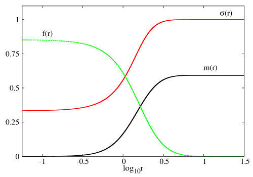
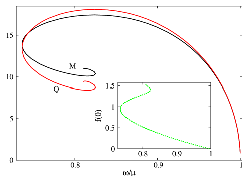
Figure 1: Spherically symmetric gravitating $\mathrm{O}(3)$ solitons. (Left panel) The radial profile functions of an illustrative solution, which has $w/\mu=0.74$. (Right panel) The mass and Noether charge as function of $\omega$. For both panels, $\alpha=1/\sqrt{2}$.

As usual with boson stars, there are fundamental states, for which the scalar fields profile has no nodes and excited states, labelled by the number of such nodes. Indeed, for given $\omega,\alpha$, the solutions form a discrete set, labelled by the number of nodes, $n$, of the function $f$. Here and also in the spinning case we will always focus on fundamental modes. A typical profile is shown in Fig. 1 (left panel), for a nodeless solution.

The domain of existence of such solitons, in an ADM mass $vs.$ frequency diagram is shown in Fig. 1 (right panel), for the illustrative value $\alpha=1/\sqrt{2}$ and $n=0$. The plot also shows the Noether charge and the value of the scalar fields at the origin. This domain of existence corresponds to a spiral, a typical pattern for boson star solutions and other gravitating solitons. The solitons exist for some restricted set of values of the angular frequency $\omega\in\left[\omega_{\mathrm{min}}\simeq 0.737,\omega_{\mathrm{max}}=1\right]$. The upper critical value $\omega_{\mathrm{max}}=1$ corresponds to the particular choice of the potential of the model (2.2). This can be confirmed by introducing a complex scalar field $\Psi$ as $\Psi=\phi^{1}+i\phi^{2}$. Then the matter Lagrangian (2.2) with the rescaling done before and taking into account the sigma model constraint (2.3) becomes, to first order in $\Psi$:

$$\mathcal{L}_{\rm m}\simeq\frac{1}{2}\partial_{\mu}\Psi\partial^{\mu}\Psi^{*}+\frac{\mu^{2}}{2}|\Psi|^{2}\ ,$$ (3.10)

where the effective mass used in numerics is $\mu=1$. Since $\omega^{2}\leqslant\mu^{2}$ is a bound state condition, the maximal frequency is $\omega_{\rm max}=1$. In this limit the spinning solitons smoothly approach perturbations around Minkowski spacetime, with the ADM mass $M$ tending to zero. Indeed, linearizing the scalar field equation (2.5) one can see that the profile function decays asymptotically as $f\sim e^{-\sqrt{1-\omega^{2}}r}$, becoming delocalized as $\omega\to 1$. This is usually referred to as the Newtonian limit.

Starting from the Newtonian limit in Fig. 1 (right panel), in which limit the function $f(r)$ becomes very close to zero and the solution trivialises, at some intermediate frequency $\omega_{\rm Mmax}$, a maximal mass is attained. Similarly to the mini boson stars case, there is also a minimal frequency, $\omega_{\rm min}$, below which no solutions are found. The solutions in between the Newtonian limit and $\omega_{\mathrm{min}}$ compose the first (forward) branch. At $\omega_{\mathrm{min}}$ the curve backbends and a second (backward) branch is found. A multi-branch structure ensues, with a third (forward) branch visible in Fig. 1 (right panel), providing an overall inspiral-type pattern for the line of solutions. Likely, the spiral approaches, at the centre, a critical singular solution with $f(0)=\pi/2$. We remark that, as a rule of thumb, as one advances along the spiral one is moving towards the strong gravity region where the solitons become more compact along the forward branches and slightly less compact along the backwards branches - see, $e.g.$ the bottom panels of Fig. 1 in [62]. On the other hand, the central value of the scalar field increases monotonically along the spiral, $cf.$ inset in Fig. 1 (right panel), as in other boson star models, $cf.$ inset in bottom panels of Fig. 1 in [62].

As a final remark concerning the spherical case, following the approach in [63], one can prove these spherical solitons do not possess generalizations with an event horizon at their center: $i.e.$ there are no spherically symmetric BHs with $\mathrm{O}(3)$-sigma model hair.

3.2 Spinning solitons - domain of existence

Taking $m\geqslant 1$, we obtain spinning solitonic solutions. The dependency of these solutions on the angular frequency $\omega$ is qualitatively similar to that just described for the spherical solitons and also observed in spinning boson star models - see the outermost solid blue line in the left panel of Fig. 2. Again we focus on fundamental modes. A recent study of excited spinning boson stars and Kerr BHs with synchronised hair has been discussed in [64].

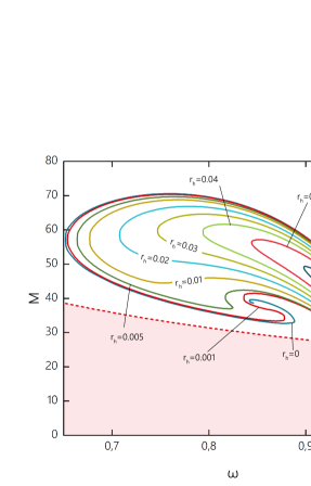
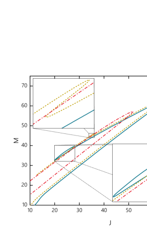
Figure 2: ADM mass $M$ $vs.$ (left panel) the angular frequency $\omega$ or (right panel) the angular momentum $J$. Here $m=1$ and $\alpha=0.5$, whereas $r_{h}$ varies. In the left panel, the shaded area corresponds to the domain of existence of vacuum Kerr BHs, the red dashed line to the extremal vacuum Kerr BHs, and the blue dashed line to the existence line: the subset of vacuum Kerr BHs that can support test field, stationary scalar clouds of the linear, massive, Klein-Gordon equation, with zero nodes and angular quantum numbers $\ell=1=m$, of the spheroidal harmonics [27].

Starting from the Newtonian limit, we observe that, as the angular frequency decreases from $\omega_{\rm max}=1$, the ADM mass of all solutions increases approaching its maximum at some value of frequency $\omega_{\rm Mmax}$. From that point onwards the mass decreases until the minimum frequency $\omega_{\mathrm{min}}$ is reached. Using the same nomenclature as before, the solutions in between the Newtonian limit and $\omega_{\mathrm{min}}$ compose the first (forward) branch. At $\omega_{\mathrm{min}}$ the curve backbends into a second (backward) branch. A third (forward) branch and a fourth (backward) branch are visible in Fig. 2, making up a spiral towards a limiting solution at the center of the spiral (challenging to obtain numerically). This mimics closely what has been found for both rotating and non-rotating boson stars (see $e.g.$ [28]) as well as for other gravitating solitons ($e.g.$ Proca stars [65]); the location and the shape of the spiral depend on the gravitational coupling strength $\alpha$ [55, 21, 22].

The blue solid curve in the right panel of Fig. 2 shows the ADM mass of the spinning solitons as a function of their total angular momentum. Again, the pattern follows closely that observed for spinning boson stars - see $e.g.$ [28]. Along the first branch both mass and angular momentum increase until the maximal ADM mass is attained; then the trend inverts and both mass and angular momentum decrease until the minimum ADM mass attained along the second (backward) branch. Another inversion follows and so on, revealing a zig-zag type structure.

In summary, the solitonic solutions of the $\mathrm{O}(3)$ sigma model mimic closely those of the more familiar mini boson stars. Boson stars with a $Q$-ball type potential also have similar features, but admit a non-trivial flat space limit, where they become $Q$-ball solutions. The spinning solitons of the non-linear $\mathrm{O}(3)$ sigma model trivialise in the flat spacetime limit, as mini-boson stars do.

3.3 Hairy black holes - domain of existence

Let us now turn to the hairy black hole solutions we constructed numerically. The problem has four input parameters, three of them continuous ($\alpha,r_{h},\omega$) and one discrete $m$. We have obtained more than 4000 solutions in order to study how the solitons and the hairy BHs depend on each of these parameters. To simplify our analysis, we mainly consider the spinning hairy BHs with winding number $m=1$, but below we shall also exhibit some solutions with $m\geqslant 1$.

The left panel of Fig. 2 exhibits the variation of the ADM mass of the spinning hairy BHs, at a fixed value of the gravitational coupling $\alpha=0.5$, versus the angular frequency $\omega$, along some lines of constant $r_{h}\neq 0$. First observe that the hairy BHs smoothly connect with the spinning solitons. Concerning the structure of the $r_{h}=$ constant lines, part of the description provided above for the solitonic limit still applies: we again observe that, as the angular frequency decreases from $\omega_{\rm max}$, the mass of all solutions increases approaching its maximum at some value of frequency $\omega_{\rm Mmax}$. This maximal mass decreases as $r_{h}$ increases. The behaviour of the $r_{h}=$constant curves beyond $\omega_{\rm Mmax}$ depends on the value of $r_{h}$.

For very small values of $r_{h}$ the spiral type critical behavior observed in the solitonic limit changes. There is still a multibranch structure; but instead of terminating at some central limiting solution, the plot shows that after three backbendings a fourth branch terminates at an upper critical value of the angular frequency $\omega_{\rm end}<1$, see Fig. 2 (left panel). In this limit, the scalar field trivializes and we recover a Kerr BH solution with the corresponding value of $r_{h}$ and that can support $\mathrm{O}(3)$ non-trivial configurations as test field solutions. This subset of Kerr BHs (as one varies $r_{h}$) defines the existence line, which, since the field becomes small, by virtue of (3.10) coincides with that found in the Einstein-(complex, massive)-Klein-Gordon theory. We call this the Kerr limit. This behaviour is qualitatively similar to that observed for other models of Kerr BHs with synchronised [27, 28].

As $r_{h}$ increases, the multibranch structure gives place to a two-branch scenario, with the first (upper, forward) branch connected to the perturbative excitations at $\omega_{\rm max}=1$ and the second (lower, backward) branch ending on the Kerr solution as $\omega\to\omega_{\rm end}$. The minimum value of the angular frequency $\omega_{\rm min}$ is increasing as $r_{h}$ increases; at some point the frequency $\omega_{\rm Mmax}$ which corresponds to the maximal value of the ADM mass along the constant $r_{h}$ line, becomes the minimal allowed frequency $\omega_{\rm min}$. Also, the maximum value of the frequency along the second branch $\omega_{\rm end}$ is slowly increasing and it approaches $\omega_{\rm max}=1$ as the loop shrinks to zero. Fig. 2 (left panel) presents the domain of existence we have just described. A very similar behaviour was recently described for excited Kerr BHs with synchronised scalar hair [64]. In the right panel of Fig. 2 we see the aforementioned zig-zag type structure remains for sequences of hairy BHs with $r_{h}={\rm constant}\neq 0$.

3.4 Some physical properties of the solutions

Having analysed the domain of existence of the solitons and hairy BHs found in the $\mathrm{O}(3)$ sigma model, which in particular shows their global quantities $M,J$, let us now consider some other basic physical properties of the solutions.

In Fig. 3 (left panel) we plot the scalar field profile function for two illustrative hairy BHs, both with the same value of $r_{h}$ but one on the first (forward) branch and another on the second (backward) branch. The figure illustrates two features. Firstly, that the scalar field distribution is the typical toroidal pattern of spinning boson stars, with a clear maximum along the equator at some radial distance and a suppression of the profile function for larger latitudes (the field vanishes along the symmetry axis). Secondly, that going along the spiral (away from the Newtonian limit), the solutions become more compact and the scalar field attains larger values.

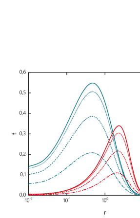
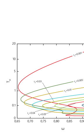
Figure 3: (Left panel) Scalar field profile function $f(r,\theta)$ of two hairy BH solutions with $r_{h}=0.01,~{}w=0.8$, one on the first forward branch (red curves) and another on the second backward branch (blue curves) branches, for several values of $\theta=\textrm{const}$. (Right panel) Hawking temperature $T_{H}$ of hairy BHs, as function of the angular frequency for a set of values of the horizon radius $r_{h}$. All solutions have $\alpha=0.5$, $m=1$.

In the right panel of Fig. 3 we exhibit the Hawking temperature for the same solutions that were plotted in the domain of existence, $cf.$ Fig. 2. One observes that, in the Kerr limit the solutions with the smallest $r_{h}$ have the smallest temperature. This is consistent with the distribution of the endpoint of the curves along the existence line, observed in the left panel of Fig. 2, where the smallest $r_{h}$ is the one closest to the extremal Kerr solutions ($cf.$ the $q=0$ line in Fig. 2 in [27]). In the Newtonian limit, on the other hand, BHs become Schwarzschild like and $r_{h}$ is a good measure of their size. Then the largest BHs have the lowest temperature, as expected.

The toroidal structure of the matter distribution exhibited in the left panel of Fig. 3 has another interesting manifestation. Similarly to what has been observed for spinning boson stars and Kerr BHs with synchronised hair [43] toroidal ergo-regions appear in the spinning solitons and hairy BHs of the $\mathrm{O}(3)$ model. These toroidal ergo-regions are delimited by an ergo-surface, defined as the zero locus of the time-like Killing vector $\xi\cdot\xi=0$, or

$$g_{tt}=-F_{0}+\sin^{2}\theta F_{2}W^{2}=0\,.$$ (3.11)

The analysis of the ergo-regions of the spinning boson in [43] showed that these solitons do not have an ergo-region in the vicinity of the Newtonian limit. Moving towards the strong gravity region, however, they develop an ergo-region still in the first forward branch, after the maximum ADM mass. The topology of the corresponding ergo-region is always an ergo-torus, $S^{1}\times S^{1}$. The hairy BHs – that connect continuously to the spinning boson stars in this model – can either have a Kerr-like ergo-region, delimited by a (topological) 2-sphere, $S^{2}$, or an ergo-Saturn, with topology $S^{2}\bigoplus(S^{1}\times S^{1})$. The former (latter) hairy BHs can be thought as a superposition of a rotating horizon with a spinning boson star without (with) a toroidal ergo-region.

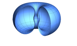
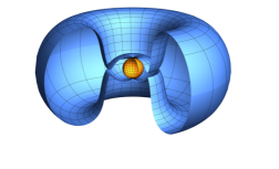
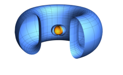
Figure 4: Illustration of the ergo-surfaces of some selected solutions. (Upper left panel) Spinning soliton along the second (backward) branch with $\omega=0.8$; (upper right panel) hairy BH along the first (forward) branch with $r_{h}=0.01$ and $\omega=0.8$; (lower left panel) hairy BH along second (backward) branch with $r_{h}=0.01$ and $\omega=0.7$; (bottom right panel) hairy BH along the second (backward) branch with $r_{h}=0.01$ and $\omega=0.685$. In the last three plots the event horizon is plotted as a yellow surface.

Using our numerical data we have found the solutions of equation (3.11) unveiling a qualitatively similar picture to that in [43]. Firstly, we observe that on the forward branch, the axially-symmetric rotating boson stars with $r_{h}=0$ appear to possess no ergosurfaces. However, on the backward branch they develop an $S^{1}\times S^{1}$ ergo-surface (ergo-torus) - Fig. 4, left upper panel. This is a pattern also observed in other boson star models, with a $Q$-ball type potential [21, 22].

On the other hand, spinning hairy BH solutions of the $\mathrm{O}(3)$ model, both on the first forward branch and on most of the secondary branches possess a Kerr-like ergo-surface with $S^{2}$ topology - Fig. 4, right upper panel. At some point along the spiral, however, the spinning hairy BHs develop an ergo-torus in addition to the $S^{2}$ ergo-sphere, thus giving rise to an ergo-Saturn, just as in [43] - Fig. 4, bottom panels. A similar pattern is observed for the hairy BH solutions of the Skyrme model recently analysed in [54].

Moving on with our analysis, we now consider the variation of the solutions with the coupling $\alpha$. In Fig. 5 we exhibit the scaled mass $M\alpha^{2}$ of the hairy BH solutions at a fixed value of the angular frequency $\omega$ versus the gravitational coupling constant $\alpha$.

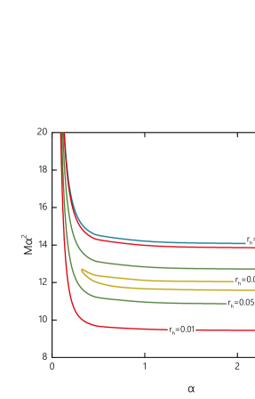
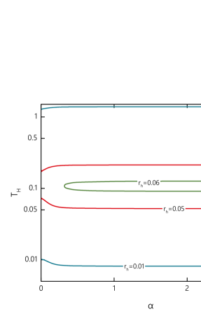
Figure 5: Scaled ADM mass $M\alpha^{2}$ (left panel) and Hawking temperature $T_{H}$ (right panel) $vs.$ the gravitational coupling constant $\alpha$, for a set of values of the horizon radius $r_{h}$, for hairy BHs of the $\mathrm{O}(3)$ model with $m=1$ and $\omega=0.9$.

Firstly, we do not find evidence for a maximal critical value of $\alpha$; $i.e.$, the solutions appear to exist for arbitrary large values of the coupling. Secondly, both the scaled mass and the Hawking temperature of the configurations remain almost constant as $\alpha$ increases above a certain critical value. In other words, in the limit of strong gravitational coupling, the ADM mass of the solutions decreases as $M\sim\alpha^{-2}$. The scale invariance of the model is effectively restored and the profile functions of the solutions become completely independent on the strength of the gravitational interactions. Notably, this pattern is also observed in the limit $\alpha\to\infty$ both for the topologically trivial pion clouds in the Einstein-Skyrme model [51], and for rotating boson stars [21].

For solitonic solutions there are, generally, two $\alpha$-branches of solutions, which bifurcate at some value of the gravitational coupling. However, as the angular velocity becomes relatively high, $\omega\sim 0.95$, we observe just a single branch of solitonic solutions. This branch terminates at some small finite value of the coupling $\alpha$, wherein the mass and the angular momentum diverge like $\alpha^{3}$. Indeed, in the $\mathrm{O}(3)$ non-linear sigma model the spinning solitons do not possess a non-trivial flat space limit.

For the hairy BHs we can also find two $\alpha$-branches of solutions, which, for small values of $r_{h}$, are disconnected - Fig. 5. As $r_{h}$ increases, the branches merge at some minimal value $\alpha_{\mathrm{min}}>0$; these solutions exist only as $\alpha>\alpha_{\mathrm{min}}$. The value of $\alpha_{\mathrm{min}}$ rapidly increases as $r_{h}$ increases.

Up to now we have always been discussing solutions with $m=1$. Let us briefly mention now solutions with higher windings $m>1$ - Fig. 6.

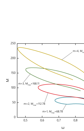
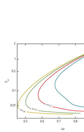
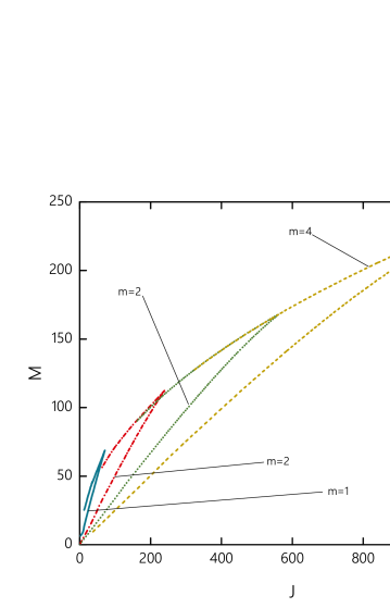
Figure 6: ADM mass $M$ (upper left panel) and Hawking temperature $T_{H}$ (upper right panel) as functions of the angular frequency $\omega$. Scaled ADM mass $vs.$ total angular momentum $J$ (bottom panel) for a set of values of the winding number $m$ for rotating hairy BHs with $r_{h}=0.01,\alpha=0.5$.

We have observed their behavior, generically, mimics the same qualitative pattern of the $m=1$ configurations. As basic trends, as the winding $m$ increases, both the ADM mass and the angular momentum increase, while the minimal allowed value of the angular frequency $\omega_{\mathrm{min}}$ decreases. Fig. 6 presents the variation of the ADM mass and Hawking temperature with $\omega$ and the mass-angular momentum relation for some selected hairy BH solutions with fixed $r_{h}=0.01$ and $m=1,2,3,4$.

Finally, let us briefly comment on the geometry of the horizon of the hairy BHs. In Fig. 4, the spatial sections of the even horizon are represented as a round $S^{2}$. Geometrically, however, these surfaces are squashed 2-spheres, rather round ones. To quantify this deformation, we have evaluated the ratio of equatorial to polar circumferences, $\epsilon=L_{e}/L_{p}$, which is exhibited in Fig. 7. Along the first forward branch the value of $\epsilon$ is slightly smaller than 1, weakly decreasing as $\omega$ decreases. Hence, as mentioned above the BHs are Schwarzschild-like in the vicinity of the Newtonian limit. The deformation becomes considerably stronger along the secondary branches, towards the Kerr limit.

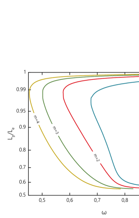
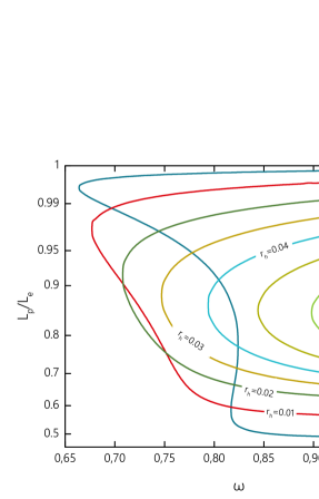
Figure 7: The ratio of the horizon circumferences $L_{e}/L_{p}$ is shown as a function of: winding number $m$ (left panel), for fixed $r_{h}=0.01$; angular frequency $\omega$ (right panel) for the forward branch solutions with $m=1$. Here all solutions have $\alpha=0.5$.

4 Conclusions

In this paper we have shown that the $\mathrm{O}(3)$ non-linear sigma-model, a simple and geometrically motivated field theory that does not admit solitonic solutions in flat spacetime, in the absence of higher order kinetic terms, can admit solitonic and hairy BH solutions when minimally coupled to gravity and when in the presence of symmetry non-inheritance. A close resemblance with the case of the massive, complex Klein-Gordon field theory has been observed. In the latter, no soliton like solutions exist in flat spacetime and, again, coupling to gravity can yield self-gravitating (both static and spinning) solitonic solutions - boson stars - and spinning hairy BHs. In fact, a parallelism on the structure of the domain of existence of solutions and physical properties between the $\mathrm{O}(3)$ sigma model and the Einstein-Klein-Gordon model has been clearly exhibited.

It is well known that field theories, in order to possess solitonic type solutions, need non-linearities. This is a necessary but not sufficient condition as shown by the absence of non-trivial solutions in the pure $\mathrm{O}(3)$ non-linear sigma-model. The soliton enabling non-linearities can have different origins: i) self-interactions of the field, as illustrated by $Q$-balls in flat spacetime; ii) higher order kinetic terms, as illustrated by the Skyrme model; iii) coupling to Einstein’s gravity, as illustrated for mini-boson stars in the massive-complex-Klein-Gordon model. For the $\mathrm{O}(3)$ non-linear sigma model case, it is well known that in the presence of higher order kinetic terms it gives rise to the topologically non-trivial Hopfions [4, 5, 66, 67, 68, 69] (point ii); here we have shown that the coupling to gravity gives rise to new regular, topologically trivial spherically symmetric and spinning solitons (point iii), and, via the synchronisation mechanism, to BHs with synchronised hair. As pointed out above, using a harmonic time dependence in field space and a sufficiently accommodating potential, it should also contain solitonic solutions in flat spacetime (point i). It would be interesting to study such solutions. One observes that, as a general pattern, symmetry non-inheritance accompanies the existence of non-topological solitons.

From the viewpoint of the hairy BH solutions found in this work, it again shows the universality of the synchronisation mechanism to yield hairy BHs in a large variety of field theory models (see another example in [70]), in different dimensions and asymptotics - see $e.g.$ [71, 72]. Thus, this mechanism can be extended to non-linear sigma models when coupled to gravity.

Finally, we remark that the $\mathrm{O}(3)$ configurations reported in this work are topologically trivial, being constructed for the simplest scalar fields ansatz (2.13). However, more general solutions, which carry a nonzero Hopf charge density, should also exist within the same model (2.1), by considering an extended $\mathrm{O}(3)$ ansatz with two essential functions. Further, a similarity of the model with Einstein-Skyrme theory [21] suggests that the pattern of the spinning self-gravitating solutions may be very involved, in particular we can expect the topologically trivial clouds may be bounded by isospinning Hopfion forming additional branches of solutions. We hope to address these problems in our future work.

References

- [1] M. Gell-Mann and M. Levy, Nuovo Cim. 16 (1960) 705.
- [2] G. H. Derrick, J. Math. Phys. 5 (1964) 1252.
- [3] T. H. R. Skyrme, Proc. Roy. Soc. Lond. A 260 (1961) 127.
- [4] L.D. Faddeev, Quantization of solitons, 1975. Princeton preprint IAS-75-QS70; also Einstein and several contemporary tendencies in the theory of elementary particles in Relativity, quanta, and cosmology, Vol.1, M. Pantaleo and F. De Finis, eds., pp. 247-266 (1979), reprinted in L. Faddeev, 40 years in mathematical physics, pp. 441-461 (World Scientific, 1995).
- [5] L. D. Faddeev, Lett. Math. Phys. 1 (1976) 289.
- [6] L. H. Kauffman, Knots and physics, River Ridge, New York, 2000.
- [7] P.M. Sutcliffe, Nature materials 16 (2017) 392.
- [8] P.M. Sutcliffe, in Ludwig Faddeev memorial volume : a life in mathematical physics. World Scientific (2018), pp. 539-547.
- [9] P.J. Ackerman and I.I. Smalyukh, Physical Review X 7 (2017) 011006.
- [10] Knots and Application, ed L. H. Kauffman, World Scientific, Singapore 1995.
- [11] D.W. Sumners, Notices A.M.S. 42, 528 (1995).
- [12] D. Harland, J. Jäykkä, Y. Shnir and M. Speight, J. Phys. A 46 (2013) 225402 [arXiv:1301.2923 [hep-th]].
- [13] R. A. Battye and M. Haberichter, Phys. Rev. D 87 (2013) no.10, 105003 [arXiv:1301.6803 [hep-th]].
- [14] R. Friedberg, T. D. Lee and A. Sirlin, Phys. Rev. D 13 (1976) 2739
- [15] S. R. Coleman, Nucl. Phys. B 262 (1985) 263 Erratum: [Nucl. Phys. B 269 (1986) 744].
- [16] I. Smolić, Class. Quant. Grav. 32 (2015) no.14, 145010
- [17] D. J. Kaup, Phys. Rev. 172 (1968) 1331.
- [18] R. Ruffini and S. Bonazzola, Phys. Rev. 187 (1969) 1767.
- [19] F. E. Schunck and E. W. Mielke, Class. Quant. Grav. 20 (2003) R301 [
- [20] M. Colpi, S. L. Shapiro and I. Wasserman, Phys. Rev. Lett. 57 (1986) 2485.
- [21] B. Kleihaus, J. Kunz and M. List, Phys. Rev. D 72 (2005) 064002
- [22] B. Kleihaus, J. Kunz, M. List and I. Schaffer, Phys. Rev. D 77 (2008) 064025
- [23] S. Yoshida and Y. Eriguchi, Phys. Rev. D 56, 762 (1997).
- [24] F. E. Schunck and E. W. Mielke, Phys. Lett. A 249 (1998) 389.
- [25] P. Grandclement, C. SomŽ and E. Gourgoulhon, Phys. Rev. D 90 (2014) no.2, 024068
- [26] C. A. R. Herdeiro, E. Radu and H. F. Runarsson, Int. J. Mod. Phys. D 25 (2016) no.09, 1641014
- [27] C. A. R. Herdeiro and E. Radu, Phys. Rev. Lett. 112 (2014) 221101
- [28] C. Herdeiro and E. Radu, Class. Quant. Grav. 32 (2015) no.14, 144001
- [29] R. P. Kerr, Phys. Rev. Lett. 11 (1963) 237.
- [30] S. Hod, Phys. Rev. D 86 (2012) 104026 Erratum: [Phys. Rev. D 86 (2012) 129902]
- [31] S. Hod, Eur. Phys. J. C 73 (2013) no.4, 2378
- [32] S. Hod, Phys. Rev. D 90 (2014) no.2, 024051
- [33] C. L. Benone, L. C. B. Crispino, C. Herdeiro and E. Radu, Phys. Rev. D 90 (2014) no.10, 104024
- [34] S. Hod, JHEP 1701 (2017) 030
- [35] R. Ruffini and J. A. Wheeler, Phys. Today 24 (1971) no.1, 30
- [36] W. E. East and F. Pretorius, Phys. Rev. Lett. 119 (2017) no.4, 041101
- [37] C. A. R. Herdeiro and E. Radu, Phys. Rev. Lett. 119 (2017) no.26, 261101
- [38] J. C. Degollado, C. A. R. Herdeiro and E. Radu, Phys. Lett. B 781 (2018) 651
- [39] P. V. P. Cunha, C. A. R. Herdeiro, E. Radu and H. F. Runarsson, Phys. Rev. Lett. 115 (2015) no.21, 211102
- [40] F. H. Vincent, E. Gourgoulhon, C. Herdeiro and E. Radu, Phys. Rev. D 94 (2016) no.8, 084045
- [41] Y. Ni, M. Zhou, A. Cardenas-Avendano, C. Bambi, C. A. R. Herdeiro and E. Radu, JCAP 1607 (2016) no.07, 049
- [42] N. Franchini, P. Pani, A. Maselli, L. Gualtieri, C. A. R. Herdeiro, E. Radu and V. Ferrari, Phys. Rev. D 95 (2017) no.12, 124025
- [43] C. Herdeiro and E. Radu, Phys. Rev. D 89 (2014) no.12, 124018
- [44] Y. Brihaye, C. Herdeiro and E. Radu, Phys. Lett. B 760 (2016) 279
- [45] J. D. Bekenstein, Phys. Rev. Lett. 28 (1972) 452.
- [46] C. A. R. Herdeiro and E. Radu, Int. J. Mod. Phys. D 24 (2015) no.09, 1542014
- [47] R. S. Ward, J. Math. Phys. 44 (2003) 3555
- [48] M. Haberichter, Classically spinning and isospinning non-linear -model solitons, PhD Thesis, University of Manchester, 2014 (unpublished).
- [49] R. A. Battye, S. Krusch and P. M. Sutcliffe, Phys. Lett. B 626 (2005) 120
- [50] R. A. Battye, M. Haberichter and S. Krusch, Phys. Rev. D 90 (2014) no.12, 125035
- [51] T. Ioannidou, B. Kleihaus and J. Kunz, Phys. Lett. B 643 (2006) 213
- [52] Y. M. Shnir, J. Exp. Theor. Phys. 121, no. 6, 991 (2015).
- [53] I. Perapechka and Y. Shnir, Phys. Rev. D 96 (2017) no.12, 125006
- [54] C. Herdeiro, I. Perapechka, E. Radu and Y. Shnir, JHEP 1810 (2018) 119
- [55] R. Friedberg, T. D. Lee and Y. Pang, Phys. Rev. D 35 (1987) 3640
- [56] Y. Verbin, Phys. Rev. D 76 (2007) 085018
- [57] C. Herdeiro, E. Radu and H. Runarsson, Phys. Lett. B 739 (2014) 302
- [58] C. A. R. Herdeiro and E. Radu, Int. J. Mod. Phys. D 23 (2014) no.12, 1442014
- [59] C.J. Lin, R.C. Weng and S.S. Keerthi, Journal of Machine Learning Research 9 (2008) 627
-
[60]
N.I.M. Gould, J.A. Scott and Y. Hu,
ACM Transactions on Mathematical Software 33 (2007) 10;
O. Schenk and K. Gärtner Future Generation Computer Systems 20 (3) (2004) 475 -
[61]
W. Schönauer and R. Weiß,
J. Comput. Appl. Math. 27, 279 (1989) 279;
M. Schauder, R. Weiß and W. Schönauer, Universität Karlsruhe, Interner Bericht Nr. 46/92 (1992). - [62] P. V. P. Cunha, J. A. Font, C. Herdeiro, E. Radu, N. Sanchis-Gual and M. Zilh‹o, Phys. Rev. D 96 (2017) no.10, 104040
- [63] I. Pena and D. Sudarsky, Class. Quant. Grav. 14 (1997) 3131.
- [64] Y. Q. Wang, Y. X. Liu and S. W. Wei, arXiv:1811.08795 [gr-qc].
- [65] R. Brito, V. Cardoso, C. A. R. Herdeiro and E. Radu, Phys. Lett. B 752 (2016) 291
- [66] J. Gladikowski and M. Hellmund, Phys. Rev. D 56 (1997) 5194
- [67] N. S. Manton and P. Sutcliffe, ’Topological solitons’, Cambridge University Press, 2004.
- [68] E. Radu and M. S. Volkov, Phys. Rept. 468 (2008) 101
- [69] Y. M. Shnir, ’Topological and Non-Topological Solitons in Scalar Field Theories’, Cambridge University Press, 2018.
- [70] C. Herdeiro, E. Radu and H. Runarsson, Class. Quant. Grav. 33 (2016) no.15, 154001
- [71] O. J. C. Dias, G. T. Horowitz and J. E. Santos, JHEP 1107 (2011) 115
- [72] Y. Brihaye, C. Herdeiro and E. Radu, Phys. Lett. B 739 (2014) 1