Reconstructing probabilistic trees
of cellular differentiation
from single-cell RNA-seq data

Abstract

Until recently, transcriptomics was limited to bulk RNA sequencing, obscuring the underlying expression patterns of individual cells in favor of a global average. Thanks to technological advances, we can now profile gene expression across thousands or millions of individual cells in parallel. This new type of data has led to the intriguing discovery that individual cell profiles can reflect the imprint of time or dynamic processes. However, synthesizing this information to reconstruct dynamic biological phenomena from data that are noisy, heterogenous, and sparse—and from processes that may unfold asynchronously—poses a complex computational and statistical challenge. Here, we develop a full generative model for probabilistically reconstructing trees of cellular differentiation from single-cell RNA-seq data. Specifically, we extend the framework of the classical Dirichlet diffusion tree to simultaneously infer branch topology and latent cell states along continuous trajectories over the full tree. In tandem, we construct a novel Markov chain Monte Carlo sampler that interleaves Metropolis-Hastings and message passing to leverage model structure for efficient inference. Finally, we demonstrate that these techniques can recover latent trajectories from simulated single-cell transcriptomes. While this work is motivated by cellular differentiation, we derive a tractable model that provides flexible densities for any data (coupled with an appropriate noise model) that arise from continuous evolution along a latent nonparametric tree.

1 Introduction

Many fundamental questions in biology invoke the question of how to describe and measure cell “state”—that is, the differences in identity between two cells with the same genome. One particularly informative measure is gene expression, i.e. the amount of RNA transcripts per gene. Recent techniques offer unprecedented biological insight by enabling massively-parallel quantification of RNA molecules at single-cell resolution (single-cell RNA sequencing, or scRNA-seq) [1, 2, 3]. However, the resulting data are noisy and zero-inflated, confounding traditional analyses [4, 5]. In this work, we employ a Bayesian approach to directly model sources of uncertainty in single-cell transcriptomic data and infer interpretable, probabilistic insight into cell state.

The particular biological phenomenon we study is cellular differentiation, the process by which a less specialized progenitor (e.g., a stem cell) gradually gives rise to cells with more specialized function. More concretely, the initial cell division is generally asymmetric, leaving one daughter cell with its stemness intact while the other cell goes on to seed a lineage of increasingly committed cells. This dynamic process can be represented as a tree, whose branches designate the incremental progression of more potent cells into various mature cell types [6]. While the lineage of a single cell can be traced back through a path of binary cell divisions, the tree we describe reflects the changing latent potential of a cell to give rise to more differentiated cells and cell fates, a dynamic process that inherently dwells along a spectrum. The importance of understanding this phenomenon is underscored by its ubiquity—for example, every cell in the human body arose through differentiation and many are continually replenished through this process, on the order of days to years [6, 7, 8, 9]. Yet, fundamental questions remain. How do identical progenitors reliably give rise to a suite of diverse cell fates? How do the dynamics of gene expression change over time and across lineages? What is the molecular program by which orchestrated changes in expression lead cells down one path over another—and how deterministic is this decision?

These systems-level questions are driven and controlled by molecular mechanisms involving coordinated regulation of gene expression. The levers of this coordination are transcription factors, whose combinatorial interactions together compose higher-level transcriptional “programs” that enact changes in cellular identity and state [6, 4]. Ultimately, we seek to gain insight into this lower-dimensional subspace (of molecular circuitry) that generates observed expression profiles—that is, how interactions among a handful of transcription factors orchestrate complex patterns of expression to drive consistent trajectories of differentiation.

To this end, we seek to infer the latent tree of cellular differentiation, and the genes that drive its topology, from scRNA-seq measurements (noisy snapshots of cell state). Since this assay is destructive to cells we cannot follow a single cell along its trajectory through time, and must instead infer this dynamic process by sampling many static snapshots of individual cells [4, 5, 10]. Further complicating analysis, any given sample of cells represents a non-uniform draw of unlabeled time points from the underlying tree of differentiation, which unfolds asynchronously [10].

In this work, we begin by reviewing previous approaches to cell trajectory reconstruction and Bayesian inference on trees, including their potential limitations, in Section 2, In Section 3, we develop a novel generative model for scRNA-seq count data arising from cells undergoing a dynamic, bifurcating differentiation process. In particular, we extend the existing Dirichlet diffusion tree model [11, 12] to incorporate a continuous distribution over pseudotime from root to leaves, filling a hole in Bayesian nonparametrics for probabilistic trees where data are not confined to discrete nodes [11, 12, 13, 14, 15, 16, 17]. In Section 4, we describe our novel MCMC algorithm, which interleaves Metropolis-Hastings and message passing steps to leverage model structure (and variable augmentation) for efficient inference. Finally, in Section 5, we present initial experiments that demonstrate the ability of our techniques to recover structure from simulated single-cell transcriptomes.

2 Background

2.1 Single-cell trajectory reconstruction

Many methods exist to infer lineage relationships from single-cell expression profiles [10]. However, most retain no notion of uncertainty, do not infer differentially expressed genes in conjunction with reconstructing the tree, or require suitable normalization or dimensionality reduction beforehand [18, 19, 20, 21, 22, 23, 24, 25, 26, 27, 28]. Moreover, the latter preprocessing decisions are generally ad hoc rather than reflecting an explicit model of data collection—compounding the lack of a framework for uncertainty. Many methods also assume a fixed number of branch points (which must be specified) [20, 19, 27, 26, 28], while others assume perfect time collection information and the ability to precisely infer cell growth [29]. Finally, adding new data from the same system is generally nontrivial, and often requires recomputation from scratch [28].

In contrast, we develop a Bayesian model of differentiation that is not fragile to preprocessing choices, since we directly model gene expression counts, and yields interpretable results for differential expression across lineages. Our approach provides a generative means of evaluating and simulating from the model, as well as a principled way to account for technical factors like zero-inflation due to gene dropout. The modularity of the generative model facilitates (streaming) incorporation of heterogenous datasets (e.g. samples enriched for stem cells versus mature cells), the ability to leverage cell time information as available, and extensions to multiple modalities of observation (e.g. multi-omic data beyond scRNA-seq). Further, we leverage Bayesian nonparametrics to learn a flexible model that expands as needed with expanded sequencing data, permitting trees of unbounded width and depth with no requirement for a priori knowledge of the number of cell fates.

2.2 Bayesian inference

Bayesian inference relies on writing out a full generative model—the prior $p(\theta)$, encoding our beliefs about the uncertainty structure over parameters $\theta$, and the likelihood $p(x\mid\theta)$, which couples the observations $x$ to the model through their dependence on the latent settings of $\theta$. Then, inference uses Bayes’ rule to invert the generative model into a mechanism for sampling from its posterior $p(\theta\mid x)$ (up to a normalizing constant, the model evidence $p(x)$, which is generally intractable). The posterior represents the density over the hidden parameters of interest, given the observations we have in hand. Concretely, here we observe cell expression profiles ($x$), and aim to recover the topology, times, and latent states of all cells and their underlying tree of differentiation potential (collectively, $\theta$).

2.3 Probabilistic latent tree models

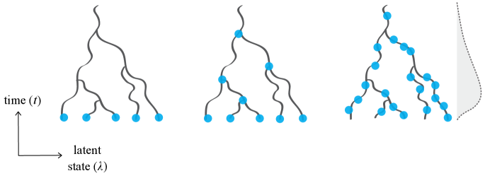
Figure S1: Categories of probabilistic latent tree-structured models. Existing Bayesian tree models (left & middle) did not fit our desiderata for observations generated continuously over a latent tree, rather than confined to discrete nodes, so we derive a novel tree-structured generative process (right). Concretely, from left to right, we depict (1) “latent ancestry” models, where data is generated only at the leaves (e.g. Dirichlet [11, 12] or Pitman–Yor [13] diffusion trees, hierarchical Dirichlet process [15], Kingman’s coalescent [14]), (2) hierarchical clustering models, where data is generated at the nodes of the tree (nested Chinese restaurant process [16], tree-structured stick breaking process [17]), and (3) our augmented Dirichlet diffusion tree model, which—in contrast—admits a continuum of latent states over the full tree according to a continuous time distribution on the unit interval (inset far right).

Previous approaches to Bayesian modeling of latent tree densities assume data are generated either only at the leaves (e.g. Dirichlet [11, 12] or Pitman–Yor [13] diffusion trees, hierarchical Dirichlet process [15], Kingman’s coalescent [14]) or only at the nodes of the tree (nested Chinese restaurant process [16], tree-structured stick breaking process [17]) (Appendix A, Figure S1, left and center). In contrast, we seek to model data arising from a more challenging regime in which observations are generated continuously over the entire tree, from root to leaves (Appendix A, Figure S1, right). Further, we seek the flexibility to model data points not as uniformly populating the tree, but rather as sporadic or dense in relation to both the “speed” at which cells undergo each transition and the relative number of cells that follow each path.

3 Bayesian generative model for cellular differentiation

Here, we describe how a cell’s observed profile in gene expression space (transcript counts $x_{\ell}$) is generated based on its latent cellular differentiation state ($\lambda_{\ell}$), where $\ell$ indexes each cell in our single-cell RNA-seq dataset. In Section 3.1, we review a previous model, the Dirichlet diffusion tree [11, 12], that provides flexible tree-structured densities. This model serves as a springboard for depicting cell trajectories in terms of latent binary branches. Then in Section 3.2, we create a new model capable of representing latent cell states as draws from continuous trajectories over a probabilistic tree. Transformations of these latent states $\lambda_{\ell}$ then directly parameterize the observation model over gene expression profiles $x_{\ell}$ from differentiating cells. Finally, in Section 3.3, we describe this model for generating noisily observed transcript counts from their “true” underlying values in each cell.

3.1 Dirichlet diffusion trees

Dirichlet diffusion trees (DDTs) provide a family of nonparametric priors over exchangeable data that arise from a latent branching process. The generative model yields tree topologies and branch times (via a hazard process) as well as latent states at and along branches (via Gaussian diffusion) [11, 12] (Appendix B). While simple in composition, the DDT has the capacity to model flexible densities; for example, its density estimation properties were previously shown to outperform both a Dirichlet process mixture model and Gaussian process density sampler [30].

Specifically, branch times and topologies are generated by iteratively simulating particles that follow a self-reinforcement scheme and deviate from existing paths according to a probabilistic divergence function, or branching rate (Appendix B). This function defines a hazard process (such that every leaf must branch by unit time) parameterized by a single scalar $\alpha$: a (positive) smoothness parameter governing whether branches are concentrated toward the root or the leaves. Following Neal [11], we assume a branching rate of $a(t)=\alpha/(1-t)$. This function defines the instantaneous chance of divergence, $a(t)\,\,\mathrm{d}t/m$, where $m$ is the number of particles that have previously traversed the given branch without diverging. Then, let

$${A}(t):=\int_{0}^{t}a(u)\,\mathrm{d}u=-\alpha\log(1-t);$$ (1)

this is the cumulative branching function. If a particle is on an existing leg of the tree bookended by times $[t_{a},t_{b}]$ and $m$ particles have previously traversed this path, the likelihood of branching by some time $t>t_{a}$ is defined by a Poisson process:

$$B_{t_{a}}(t):=\mathbb{P}(\mathrm{branch\ in}\ [t_{a},t])=1-e^{-({A}(t)-{A}(t_{a}))/m}=1-\left(\frac{1-t}{1-t_{a}}\right)^{\alpha/m}.$$ (2)

To determine if/when a new particle diverges along this branch, we calculate $t^{\prime}$ by the inverse CDF method. If $t^{\prime}$ is past the end of the branch, $t_{b}$, then the particle does not yet diverge and instead follows one of the existing child branches at time $t_{b}$ (where branch choice proportionally favors the child that previous particles have chosen). Following Knowles et al. [31], we calculate efficient likelihoods for this exchangeable distribution over topologies by reformulating the likelihood as a simple function of (cached) harmonic numbers.

Node locations (as well as the branches themselves) can then be sampled according to a Brownian motion process. Specifically, a particle that has reached $X(t)$ at time $t\in(0,1)$ will diffuse to $X(t+\,\mathrm{d}t)=X(t)+\mathcal{N}(0,\;\sigma_{0}^{2}\,\mathrm{I}\cdot\,\mathrm{d}t)$ after an infinitesimal amount of time $\,\mathrm{d}t$, for some base variance $\sigma_{0}^{2}$. Integrated over a discrete time interval $\Delta t$, $X(t+\Delta t)\sim\mathcal{N}\left(X(t),\;\sigma_{0}^{2}\,\mathrm{I}\cdot\Delta t\right)$ [11]. Thus, latent state along the tree evolves according to collective Brownian motion, where each branch event signifies the birth of two independent Brownian motion processes (conditioned on their starting location).

A draw from the distribution over ${{K}}$-leaf DDTs, marginalized over the paths between nodes, consists of a set of locations (latent states and pseudotimes) for internal and leaf nodes, indexed by $r$:

$$\tau=\{(\lambda_{r},t_{r})\}_{r=1}^{2{{K}}-1}.$$ (3)

The canonical DDT model uses these locations to model a latent hierarchy over data points, each generated from the latent state at a leaf (either marginalizing over internal nodes or instantiating them for convenience on the way to modeling the leaves) [11, 12].

3.2 Augmented Dirichlet diffusion trees for inferring cell trajectories

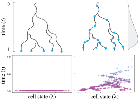
Figure 1: Classical (left) vs. augmented DDT (right). Upper: cartoon of tree and data for 1-d cell state (middle left & middle right), with ${\sf{Beta}}(5,1)$ prior over cell pseudotimes in our augmented DDT (far right). Lower: Latent cell states simulated from each model (colored by time).

We model observed expression profiles as arising from an underlying branching process. In particular, we model the hidden abstraction of cellular differentiation state, $\lambda\in\mathbb{R}^{{{G}}}$ over ${{G}}$ genes, as draws from a latent tree, and relate these smoothly evolving latent vectors to the observations through an appropriate noise model (detailed in Section 3.3). Next, we describe in more detail the generation of $\lambda_{\ell}:=[\lambda_{\ell}^{(1)},\ldots,\lambda_{\ell}^{({{G}})}]$ for genes $1,\ldots,{{G}}$ per cell, $\ell$.

As classically formulated, the DDT specifies flexible densities for data generated at the leaves of a binary tree [11] (Figure 1, left). We extend the Dirichlet diffusion tree to provide flexible densities that generate latent values (cell states) according to a continuous-time distribution over the full tree (Figure 1, right).

Recall that a draw from the DDT process yields a set of locations at discrete nodes, as well as a means of sampling all countably infinite locations between nodes (Section 3.1). In practice, we do not need the full continuum of branch locations (gray lines, Figure 1) but rather focus on that of each cell (blue dots, right, Figure 1). Therefore, our algorithm instantiates the set of tree nodes, $\mathcal{T}$, and additionally instantiates only those branch locations that correspond to cells. We can think of each location, or point, in the tree as a pair comprising the state $\lambda$ (horizontal axis in Figure 1) and pseudotime $t$ (vertical axis). Thus, cell state $\lambda_{\ell}$ can be seen as a projection of that cell’s overall location in the tree, $(\lambda_{\ell},t_{\ell})$.

In our case, the number of leaves (cell fates) is no longer fixed to the number of data points—as in a classical DDT—so we add a prior to regularize tree complexity, e.g. ${{K}}\sim 1+{\sf{Poiss}}({{K}}_{0})$, where ${{K}}$ corresponds to the number of particles that generate the DDT (i.e. the number of leaves). Additionally, we replace the canonical origin (typically set to the ${{G}}$-dimensional zero vector at time $0$ [11, 12]) with some initial root location $(\mu_{0},0)$, corresponding to a typical value for the data. Here, we leverage prior knowledge about average expression profiles for stem cells (which can be experimentally enriched and sequenced for this purpose, or readily identified among a broader dataset). To allow for gene-specific diffusion, we designate the diffusion variance $\sigma_{0}^{2}$ to be a length ${{G}}$ vector and place a conjugate inverse gamma prior over each component $\sigma_{0}^{2\ (g)}$.

Thus, we model differentiation as the process by which latent state vector $\mu_{0}$, characterizing the starting population of stem cells, morphs and bifurcates to give rise to a multiplicity of latent states. These latent states, in turn, characterize the diverse fates and functions of mature cells—noisily reflected by their warped distributions over gene expression space. We now have all of the ingredients to sample a set of tree nodes $\mathcal{T}$ (yet to be populated by cells) according to an augmented DDT with leaf prior ${{K}}_{0}$, concentration $\alpha$, and origin $\mu_{0}$ (as well as $\sigma_{0}^{2}$ prior parameters, elided for brevity)—which we denote ${\sf{DDT}}({{K}}_{0},\alpha,\mu_{0})$.

Given $\mathcal{T}\sim{\sf{DDT}}({{K}}_{0},\alpha,\mu_{0})$, each cell $\ell$ diffuses down this tree, navigating branches according to a rich-get-richer scheme, until a random time point (detailed in Appendix C). Specifically, we draw $t_{\ell}\sim F(\cdot)$, where $F$ is some distribution over $[0,1]$ encoding our belief about how cells are distributed over the tree. For example, we expect hematopoietic samples to be skewed toward mature cells [32], so might choose $F={\sf{Beta}}(4,1)$. The cell’s location in the tree at this time yields a latent cell state $\lambda_{\ell}\in\mathbb{R}^{{{G}}}$ according to the Brownian bridge defined by its Markov blanket. Namely,

$$\lambda_{\ell}\sim\mathcal{N}\left(\lambda_{a}+\frac{t_{\ell}-t_{a}}{t_{b}-t_{a}}(\lambda_{b}-\lambda_{a})\;,\;\;(t_{\ell}-t_{a})\left(1-\frac{t_{\ell}-t_{a}}{t_{b}-t_{a}}\right)\sigma_{0}^{2}\,\mathrm{I}\right),$$ (4)

for (cell or node) locations $\{(\lambda_{a},t_{a}),(\lambda_{b},t_{b})\mid t_{a}<t_{b}\}$ bookending cell $\ell$ (see Appendix B for more details about how the Brownian bridge formulation follows naturally from the properties of the DDT). Finally, we sample the cell’s observed expression profile $x_{\ell}\in\mathbb{N}^{{{G}}}$ given $\lambda_{\ell}$ according to some noise model, defined below (Section 3.3). Here, we make the simplifying assumption that genes are expressed independently conditioned on the latent structure of differentiation. Importantly, this generation scheme captures the desired behavior that we can model vastly different probabilities of observing a cell along certain intervals (not only specific time intervals, but also specific branches)—accurately reflecting the biological variance in differentiation “velocities” and in the popularity of various cell fates.

3.3 Observation model for single-cell RNA-seq

Now we need a way to connect the noisy scRNA-seq cell snapshots we observe to our tree-structured abstraction over the latent dynamics of cell state. Consider a single cell containing a set of messenger RNA (mRNA) transcripts corresponding to each gene that is currently expressed—some subset of all ${{G}}$ genes in its genome. We posit that, for a particular cell type, the discrete count $M$ of transcripts of a particular gene $g$ has a Poisson distribution with rate $\lambda^{(g)}$: $M\sim{\sf{Poiss}}(\lambda^{(g)}).$

Throughout the workflow for droplet-based sequencing [1, 2, 3], the current state of the art for single-cell transcriptomics, there are several processes known to affect accurate observation of $M$ [4, 5, 33] (Appendix D). In brief, transcripts must hybridize (with probability $p_{h}$) to a primer containing an i.i.d. uniform primer-specific barcode (unique molecular identifier, or UMI) [1], must be amplified (w.p. $p_{d}$) over the course of $R$ rounds of PCR, and must hybridize to the flow cell for sequencing (w.p. $p^{\prime}_{h}$). Since the original quantity $M$ was Poisson distributed, we can use the thinning property and the marking property of Poisson processes to show that the number attached to each unique UMI and ultimately sequenced is

$$M_{1},\dots,M_{{N_{\mathrm{UMI}}}}\overset{\textrm{{i.i.d.}}}{\sim}{\sf{Poiss}}\left(\frac{(1+p_{d})^{R}\,p^{\prime}_{h}\,p_{h}\,\lambda^{(g)}}{{N_{\mathrm{UMI}}}}\right),$$ (5)

where ${N_{\mathrm{UMI}}}$ is the theoretical number of distinct UMIs (i.e., $4^{\text{\#basepairs}}$). Finally, transcripts are quantified by aligning sequences to a reference genome, resulting in an overall count for this particular gene of $x^{(g)}=\sum_{i=1}^{{N_{\mathrm{UMI}}}}\mathds{1}\left[M_{i}>0\right].$ The distribution of this quantity has a closed-form expression:

$$x^{(g)}\sim{\sf{Binom}}\left({N_{\mathrm{UMI}}}\;,\;\;1-e^{-q\lambda^{(g)}}\right)\qquad\textrm{ with }\qquad q:=\frac{(1+p_{d})^{R}\,p^{\prime}_{h}\,p_{h}}{{N_{\mathrm{UMI}}}},$$ (6)

where $q$ is a hyperparameter accounting for gene dropout (optionally, $q^{(g)}$, with gene index $g$ also superscripting the probabilities on the right). Due to experimental dropout and natural gene regulation, the observed expression profile for cell $\ell$, $x_{\ell}:=[x_{\ell}^{(1)},\ldots,x_{\ell}^{({{G}})}]$, is a sparse vector of digital counts with $G\approx 20,000$ (for human cells) [4, 5, 33]. In practice we model a subset of the most variable genes, since genes with low variance over sampled profiles contain little information to resolve cell states along a trajectory.

Notably, latent state $\lambda_{\ell}$ drawn from a tree is in $\mathbb{R}^{{G}}$ (Section 3.2), whereas the vector of Poisson rate parameters for gene expression must be nonnegative. So, we replace the original Poisson parameter per gene with $h(\lambda^{(g)})$ for some link function $h:\mathbb{R}\to\mathbb{R}_{\geq 0}$. This maneuver enables us to model states along the tree as unconstrained reals, while preserving the necessary sign in the observation model (Equation 6). For efficient inference, we derive a link function that permits Pólya-gamma augmentation [34] for conditional conjugacy (elaborated in Section 4 and Appendix E).

Conveniently, since cell state $\lambda_{\ell}$ drawn from a diffusion tree is conditionally Gaussian, the dropout parameter $q^{(g)}$ (which acts as a per-gene linear scalar in the observation model) can be absorbed by the diffusion variance $\sigma_{0}^{2}$ and therefore learned.

4 Inference

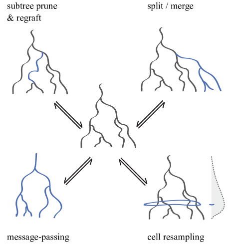
Figure S2: Cartoon overview of moves made by our inference algorithm. Upper: Moves that resample latent topology—changing internal structure (subtree prune & regraft) or the size of the tree (split/merge). Lower: Moves that resample latent locations—either cell and node latent states (message passing), or cell times and latent states (cell resampling).

Having specified the generative model, we derive a Markov chain Monte Carlo sampler to approximate the Bayesian posterior over parameters of interest (as in Section 2.2). Specifically, we aim to recover tree topology and cell locations (rates, pseudotimes, and branches)—collectively, $\theta$—given the observed cell profiles—$x$. Here, we describe our inference algorithm for efficient mixing over trees, beginning with the design of Metropolis-Hastings proposals for structure-learning and ending with a message-passing framework for exact belief propagation of latent cell and node states. In practice, we cycle through these steps uniformly at random but linger on cell resampling for enough iterations such that every cell is resampled in expectation (per cluster of cell resampling moves). See Appendix A, Figure S2 for a graphical summary of the algorithm.

Cell resampling:  In the original DDT model, each data point is always fixed to a particular leaf, and latent states are resampled during inference by rearranging the underlying tree structure. However, we face the daunting challenge of determining where each cell belongs on the tree—resampling time and branch assignment, in addition to latent state (while simultaneously learning the tree itself). To this end, this step proposes new locations for a random subset of cells, conditioned on $\mathcal{T}$. This is akin to a Gaussian mixture model over extant branches at each time slice $t_{\ell}$ and $t_{\ell}^{\prime}$. We design proposals where cells select branches with probability proportional to their likelihood, so the Metropolis-Hastings acceptance ratio reduces to the (log sum over) categorical normalizing constants at each time slice.

Motivated by empirical analysis of trace plots, we accelerate mixing by making proposals that simultaneously resample all cells within randomly sized time partitions, interleaved with occasional proposals that simultaneously resample cells on a single branch. Intuitively, this strategy is advantageous because Brownian motion of cell states at a given time is dependent on the placement of neighboring cells on each branch. Thus, we are doomed to slim acceptance of proposals unless we give an entire region of cells the opportunity to switch branches (in random order). We also increase acceptance of cell proposals by using a variable augmentation scheme to sample new cell states (see message passing, below).

While a proposal of this sort is not strictly necessary for inference on the original DDT model, a modification of this move could improve mixing by jumping between states that would otherwise be separated by many moves, potentially with unlikely intermediate transitions. Specifically, tailored for the original DDT model, this step would entail proposing “leaf swaps” (akin to cell resampling at fixed time $1$, but requiring a 1:1 mapping between leaves and data points at the end of each move).

Subtree prune and regraft (SPR):  This proposal, as formulated for DDTs [11, 12], detaches a random subtree and draws its new parent from the prior. However, unlike in Neal’s original formulation, we need a way to deal with the cells that fell along the deleted branch, while accounting for effects on the likelihood of neighboring cells. We supplement this move by resampling cells over the affected subtree, which is defined by the most recent common ancestor (MRCA) of the original and proposed parent nodes. By confining cell resampling to the MRCA subtree, we isolate changes to the likelihood to this local subtree (which would otherwise be induced through global effects on self-reinforcing cell paths).

Split/merge:  Whereas the original DDT pinned each data point to a leaf (therefore fixing the complexity), we need a way to grow and shrink tree depth according to the data. This step proposes growing or pruning subtrees, changing the dimension of the tree by one or more leaves (and resampling affected cells). “Split” chooses a random subtree to collapse, whereas “merge” chooses a random number of leaves to generate ${{K}}^{\prime}$, and draws from the DDT prior to generate a new ${{K}}^{\prime}$-leaf subtree that diverges from a random existing branch. As in SPR, we resample cells only over the relevant subtree to preserve cell likelihoods on the remainder of the tree.

Gibbs sampling:  We perform Gibbs updates to diffusion variance $\sigma_{0}^{2}$ (with a conjugate inverse gamma prior for Gaussians with fixed mean and unknown variance), as originally suggested by Neal [11, 12]. Here, the posterior over $\sigma_{0}^{2}$ (a global scalar, or vectorized over genes) is updated based on the relative locations of all cells and tree nodes.

Message passing:  We derive message passing to perform exact inference on node and cell states given their times and topology. Here, we leverage belief propagation on a binary tree with Gaussian emissions, made conditionally conjugate through Pólya-gamma (PG) augmentation [34] of binomial observations.

The PG trick has previously been used for conjugacy in binomial models like logistic regression [34], and has been adopted to facilitate computation for non-Gaussian potentials within a message-passing framework [35]. However, this work represents a novel synthesis with the more general algorithm for Gaussian belief propagation, originally posited for solving systems of linear equations through a probabilistic lens [36].

This augmentation scheme is made possible by the choice of an appropriate link function $h(\cdot)$ such that we can rewrite the original observation model,

$$x\mid\lambda\sim{\sf{Binom}}\left({N_{\mathrm{UMI}}},\;1-\exp\left[-q\cdot h(\lambda)\right]\right),$$ (7)

in the form amenable for the Pólya-gamma trick,

$$x\mid\varphi\sim{\sf{Binom}}\left(N,\;\frac{1}{1+\exp(-\varphi)}\right),$$ (8)

for some variable $\varphi$ with prior $\mathcal{N}(\mu,\Sigma)$. This setup is desirable because it allows us to elide the binomial likelihood in favor of more tractable distributions, by alternatingly sampling

$$\omega\mid\varphi\sim{\sf{PG}}(N,\varphi)\qquad\text{and}\qquad\varphi\mid x,\omega\sim\mathcal{N}(m_{\omega},V_{\omega}),$$ (9)

where

$$V_{\omega}=(\Omega+\Sigma^{-1})^{-1},\qquad m_{\omega}=V_{\omega}(\Sigma^{-1}\mu+x-N/2),$$ (10)

and $\Omega:=\operatorname{diag}(\omega)$ [34]. Importantly, the PG density admits efficient sampling [34].

To exploit this scheme, we choose link function $h$ such that the binomial probability term in Eq. (7) is equivalent to the sigmoidal probability in Eq. (8), for $\varphi=q\,\lambda$. Namely, $h(\cdot)$ must be

$$-\log\left(1-\frac{1}{1+\exp(-q\,\lambda)}\right)/q.$$ (11)

Note that the link function now depends on the dropout parameter. Since this reparameterization effectively scales a Gaussian random variable ($\lambda$) by a scalar ($q$), the dropout parameter can be absorbed by the diffusion variance $\sigma_{0}^{2}$ (and therefore learned, per gene or per tree). That is, we directly model the scaled proto-rates $q\,\lambda$ as latent variables sampled along the tree, rather than explicitly setting $q$ and modeling its effects.

Now, we endow each cell with an auxiliary PG variate $\omega_{\ell}\in\mathbb{R}^{{{G}}}$. Completing the augmentation scheme, we let $N={N_{\mathrm{UMI}}}$ and let $\mu,\Sigma$ be the prior over $\lambda_{\ell}$ given Gaussian diffusion on the tree; then, Eq. (9) is a valid algorithm for efficiently resampling latent cell states while leaving cell likelihoods intact.

Both cells and DDT nodes are now conditionally Gaussian and form a directed acyclic graph, so we can perform continuous belief propagation [36] to “share” information across the full tree and exactly resample all points (cells and nodes), recursively conditioned on their respective neighbors. This algorithm requires only two (subtree-parallelizable) sweeps over the tree—once to pass messages upward from leaves to root, and once to pass recomputed messages downward from root to leaves—prior to simultaneous resampling of all latent states (Appendix E).

This move supplants Neal’s original suggestion of resampling latent states associated with internal nodes via Gibbs updates (conditional on the locations of their immediate neighbors) [11, 12]. Gaussian belief propagation (with PG augmentation, if data generation from latent states at the leaves is nonconjugate) presents a valid alternative for DDTs.

Notably, Knowles et al. [31] derive a variational message passing framework for DDTs, to speed up calculation of (approximate) evidence and drive efficient search over tree structures, but their algorithm and intention are disjoint from ours. Later, the same authors use belief propagation to marginalize over internal nodes in the DDT [13], but this effort is also distinct and they do not consider the case of message passing with non-Gaussian observations.

4.1 Initialization

While MCMC is guaranteed to reach equilibrium at its stationary distribution, manufactured to be the true posterior, we can accelerate equilibration of our finite-time approximate inference algorithm by careful initialization. We initialize the sampler by drawing a tree from the DDT prior. Then, we initialize cell locations by sampling latent cell states conditioned on their corresponding data and auxiliary PG variates for each branch (at some time $t$, sampled from the time distribution or given by experiment). Finally, from these proposals, we iteratively assign cells to branches with probability proportional to their likelihoods. This strategy is equivalent to a cell resampling proposal over the full tree.

5 Experiments

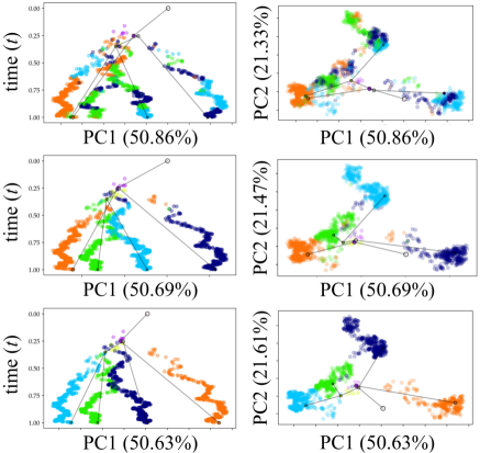
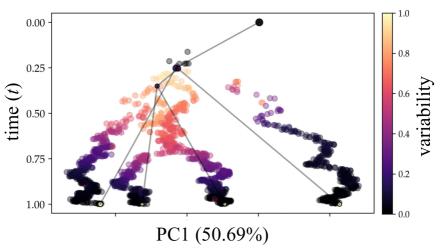
Figure 2: Shifts in $\lambda$ (left) and $x$ (right) along the first two principal components (PCs). Arrows, each corresponding to a single cell, are colored by true time and point from true to inferred value. Percentages on axis labels indicate the portion of total variation explained by that axis (i.e., that PC). Top to bottom: random, initial, MAP trees.

Figure 3: Cells colored by branch assignment. Left: PC1 of cell rate vs. time. Right: PC1 vs. PC2. Top to bottom: initial, MAP, true trees.

Figure 4: Relative branch variability per cell, based on categorical dispersion [37] across samples (normalized by choices per time slice and scaled 0-1), plotted atop the MAP tree.

In preliminary experiments, we simulated single-cell data to verify inferred parameters against known ground truth. Focusing on a restricted model (fixing tree topology and cell/node times), we demonstrate visually and quantitatively that our algorithm recovers latent trajectories. Notably, this fixed-time regime is applicable to time-course experiments where cell times are (approximately) known and tree topology is given by prior knowledge.

We simulated data for 2000 cells by sampling times $t_{\ell}\sim{\sf{Beta}}(4,1)$ and drawing latent rates $\lambda_{\ell}\in\mathbb{R}^{10}$ from an augmented DDT with 4 leaves and concentration $\alpha=3$. We then simulated expression profiles $x_{\ell}\mid\lambda_{\ell}$, as in Section 3.3 and Appendix E.

Following 9050 iterations of MCMC, we examined sampled trees (thinning=50) and assessed convergence based on trace plots. We largely recover cell parameters through our initialization procedure alone (Figure 4; procedure detailed in Section 4.1). Specifically, we highlight the discrepancy between true and inferred parameters per cell as the length of the arrow between them (visualized following PCA). We observe that cells’ deviation from ground-truth is miniscule for sampled trees in comparison to a random tree drawn with identical parameters (Figure 4, top). These arrows shrink further from initialization to the maximum a posteriori (MAP) tree (Figure 4, middle and lower, respectively), indicating that inference is approaching ground truth. We also show recovery of cell branch assignments (Figure 4), though we observe label switching. This challenge of identifiability is ubiquitous to MCMC inference of models involving clustering or other labeled components, and a sizable literature has sprung up to address it (e.g., purposeful initialization near a posterior mode) [38, 39].

To quantitatively assess tree recovery, or even summarize the posterior beyond a single mode, we need a similarity score for differentiation trees. Motivated by the desire for a means of comparing trees that may be of differing depths, such that node-matching is challenging or impossible, we propose a “triplet metric” (Appendix F). This similarity score abstracts away the underlying tree to prioritize the topology of the cells themselves and is agnostic to tree size. Further, the triplet metric is invariant to label switching. Using the triplet metric, we underscore our visual recovery of cell branches (Figure 4) by quantifying how well cell relationships agree with ground truth. Specifically, we randomly subsample triplets of cells and compare their relative locations along the inferred and true trees. Within a given triplet, we compute pairwise cell distances to determine the outlier cell on each tree (or its complement, the closest pair), where distance is given by branch length (in $t$) required to traverse the tree from one cell to the other (via their MRCA node, if not on the same branch). Then, we compute the triplet metric as the proportion of cell triplets whose outlier cell is consistent across both trees (e.g., ground-truth and sampled, or between two samples). To our knowledge, this simple method, which uses a distance metric inspired by phylogenetic trees [40], represents a new contribution to the nascent literature on comparing cell fate trajectories [28]. Here, $0$ corresponds to orthogonal cell topologies, and $1$ corresponds to perfect concurrence with ground truth. This score increased from $0.520$ to $0.828$ from the initial to MAP tree (versus $0.409$ for the random tree), indicating convergence toward true cell topology.

Finally, we can begin to reap the benefits of our probabilistic approach by examining branch uncertainty per cell across sampled trees (Figure 4), as quantified by a metric for categorical variability [37]. As expected, cells are most “confident” in their branch assignment near leaves (especially leaves that diverge earlier and are more separated in latent space), and are least certain where internal branches of the tree are close together or overlap.

6 Conclusions and future

We take a Bayesian nonparametric approach to learning cell state from inherently noisy single-cell RNA-seq data of differentiating cells. In particular, we define cell state by the latent parameterization of a distribution over gene expression space, and model these latent vectors as arising from bifurcating, self-reinforcing paths along a probabilistic tree. Motivated by the biology, this approach necessitated the development of a novel probabilistic model for data generated continuously over a tree, rather than restricted to discrete nodes or leaves. Performing efficient inference on this model also required innovations: we develop a message-passing framework for exact Gaussian belief propagation on a binary tree through Pólya Gamma augmentation and a novel MCMC sampler for learning tree structure. Simulation experiments show that our inference algorithm can resolve latent trajectories from single-cell data. Further, we demonstrate the benefits of an interpretable latent structure that includes a coherent framework for uncertainties over parameters like cell branch locations, rather than assigning each cell a single definitive label.

We are working to apply this model to data sets with noisy time-labels (e.g., experimental time points of zebrafish embryos post-fertilization), which we can use to helpfully constrain inference—as well as data sets from the more challenging regime of naturally mixed, asynchronous cells (e.g., hematopoietic, tracheal, and gut epithelial cells). We can then validate and refine the model through (experimental or natural) perturbation. By targeted experimental perturbation [41], e.g. of genes inferred as essential to a particular branch decision, we can interrogate predictions about the map from expression to tree topology. On the other hand, natural perturbations such as disease present an opportunity to compare healthy and aberrant topologies, and infer the driving discrepancies at the molecular (gene regulatory) level.

We are also developing an extension of the model that allows for a “trunk” of potential trajectories between branches (modeled as switching linear dynamical systems), such that branch points are hyperplanes (rather than zero-dimensional) and cells can approach from many distinct paths. This more complex model aims to decode cell fate decisions, by discriminating between trajectories (and their driving expression dynamics) of distinct sub-populations of cells prior to bifurcation events.

Ultimately, we are interested in the stochasticity of lineage fate specification—whether cells “commit” to (are probabilistically inclined toward) particular fates prior to branching—and in reconstructing the master regulatory programs and fitness landscapes that govern large-scale changes in cell state.

Appendix A Supplemental figures

Appendix B Dirichlet diffusion trees

The Dirichlet diffusion tree (DDT) model provides a family of priors over infinitely exchangeable data that derive from a latent binary branching process. As classically formulated, the DDT generalizes Dirichlet process mixture models for data that are hierarchical, such that data points are generated at the leaves, and internal nodes correspond to hierarchical clusters [11]. Alternately, the DDT can be constructed as the continuum limit of the nested Chinese restaurant process, or as the dual of the Kingman’s coalescent [42].

Consider a draw from the distribution over ${{K}}$-leaf DDTs. If marginalized over the paths between nodes, the sampled DDT consists of a set of discrete node locations (latent states and pseudotimes)

$$\tau=\{(\lambda_{r},t_{r})\}_{r=1}^{2{{K}}-1}.$$ (12)

Here, we use $r$ to index the locations of tree nodes (internal nodes and leaves), whereas we later use $\ell$ to index the locations of cells along the tree.

Tree topology is generated by iteratively simulating paths of particles according to a Wiener process of Gaussian diffusion (i.e. Brownian motion). Specifically, a particle that has reached $X(t)$ at time $t\in(0,1)$ will diffuse to $X(t+dt)=X(t)+\mathcal{N}(0,\;\sigma_{0}^{2}\,\mathrm{I}\cdot dt)$ after an infinitesimal amount of time $dt$, for some $\sigma_{0}^{2}$ that governs diffusion (which can be learned). Integrated over a discrete time interval $\Delta t$, then, $X(t+\Delta t)\sim\mathcal{N}\left(X(t),\;\sigma_{0}^{2}\,\mathrm{I}(\Delta t)\right)$ [11].

Following Neal [11], we assume a probabilistic branching rate of $a(t)=\alpha/(1-t)$, where $\alpha$ is a smoothness parameter related to whether branches are concentrated toward the root or the leaves. Let

$${A}(t):=\int_{0}^{t}a(u)\,\mathrm{d}u=-\alpha\log(1-t);$$ (13)

this is the cumulative branching function. If a particle is on a leg of the tree bookended by times $[t_{a},t_{b}]$, and there are $m$ particles that have traversed this path, the probability of branching at some time $t\in(t_{a},t_{b})$ is

$$B_{t_{a}}(t):=\mathbb{P}(\mathrm{branch\ in}\ [t_{a},t])=1-e^{({A}(t_{a})-{A}(t))/m}\equiv 1-\left(\frac{1-t}{1-t_{a}}\right)^{\alpha/m}.$$ (14)

To see when/if a new particle branches on an existing leg of the tree $[t_{a},t_{b}]$, we calculate $t_{r}$ by the inverse CDF method. If $t_{r}>t_{b}$, then the particle does not create a new branch on this leg and instead follows one of the existing branches at time $t_{b}$.

Overall, to create a DDT with ${{K}}$ particles:

1. Set the root of the tree to some origin $(\mu_{0},0)$, corresponding to a typical value for the data—here, we leverage prior knowledge about average expression profiles for stem cells. Draw the first particle’s leaf location as $\lambda_{\ell_{1}}\sim\mathcal{N}(\mu_{0},\;\sigma_{0}^{2}\,\mathrm{I})$.

2. For $k=2,\ldots,{{K}}$:

   1. Find the next branch point and time, $(\lambda_{b},t_{b})$, (e.g. for $k=3$, this will be where the second particle diverged) and find the number of particles $m$ that have taken this path (equivalently, the number of leaves under node $b$). Draw $u\sim{\sf{Unif}}(0,1)$ and compute a proposed branching time,

      $$t_{r}=B^{-1}_{t_{a}}(u)=1-e^{\log(1-t_{a})+\frac{m}{\alpha}\log(1-u)}.$$

   2. If $t_{r}<t_{b}$, branch at time $t_{r}$. Sample the branching location according to the Brownian bridge defined by its Markov blanket, i.e. nodes $a$ and $b$ bookending the start and end of this leg,

      $$\lambda_{r}\sim\mathcal{N}\left(\lambda_{a}+\frac{t_{r}-t_{a}}{t_{b}-t_{a}}(\lambda_{b}-\lambda_{a})\;,\;\;(t_{r}-t_{a})\left(1-\frac{t_{r}-t_{a}}{t_{b}-t_{a}}\right)\sigma_{0}^{2}\,\mathrm{I}\right).$$ (15)

      This equation derives from the properties of Brownian bridges, which describe Brownian motion tamped to prescribed values at both ends. A Brownian bridge on the interval $[0,T]$, starting at $X_{0}=0$, and ending at $X_{T}=0$ has $X_{t}\sim\mathcal{N}(0,\;t(1-t/T)\sigma_{0}^{2}\,\mathrm{I})$. We want a bridge between $\lambda_{a}$ and $\lambda_{b}$ for times $t_{r}\in(t_{a},t_{b})$, or, equivalently, $t_{r}-t_{a}\in(0,t_{b}-t_{a})$. Rewriting the time interval this way yields the variance in Eq. (15), and the mean comes from interpolating between $\lambda_{a}$ and $\lambda_{b}$ over time. Record this branch point $(\lambda_{r},t_{r})$ and sample its final leaf location from $\mathcal{N}(\lambda_{r},(1-t_{r})\,\sigma_{0}^{2}\,\mathrm{I})$. Move on to the next particle.

   3. If $t_{r}>t_{b}$, do not branch off of this leg. Instead, pick one of the two branches at time $t_{b}$ with probability equal to $m_{i}/m$, where $m_{i},\;i\in\{1,2\}$ is the number of particles that previously chose that branch. Go back to step a).

In order to model gene-specific diffusion, we let the diffusion variance $\sigma_{0}^{2}$ be a length ${{G}}$ vector and place a conjugate inverse gamma prior over each component $\sigma_{0}^{2\ (g)}$.

Appendix C Model for latent cell states conditional on a tree

A draw from the DDT process provides a set of locations at internal nodes and leaves, as well as a means of sampling all diffusive locations between nodes. In order to model cells as arising from a continuous-time distribution over a Dirichlet diffusion tree, we draw $\tau\mid{{K}}\sim{\sf{DDT}}$ and sample each cell $\ell$ as follows:

1. Draw $t_{\ell}\sim F(\cdot)$, where $F$ is some distribution over $[0,1]$ that represents our belief of how cells are distributed over the tree—e.g. for hematopoiesis we expect most cells to be near the leaves [32], so might choose something like $F={\sf{Beta}}(4,1)$.

2. Traverse the tree, starting at the root ($\lambda=\mu_{0},t=0$). At each branch point, select a branch with probability proportional to the number of cells that previously chose that branch (with counts offset by 1 for numerical stability). Stop at time $t_{\ell}$.

3. Find the points on the chosen branch (nodes or cells) that have $t_{a}<t_{\ell}<t_{b}$, with no other points in between; let $\lambda_{a}$ and $\lambda_{b}$ be the latent states of these points. For example, if this is the first cell to be added to an “empty” branch, these values are the locations of the node and parent node that define the branch. Then, sample $\lambda_{\ell}$ according to the Brownian bridge defined by its Markov blanket (points $a$ and $b$), as in Eq. (15):

   $$\lambda_{\ell}\sim\mathcal{N}\left(\lambda_{a}+\frac{t_{\ell}-t_{a}}{t_{b}-t_{a}}(\lambda_{b}-\lambda_{a})\;,\;\;(t_{\ell}-t_{a})\left(1-\frac{t_{\ell}-t_{a}}{t_{b}-t_{a}}\right)\sigma_{0}^{2}\,\mathrm{I}\right).$$ (16)

4. Finally, for each gene $g\in\{1,\ldots,{{G}}\}$, sample gene expression level

   $$x_{\ell}^{(g)}\sim{\sf{Binom}}\bigg{(}{N_{\mathrm{UMI}}}\;,\;\;1-e^{-q\,h\left(\lambda_{\ell}^{(g)}\right)}\bigg{)}$$ (17)

   as in Eq. (6), for positive link function $h$.

Completing the generative model, we also place a regularizing prior over tree complexity, i.e., number of leaves ${{K}}\sim 1+{\sf{Poiss}}({{K}}_{0})$.

Appendix D Observation model for single-cell RNA-seq

Consider a single cell containing a set of messenger RNA (mRNA) transcripts corresponding to each gene that is currently expressed. We assume that, for a particular cell type, the discrete count $M$ of transcripts of a particular gene $g$ has a Poisson distribution with rate $\lambda^{(g)}$,

$$M\sim{\sf{Poiss}}(\lambda^{(g)}).$$ (18)

For droplet-based methods, the current state-of-the-art for scRNA-seq, cells are flowed through a microfluidic device such that each cell is captured by a droplet of fluid containing a single microbead covered in a large number (roughly $10^{8}$) of barcoded DNA primers [1, 2, 3, 33]. Each primer contains a PCR handle, bead-specific barcode, and primer-specific barcode (unique molecular identifier, or UMI), as well as a poly-T tail designed to capture the 3’ poly-A tail of the processed mRNA molecules. Following cell lysis, mRNA transcripts hybridize to these randomized primers. Under the assumption that each droplet contains a single microbead and a single cell, the bead-specific barcode acts as a cell-specific barcode and the UMI (in tandem with the attached gene sequence) acts as a transcript-specific barcode [1]. As there are vastly more primers on the microbead than mRNA levels in the cell (at most roughly $10^{6}$), we assume that each transcript hybridizes with probability $p_{h}$ to a primer with an i.i.d. uniform UMI. Since the original quantity $M$ was Poisson distributed, we can use the thinning property and the marking property to show that the number attached to each unique UMI is

$$M_{1},\dots,M_{N_{\mathrm{UMI}}}\overset{\textrm{{i.i.d.}}}{\sim}{\sf{Poiss}}\left(\frac{p_{h}\lambda^{(g)}}{{N_{\mathrm{UMI}}}}\right).$$ (19)

Ideally, each $M_{i}\in\{0,1\}$; if $M_{i}>1$, we will underestimate the number of copies of mRNA for a given gene. However, this caveat is decreasingly important as ${N_{\mathrm{UMI}}}$ increases, and effectively disappears when ${N_{\mathrm{UMI}}}\gg\lambda$ (i.e. the number of unique UMIs greatly exceeds the number of mRNA transcripts for each gene). Assuming a 10 basepair UMI, this process enables digital quantification of mRNA molecules up to $4^{10}$ transcripts per gene [1].

Following reverse transcription of the bound mRNA to complementary DNA (cDNA), we use Polymerase Chain Reaction (PCR) to exponentially amplify the cDNA library [33]. Assume each molecule has some probability $p_{d}$ of successfully replicating for each round of PCR. Again using the Poisson marking/thinning property, after $R$ rounds of PCR we have

$$M^{\prime}_{1},\dots,M^{\prime}_{N_{\mathrm{UMI}}}\overset{\textrm{{i.i.d.}}}{\sim}{\sf{Poiss}}\left(\frac{(1+p_{d})^{R}\,p_{h}\,\lambda^{(g)}}{{N_{\mathrm{UMI}}}}\right).$$ (20)

The library is then loaded onto a flow cell for sequencing; we assume that each transcript hybridizes to the lawn of oligonucleotides with some probability $p^{\prime}_{h}$, yielding

$$M^{\prime\prime}_{1},\dots,M^{\prime\prime}_{{N_{\mathrm{UMI}}}}\overset{\textrm{{i.i.d.}}}{\sim}{\sf{Poiss}}\left(\frac{(1+p_{d})^{R}\,p^{\prime}_{h}\,p_{h}\,\lambda^{(g)}}{{N_{\mathrm{UMI}}}}\right).$$ (21)

Finally, following sequencing, mRNA counts per gene are quantified by aligning partial transcripts to a reference genome, with basic error correction to eliminate singletons and account for sequencing error [1, 3, 33], resulting in an overall count for this particular gene,

$$x^{(g)}=\sum_{i=1}^{{N_{\mathrm{UMI}}}}\mathds{1}\left[M^{\prime\prime}_{i}>0\right].$$ (22)

The distribution of $x^{(g)}$ has a closed-form expression:

$$x^{(g)} \sim{\sf{Binom}}\left({N_{\mathrm{UMI}}}\;,\;\;1-e^{-q\lambda^{(g)}}\right)$$ (23)

$$q :=\frac{(1+p_{d})^{R}\,p^{\prime}_{h}\,p_{h}}{{N_{\mathrm{UMI}}}},$$ (24)

where $q$ is a hyperparameter accounting for gene dropout. We can model gene-specific dropout by replacing $q$ with $q^{(g)}$ (and decorating the corresponding probabilities in Eq. (24) with gene index $g$).

Because of experimental dropout and the fact that most genes are turned off at any given time, the observed expression profile for cell $\ell$, $x_{\ell}$, is a sparse vector of digital molecular counts in roughly $\mathbb{N}^{20,000}$ (for human cells) [4, 5, 33]. In practice, we model the subset of most variable genes for a given dataset, since low variance genes provide little information to resolve cells along a trajectory.

Appendix E Pólya-gamma augmentation for latent Gaussian states with binomial emissions

We would like to leverage Pólya-Gamma augmentation to endow $p(x_{\ell}\mid\lambda_{\ell})$ binomial likelihoods with (Gaussian) conjugacy. The Pólya-Gamma (PG) trick [34] applies to the situation

$$\lambda\sim\mathcal{N}(\mu,\Sigma)\;;\;\;\;x\mid\lambda\sim{\sf{Binom}}\left(N,\frac{1}{1+\exp(-\lambda)}\right).$$ (25)

PG augmentation relies on re-writing the $1/[1+\exp(-\lambda)]$ parameterizing the binomial distribution as $\cosh$, and then recognizing that $\cosh$ is related to the moment generating function of a PG random variable [34]. If we were to choose a simple positive link function $h$ like $\exp(\cdot)$, we would end up with a $\sinh$. Instead: consider choosing a more suitable link function.

Given the setup

$$\lambda_{\ell}\sim\mathcal{N}(\mu_{\ell},\Sigma_{\ell})\;;\;\;\;x_{\ell}\mid\lambda_{\ell}\sim{\sf{Binom}}\left({N_{\mathrm{UMI}}},1-\exp\left[-q\cdot h(\lambda_{\ell})\right]\right)$$ (26)

for a single cell $\ell$’s ${{G}}$-dimensional gene expression profile $x_{\ell}$, ${{G}}$-dimensional proto-rates $\lambda_{\ell}$, and generic mean and covariance (in the case of $\lambda_{\ell}$ sampled from a DDT, these would be given by Gaussian diffusion parameters of the tree), we can define positive link function $h$ as follows:

$$h(\lambda):=-\log\left(1-\frac{1}{1+\exp(-\lambda)}\right).$$ (27)

This equation comes from setting the binomial probability we have (Eq. (26)) equal to the binomial probability form we need for PG augmentation (Eq. (25)) and solving for $h(\cdot)$. Ignoring dropout parameter $q$ momentarily, observed expression conditioned on location along the tree can now be rewritten as

$$x_{\ell}\mid\lambda_{\ell}\sim{\sf{Binom}}\left({N_{\mathrm{UMI}}},\frac{1}{1+\exp(-\lambda_{\ell})}\right).$$ (28)

Then, with the PG trick, we introduce a ${{G}}$-dimensional auxiliary variable $\omega_{\ell}$ per cell, such that we can alternatingly sample

$$\omega_{\ell}\mid\lambda_{\ell} \sim{\sf{PG}}({N_{\mathrm{UMI}}},\lambda_{\ell})$$ (29)

$$\lambda_{\ell}\mid x_{\ell},\omega_{\ell} \sim\mathcal{N}(m_{\omega,\ell},V_{\omega,\ell})$$ (30)

for covariance and mean

$$V_{\omega,\ell} =(\Omega_{\ell}+\Sigma_{\ell}^{-1})^{-1}$$ (31)

$$m_{\omega,\ell} =V_{\omega,\ell}(\Sigma_{\ell}^{-1}\mu_{\ell}+x_{\ell}-\frac{{N_{\mathrm{UMI}}}}{2})$$ (32)

where $\Omega_{\ell}:=\operatorname{diag}(\omega_{\ell})$.

Now consider the effect of dropout parameter $q$. Setting

$$1-\exp\left[-q\,h(\lambda)\right]\equiv\frac{1}{1+\exp(-q\,\lambda)}$$ (33)

(where the RHS is the desired form for PG augmentation), we obtain

$$h(\lambda)=-\log\left(1-\frac{1}{1+\exp(-q\,\lambda)}\right)/q.$$ (34)

In other words, the link function now depends on the dropout parameter (and the PG equations, Eq. (29)-Eq. (30), apply to $q\,\lambda$ rather than $\lambda$).

Note that this has the effect of scaling a normally-distributed variable ($\lambda$) by a scalar ($q$). Thus, the dropout parameter $q$ can be absorbed by the diffusion variance $\sigma_{0}^{2}$ (and therefore learned, per gene or per tree, by placing a conjugate inverse gamma prior over $\sigma_{0}^{2}$). That is, we directly model the scaled proto-rates ($q\,\lambda$) as latent values sampled along the tree, rather than explicitly setting $q$ and modeling its effects.

Appendix F Triplet metric for comparing cell distributions over trees

We need a metric to compare trees, with the challenge that trees may be of differing depths, such that node-matching is difficult or impossible. These desiderata motivate the “triplet metric,” which abstracts away the underlying tree to prioritize the topology of the cells themselves and is agnostic to tree size.

We define the triplet metric between trees $\mathcal{T},\mathcal{T}^{\prime}$ over $L$ cells as

$$\Phi(\mathcal{T},\mathcal{T}^{\prime})=\sum_{\{a,b,c\}\in\,\text{cells}}\mathbbm{1}\big{\{}\text{outlier}_{\mathcal{T}}(a,b,c)=\text{outlier}_{\mathcal{T}^{\prime}}(a,b,c)\big{\}}\bigg{/}\binom{L}{3}$$ (35)

where a triplet outlier is defined as the most distant cell of the three (i.e., the set difference between the triplet and the two cells that share the smallest pairwise path distance). Here, distance is given by the branch length (in pseudotime) required to traverse the tree from one cell to another (traveling via the most recent common ancestor node if not on same branch). This approach is loosely inspired by the use of summed branch lengths in phylogenetic literature to denote similarity between leaves (e.g., species) [40]. Thus, $\Phi$ is a metric from $0$ (no triplets agree) to $1$ (all triplets agree). In practice, we randomly subsample cell triplets for efficiency in order to approximate $\Phi$.

References

- [1] Evan Z. Macosko, Anindita Basu, Rahul Satija, James Nemesh, Karthik Shekhar, Melissa Goldman, Itay Tirosh, Allison R. Bialas, Nolan Kamitaki, Emily M. Martersteck, John J. Trombetta, David A. Weitz, Joshua R. Sanes, Alex K. Shalek, Aviv Regev and Steven A. McCarroll “Highly Parallel Genome-wide Expression Profiling of Individual Cells Using Nanoliter Droplets” In Cell 161.5, 2015, pp. 1202–1214 URL: http://dx.doi.org/10.1016/j.cell.2015.05.002
- [2] Allon M. Klein, Linas Mazutis, Ilke Akartuna, Naren Tallapragada, Adrian Veres, Victor Li, Leonid Peshkin, David A. Weitz and Marc W. Kirschner “Droplet barcoding for single-cell transcriptomics applied to embryonic stem cells” In Cell 161.5, 2015, pp. 1187–1201 DOI: 10.1016/j.cell.2015.04.044
- [3] Grace X. Y. Zheng, Jessica M. Terry, Phillip Belgrader, Paul Ryvkin, Zachary W. Bent, Ryan Wilson, Solongo B. Ziraldo, Tobias D. Wheeler, Geoff P. McDermott, Junjie Zhu, Mark T. Gregory, Joe Shuga, Luz Montesclaros, Jason G. Underwood, Donald A. Masquelier, Stefanie Y. Nishimura, Michael Schnall-Levin, Paul W. Wyatt, Christopher M. Hindson, Rajiv Bharadwaj, Alexander Wong, Kevin D. Ness, Lan W. Beppu, H. Joachim Deeg, Christopher McFarland, Keith R. Loeb, William J. Valente, Nolan G. Ericson, Emily A. Stevens, Jerald P. Radich, Tarjei S. Mikkelsen, Benjamin J. Hindson and Jason H. Bielas “Massively parallel digital transcriptional profiling of single cells” In Nature Communications 8, 2017 DOI: 10.1038/ncomms14049
- [4] Allon Wagner, Aviv Regev and Nir Yosef “Revealing the vectors of cellular identity with single-cell genomics” In Nature Biotechnology 34.11, 2016, pp. 1145–1160 DOI: 10.1038/nbt.3711
- [5] Oliver Stegle, Sarah A. Teichmann and John C. Marioni “Computational and analytical challenges in single-cell transcriptomics” In Nature Reviews Genetics 16.3, 2015, pp. 133–145 DOI: 10.1038/nrg3833
- [6] S. F. Gilbert and M. J. F. Barresi “Developmental Biology, 11th edition” Sinauer, 2016 URL: http://11e.devbio.com/
- [7] Li-Fang Chu, Ning Leng, Jue Zhang, Zhonggang Hou, Daniel Mamott, David T. Vereide, Jeea Choi, Christina Kendziorski, Ron Stewart and James A. Thomson “Single-cell RNA-seq reveals novel regulators of human embryonic stem cell differentiation to definitive endoderm” In Genome Biology 17.1, 2016 DOI: 10.1186/s13059-016-1033-x
- [8] Stuart H. Orkin and Leonard I. Zon “Hematopoiesis: An Evolving Paradigm for Stem Cell Biology” In Cell 132.4, 2008, pp. 631–644 DOI: 10.1016/j.cell.2008.01.025
- [9] Nick Barker “Adult intestinal stem cells: critical drivers of epithelial homeostasis and regeneration” In Nature Reviews Molecular Cell Biology 15.1, 2014, pp. 19–33 DOI: 10.1038/nrm3721
- [10] Robrecht Cannoodt, Wouter Saelens and Yvan Saeys “Computational methods for trajectory inference from single-cell transcriptomics” In European Journal of Immunology 46.11, 2016, pp. 2496–2506 DOI: 10.1002/eji.201646347
- [11] Radford M. Neal “Density modeling and clustering using Dirichlet diffusion trees” In Bayesian Statistics 7, 2003, pp. 619–629
- [12] Radford M. Neal “Defining priors for distributions using Dirichlet diffusion trees” In Technical Report No. 0104, Dept. of Statistics, University of Toronto, 2001
- [13] David A. Knowles and Zoubin Ghahramani “Pitman Yor Diffusion Trees for Bayesian Hierarchical Clustering” In IEEE Transactions on Pattern Analysis and Machine Intelligence 37.2, 2015, pp. 271–289
- [14] JFC Kingman “The coalescent” In Stochastic Processes and their Applications 13.3, 1982, pp. 235–248
- [15] Yee W. Teh, Michael I. Jordan, Matthew J. Beal and David M. Blei “Hierarchical Dirichlet processes” In Journal of the American Statistical Association 101.476, 2006, pp. 1566–1581
- [16] David M. Blei, Thomas L. Griffiths and Michael I. Jordan “The nested Chinese restaurant process and Bayesian nonparametric inference of topic hierarchies” In Journal of the ACM 57.2, 2010
- [17] Ryan P Adams, Zoubin Ghahramani and Michael I. Jordan “Tree-Structured Stick Breaking for Hierarchical Data” In Advances in Neural Information Processing Systems 23, 2010, pp. 19–27 URL: http://papers.nips.cc/paper/4108-tree-structured-stick-breaking-for-hierarchical-data.pdf
- [18] Laleh Haghverdi, Maren Buttner, F Alexander Wolf, Florian Buettner and Fabian J Theis “Diffusion pseudotime robustly reconstructs lineage branching” In Nature Methods 13, 2016, pp. 845–848
- [19] Manu Setty, Michelle D Tadmor, Shlomit Reich-Zeliger, Omer Angel, Tomer Meir Salame, Pooja Kathail, Kristy Choi, Sean Bendall, Nir Friedman and Dana Pe’er “Wishbone identifies bifurcating developmental trajectories from single-cell data” In Nature Biotechnology 34, 2016, pp. 637–645
- [20] Cole Trapnell, Davide Cacchiarelli, Jonna Grimsby, Prapti Pokharel, Shuqiang Li, Michael Morse, Niall J Lennon, Kenneth J Livak, Tarjei S Mikkelsen and John L Rinn “The dynamics and regulators of cell fate decisions are revealed by pseudotemporal ordering of single cells” In Nature Biotechnology 32, 2014, pp. 381–386
- [21] Xiaojie Qiu, Qi Mao, Ying Tang, Li Wang, Raghav Chawla, Hannah Pliner and Cole Trapnell “Reversed graph embedding resolves complex single-cell trajectories” In Nature Methods 14.10, 2017, pp. 979–982 DOI: 10.1101/110668
- [22] Kevin R. Moon, David Dijk, Zheng Wang, William Chen, Matthew J Hirn, Ronald R Coifman, Natalia B Ivanova, Guy Wolf and Smita Krishnaswamy “PHATE: A Dimensionality Reduction Method for Visualizing Trajectory Structures in High-Dimensional Biological Data” In bioRxiv, 2017 DOI: 10.1101/120378
- [23] Alexis Boukouvalas, James Hensman and Magnus Rattray “BGP: Branched Gaussian processes for identifying gene-specific branching dynamics in single cell data” In bioRxiv, 2017 DOI: 10.1101/166868
- [24] Joshua D. Welch, Alexander J. Hartemink and Jan F. Prins “SLICER: inferring branched, nonlinear cellular trajectories from single cell RNA-seq data” In Genome Biology 17, 2016 DOI: 10.1186/s13059-016-0975-3
- [25] Eugenio Marco, Robert L. Karp, Guoji Guo, Paul Robson, Adam H. Hart, Lorenzo Trippa and Guo-Cheng Yuan “Bifurcation analysis of single-cell gene expression data reveals epigenetic landscape” In Proceedings of the National Academy of Sciences 111.52, 2014, pp. E5643–E5650 DOI: 10.1073/pnas.1408993111
- [26] Kieran R Campbell and Christopher Yau “Probabilistic modeling of bifurcations in single-cell gene expression data using a Bayesian mixture of factor analyzers” In Wellcome Open Research 2, 2017 DOI: 10.12688/wellcomeopenres.11087.1
- [27] Tapio Lönnberg, Valentine Svensson, Kylie R. James, Daniel Fernandez-Ruiz, Ismail Sebina, Ruddy Montandon, Megan S. F. Soon, Lily G. Fogg, Arya Sheela Nair, Urijah N. Liligeto, Michael J. T. Stubbington, Lam-Ha Ly, Frederik Otzen Bagger, Max Zwiessele, Neil D. Lawrence, Fernando Souza-Fonseca-Guimaraes, Patrick T. Bunn, Christian R. Engwerda, William R. Heath, Oliver Billker, Oliver Stegle, Ashraful Haque and Sarah A. Teichmann “Single-cell RNA-seq and computational analysis using temporal mixture modeling resolves Th1/Tfh fate bifurcation in malaria” In Science Immunology 2.9, 2017 DOI: 10.1126/sciimmunol.aal2192
- [28] Wouter Saelens, Robrecht Cannoodt, Helena Todorov and Yvan Saeys “A comparison of single-cell trajectory inference methods: towards more accurate and robust tools” In bioRxiv, 2018 URL: https://doi.org/10.1101/276907
- [29] Geoffrey Schiebinger, Jian Shu, Marcin Tabaka, Brian Cleary, Vidya Subramanian, Aryeh Solomon, Siyan Liu, Stacie Lin, Peter Berube, Lia Lee, Jenny Chen, Justin Brumbaugh, Philippe Rigollet, Konrad Hochedlinger, Rudolf Jaenisch, Aviv Regev and Eric Lander “Reconstruction of developmental landscapes by optimal-transport analysis of single-cell gene expression sheds light on cellular reprogramming” In bioRxiv, 2018 URL: https://doi.org/10.1101/191056
- [30] Iain Murray, David MacKay and Ryan P Adams “The Gaussian Process Density Sampler” In Advances in Neural Information Processing Systems 21 Curran Associates, Inc., 2009, pp. 9–16 URL: http://papers.nips.cc/paper/3410-the-gaussian-process-density-sampler.pdf
- [31] David A. Knowles, Jurgen Van Gael and Zoubin Ghahramani “Message passing algorithms for Dirichlet diffusion trees” In Proceedings of the 28th International Conference on Machine Learning, 2011
- [32] Iain C. Macaulay, Valentine Svensson, Charlotte Labalette, Lauren Ferreira, Fiona Hamey, Thierry Voet, Sarah A. Teichmann and Ana Cvejic “Single-Cell RNA-Sequencing Reveals a Continuous Spectrum of Differentiation in Hematopoietic Cells” In Cell 14, 2016, pp. 966–977
- [33] Aleksandra A. Kolodziejczyk, Jong Kyoung Kim, Valentine Svensson, John C. Marioni and Sarah A. Teichmann “The Technology and Biology of Single-Cell RNA Sequencing” In Molecular Cell 58.4, 2015, pp. 610–620 DOI: 10.1016/j.molcel.2015.04.005
- [34] Nicholas G. Polson, James G. Scott and Jesse Windle “Bayesian inference for logistic models using Pólya-gamma latent variables” In Journal of the American Statistical Association 108.504, 2013, pp. 1339–1349
- [35] Scott Linderman, Matthew Johnson, Andrew Miller, Ryan Adams, David Blei and Liam Paninski “Bayesian Learning and Inference in Recurrent Switching Linear Dynamical Systems” In Proceedings of Machine Learning Research 54, 2017, pp. 914–922
- [36] Danny Bickson “Gaussian Belief Propagation: Theory and Application” In Ph.D. thesis, Hebrew University of Jerusalem, 2008 URL: http://arxiv.org/abs/0811.2518
- [37] Erindi Allaj “Two simple measures of variability for categorical data” In Journal of Applied Statistics 45.8, 2018, pp. 1497–1516
- [38] A Jasra, CC Holmes and DA Stephens “Markov Chain Monte Carlo Methods and the Label Switching Problem in Bayesian Mixture Modeling” In Statistical Science 20.1, 2005, pp. 50–67
- [39] Stan team “Bayesian statistics using Stan, version 2.18.1”, 2018 URL: http://www.stat.columbia.edu/~gelman/bda.course/_book
- [40] DA Baum and SD Smith “Tree thinking: an introduction to phylogenetic biology” W.H. Freeman, 2012
- [41] Atray Dixit, Oren Parnas, Biyu Li, Jenny Chen, Charles P. Fulco, Livnat Jerby-Arnon, Nemanja D. Marjanovic, Danielle Dionne, Tyler Burks, Raktima Raychowdhury, Britt Adamson, Thomas M. Norman, Eric S. Lander, Jonathan S. Weissman, Nir Friedman and Aviv Regev “Perturb-Seq: Dissecting Molecular Circuits with Scalable Single-Cell RNA Profiling of Pooled Genetic Screens” In Cell 167.7, 2016, pp. 1853–1866 DOI: 10.1016/j.cell.2016.11.038
- [42] David Arthur Knowles “Bayesian non-parametric models and inference for sparse and hierarchical latent structure” In Ph.D. thesis, Wolfson College, University of Cambridge, 2012 URL: https://davidaknowles.github.io/documents/daknowles_thesis.pdf