The large and small scale properties of the intergalactic gas in the Slug Ly$\alpha$ nebula revealed by MUSE He ii emission observations

Abstract

With a projected size of about 450 kpc at z$\simeq 2.3$, the Slug Ly$\alpha$ nebula is a rare laboratory to study, in emission, the properties of the intergalactic gas in the Cosmic Web. Since its discovery, the Slug has been the subject of several spectroscopic follow-ups to constrain the properties of the emitting gas. Here we report the results of a deep MUSE integral-field spectroscopic search for non-resonant, extended $\text{He\,{ii}}\lambda 1640$ and metal emission. Extended He ii radiation is detected on scales of about 100 kpc, but only in some regions associated with the bright Ly$\alpha$ emission and a continuum-detected source, implying large and abrupt variations in the line ratios across adjacent regions in projected space. The recent detection of associated H$\alpha$ emission and similar abrupt variations in the Ly$\alpha$ kinematics, strongly suggest that the He ii/Ly$\alpha$ gradient is due to large variations in the physical distances between the associated quasar and these regions. This implies that the overall length of the emitting structure could extend to physical Mpc scales and be mostly oriented along our line of sight. At the same time, the relatively low He ii/Ly$\alpha$ values suggest that the emitting gas has a broad density distribution that - if expressed in terms of a lognormal - implies dispersions as high as those expected in the interstellar medium of galaxies. These results strengthen the possibility that the density distribution of intergalactic gas at high-redshift is extremely clumpy and multiphase on scales below our current observational spatial resolution of a few physical kpc.

1 Introduction

Our standard cosmological paradigm predicts that both dark and baryonic matter in the universe should be distributed in a network of filaments that we call the Cosmic Web where galaxies form and evolve (e.g., Bond et al., 1996). During the last few years, a new observational window on the densest part of this Cosmic Web has been opened by the direct detection of hydrogen in Ly$\alpha$ emission on large intergalactic scales in proximity of bright quasars (e.g., Cantalupo et al. 2014; Martin et al. 2014; Hennawi et al. 2015; Borisova et al. 2016; see also Cantalupo 2017 for a review). These two-dimensional (or three-dimensional in the case of integral-field spectroscopy) observations with spatial resolution currently limited only by the atmospheric seeing (corresponding to a few kpc at z$\sim 3$) are now complementing several decades of absorption studies (see e.g., Rauch 1998; Meiksin 2009 for reviews) albeit still on possibly different environments. The latter are limited to either one-dimensional or very sparse two-dimensional probes of the Intergalactic Medium (IGM) with spatial resolution of a few Mpc (e.g. Lee et al., 2018).

The possibility of detecting the IGM in emission by using, e.g., fluorescent Ly$\alpha$ due to the cosmic UV background, was already suggested several decades ago (e.g. Hogan & Weymann, 1987; Gould & Weinberg, 1996). However, the faintness of the expected emission is hampering the possibility of detecting such emission with current facilities (e.g., Rauch et al. 2008; see also Cantalupo et al. 2005 and Gallego et al. 2018 for discussion). By looking around bright quasars, the expected fluorescent emission due to recombination radiation should be boosted by several orders of magnitude within the densest part of the cosmic web (e.g. Cantalupo et al., 2005; Kollmeier et al., 2010; Cantalupo et al., 2012). Deep narrow-band imaging campaigns around bright quasars (e.g. Cantalupo et al., 2012, 2014; Martin et al., 2014; Hennawi et al., 2015; Arrigoni Battaia et al., 2016) and, more recently, integral-field spectroscopic campaigns with the Multi Unit Spectroscopic Explorer (MUSE) (e.g., Borisova et al. 2016; Arrigoni Battaia et al. 2018) and the Palomar/Keck Cosmic Web Imager (P/KCWI) (e.g., Martin et al. 2014; Cai et al. 2018) are finally revealing giant Ly$\alpha$ nebulae with size exceeding 100 kpc around essentially all bright quasars (at least at $z>3$ while at $z\simeq 2$ they seem to be detected more rarely, see e.g., Arrigoni Battaia et al. 2016 and Cantalupo 2017 for discussion).

The Slug nebula at z$\simeq$2.3 was one of the first, largest and most luminous among the nebulae found in these observations (Cantalupo et al., 2014). It is characterised by very bright and filamentary Ly$\alpha$ emission extending about 450 projected kpc around the quasar UM287 (see Fig.1). As discussed in Cantalupo et al. (2014) and Cantalupo (2017), the high Ly$\alpha$ Surface Brightness (SB) of the Slug would imply either: i) very large densities of cold ($T\sim 10^{4}$ K) and ionised gas (if emission is dominated by hydrogen recombinations) or, ii) very large column densities of neutral hydrogen (if the emission is due to ”photon-pumping” or scattering of Ly$\alpha$ photons produced within the quasar broad line region).

Unfortunately, Ly$\alpha$ imaging alone does not help disentangle these two emission mechanisms. Several spectroscopic follow-ups by means of long-slit observations have tried recently to detect other non-resonant lines such as $\text{He\,{ii}}\lambda 1640$ (i.e., the first line of the Balmer series of singly ionized helium; see Arrigoni Battaia et al. 2015) and hydrogen H$\alpha$ (Leibler et al., 2018) in the Slug. At the same time, the Slug Ly$\alpha$ emission has been re-observed with integral-field spectroscopy using the Palomar Cosmic Web Imager (PCWI) by Martin et al. (2015), revealing large velocity shifts that, at the limited spatial resolution of PCWI have been interpreted as a possible signature of a rotating structure on 100 kpc scales. Given the resonant nature of the Ly$\alpha$ emission, it is not clear however how much of these shifts are due to radiative transfer effects rather than kinematics. A two-dimensional velocity map of a non-resonant line would be essential to understand the possible kinematical signatures in the nebula. However, until now only long-slit detection or upper limits on H$\alpha$ or He ii1640 are available for some parts of the nebula, as discussed below.

The non-detection of $\text{He\,{ii}}\lambda 1640$ in a low-resolution LRIS long-slit spectroscopic observation of Arrigoni Battaia et al. (2015) resulted in a He ii/Ly$\alpha$ upper limit of 0.18 ($3\sigma$) in the brightest part of the nebula, suggesting either that Ly$\alpha$ emission is produced by ”photon-pumping” (the second scenario in Cantalupo et al. 2014) or, e.g., that the ionisation parameter in some part of the nebula is relatively small (log($U)<-1.5$; see Arrigoni Battaia et al. (2015) for discussion ) . Assuming a ”single-density scenario” (or a “delta-function” density distribution as discussed in this work) where cold gas is in the form of clumps, a single distance of 160 kpc and a plausible flux from UM287 this upper limit on U would translate into a gas density of $n>3$ cm^-3. However, such non-detection does not give us a constraint on the emission mechanism and is obviously limited to the small region covered by the spectroscopic slit.

By means of long-slit IR spectroscopy with MOSFIRE of part of the Slug, Leibler et al. (2018) were able to detect H$\alpha$ with a flux similar to the expected recombination radiation scenario for Ly$\alpha$. This result clearly rules out that, at least in the region covered by the slit, ”photon-pumping” has a significant contribution to the Ly$\alpha$ emission. In this case, deep He ii1640 constraints can be used to infer gas densities with some assumptions about the quasar ionizing flux.

At the same time the relatively narrow H$\alpha$ emission (with a velocity dispersion of about 180 km/s), compared to the Ly$\alpha$ line width in similar regions (showing a velocity dispersion of about 400 km/s), does suggest the presence of radiative transfer effects. The medium-resolution Ly$\alpha$ spectrum obtained by Leibler et al. (2018) using LRIS in the same study shows however a similar velocity centroid for Ly$\alpha$ and the integrated H$\alpha$, suggesting that Ly$\alpha$ could still be used as a tracer of kinematics, at least in a average sense and on large scales. Different from the PCWI spectrum, the Ly$\alpha$ velocity shifts seem very abrupt on spatially adjacent regions, hinting to the possibility of more complex kinematics than the simple rotating structure suggested by Martin et al. (2015) or that the Slug could be composed of different systems separated in velocity (and possibly physical) space.

In this study, we use MUSE (see e.g., Bacon et al. 2015) to overcome some of the major limitations of long-slit spectroscopic observations discussed above in order to obtain full two-dimensional and kinematic constraints on the non-resonant $\text{He\,{ii}}\lambda 1640$ emission and metal lines at high spatial resolution (seeing-limited). Combined with previous studies of both Ly$\alpha$ and H$\alpha$ emission, our deep integral field observations allow us to address several open questions, including: i) what is the density distribution of the cold gas in the intergalactic medium around the Slug quasar (UM287) on scales below a few kpc?, ii) what are the large-scale properties and the kinematics of the intergalactic filament(s) associated with the Slug nebula?

Before addressing these questions, we will go through a description of our experimental design, observations, data reduction and analysis in section 2. We will then present our main results in section 3 followed by a discussion of how our results address the questions above in section 4. We will then summarise our work in section 5. Throughout the paper we use the cosmological parameters: $h=0.696$, $\Omega_{\rm{m}}=0.286$, and $\Omega_{\rm{vac}}=0.714$ as derived by Bennett et al. (2014). Angular size distances have been computed using Wright (2006) providing a scale of 8.371 kpc/” at $z=2.279$. Distances are always proper, unless stated otherwise.

2 Observations and data reduction

The field of the Slug nebula (quasar UM287; Cantalupo et al. 2014) was observed with MUSE during two visitor-mode runs in P94 as a part of the MUSE Guaranteed Time of Observations (GTO) program (proposal ID: 094.A-0396) for a total of 9 hours of exposure time on source. Data acquisition followed the standard strategy for our GTO programs on quasar fields: 36 individual exposures of 15 minutes integration time each were taken applying a small dithering and rotation of 90 degrees between them (see also Borisova et al. 2016; Marino et al. 2018). Nights were classified as clear with a median seeing of about 0.8” as obtained from the measurement of the quasar Point Spread Function (PSF). The only available configuration in P94 (and subsequent periods until P100) was the Wide Field Mode without Adaptive Optics (WFM-NAO) providing a field of view of about $1\times 1$ arcmin² sampled by 90000 spaxels with spatial sizes of $0.2\times 0.2$ arcsec² and spectral resolution elements with sizes of $1.25\mathrm{\AA}$. We chose the nominal wavelength mode resulting in a wavelength coverage extending from 4750$\mathrm{\AA}$ to 9350$\mathrm{\AA}$.

At the measured systemic redshift of the Slug quasar, UM287, i.e. $z=2.283\pm 0.001$ obtained from the detection of a narrow (FWHM$=200$ km/s) and compact CO(3-2) emission line (De Carli et al, in prep.), the wavelength coverage in the rest-frame extends from about 1447$\mathrm{\AA}$ to about 2848$\mathrm{\AA}$. This allows us to cover the expected brightest UV emission lines after Ly$\alpha$ such as the $\text{C\,{iv}}\lambda 1549$ doublet (5081.3-5089.8$\mathrm{\AA}$ in the observed frame in air), $\text{He\,{ii}}\lambda 1640$ (5384.0$\mathrm{\AA}$ in the observed frame in air), and the $\text{C\,{iii}}\lambda 1908$ doublet (6257.9-6264.6$\mathrm{\AA}$ in the observed frame in air). The MgII2796 doublet is in principle also covered by our observations although we expect this line to appear at the very red edge of our wavelength range where the instrumental sensitivity, instrumental systematics and bright sky lines significantly reduce our ability to put constraints on this line, as discussed in section 4.

Data reduction followed a combination of both standard recipes from the MUSE pipeline (version 1.6, Weilbacher et al. 2016) and custom-made routines that are part of the CubExtractor software package (that will be presented in detail in a companion paper; Cantalupo, in prep.) aiming at improving flat-fielding and sky subtraction as described in more detail below. The MUSE pipeline standard recipes (scibasic and scipost) included bias subtraction, initial flat-fielding, wavelength and flux calibration, in addition to the geometrical cube reconstruction using the appropriate geometry table obtained in our GTO run. We did not perform sky-subtraction using the pipeline as we used the sky for each exposure to improve flat-fielding as described below.

These initial steps resulted in 36 datacubes, which we registered to the same frame correcting residual offsets using the positions of sources in the white-light images obtained by collapsing the cubes in the wavelength direction. As commonly observed after the standard pipeline reduction, the white-light images showed significant flat-fielding residuals and zero-levels fluctuations up to 1% of the average sky value across different Integral Field Units (IFUs). These residuals are both wavelength and flux dependent. In a companion paper describing the CubExtractor package (Cantalupo, in prep.) we discuss the possible origin of these variations and provide more details and test cases for the procedures described below.

2.1 CubeFix: flat-fielding improvement with self-calibration

Because our goal is to detect faint and extended emission to levels that are comparable to the observed systematic variations, we developed a post-processing routine called CubeFix to improve the flat-fielding by self-calibrating the cube using the observed sky. In short, CubeFix calculates a chromatic and multiplicative correction factor that needs to be applied to each IFU and to each slice within each IFU in order to make the measured sky values consistent with each other over the whole Field of View (FoV) of MUSE.

This is accomplished by first dividing the spectral dimension in an automatically obtained set of pseudo medium-bands (on sky continuum) and pseudo narrow-bands on sky lines. This is needed both to ensure that there is enough signal to noise in each band for a proper correction and to allow the correction to be wavelength and flux dependent. In this step, particular care is taken by the software to completely include all the flux of the (possibly blended) sky lines in the narrow-bands, as line-spread-function variations (discussed below) make the shape and flux density of sky lines vary significantly across the field. Then for each of these bands an image is produced by collapsing the cube along the wavelength dimension. A mask (either provided or automatically calculated) is used to exclude continuum sources. By knowing the location of the IFU and slices in the MUSE FoV (using the information stored in the pixtable), CubeFix calculates the averaged sigma clipped values of the sky for each band, IFU and slice and correct these values in order to make them as constant as possible across the MUSE FoV. When there are not enough pixels for a slice-to-slice correction, e.g. in the presence of a masked source, an average correction is applied using the adjacent slices. The slice-by-slice correction is only applied using the medium-bands that include typically around 300 wavelength layers each. An additional correction on the IFU level only is then performed using the narrow-bands on the sky-lines. This insures that the sky signal always dominates with respect to pure line emission sources and therefore that these sources do not cause overcorrections. We have verified and tested this by injecting fake extended line emission sources with a size of $20\times 20$ arcsec² in a single layer at the expected wavelengths of He ii and C iv emission of the Slug nebula, both located far away in wavelength from skylines, with a SB of $10^{-18}$ erg s^-1 cm^-2 arcsec^-2. After sky subtraction, the flux of these sources is recovered within a few percent of the original value. We note, however, that caution must be taken when selecting the width of the skyline narrow-bands if very bright and extended emission lines are expected to be close to the skylines.

In order to reduce possible overcorrection effects due to continuum sources, we performed the CubeFix step iteratively, repeating the procedure after a first total combined cube is obtained (after sky subtraction with CubeSharp as described below). The higher SNR of this combined cube allows a better masking of sources for each individual cube, significantly improving overcorrection problems around very bright sources. We stress that, by construction, a self-calibration method such as CubeFix can only work for fields that are not crowded with sources (e.g., a globular cluster) or filled by extended continuum sources such as local galaxies. CubeFix has been successfully applied providing excellent results for both quasar and high-redshift galaxy fields (including, e.g., Borisova et al., 2016; Fumagalli et al., 2016; North et al., 2017; Fumagalli et al., 2017b; Farina et al., 2017; Ginolfi et al., 2018; Marino et al., 2018).

2.2 CubeSharp: flux conserving sky-subtraction

The Line Spread Function (LSF) is known to vary both spatially and spectrally across the MUSE FoV and wavelength range (e.g., Bacon et al. 2015). Moreover, because of the limited spectral resolution of MUSE, the LSF is typically under-sampled. Temporal variations due to, e.g. temperature changes during afternoon calibrations and night-time observations, result in large slice-by-slice fluctuations of sky line fluxes in each layer that cannot be corrected by the MUSE standard pipeline method (see e.g., Bacon et al. 2015 for an example). To deal with this complex problem, other methods have been developed, e.g. based on Principal Component Analysis (ZAP, Soto et al. 2016), to reduce the sky subtraction residuals. However, once applied to a datacube with improved flat-fielding obtained with CubeFix, the PCA method tends to reintroduce again significant spatial fluctuations. This is because such a method is not necessarily flux conserving and the IFUs with the largest LSF variations do not contribute enough to the variance to be corrected by the algorithm. As a result, the layers at the edge of sky lines may show large extended residuals that mimic extended and faint emission.

For this reason, we developed an alternative and fully flux-conserving sky-subtraction method, called CubeSharp, based on an empirical LSF reconstruction using the sky-lines themselves. The method is based on the assumption that the sky lines should have both the same flux and the same shape independent on their position in the MUSE FoV. After source masking and continuum-source removal, the sky-lines are identified automatically and for each of them (or group of them), an average shape is calculated using all unmasked spatial pixels (spaxels). Then, for each spaxel, the flux in each spectral pixel is moved across neighbours producing flux-conserving LSF variation (both in centroid and width) until chi-squared differences are minimised with respect to the average sky spectrum.

The procedure is repeated iteratively and it is controlled by several user-definable parameters that will be described in detail in a separate paper (Cantalupo, in prep.). Once these shifts have been performed and the LSFs of the sky lines are similar across the whole MUSE FoV for each layer, sky subtraction can be performed simply with an average sigma clip for each layer. We stress that the method used by CubeSharp could produce artificial line shifts by a few pixels (i.e., a few $\mathrm{\AA}$) for line emission close to sky-lines if not properly masked, however their flux should not be affected (see also the tests of CubeSharp in Fumagalli et al. 2017a). Because the expected line emissions from the Slug nebula do not overlap with sky lines, this is not a concern for the analysis presented here.

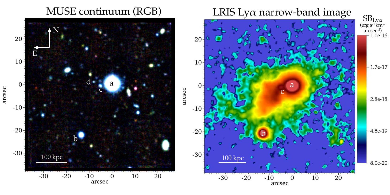
Figure 1: Left panel: reconstructed three-colour image of the final 9 hour exposure MUSE datacube centered on the Slug nebula. This image has been obtained by collapsing the cube in the wavelength dimension in three different pseudo-broad-bands: i) “blue” ($4875\mathrm{\AA}-6125\mathrm{\AA}$), ii) “green” ($6125\mathrm{\AA}-7375\mathrm{\AA}$), iii) “red” ($7375\mathrm{\AA}-8625\mathrm{\AA}$). The bright quasar UM287 ($g\simeq 17.5$ AB) and its much fainter quasar companion ($g\simeq 23$ AB) are labelled, respectively as “a” and “b” in the figure. Two of the brightest continuum sources embedded in the nebula are labelled as “c” and “d” (this is the same nomenclature as used in Leibler et al. 2018). Note that the color-scale is highly saturated in order to better visualise the faintest emission. Right panel: Ly$\alpha$ narrow-band image (reproduced from Cantalupo et al. 2014) of the same field of view as presented in the left panel. In addition to the quasar “a” and “b”, source “c” also shows the presence of enhanced Ly$\alpha$ emission with respect to the extended nebula. See text for a detailed discussion of the properties of these sources.

2.3 Cube combination

After applying CubeFix and CubeSharp to each individual exposure, a first combined cube is obtained using an average sigma clipping method (CubeCombine tool). This first cube is then used to mask and remove continuum sources in the second iteration of CubeFix and CubeSharp. After this iteration, the final cube is obtained with the same method as above. The final, combined cube has a 1$\sigma$ noise level of about $10^{-19}$ erg s^-1 cm^-2 arcsec^-2 per layer in an aperture of 1 arcsec² at 5300$\mathrm{\AA}$, around the expected wavelength of the Slug He ii emission.

In the left panel of Fig.1, we show an RGB reconstructed image obtained by collapsing the cube in the wavelength dimension in three different pseudo-broad-bands: i) “blue” ($4875\mathrm{\AA}-6125\mathrm{\AA}$), ii) ”green” ($6125\mathrm{\AA}-7375\mathrm{\AA}$), iii) ”red” ($7375\mathrm{\AA}-8625\mathrm{\AA}$), and by combining them into a single image. The 1$\sigma$ continuum noise levels in an aperture of 1 arcsec² are $0.33$, $0.27$, $0.33$ in units of $10^{-20}$ erg s^-1 cm^-2 arcsec^-2 $\mathrm{\AA}$ for the “blue”, “green” and “red” pseudo-broad-bands, respectively (these noise levels corresponds to AB magnitudes of about 30.1, 29.9, and 29.3 for the same bands). The bright quasar UM287 ($g\simeq 17.5$ AB) and its much fainter quasar companion ($g\simeq 23$ AB) are labelled, respectively as “a” and “b” in the figure. Two of the brightest continuum sources embedded in the nebula are labelled as “c” and “d” (this is the same nomenclature as used in Leibler et al. (2018). Source “c” shows also associated compact Ly$\alpha$ emission (see the right panel of Fig.1). In section 3.7, we will discuss the properties of these sources in detail.

3 Analysis and Results

Before the extraction analysis of possible extended emission line associated with the Slug, we subtracted both the main quasar (UM287) PSF and continuum from all the remaining sources, as described below.

3.1 QSO PSF subtraction

Quasar PSF subtraction is necessary in order to disentangle extended line emission from the line emission associated with the quasar broad line region. Although UM287 does not show $\text{He\,{ii}}\lambda 1640$ in emission, we choose to perform the quasar PSF subtraction on the whole available wavelength range to help the possible detection of other extended emission lines such as, C iv or C iii that are also present in the quasar spectrum. As for other MUSE quasar observations (both GTO and for several other GO programs) PSF subtraction was obtained with CubePSFSub (also part of the CubExtractor package) based on an empirical PSF reconstruction method (see also Husemann et al. 2013 for a similar algorithm). In particular, CubePSFSub uses pseudo-broad-band images of the quasar and its surroundings and rescales them at each layer under the assumption that the central pixel(s) in the PSF are dominated by the quasar broad line region. Then the reconstructed PSF is subtracted from each layer. For our analysis, we used a spectral width of 150 layers for the pseudo-broad-bands images. We found that this value provided a good compromise between capturing wavelength PSF variations and obtaining a good signal-to-noise ratio for each reconstructed PSF. We limited the PSF corrected area to a maximum distance of about 5” from the quasar to avoid nearby continuum sources (see Fig.1) from compromising the reliability of our empirically reconstructed PSF. To avoid that the empirically reconstructed PSF could be affected by extended nebular emission (producing over subtraction), we do not include the range of layers where extended emission is expected. Because, we do not know a priori in which layers extended emission may be present, we run CubePSFSub iteratively, increasing the numbers of masked layers until we obtain a PSF-subtracted spectrum that has no negative values at the edge of any detectable, residual emission line. In particular, in the case of $\text{He\,{ii}}\lambda 1640$ the masked layers range between the number 504 and 516 in the datacube (corresponding to the wavelength range 5380$\mathrm{\AA}-5395\mathrm{\AA}$). We note that the continuum levels of UM287 at the expected wavelength range of $\text{He\,{ii}}\lambda 1640$ are in any case negligible with respect to the sky-background noise at any distance similar or larger than the position of “source c” (see, e.g., the left panel of Fig.1). Therefore, including the PSF subtraction procedure at the $\text{He\,{ii}}\lambda 1640$ wavelength before continuum subtraction (as described below) does not have any noticeable effects on the results presented in this work.

3.2 Continuum subtraction

Continuum subtraction was then performed with CubeBKGSub (also part of the CubExtractor package) by means of median filtering, spaxel by spaxel, along the spectral dimension using a bin size of 40 pixel and by further smoothing the result across four neighbouring bins. Also in this case, spectral regions with signs of extended line emission were masked before performing the median filtering. In particular, in the case of $\text{He\,{ii}}\lambda 1640$ we masked every layer between the number 504 and 516 in the datacube (corresponding to the wavelength range 5380$\mathrm{\AA}-5395\mathrm{\AA}$) as performed during PSF subtraction.

Finally, we divided the cube into subcubes with a spectral width of about 63$\mathrm{\AA}$ (50 layers) around the expected wavelengths of the He ii, C iv, and C iii emission, i.e., around 5380$\mathrm{\AA}$, 5080$\mathrm{\AA}$, and 6250$\mathrm{\AA}$, respectively.

3.3 Three-dimensional signal extraction with CubExtractor

In order to take full advantage of the sensitivity and capabilities of an integral-field-spectrograph such as MUSE, three-dimensional analysis and extraction of the signal is essential. Intrinsically narrow lines such as the non-resonant $\text{He\,{ii}}\lambda 1640$ can be detected to very low levels by integrating over a small number of layers. On the other hand, large velocity shifts due to kinematics, Hubble flow or radiative transfer effects (in the case of resonant lines) could shift narrow emission lines across many spectral layers in different spatial locations. A single (or a series) of pseudo-narrow bands would therefore either be non-efficient in producing the highest possible signal-to-noise ratio from the datacube or missing part of the signal.

In order to overcome these limitations, we have developed a new three-dimensional extraction and analysis tool called CubExtractor (CubEx in short) that will be presented in detail in a separate paper (Cantalupo, in prep.). In short, CubEx performs extraction, detection and (simple) photometry of sources with arbitrary spatial and spectral shapes directly within datacubes using an efficient connected labeling component algorithm with union finding based on classical binary image analysis, similar to the one used by SExtractor (Bertin & Arnouts, 1996), but extended to 3D (see e.g., Shapiro & Stockman, Computer Vision, Mar 2000). Datacubes can be filtered (smoothed) with three-dimensional gaussian filters before extraction. Then datacube elements, called ”voxels”, are selected if their (smoothed) flux is above a user-selected signal-to-noise threshold with respect to the associated variance datacube. Finally, selected voxels are grouped together within objects that are discarded if their number of voxels is below a user-defined threshold. CubEx produces both catalogues of objects (including all astrometric, photometric and spectroscopic information) and datacubes in FITS format, including: i) “segmentation cubes” that can be used to perform further analysis (see below) and, ii) three-dimensional signal-to-noise cubes of the detected objects that can be visualised in three-dimensions with several public visualization softwares (e.g., VisIt).

3.4 Detection of extended He ii emission

We run CubEx on the subcube centered on the expected He ii emission with the following parameters: i) automatic rescaling of the pipeline propagated variance, ii) smoothing in the spatial and spectral dimension with a gaussian kernel of radius of 0.4” and 1.25$\mathrm{\AA}$ respectively, iii) a set of signal-to-noise (SNR) threshold ranging from 2 to 2.5, iv) a set of minimum number of connected voxels ranging from 500 to 5000. In all cases, we detected at least one extended source with more than 5000 connected voxels above a SNR threshold of 2.5. This source - that we call ”region c” - is located within part of the area covered by the Slug Ly$\alpha$ emission and, in particular, overlaps with sources “c” and “d” (see Fig.2). However, it does not cover the area occupied by the brightest Ly$\alpha$ emission - that we call “bright tail” - that extends south of source “c” by about 8” (see the right panel in Fig.1) at any explored SNR levels. This result does not change if we modify our spatial smoothing radius or do not perform smoothing in the spectral direction. The other detected source is the spatially compact but spectrally broader He ii emission associated with the broad-line-region of faint quasar “b” (not shown in Fig.2 ) while there is no clear detection within 2” of quasar “a”. Moreover, we have no information on the presence of nebular Ly$\alpha$ emission in this region because of the difficulties of removing the quasar PSF from the LRIS narrow-band imaging . For these reasons, we cannot reliably constrain the He ii/Ly$\alpha$ ratio within a few arcsec from quasar “a” and we will not consider this region in our discussion. In section 3.6 we estimate an upper limit to the possible contribution of the quasar Ly$\alpha$ emission PSF to the regions of interest in this work. Other, much smaller objects that appeared at low SNR thresholds are likely spurious given their morphology. To be conservative, we used in the rest of the He ii analysis of the “region c” the segmentation cube obtained by CubEx with a SNR threshold of 2.5.

In Fig. 2, we show the “optimally extracted” image of the detected He ii emission obtained by integrating along the spectral direction the SB of all the voxels associated with this source in the CubEx segmentation cube. These voxels are contained within the overlaid dotted contour. Outside of these contours (where no voxels are associated with the detected emission) we show for comparison the SB of the voxels in a single layer close to the central wavelength of the detected emission. Before spectral integration, a spatial smoothing with size of 0.8” has been applied to improve the visualisation. We stress that the purpose of this optimally extracted image (obtained with the tool Cube2Im) is to maximise the signal to noise ratio of the detection rather than the flux. However, by growing the size of the spectral region used for the integration, we have verified that the measured flux in the optimally extracted image can be considered a good approximation to the total flux within the measurement errors. This is likely due to the fact that we are smoothing also in the spectral direction and that the line is spectrally narrow as discussed in section 3.5. We note that the brightest He ii emission - approaching a SB close to 10^-17 erg s^-1 cm^-2 arcsec^-2 - is located in correspondence of the compact source “c”. The region above a SB of about 10^-18 erg s^-1 cm^-2 arcsec^-2 (coloured yellow in the figure) extends by about 5” (or about 40 kpc) in the direction of source “d”. The overall extension of the detected region approaches 12”, i.e., about 100 kpc. Below but still connected with this region there is a “faint tail” of emission detected with SNR between 2.5 and 4. Because the significance of this emission is lower, to be conservative we will focus in our discussion on the high SNR part of the emission (“region c”).

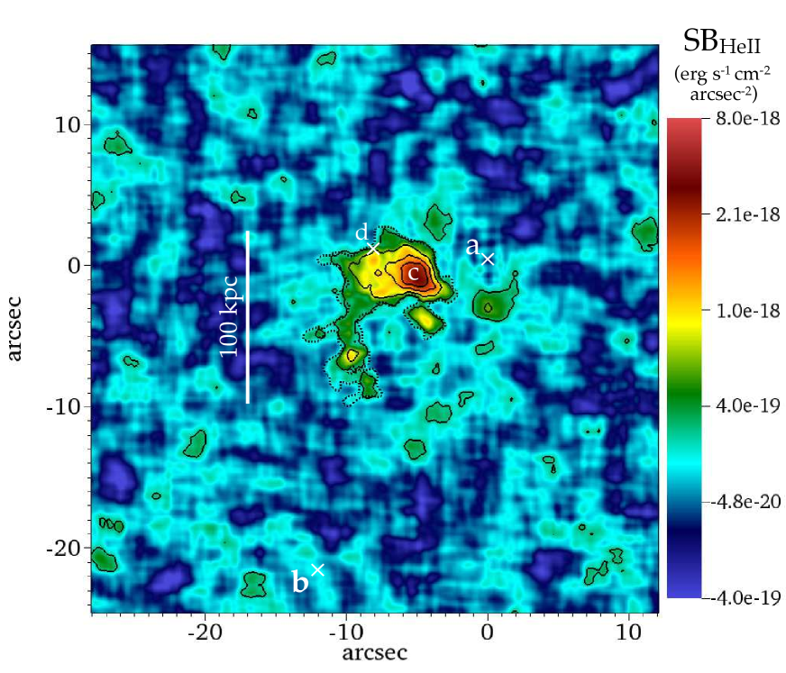
Figure 2: “Optimally extracted” image of the detected He ii emission from the Slug nebula. This image has been obtained by integrating along the spectral direction the SB of all the voxels associated with this source in the CubEx “segmentation cube” (see text for details). These voxels are contained within the overlaid dotted contour. Outside of these contours (where no voxels are associated with the detected emission) we show for comparison the SB of the voxels in a single layer close to the central wavelength of the detected emission. Before spectral integration, a spatial smoothing with size of 0.8” has been applied to improve visualisation. Solid contours indicate SNR levels of 2, 4, 6, and 8. The positions of quasars “a”, “b”, and sources “c” and “d” are indicated in the figure. The brightest He ii emission - approaching a SB close to 10^-17 erg s^-1 cm^-2 arcsec^-2 - is located in correspondence of the compact source “c”. The region above a SB of about 10^-18 erg s^-1 cm^-2 arcsec^-2 or SNR$>$4 (third solid contour line around source “c”) covers a projected area of about 6”$\times$3.5” (or about 50$\times$30 physical kpc). We refer to this region as “region c” in the text (see also Fig.3)

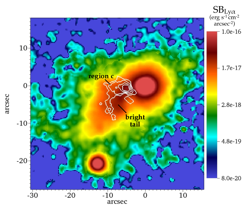
Figure 3: SNR contours of the detected He ii emission (solid white lines; see Fig.2) overlaid on the Ly$\alpha$ narrow-band image presented in right panel of Fig.1. There is little correspondence between the location of the brightest Ly$\alpha$ emission (that we call ”bright tail”, roughly centred at position $\Delta x=-7$” and $\Delta y=-5$” and labeled in the figure; we will use the Ly$\alpha$ surface brightness at this position in our calculations of line ratios for the “bright tail” ) and the majority of the He ii emission. The exception is the position occupied by the compact source “c”. Indeed, the He ii emitting region seems to avoid the ”bright tail”.

In Fig.3, we overlay the SNR contours of the detected He ii emission on the Ly$\alpha$ image for a more direct comparison. These contours have been obtained by propagating, for each spaxel, the estimated (and rescaled) variance from the pipeline (see section 3.4) taking into account the numbers of layers that contribute to the “optimally extracted” image in that spatial position (see also Borisova et al. 2016). As is clear from Fig. 3, there is very little correspondence between the location of the brightest Ly$\alpha$ emission (”bright tail”, labeled in the figure ) and the majority of the He ii emission, with the exception of the exact position occupied by the compact source “c”. Indeed, the He ii region seems to avoid the ”bright tail”. We will present in section 3.6 the implied line ratios and we will explore in detail the implications of this result in the discussion section.

3.5 Kinematic properties of the He ii emission

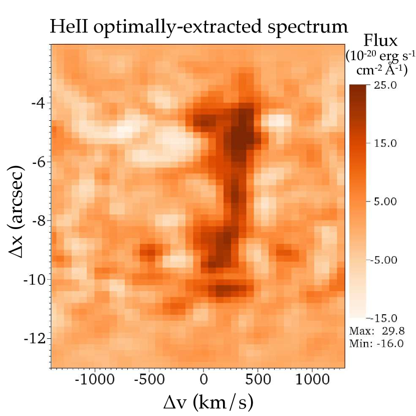
Figure 4: “Optimally extracted” two-dimensional spectrum of the detected He ii emission projected along the y-axis direction of Fig. 2. In particular, this spectrum has been obtained using the “segmentation cube” produced by CubEx (see text for details). Zero velocity corresponds to the CO systemic redshift of quasar “a” (i.e., z$=2.283$, DeCarli et al. in prep.) and the y-axis represents the projected distance (along the right ascension direction, i.e. the x-axis in the previous figures) in arcsec from “a”. For visualisation purposes, we have smoothed the cube in the spatial direction with a gaussian with radius 1 pixel (0.2”) before extracting the spectrum.

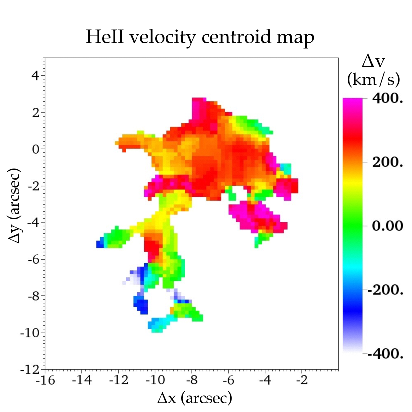
Figure 5: Two-dimensional map of the He ii emission velocity centroid, obtained as the first moment of the flux distribution of the voxels associated with the source detected by CubEx. The majority of the emission, located between $\Delta y=-3$”,$\Delta y=3$” (“region c”), shows a typical velocity shift between 200 and 300 km/s from the systemic redshift of quasar “a” and no evidence for ordered kinematical patterns such as, rotation, inflows or outflows. We note that the velocity shift of about 200km/s in the ”region c” is remarkably close the the one measured both in Ly$\alpha$ and H$\alpha$ emission at the same spatial location (see Leibler et al. 2018).

In Fig.4, we show the optimally extracted two-dimensional spectrum of the detected He ii emission projected along the y-axis direction. This spectrum has been obtained in the following way (automatically produced with the tool Cube2Im): i) we first calculated the spatial projection of the segmentation cube with the voxels associated with the detected object (“2d mask”; this region is indicated by the dotted contour in Fig.2); ii) we then used this 2d mask as a pseudo-aperture to calculate the spectrum integrating along the y-axis direction. In practice, this procedure maximises the signal-to-noise using a matched aperture shape. We notice that for each individual spatial position (vertical axis in the two-dimensional spectrum), the same number of voxels contribute to the flux, independent of the spectral position. However, the number of contributing voxels, and therefore the associated noise, may change between different spatial positions (as apparent in Fig.4). We used as zero-velocity the systemic redshift of the bright quasar “a” obtained by CO measurements (i.e., z$=2.283$, DeCarli et al. in prep.) and the y-axis represents the projected distance (along the right ascension direction, i.e. the x-axis in the previous figures) in arcsec from “a”.

The detected emission clearly stands-out along the spectral direction at high signal-to-noise levels between $\Delta x=-4$” and $\Delta x=-11$” and it is mostly centered around $\Delta v=300$km/s with coherent kinematics (at least in the region between $\Delta x=-4$” and $\Delta x=-8$”). Moreover, the emission appears very narrow in the spectral direction, despite the fact that we are integrating along about 4” in the y-spatial-direction. In particular, the FWHM in the central region ($\Delta x=-7$”) is only about 200 km/s, without deconvolution with the instrumental LSF, i.e., the line is barely resolved in our observation.

In Fig. 5, we show the two-dimensional map of the velocity centroid of the emission, obtained as the first moment of the flux distribution (using the tool Cube2Im) of the voxels associated with the detected source. As in Fig.4, the majority of the emission, located between $\Delta y=-3$” and $\Delta y=3$” (“region c”), shows a typical velocity shift between 200 and 300 km/s from the systemic redshift of quasar “a” with a remarkable coherence across distant spatial locations (with the exception of few regions associated with low signal-to-noise emission). At least at the spectral resolution of our observations, there is no evidence of ordered kinematical patterns such as, rotation, inflows or outflows. The lower signal-to-noise part of the emission located below $\Delta y=-3$” seems to show instead a velocity consistent with the systemic redshift of quasar “a” with large variations probably due to noise.

We note that the velocity shift of about 300km/s in this “region c” is remarkably close the the velocity shift measured both in Ly$\alpha$ and H$\alpha$ emission in the same spatial location (about 250 km/s for Ly$\alpha$ and about 400km/s for H$\alpha$; see Figs. 3 and 4 in Leibler et al. 2018). We also note that the Ly$\alpha$ emission appears broader (with a velocity dispersion of about 250km/s) and more asymmetric than the He ii emission, as expected in presence of radiative transfer effects.

3.6 He ii and Ly$\alpha$ line ratios

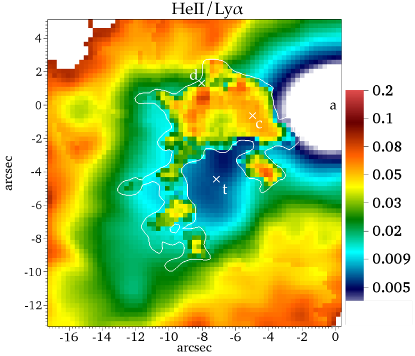
Figure 6: Two-dimensional He ii/Ly$\alpha$ ratio map. The region within the white contours represents measured values while the rest indicates 1$\sigma$ upper limits in an aperture of 0.8$\times$0.8 arcsec² and spectral width of 3.75$\mathrm{\AA}$. White colour indicates regions with no constraints. In section 3.6 we describe the detailed procedure used to obtain this map. The two adjacent and Ly$\alpha$-bright regions close to source “c” and the ”bright tail” immediately below show very different line ratios (or limits): the He ii-detected ”region c” shows He ii/Ly$\alpha$ up to 5% close to source “c” on average (increasing to about 8% close to source “d”) while the region immediately below that we call “bright tail” (i.e., around $\Delta x\simeq-7$” and $\Delta y\simeq-5$”; indicated by “t” in the figure ) shows 1$\sigma$ upper limits as low as 0.5%. As discussed in 3.6, we estimated that the quasar “a” Ly$\alpha$ PSF would at maximum increase the He ii/Ly$\alpha$ ratio by 25% close to source “c” and by less than 10% in the “bright tail” region. In section 4 we discuss the possible origin and implication of both the large gradients in the line ratio and the low measured values and upper limits.

In Fig. 6, we present the two-dimensional map of the measured (or 1$\sigma$ upper limit in an aperture of 0.8$\times$0.8 arcsec² and spectral width of 3.75$\mathrm{\AA}$) line ratio between He ii and Ly$\alpha$ emission combining our MUSE observations with our previous Ly$\alpha$ narrow-band image (Cantalupo et al., 2014). The measured values are enclosed within the white contour while the rest of the image represents 1$\sigma$ upper limit because of the lack of He ii detection in these regions. We note that the values and limits within a few arcsec from quasar “a” could be artificially lowered by the effects of the quasar Ly$\alpha$ PSF (that has not been removed in this image for the reasons mentioned in section 3.4). However, as discussed below, we estimated that quasar PSF effects would at maximum increase the He ii/Ly$\alpha$ ratio by 25% close to source “c” and by less than 10% in the “bright tail” region. We have obtained this two-dimensional line ratio map, using the following procedure: i) we smoothed the cube in the spatial directions with a boxcar with size 0.8” (4 spaxels), i.e. the FWHM of the measured PSF; ii) we obtained an optimally extracted image from the smoothed cube as described in section 3.4 (as discussed in the same section, this image represents the total He ii flux to within a good approximation); iii) we measured the average noise properties in the smoothed cube integrating within the three wavelength layers closer to the He ii emission, obtaining a 1$\sigma$ value of $1.69\times 10^{-19}$ erg s^-1 cm^-2 arcsec^-2 per smoothed pixel (equivalent to an aperture of 0.8”$\times$0.8”) and spectral width of 3.75$\mathrm{\AA}$; iv) we replaced each spaxel without detected He ii emission in the optimally extracted image with the 1$\sigma$ noise value as calculated above; v) we resampled the spatial scale of this image to match the spatial resolution of the LRIS Ly$\alpha$ NB image (i.e., 0.27” compared to the 0.2” of MUSE); vi) we extracted the Ly$\alpha$ emission from the LRIS image using CubEx and replaced pixels without detected emission with zeros; vii) we cut the LRIS image to match the astrometric properties of the MUSE optimally extracted image (using quasar “a” and “b” as the astrometric reference); viii) finally, we divided the two images by each other to obtain the measured He ii to Ly$\alpha$ line ratios (within the He ii detected region) or the line ratio 1$\sigma$ upper limit (in the region where He ii was not detected and Ly$\alpha$ is present).

The image presented in Fig. 6 quantifies the large difference in terms of line ratios between the two adjacent and Ly$\alpha$-bright regions close to source “c” and the ”bright tail” immediately below. In particular, the He ii-detected ”region c” shows He ii/Ly$\alpha$ up to 5% close to source “c” on average (increasing to about 8% 1” south of source “d”) while the region immediately below (i.e., around $\Delta x\simeq-7$” and $\Delta y\simeq-5$”, indicated by a “t”) shows 1$\sigma$ upper limits as low as 0.5%.

We note that these values can only be marginally affected by the lack of quasar Ly$\alpha$ PSF removal in our LRIS narrow-band image. In particular, we have estimated the maximum quasar Ly$\alpha$ PSF contribution by assuming that all the Ly$\alpha$ emission on the opposite side of the quasar position with respect to source “c” and the “bright tail” (i.e., emission at position $\Delta x>0$ in right-hand panel of Fig.1) is due to PSF effects. In this extreme hypothesis, we obtain that only about 25% of the Ly$\alpha$ emission around the location of source “c” and less than 10% of the Ly$\alpha$ emission in the bright tail could be affected by the quasar Ly$\alpha$ PSF. This effects would of course translate in an increased He ii/Ly$\alpha$ ratio of about 25% around source “c” and less than a 10% for the “bright tail”. We include these effects in the error bars associated with the measurements in these regions in the rest of this work.

Could the large gradient in line ratios be due to different techniques used to map He ii emission (i.e., integral-field spectroscopy) and Ly$\alpha$ (i.e., narrow band, with its limited transmission window)? The NB filter used on LRIS is centered on the Ly$\alpha$ wavelength corresponding to z=2.279 (Cantalupo et al., 2014), i.e. at a velocity separation of about $-350$ km/s from the quasar systemic redshift measured with the CO line that we are using as the reference throughout this paper. Therefore the Ly$\alpha$ emission associated with the “bright tail” is located exactly at the peak of the NB transmission window (see also Leibler et al. 2018). The FWHM of the filter corresponds to about 3000 km/s, therefore the filter transmission would be about half the peak value at a shift of about 1150 km/s with respect to the quasar “a” systemic redshift. Both the Ly$\alpha$ and the He ii emission detected from the “region c” extend up to a maximum velocity shift of about 500 km/s (see Fig.5 and Leibler et al. 2018). This is well within the high transmission region of the NB filter and therefore the Ly$\alpha$ SB of “region c” used in this paper could be underestimated by a factor less than two. This is much smaller than the factor of at least 10 difference in the observed line ratios. Therefore we conclude that the different observational techniques should not strongly affect our results. We will discuss the implications of the line ratios in terms of physical properties of the emitting gas in section 4.

3.7 Other emission lines

Using a similar procedure to the one applied to detect and extract extended He ii emission, we also searched for the presence of extended C iii and C iv emission (both doublets). The only location within the Slug where C iii and C iv are detected at significant levels is in correspondence of the exact position of the compact source “c”.

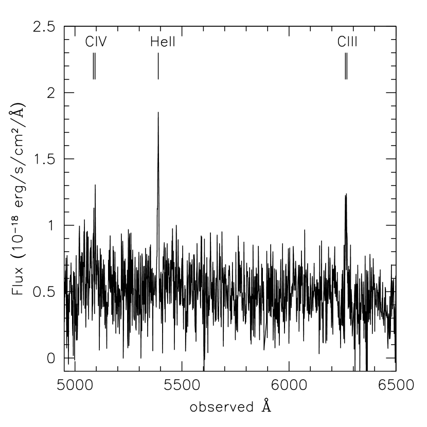
Figure 7: One-dimensional spectrum of the compact “source c” obtained within a circular aperture of diameter 1.6” (about twice the seeing FWHM) before continuum subtraction and after quasar PSF subtraction. The expected positions of C iv and C iii given the redshift obtained by the He ii emission are labeled in the figure. Both the C iv and C iii doublets are detected above an integrated signal to noise ratio of 3.

In Fig.7, we show the one-dimensional spectrum obtained by integrating within a circular aperture of diameter 1.6” (about twice the seeing FWHM) centered on source “c” before continuum subtraction and after quasar PSF subtraction. The expected positions of C iv and C iii given the redshift obtained by the He ii emission are labeled in the figure. Both C iv and C iii doublets are detected above an integrated signal to noise ratio of 3. Moreover, their redshifts are both exactly centered, within the measurement errors, on the systemic redshift inferred by the He ii line. As for He ii, both C iii and C iv are very narrow and marginally resolved spectroscopically. However, the detected signal to noise is too low in this case for a kinematic analysis. After continuum subtraction, both C iii and C iv have about half of the flux of the He ii line within the same photometric aperture.

The continuum has an observed flux density of about 5$\times 10^{-19}$ erg s^-1 cm^-2 $\mathrm{\AA}$ at 5000$\mathrm{\AA}$ (observed) and a UV-slope of about $\beta=-2.2$ (estimated from the spectrum between the rest-frame region 1670$\mathrm{\AA}$ to 2280$\mathrm{\AA}$) if the spectrum is approximated with a power-law defined as $f_{\lambda}\propto\lambda^{\beta}$. This value of $\beta$ would correspond to a extremely modest dust attenuation of $E(B-V)\sim 0-0.04$ (following Bouwens et al. 2014). For a starburst with an age between 10 and 250 Myr, the observed flux and $E(B-V)$ would imply a modest star formation rate ranging between 2 and 6 solar masses per year (e.g., Otí-Floranes & Mas-Hesse 2010).

In addition to the location of source “c” we have found some very tentative evidence (between 1 and 2 $\sigma$ confidence levels) for the presence of extended C iii at the spatial location of the “bright tail” and for the presence of extended C iv in the “region c” after large spatial smoothing ($>5"$ in size) in a small range of wavelength layers around the expected position. Because of the large uncertainty of these possible detections, we leave further analysis to future work. In particular, either deeper data or more specific tools for the extraction of extended line emission at very low SNR would be needed.

4 Discussion

We now focus our attention on the following questions: i) what is the origin of the large variations in both the Slug He ii emission flux and the He ii/Ly$\alpha$ ratio across adjacent regions in the plane of the sky (see Figs. 2 and 6)? ii) what constraints can we derive on the gas density distribution from the absolute values (or limit) of the He ii/Ly$\alpha$ ratios?

We will start by examining the effect of limited spatial resolution on the measured line emission ratios produced by two different ions for a broad probability distribution function (PDF) of gas densities. We will then discriminate between different physical scenarios for the origin of both Ly$\alpha$ and He ii emission (or lack thereof) and the large He ii/Ly$\alpha$ ratio variations. In particular, we will show that our results are best explained by fluorescent recombination radiation produced by regions that are located about 1 Mpc from the quasar along our line of sight. Finally, we will show that at least the brightest part of the Slug should be associated with a very broad cold gas density distribution that, if represented by a lognormal, would imply dispersions as high as the one expected in the Interstellar Medium (ISM) of galaxies (see e.g., Elmegreen, 2002). Finally, we will put our result in the context of other giant Ly$\alpha$ nebulae discovered around type-I and type-II AGN (mostly radio-galaxies).

4.1 Observed line ratios and gas density distribution

In this section, we emphasise that, when the gas density distribution within the photometric and spectroscopic aperture is inhomogeneous (as expected), the “observed” line ratio (e.g., $\langle F_{\rm{HeII}}\rangle/\langle F_{\rm{Ly\alpha}}\rangle$ as defined below) can be very different than the average “intrinsic” line ratio (e.g., $\langle F_{\rm{HeII}}/F_{\rm{Ly\alpha}}\rangle$) that would result from the knowledge of local densities in every point in space. In particular, this applies to all line emission that results from two-body processes (including, e.g., recombinations and collisional excitations) because their emission scales as density squared.

For instance, the “measured” He ii/Ly$\alpha$ line ratio produced by recombination processes (in absence of dust and radiative transfer effects) is defined, from an observational point of view, as:

$$\frac{<F_{\rm{HeII}}>}{<F_{\rm{Ly\alpha}}>}=\frac{h\nu_{\rm{HeII}}}{h\nu_{\rm{Ly\alpha}}}\frac{\alpha_{\rm{HeII}}^{\rm{eff}}(T)}{\alpha_{\rm{Ly\alpha}}^{\rm{eff}}(T)}\frac{<n_{e}n_{\rm{HeIII}}>}{<n_{e}n_{p}>}\ ,$$ (1)

where the average (indicated by the symbols “$<>$”) is performed over the photometric and spectroscopic aperture or, analogously, within the spatial and spectral resolution element (and captures the idea that the flux is an integrated measurement). The temperature-dependent effective recombination coefficients for the $\text{He\,{ii}}\lambda 1640$ and Ly$\alpha$ line are indicated by $\alpha_{\rm{HeII}}^{\rm{eff}}$ and $\alpha_{\rm{Ly\alpha}}^{\rm{eff}}$, respectively . In eq.1, we have assumed that the emitting gas within the photometric and spectroscopic aperture has a constant temperature. This is a reasonable approximation for photoionized and metal poor gas in the low-density limit ($n<10^{4}$ cm^-3), if in thermal equilibrium (e.g., Osterbrock 1989). Substituting the following expressions that assume primordial helium abundance and neglecting the small contribution of ionised helium to the electron density (up to a factor of about 1.2):

$$\begin{split}n_{\rm{HeIII}}&=0.087n_{\rm{H}}x_{\rm{HeIII}}\ ,\\ n_{p}&\equiv n_{\rm{H}}x_{\rm{HII}}\ ,\\ n_{e}&\simeq n_{\rm{H}}x_{\rm{HII}}\ ,\end{split}$$ (2)

we obtain:

$$\frac{<F_{\rm{HeII}}>}{<F_{\rm{Ly\alpha}}>}\simeq R_{0}(T)\frac{<n_{\rm{H}}^{2}x_{\rm{HeIII}}x_{\rm{HII}}>}{<n_{\rm{H}}^{2}x_{\rm{HII}}^{2}>}\ ,$$ (3)

where:

$$R_{0}(T)\equiv 0.087\frac{\nu_{\rm{HeII}}\alpha_{\rm{HeII}}^{\rm{eff}}(T)}{\nu_{\rm{Ly\alpha}}\alpha_{\rm{Ly\alpha}}^{\rm{eff}}(T)}\ .$$ (4)

Note that, for a temperature of $T=2\times 10^{4}$K, $R_{0}\simeq 0.23$ and $R_{0}\simeq 0.3$ for Case A and Case B, respectively.

Equation 3 can be simplified further assuming that the hydrogen is mostly ionised (i.e., $x_{\rm{HII}}\simeq 1$), as will typically be the case for the Slug nebula up to very high densities and large distances as we will show below, obtaining:

$$\begin{split}\frac{<F_{\rm{HeII}}>}{<F_{\rm{Ly\alpha}}>}\simeq R_{0}(T)\frac{<n_{\rm{H}}^{2}x_{\rm{HeIII}}>}{<n_{\rm{H}}^{2}>}\\ =R_{0}(T)\frac{\int_{V}x_{\rm{HeIII}}n_{\rm{H}}^{2}dV}{\int_{V}n_{\rm{H}}^{2}dV}\ ,\end{split}$$ (5)

where $V$ denotes the volume given by the photometric aperture (or spatial resolution element) and the spectral integration window. The expression above can be rewritten in terms of the density distribution function $p(n)$ as:

$$\frac{<F_{\rm{HeII}}>}{<F_{\rm{Ly\alpha}}>}\simeq R_{0}(T)\frac{\int x_{\rm{HeIII}}n_{\rm{H}}^{2}p(n_{\rm{H}})d{n_{\rm{H}}}}{\int n_{\rm{H}}^{2}p(n_{\rm{H}})d{n_{\rm{H}}}}\ ,$$ (6)

As is clear from the expressions above, the “measured” He ii/Ly$\alpha$ ratio for recombination radiation for highly ionised hydrogen gas will scale with the average fraction of doubly ionised helium, $x_{\rm{HeIII}}$, weighted by the gas density squared. We note that $x_{\rm{HeIII}}$ is in general a function of density, incident flux above 4 Rydberg (i.e. ionization parameter) and temperature. However, at a given distance from the quasar, the incident flux and temperature (due to photo-heating) will be fixed or within a limited range and therefore $x_{\rm{HeIII}}$ would mainly depend on density.

There is only one case in which the “measured” line ratio as defined above is equal to the average “intrinsic” one (e.g., $\langle F_{\rm{HeII}}/F_{\rm{Ly\alpha}}\rangle$), that is when $p(n_{\rm{H}})$ is a delta function. For any other density distribution, instead, the “measured” line ratio will be always smaller than the “intrinsic” value because $x_{\rm{HeIII}}$ decreases at higher densities and because of the $n_{\rm{H}}^{2}$ weighting.

When both hydrogen and helium are highly ionised, both the “measured” and “intrinsic” line ratios will tend to the maximum value $R_{0}(T)$ that is indeed independent of density. It is interesting to note that our measured He ii/Ly$\alpha$ ratio both in the “region c” ($\simeq 0.05$) and the upper limit in the “bright tail” ($\simeq 0.006$ at the 1$\sigma$ level) are significantly below $R_{0}(T)$ around temperatures of a few times $10^{4}$ K for both Case A ($\simeq 0.23$) and Case B($\simeq 0.3$). This is suggesting that helium cannot be significantly doubly ionised (see also Arrigoni Battaia et al. 2015) Moreover, as we will see below in detail, the “measured” line ratio in our case is low enough to provide a strong constraint on the clumpiness of the gas density distribution for the recombination scenario.

4.2 On the origin of the large He ii/Ly$\alpha$ gradient

In view of the discussion above, the possible origin of the strong “measured” line ratio variation across nearby spatial location within the Slug nebula include: i) a variation in Ly$\alpha$ emission mechanism, e.g. recombination versus quasar broad-line-region scattering, ii) quasar emission variability (in time, opening angle and spectral properties), iii) ionisation due to different sources than quasar “a”, iv) different density distribution, v) different physical distances.

The first possibility is readily excluded by the detection of H$\alpha$ emission from the “bright tail” of the Slug by Leibler et al. (2018), i.e. from the same region where He ii is not detected and the measured He ii/Ly$\alpha$ upper limit is the lowest. In particular, the relatively large H$\alpha$ emission measured from this region exclude any significant contribution to the Ly$\alpha$ emission from scattering of the quasar broad line regions photons.

Another possibility is that the “bright tail” region without detected He ii emission does not receive a significant amount of photons above 4 Rydberg from quasar “a” due to, e.g. time variability effects (see e.g., Peterson et al. 2004, Vanden Berk et al. 2004, Ross et al. 2018 and references therein), quasar partial obscuration (see e.g., Elvis 2000, Dong et al. 2005, Gaskell & Harrington 2018 and references therein) or because of possible spectral “hardness” variations along different directions . Although this scenario would easily explain even a extremely low He ii/Ly$\alpha$ ratio and strong spatial gradients, it would be very difficult to reconcile the fact that the line ratio variations seem to correlate extremely well with kinematical variations in terms of Ly$\alpha$ line centroid (e.g., Leibler et al. 2018).

The presence of source “c” within the He ii detected region could hint at the possibility that different sources are responsible for the ionisation of different part of the nebula, particularly if source “c” harbours an Active Galactic Nucleus (AGN). If this source were fully ionizing both hydrogen and helium, we would have expected to see a line ratio approaching 0.3 (Case B) or 0.23 (Case A) as discussed in section 4.1. However, the measured line ratio is much below these values. Therefore, if source “c” is responsible for the photoionization of “region c” one would have expected to see variations in the He ii/Ly$\alpha$ ratio close to the location of this source. This is because ionisation effects should scale as $1/r^{2}$ (see below for details). However, as shown in Fig.6, the line ratio is rather constant around the location of source “c”. This would require a fine tuned variation in the gas density distribution to balance the varying flux in order to produce the absence of line ratio variations across the location of source “c”. We consider this possibility unlikely. Moreover, both from the infrared observation of Leibler et al. (2018) and from the narrowness of the rest-frame UV emission lines it is very unlikely that source “c” could harbor an AGN bright enough to produce both the extended He ii and Ly$\alpha$ emission (the same applies considering the relatively low SFR of this sources derived in the previous sections). The most likely hypothesis therefore is that the 4 Rydberg “illumination” is coming from the more distant but much brighter quasar “a”. Similarly, the absence of detectable bright continuum sources in the “bright tail” region (see Fig.1) suggests that ultra-luminous quasar “a” is the most likely source of “illumination” for this region. The only other securely detected AGN in this field, the quasar companion “b”, is more than 5 magnitudes fainter than quasar “a” and even more distant in projected space (although there is large uncertainty in redshift for this quasar) from both “region c” and the “bright tail” with respect to the other possible sources considered here. Finally, we notice that including any possible additional contribution to the helium ionising flux from quasar “b” or even source “c” with respect to quasar “a” would strengthen the requirement for large gas densities as discussed below and in section 4.3.

By excluding the scenarios above as the least plausible we are left with the possibilities that the line ratio variations are due to either gas density distribution variations (as discussed in 4.1) or different physical distances, or both. On this regard, it is important to notice that the gradient in the He ii/Ly$\alpha$ ratio is mostly driven by a strong variation in the He ii emission. Indeed the Ly$\alpha$ SB of the “region c” and “bright tail” are very similar. In the plausible assumption that the hydrogen is highly ionised in both regions, as we will demonstrate later, any density variation across the two regions should produce a significant difference in Ly$\alpha$ SB. For instance, in the highly simplified case in which the emitting gas density distribution is constant, the Ly$\alpha$ emission from recombination radiation would scale as the gas density squared while the line ratio would only scale about linearly with density, as discussed below. In more general cases, discussed in the next section, we will show that indeed the Ly$\alpha$ SB is more sensitive to density variation than the line ratio.

The most likely hypothesis therefore is that different physical distances of the two regions from the quasar produce the lack of detectable He ii emission that results in the strong observed gradient in the He ii/Ly$\alpha$ ratio. This suggestion is reinforced by the fact that the He ii/Ly$\alpha$ gradient arises exactly at the spatial location where a strong and abrupt Ly$\alpha$ velocity shift is present (see e.g., Leibler et al. 2018) In particular, the velocity shift between the “bright tail” and “region c” is as large as 900 km/s as measured from Ly$\alpha$, H$\alpha$ and He ii emission. This is much larger than the virial velocity of a dark matter halo with mass of about $10^{13}$ solar masses at this redshift (about 450 km/s). If completely due to Hubble flow, this velocity shift would correspond to physical distances as large as 4 Mpc. Note that the quasar “a” systemic redshift is located in between these two regions (-350 km/s from “region c” and +650 km/s from the “bright tail”). However, because peculiar velocities as large as a few hundreds of km/s are expected in such an environment, it is difficult to firmly establish if the quasar is physically between these two regions along our line of sight or in the background.

In the next section, we will evaluate in detail the expected line ratios for a given density distribution function and distance from the quasar. However, it is instructive here to consider the simplest case in which the emitting gas density distribution is constant (i.e. is a delta function $p(n)=\delta(n-n_{0})$) and equal for both regions. In this case, we can simply evaluate in which situations the different line ratios could be explained just in terms of different relative distances from the quasar. Assuming once again that hydrogen is highly ionised (implying both $x_{\rm{HI}}\simeq 0$ and $x_{\rm{HeI}}\simeq 0$), it is easy to show that:

$$x_{\rm{HeIII}}=\frac{\Gamma_{\rm{HeII}}}{\Gamma_{\rm{HeII}}+n_{0}\alpha_{\rm{HeIII}}}\ ,$$ (7)

and, therefore using eq. 5 that:

$$\frac{LR^{c}}{LR^{tail}}\simeq\frac{\Gamma_{\rm{HeII}}^{c}}{\Gamma_{\rm{HeII}}^{tail}}\times\left(\frac{\Gamma_{\rm{HeII}}^{tail}+n_{0}\alpha_{\rm{HeIII}}}{\Gamma_{\rm{HeII}}^{c}+n_{0}\alpha_{\rm{HeIII}}}\right)\ ,$$ (8)

where $LR^{c}$ and $LR^{tail}$ represent the measured line ratio in “region c” and the “bright tail”, respectively, while $\Gamma_{\rm{HeII}}^{c}$ and $\Gamma_{\rm{HeII}}^{tail}$ are the corresponding He ii photoionisation rates in these regions. Finally, $\alpha_{\rm{HeIII}}$ denotes the temperature dependent He iiI recombination coefficient for which we use a value of $1.3\times 10^{-12}$ cm³ s^-1 at $T\sim 2\times 10^{4}$ K. Given the observed continuum luminosity of our quasar and a typical spectral profile in the extreme UV as in Lusso et al. (2015) the He ii photoionization rate is given by:

$$\Gamma_{\rm{HeII}}\simeq 9.2\times 10^{-12}\left(\frac{r}{500\rm{kpc}}\right)^{-2}\rm{s^{-1}}\ ,$$ (9)

where $r$ denotes the physical distance between the quasar and the gas cloud. When $\Gamma_{\rm{HeII}}^{c}/(n_{0}\alpha_{\rm{HeIII}})\ll 1$ (and similarly for the tail region), corresponding to, e.g., $n_{0}>7$ cm^-3 at $r=500$ kpc, equation 8 can be approximated as:

$$\frac{LR^{c}}{LR^{tail}}\simeq\frac{\Gamma_{\rm{HeII}}^{c}}{\Gamma_{\rm{HeII}}^{tail}}\ ,$$ (10)

implying that a gradient of about a factor of ten in the line ratio could be easily explained, in this simplified case, if the “bright tail” region is about three times more distant than the “region c” with respect to the quasar. For smaller values of $n_{0}$ this ratio of distances increases to a factor of about four when $\Gamma_{\rm{HeII}}^{c}/(n_{0}\alpha_{\rm{HeIII}})\sim 1$. In case a broad density distribution is used, the required ratio in relative distances can be again reduced to about a factor of three, even if the average density is much below the values discussed above, as we will see in the next section. It is interesting to note that this factor of three is totally consistent with the kinematical constraints discussed above.

Using similar arguments as before, it is simple to verify that if the two regions are placed at the same distance (and therefore they have the same $\Gamma_{\rm{HeII}}$), a factor of ten variation in the line ratio would imply a density ratio at least as high as this (assuming that the density distributions are delta functions). As mentioned above, this would therefore imply a change in the Ly$\alpha$ SB by a factor $n_{0}^{2}$, i.e. by a factor of at least 100, which is indeed not observed.

In this section, we have assumed that the hydrogen is mostly ionised. This is a reasonable assumption because the density values at which hydrogen becomes neutral are very large, given the expected large value of the hydrogen photoionisation rate for UM287 (obtained as above) in the conservative assumption that this is the only source of ionisation:

$$\Gamma_{\rm{HI}}\simeq 3.9\times 10^{-10}\left(\frac{r}{500\ \rm{kpc}}\right)^{-2}\rm{s^{-1}}\ .$$ (11)

Indeed, assuming a temperature of $2\times 10^{4}$ K and the case A recombination coefficient $\alpha_{\rm{HII}}\simeq 2.5\times 10^{-13}$ cm³ s^-1, the hydrogen will become mostly neutral above the following density:

$$n_{\mathrm{H}}^{\mathrm{HI,crit}}\simeq\frac{\Gamma_{\rm{HI}}}{\alpha_{\rm{HII}}}\simeq 1500\left(\frac{r}{500\ \rm{kpc}}\right)^{-2}\rm{cm^{-3}}.$$ (12)

As a comparison, the density for which He iii becomes He ii, as derived above, is about 200 times smaller:

$$n_{\mathrm{H}}^{\rm{HeII,crit}}\simeq\frac{\Gamma_{\rm{HeII}}}{\alpha_{\rm{HeIII}}}\simeq 7\left(\frac{r}{500\ \rm{kpc}}\right)^{-2}\rm{cm^{-3}}.$$ (13)

There is therefore a large range of densities at which hydrogen is still ionised while most of the doubly ionised helium is not present. In the next section, we will show the result of our full calculation that takes into account the proper ionised fraction at each density.

4.3 On the origin of the small He ii/Ly$\alpha$ values

In the previous section, we have discussed how the strong gradients in the He ii/Ly$\alpha$ ratio combined with kinematic information and the presence of H$\alpha$ emission, suggest that the “bright tail” regions should be at least three times more distant from the quasar “a” than “region c” (in the case of constant emitting gas density distribution). In this section, we explore which constraints on the (unresolved) emitting gas density distribution and absolute distances can be derived from the measured values (or limits) of the He ii/Ly$\alpha$ ratios. As in the previous section, we will make the plausible assumption that the main emission mechanism for both lines is recombination radiation and that scattering from the quasar broad line region is negligible (as implied by the detection of H$\alpha$ emission). Collisional excitation can be excluded for the $\text{He\,{ii}}\lambda 1640$ line, as it would require electron temperatures of about 10⁵ K that are difficult to produce for photo-ionised and dense gas, even for a quasar spectrum (that would range between $2-5\times 10^{4}$ K, e.g. Cantalupo et al. 2008). Collisionally-excited Ly$\alpha$ emission could be produced instead efficiently at the expected temperatures (e.g. Cantalupo et al. 2008) but the volume occupied by partially ionised dense gas, if present at all, will be negligible with respect to the ionized volume (see section 4.2). Finally, we will make the conservative assumption that quasar “a” is the only source of ionisation.

4.3.1 Maximum distance from quasar “a”

We have shown in section 4.1 that the “measured” line ratio can be very sensitive to the emitting gas density distribution within the photometric and spectroscopic aperture. In particular, we expect that a broader density distribution function at a fixed average density will produce lower line ratios. Any constraint on the density distribution would be however degenerate with the value of the photoionisation rate of He ii, that, in turn depends on the distance of the cloud. In particular, we expect that at larger distances, smaller densities would be required to produce a low line ratio. It is therefore important to derive some independent constraints on, e.g., the maximum distance at which the “bright tail” region could be placed, in order to derive meaningful constraints on its gas density distribution from the He ii/Ly$\alpha$ ratio.

Such constraints could be derived by the self-shielding limit for the Ly$\alpha$ fluorescent surface brightness produced by quasar “a” (e.g., Cantalupo et al. 2005). In this limit, reached when the total optical depth to hydrogen ionising photons becomes much larger than one, the expected emission is independent of local densities and depends only on the impinging ionising flux. In particular, using the observed luminosity of quasar “a” (UM287) and assuming the same spectrum as in the previous section, the maximum distance as a function of the observed Ly$\alpha$ SB will be (see also Arrigoni Battaia et al. 2015):

$$r_{\rm{max}}\simeq 1\ \rm{Mpc}\times\left(\frac{\rm{SB_{Ly\alpha,17}}}{2.25}\right)^{-0.5}\left(\frac{f_{\rm{C}}}{1.0}\right)^{0.5}\left(\frac{\Gamma^{\rm{act}}_{\rm{HI}}}{\Gamma_{\rm{HI}}^{\rm{obs}}}\right)^{0.5}$$ (14)

where $\rm{SB_{Ly\alpha,17}}$ is the observed Ly$\alpha$ SB in units of $10^{-17}\rm{erg\ s^{-1}\ cm^{-2}\ arcsec^{2}}$, $f_{\rm{C}}$ is the self-shielded gas covering fraction within the spatial resolution element, $\Gamma_{\rm{HI}}^{\rm{obs}}$ is the inferred photoionisation rate for UM287 using the currently observed quasar luminosity (along our line of sight), and $\Gamma^{\rm{act}}_{\rm{HI}}$ is the actual photoionization rate at the location of the optically thick gas. Note that both $f_{\rm{C}}$ and $\Gamma^{\rm{act}}_{\rm{HI}}$ could be uncertain within a factor of a few.

The observed Ly$\alpha$ SB in both the “bright tail” and “region c” is around $2.5\times 10^{-17}\rm{erg\ s^{-1}\ cm^{-2}\ arcsec^{2}}$ corresponding to a maximum distance of about 1 physical Mpc. This distance would be larger if the observed SB is decreased because of local radiative transfer effects or absorption along our line of sight. For similar reasons, the quoted Ly$\alpha$ SBs in the reminder of this section should be considered as upper limits. We also note that there is very little or no spatial overlap in the Ly$\alpha$ image between the “bright tail” and “region c” as they are very well separated in velocity space without signatures of double peaked emission (Leibler et al. 2018).

4.3.2 Delta function density distribution

Before moving to more general density distributions, it is interesting to consider again the extremely simplified case of the delta function $p(n)=\delta(n_{0})$ and to derive the minimum densities needed to explain the He ii/Ly$\alpha$ upper limits in the “bright tail” if placed at the maximum distance of 1 Mpc. Using the results of the previous section, a temperature of $T=2\times 10^{4}$K, and assuming conservatively the 2$\sigma$ upper limit of 0.012 for the He ii/Ly$\alpha$ ratio we derive a density of $n_{0}\simeq 30$ cm^-3 for Case A and $n_{0}\simeq 75$ cm^-3 for Case B (for both hydrogen and helium). As shown in the previous section, these densities would also explain the measured line ratio in “region c” if located at a distance of about 300 kpc from quasar “a”. The derived densities increase as the square root of the distance from the quasar and the values quoted above should be considered as an absolute minimum for a delta function density distribution of the (cold) emitting gas. Such high densities, combined with the observed Ly$\alpha$ SB would imply an extremely small volume filling factor of the order of $f_{V}\simeq 10^{-6}$, if each of the two regions has a thickness along our line of sight of about 100 kpc (see, e.g. equation 3 in Cantalupo 2017 ).

Unless these clouds are gravitationally bound, we expect that such high densities would be quickly dismantled in a short timescale: these clouds cannot be pressure confined because the hot gas surrounding them should have temperatures or densities that are at least one order of magnitude larger than what structure formation could reasonably provide. For instance, the virial temperature and densities of a 10¹³ M_⊙ dark matter halo at $z\simeq 2.3$ are expected to be around $3\times 10^{7}$ K and 10^-3 cm^-3, respectively. Therefore, even in the very unlikely hypothesis that both ”region c” and the ”bright tail region” are associated with such massive haloes, only gas clouds with densities of about 1.5 cm^-3 could be pressure confined. In order to confine gas clouds with a density of $n_{0}\simeq 30$ cm^-3 once photoionized by the quasar (and therefore at a temperature of about 2$\times 10^{4}$ K), we would require either a hot gas temperature of $6\times 10^{8}$ K or a hot gas density that is 20 times higher than the virial density. Alternatively, the temperature of the cold clouds should be initially much lower than 10³ K, implying that these clouds are in the process of photo-evaporating after being illuminated by the quasar. All these situation are problematic because they either require extreme properties for the confining hot gas or that the cold clouds are extremely short lived, with obvious implication for the observability of giant Ly$\alpha$ nebulae.

4.3.3 Log-normal density distribution

These problems can be solved by relaxing one of the extreme simplifications made above (and in general in other photo-ionisation models in the literature), i.e. that the emitting gas density distribution is a delta function. As demonstrated in section 4.1, a broad density distribution may decrease the “observed” line ratio by a large factor while keeping the same volume-averaged density. Broad density distributions are commonly observed in multiphase media like, e.g., the ISM of our galaxy (e.g. Myers, 1978). In particular, both simulations and observations suggest that gas densities in a globally stable and turbulent ISM is well fitted by a lognormal Probability Distribution Function (PDF) (e.g, Wada & Norman 2007 and references therein):

$$\mathrm{PDF}(n)dn=\frac{1}{\sqrt{2\pi}\sigma}\exp{\left[-\frac{[\mathrm{ln}(n/n_{1})]^{2}}{2\sigma^{2}}\right]}d\mathrm{ln}(n),$$ (15)

where $\sigma$ is the lognormal dispersion and $n_{1}$ is a characteristic density that is connected to the average volume density by the relation:

$$\langle n\rangle_{c}=n_{1}\exp{\frac{\sigma^{2}}{2}}.$$ (16)

Numerical studies suggested that a lognormal distribution is characteristic of isothermal, turbulent flow and that $\sigma$ is determined by the “one-dimensional Mach number ($M$)” of the turbulent motion following the relation: $e^{\sigma^{2}}\sim 1+3M^{2}/4$ (e.g., Padoan & Nordlund, 2002). Although a discussion of the origin of the gas density distribution in the ISM and its effect on the galactic star formation is clearly beyond the scope of this paper, we notice that a large value of $\sigma$ (e.g., $\sigma\sim 2.3$) has been suggested as a key requirement to reproduce the Schmidt-Kennicutt law (see e.g., Elmegreen, 2002; Wada & Norman, 2007).

In the remainder of this section, we use a lognormal density distribution as a first possible ansatz for the PDF of the emitting gas in the Slug nebula, with the assumption that some of the processes that may be responsible for the appearance of such a PDF in the ISM may be operating also in our case. Our main requirement is that the cold emitting gas is “on average” in pressure equilibrium with a hot confining medium, i.e. that the density averaged over the volume of the cold gas ($\langle n\rangle_{c}$) should be determined by the temperature and density of the confining hot gas. In this context, the broadness of the gas density distribution represents a perturbation on densities that could be caused by, e.g., turbulence, sounds waves, or other (unknown) processes that may act on both local or large scales. Examples of large-scale perturbation may be caused by gravitational accretion combined with hydrodynamical (e.g., Kelvin-Helmholtz) or thermal instabilities as we will discuss elsewhere (Vossberg, Cantalupo & Pezzulli, in prep.; see also Mandelker et al. 2016; Padnos et al. 2018; Ji et al. 2018). Because these density perturbations will be either highly over-pressured or under-pressured for large $\sigma$ we expect that they would dissipate quickly. Therefore, we expect that $\sigma$ will be reduced over time if the perturbation mechanism is not acting continuously or if the resulting structures do not become self-gravitating.

Our working hypothesis is that the confining hot gas is virialized within dark matter haloes that are part of the cosmic web around quasar “a”. The hot gas density is therefore fixed at about 200 times the average density of the universe at $z\simeq 2.3$, i.e., $n_{\rm{hot}}\simeq 1.4\times 10^{-3}$ cm^-3 and the temperature is assumed equal to the virial temperature of a given dark matter halo mass at this redshift. In turn, this temperature is related to the average density of the cold gas (assumed to be at a temperature of $2\times 10^{4}$ K) by the pressure-confinement condition discussed above. The other ingredients of our simple model are: i) the mass fraction of gas in the cold component within the virial radius ($f_{\rm{cold}}$) which we assume to be 10%, and ii) the size of the emitting region along the line of sight that we assume to be 100 kpc. Given the densities of the hot and cold components, this cold mass fraction translates into a given volume filling factor that determines the expected Ly$\alpha$ SB. We stress that the actual value of $f_{\rm{cold}}$ only affects the Ly$\alpha$ SB and that any increase in $f_{\rm{cold}}$ can be compensated by a smaller size of the emitting region along the line of sight, producing the same results.

The running parameters in the model are therefore: i) the average volume density of the cold gas component $\langle n\rangle_{c}$, ii) the log-normal dispersion $\sigma$, and iii) the distances of “region c” and the “bright tail” from quasar “a”. These four parameters will be fixed by the observed Ly$\alpha$ SB and the He ii/Ly$\alpha$ line ratios of both regions, under the assumption that they are characterised by the same density distributions. Given the assumption of “average” pressure equilibrium above, the masses of the hosting dark matter haloes of these structures will be directly linked to the average volume density of the cold gas $\langle n\rangle_{c}$.

In Fig. 8, we show the result of our photoionisation models for case B recombination emission (lines) compared to the observed Ly$\alpha$ SB and He/Ly$\alpha$ ratios for both the “region c” (black square; error bars include the maximum effect of the quasar Ly$\alpha$ PSF, see section 3.6) and “bright tail” (blue square, indicating the 2$\sigma$ upper limit; the upper error bar indicates the 3$\sigma$ upper limit; for simplicity, we use the 2$\sigma$ upper limit as a measured point for the line ratio). The predicted values have been obtained from eq. 1 by numerically solving the combined photoionization equilibrium equations for both hydrogen and helium in all their possible ionisation states at each density given by a lognormal distribution with dispersion $\sigma$ and average volume density $\langle n\rangle_{c}$. In particular, we show two sets of lines: the blue lines correspond to a distance of 900 kpc from quasar “a” (slightly below the maximum distance for hydrogen self-shielding) and the black lines correspond to a distance of 270kpc. For each set of lines we run our models with three different $\langle n\rangle_{c}$: i) $\langle n\rangle_{c}=0.02$ cm^-3, corresponding to a dark matter host halo M_h of about 10¹¹ M_⊙ (and volume filling factor of the cold emitting gas $f_{v}\simeq 8\times 10^{-3}$), ii) $\langle n\rangle_{c}=0.05$ cm^-3 (M${}_{h}\simeq 10^{11.5}$ M_⊙ and $f_{v}\simeq 3\times 10^{-3}$ ), and iii) $\langle n\rangle_{c}=0.1$ cm^-3 (M${}_{h}\simeq 10^{12.0}$ M_⊙ and $f_{v}\simeq 10^{-3}$ ). These average densities span a range of plausible halo masses for the host haloes. Finally, each point along the lines represent a different value of $\sigma$ and we overlay, for clarity, several coloured circles equally spaced with $\Delta\sigma=0.2$ at $\sigma$ values indicated by the color bar. The regions of parameter space that are not allowed because of the hydrogen self-shielding limit are shaded in grey. We note that the predicted Ly$\alpha$ SB scales linearly with the product of $f_{v}$ (determined by $\langle n\rangle_{c}$ and the cold mass fraction that we fixed to 10%) and the size of the emitting region along the line of sight, that we have assumed to be 100 kpc. However, the line ratio is of course independent of these parameters.

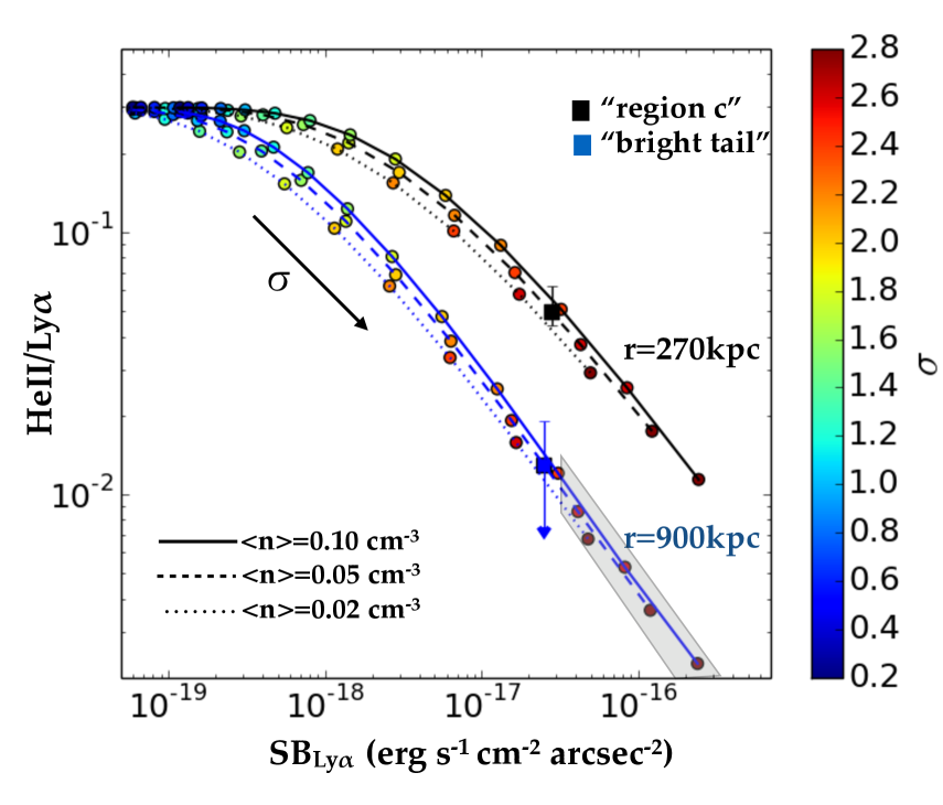
Figure 8: Results of our photoionisation models for case B recombination emission (lines) compared to the observed Ly$\alpha$ SB and He/Ly$\alpha$ ratios for both “region c” (black square; error bars include the maximum effect of the quasar Ly$\alpha$ PSF, see section 3.6) and “bright tail” (blue square, indicating the 2$\sigma$ upper limit; the upper error bar indicates the 3$\sigma$ upper limit; for simplicity, we use the 2$\sigma$ upper limit as a measured point for the line ratio), in the conservative assumption that quasar “a” is the only source of ionisation. The predicted values have been obtained from eq. 1 by numerically solving the combined photoinization equilibrium equations for both hydrogen and helium in all their possible ionisation states at each density given by a lognormal distribution with dispersion $\sigma$ and average volume density $\langle n\rangle_{c}$. Two sets of lines are shown depending on the cloud distance from quasar “a”: 900kpc (blue) and 270kpc (black). For each set of lines we run our models with three different $\langle n\rangle_{c}$: i) $\langle n\rangle_{c}=0.02$ cm^-3, corresponding to a dark matter host halo M_h of about 10¹¹ M_⊙ (and volume filling factor of the cold emitting gas $f_{v}\simeq 8\times 10^{-3}$), ii) $\langle n\rangle_{c}=0.05$ cm^-3 (M${}_{h}\simeq 10^{11.5}$ M_⊙ and $f_{v}\simeq 3\times 10^{-3}$ ), and iii) $\langle n\rangle_{c}=0.1$ cm^-3 (M${}_{h}\simeq 10^{12.0}$ M_⊙ and $f_{v}\simeq 10^{-3}$ ). Finally, each point in the lines represent a different value of $\sigma$ and we overlay several coloured circle equally spaced with $\Delta\sigma=0.2$ at $\sigma$ values indicated by the color bar. The regions of parameter space that are not allowed because of the hydrogen self-shielding limit are shaded in grey. The models reproduce the observed values (or limits) only for broad density distribution with $2.4<\sigma<2.7$ and only if the gas associated with the “bright tail” is located at large distances from the quasar “a”, close to the self-shielding limit of about 1 Mpc. We notice that, including any possible contribution to both hydrogen and helium ionizing radiation from other sources would require even broader gas density distributions and would move the self-shielding limit to even larger SB. See text for further discussion.

As clear from the figure and as expected from our discussion of the “observed” versus “intrinsic” line ratios, the broadness of the density distribution is the main factor driving the predicted line ratios to low values. In particular, no model is able to produce line ratios below 10% unless $\sigma>1.5$. Furthermore, large distances (close to the self-shielding limit for Case B recombination) are also required to explain the He ii/Ly$\alpha$ limit obtained for the “bright tail”. Line ratios are instead less sensitive to the value of $\langle n\rangle_{c}$. However, at a fixed distance, $\sigma$ and $\langle n\rangle_{c}$ are degenerate, in the sense that the observed line ratios and Ly$\alpha$ SB could be explained by a smaller $\sigma$ if $\langle n\rangle_{c}$ is higher. For instance, if the “bright tail” is at 900 kpc from quasar “a”, the upper limit on the line ratio and the measured Ly$\alpha$ SB could be explained by a lognormal density distribution with $2.4<\sigma<2.7$ for $(0.10\ \mathrm{cm^{-3}})>\langle n\rangle_{c}>(0.02\ \mathrm{cm^{-3}})$. As a reference, such values of $\sigma$ correspond to “internal” clumping factors ($C_{c}\equiv\langle n^{2}\rangle_{c}/\langle n\rangle_{c}^{2}$, that for a lognormal distribution is simply given by $C=\exp{(\sigma^{2})}$) $300\lesssim C_{c}\lesssim 1000$ for the cold component, in agreement with the estimated based on comparison with cosmological simulations for the Ly$\alpha$ SB discussed in Cantalupo et al. (2014). These values would also explain the measured line ratios and Ly$\alpha$ SB of the “region c” if placed at a distance of 270 kpc. As expected, the He ii/Ly$\alpha$ ratio and the Ly$\alpha$ SB are generally anticorrelated. In particular, at a fixed average density $\langle n\rangle_{c}$, the Ly$\alpha$ SB increases linearly with the ”internal” clumping factor $C=\exp{(\sigma^{2})}$. At the same time, larger values of $\sigma$ produce smaller He ii/Ly$\alpha$ ratios. This means that, if the Ly$\alpha$ SB in some region of Ly$\alpha$ nebulae is driven by large clumping factors then we necessarily expect low He ii/Ly$\alpha$ within the same regions.

We note that performing the calculation using the Case A effective and total recombination coefficients would require slighter smaller values of $\sigma$ at a fixed distance to obtain the same He ii/Ly$\alpha$ ratios, i.e. $\sigma\simeq 2.3$ instead of $\sigma\simeq 2.5$ for the “bright tail” for $\langle n\rangle_{c}=0.05$ cm^-3 (see Appendix). On the other hand, at a fixed $\sigma=2.5$ and $\langle n\rangle_{c}=0.05$ cm^-3, the Case A calculation produces He ii/Ly$\alpha$ ratios consistent with the $2\sigma$ upper limit of the “bright tail” for distances equal or larger than about 550 kpc instead of 900 kpc. For “region c” the required distance decreases to about 180 kpc (see Appendix). In all cases, however, a log-normal distribution with $\sigma>2.3$ is required to match the low He ii/Ly$\alpha$ ratios, at least for the “bright tail”.

As discussed above, the high values of $\sigma$ implied by our results are not dissimilar to the ones obtained for the ISM although the average density are at least an order of magnitude smaller. A detailed discussion of the possible origin of such broad density distributions is beyond the scope of the current paper and will be the subject of future theoretical studies (e.g., Vossberg, Cantalupo & Pezzulli, in prep.). The goal of the current analysis is to show that both large gradients and very low values of the observed He ii/Ly$\alpha$ ratio can be produced by log-normal density distributions with average densities that are consistent with simple assumptions about pressure confinement. We notice that a lognormal density distribution with $\sigma=2.5$ and $\langle n\rangle_{c}=0.05$ cm^-3 still implies that a non-zero fraction of the volume should be occupied by gas with densities similar or larger than the value derived in the case of a delta-function PDF, i.e. $n\simeq 75$ cm^-3. However, the implied volume filling factor for such dense gas in the log-normal case is $f_{v}(n>75$ cm${}^{-3})\simeq 5\times 10^{-8}$, which is much smaller than the value obtained for the delta-function case discussed above.

Finally, we note that any possible contribution to both hydrogen and helium ionizing radiation from other sources (e.g., the faint quasar “b” or source “c”, if an AGN is present) would require even broader gas density distributions and would move the self-shielding limit to even larger Ly$\alpha$ SB. This is because any increase in the photoionization rate, at a given spatial location, would necessarily require higher densities to produce the same ionisation state. Our choice of including only quasar “a” as a possible ionisation source should therefore be regarded as conservative for our main conclusions.

4.4 Comparison to other giant Ly$\alpha$ nebulae: type-II versus type-I AGN

Other giant Ly$\alpha$ nebulae, such as the one detected around high redshift radio galaxies (see e.g., Miley & De Breuck 2008 and Villar-Martín 2007 for reviews) also show extended Ly$\alpha$ emission that is in many cases associated with He ii emission. Integrated He ii/Ly$\alpha$ ratios, including also the emission from the radio-galaxy itself, are typically around 0.12 between $2<z<3$ (e.g., Villar-Martín et al., 2007), i.e. much larger than our limit on the “bright tail”. However, line ratios measured from parts of the extended haloes reach values as small as 0.03 (e.g., Villar-Martín et al., 2007). Such low values have also been interpreted by previous authors as either evidence for extremely low ionisation parameters and therefore high densities ($n\gg 100$ cm^-3, once again in a delta-function density PDF scenario, see, e.g. Villar-Martín 2007 and Humphrey et al. 2018 for a recent example; but see also Binette et al. 1996 and Humphrey et al. 2008 ) or even evidence for stellar photo-ionisation rather than AGN photo-ionisation (Villar-Martín et al. 2007; Hatch et al. 2008; Emonts et al. 2018 ; this would correspond to a decreased $\Gamma_{\rm{HeII}}$ with respect to $\Gamma_{\rm{HI}}$). The latter hypothesis can be firmly excluded in our case (and for the large majority of the giant Ly$\alpha$ nebulae discovered so far), since the rest-frame Ly$\alpha$ Equivalent Width (EW₀) of the “bright tail” is extremely large, i.e. EW${}_{0}>3000\mathrm{\AA}$ (at $3\sigma$ confidence level considering an aperture with diameter 3 arcsec centered on the “bright tail” region). Such high EW cannot be produced by embedded star formation (see e.g., Cantalupo et al. 2007 and Cantalupo et al. 2012 for discussions).

It is interesting to note that radio-loud Ly$\alpha$ haloes have much broader kinematics with respect to radio-quiet systems and that both the luminosity and kinematics of Ly$\alpha$ emission seems to be associated with the presence of radio-jets although more quiescent kinematics are also present (Villar-Martín et al., 2007). In view of our discussion above, a broad density PDF could produce such low He ii/Ly$\alpha$ ratios in two situations, e.g. in case of a lognormal PDF: i) the lognormal dispersion $\sigma$ is much higher than $\sigma\simeq 2$, ii) the distance from the ionizing source is large (several hundred kpc). In the likely hypothesis that a radio-galaxy is an AGN with ionisation cones mostly oriented on the plane of the sky, the projected distance will be similar to the actual separation. We would therefore expect to see a decrease in the He ii/Ly$\alpha$ ratio moving away from the radio-galaxy, as effectively observed in some cases (e.g., Morais et al. 2017). Moreover, if local turbulence is responsible for a broadening of the density PDF, we would also expect that the He ii/Ly$\alpha$ ratio should decrease where the gas kinematics is broader. Although there are no studies to our knowledge in the literature that have directly addressed such a possible correlation, we do notice that some recent IFU observations of radio-galaxy haloes seem to show that lower He ii/Ly$\alpha$ ratios (and brighter Ly$\alpha$ emission) correspond to regions with larger FWHM of non-resonant lines such as He ii (see e.g., Figures 4 and 6 in Silva et al. 2018) If this simple picture is correct, gas clouds in radio-galaxy haloes should have lower He ii/Ly$\alpha$ ratio than gas clouds in radio-quiet systems (that are intrinsically narrower in terms of kinematics) at a fixed three-dimensional distance and AGN luminosity. If this is not observed, then some gas illuminated by type-I quasar must be intrinsically more distant than in the radio-loud case. We have argued that this is indeed the case for the “bright tail” in the Slug nebula.

This picture, from a geometrical perspective, could be seen as equivalent to claiming that the “observed” illuminated volume of a quasar (or type-I AGN) should be much larger than the one of a radio-galaxy (or type-II AGN). This is indeed the case, when light travel effects are considered for bright sources with ages less than a few Myr (see e.g., Cantalupo et al. 2008 for an example): the size of the illuminated region along our line of sight, between us and the quasar, is much larger than the size in the plane of the sky, or behind the source. Especially if the AGN opening angle is small, observing around a type-I AGN would imply a higher probability of detecting an object along our line of sight, if present, rather than in the transverse direction.

In our picture, radio-loud nebulae should be easier to detect because the $\sigma$ of their density distribution is increased by interaction with the radio-jets (or other processes related to feedback) and therefore the Ly$\alpha$ SB will be increased because of the elevated clumping factor. Indeed radio-loud quasars at $z\simeq 2.5$ do seem to have statistically brighter Ly$\alpha$ nebulae with respect to radio-quiet quasars as demonstrated already a few decades ago (e.g., Heckman et al. 1991; see Cantalupo 2017 for a review). In general, the higher $\sigma$ could be however compensated by a smaller distance with respect to the “bright tail” in the Slug nebula (or by smaller UV luminosity of the AGN), producing higher He ii/Ly$\alpha$ ratios in radio-galaxies with respect to our case. The same would also apply to radio-quiet nebulae around type-II AGN, as long as they are kinematically broad because of local turbulence or any other process that enhances $\sigma$. The MAMMOTH-1 nebula around a radio-quiet type-II AGN (Cai et al., 2017) is one of such example: its Ly$\alpha$ SB are very high but He ii extended emission (with He ii/Ly$\alpha\sim 0.1$) is only confined within 30 kpc from the AGN (see also Prescott et al. 2015 for another example).

If our interpretation is correct, Ly$\alpha$ nebulae as bright as the Slug nebula around type-I AGN should be therefore relatively rare (as is indeed the case, see e.g., Cantalupo 2017 for a review) because they represent the chance alignment between a large filament - containing haloes massive enough to produce a large $\sigma$ or large densities - a hyper-luminous quasar and our line of sight. It is interesting to note that among the 100+ ubiquitous nebulae around quasars at $z>3$ detected by MUSE in short exposure times (e.g., Borisova et al. 2016; Fumagalli et al. 2017b; Ginolfi et al. 2018; Arrigoni-Battaia et al., in prep.) only a handful show regions with Ly$\alpha$ SB as high as the Slug (once corrected for redshift dimming) at the projected distances of the Slug’s “bright tail”: MUSE Quasar nebulae #1 and #3 (MQN01 and MQN03) of Borisova et al. (2016), and J1024+1040 of Arrigoni Battaia et al. (2018). In all these cases there is no He ii detected in these distant regions with He ii/Ly$\alpha<0.02$ (at 2$\sigma$ level). In particular, deep observations of J1024+1040 Arrigoni Battaia et al. (2018) show many of the characteristic features discussed here: i) a region with high Ly$\alpha$ SB ($1.8\times 10^{-17}$ erg s^-1 cm^-2 arcsec^-2) at projected distance larger than 10 arcsec from the main quasar, ii) low He ii/Ly$\alpha$ ($<0.02$ at 2$\sigma$ level) in this region, iii) a large velocity shift ($\simeq 300$ km/s) , iv) multiple quasars at different velocities but close projected separations. As in the case of the Slug, all these points hint at the possibility that also J1024+1040 could be a large filament oriented along our line of sight with similar properties to the Slug in terms of gas density distribution (see the discussion in Arrigoni Battaia et al. 2018 for a different hypothesis). Results of deeper observations of the two other possible analogous cases - MQN01 and MQN03 - will be presented in future works (Cantalupo et al, in prep.). As in the case of the Slug, however, detection of a non-resonant hydrogen line, such as H$\alpha$ (only possible from space for $z>3$) would be fundamental to exclude also in these cases the possibility that Ly$\alpha$ is enhanced by scattering of photons produced in the quasar broad line region.

5 Summary

We have reported the results of a deep MUSE search for extended He ii and metal emission from the Slug nebula at $z\simeq 2.3$, one of the largest and most luminous giant Ly$\alpha$ nebulae discovered to date (Cantalupo et al., 2014). With the help of a new package for data reduction and analysis of MUSE datacubes (CubExtractor; Cantalupo, in prep) briefly summarized in sections 2 and 3, we were able to detect and extract faint and diffuse emission associated with $\text{He\,{ii}}\lambda 1640$ down to about $5\times 10^{-19}$ erg s^-1 cm^-2 arcsec^-2 (corresponding to a 3$\sigma$ confidence level for a pseudo aperture of 1 arcsec² and spectral width of 3.75$\mathrm{\AA}$). The overall extent of the emission approaches 12”, i.e. about 100 physical kpc. C iv and C iii extended emission lines are instead not detected at significant levels in the current data, except at the location of a continuum and Ly$\alpha$ bright source “c” (see Figs. 1 and 7). This source is located in correspondence of the brightest Surface Brightness peak in the extended He ii emission (dubbed “region c”).

By comparing the positions of the He ii and Ly$\alpha$ emission and the implied He ii/Ly$\alpha$ ratio we found, surprisingly, that the brightest Ly$\alpha$ emitting region (dubbed the “bright tail”) just south of “region c” does not have any detectable He ii emission. The implied 2$\sigma$ upper limit for the He ii/Ly$\alpha$ ratio in the “bright tail” is about $1\%$, significantly lower than some parts of “region c” that are located just a few arcsec to the north and which reach He ii/Ly$\alpha$ ratios up to $8\%$ (the typical He ii/Ly$\alpha$ ration in the “region c” is about $5\%$, see Fig. 6).

We discussed the possible origins for such a strong apparent gradient in the observed He ii/Ly$\alpha$ ratio in section 4 concluding that the most likely scenario requires that the “bright tail” must be located at a physical distance from quasar “a” that is about three times larger than the distance between quasar “a” and “region c”. This is corroborated by the similarity between the He ii/Ly$\alpha$ line ratio gradient and velocity shifts of both Ly$\alpha$ and H$\alpha$ emission (presented in Leibler et al. 2018) associated with the same regions.

We then examined which physical situations would be able to produce such a low He ii/Ly$\alpha$ ratios and argued that the “observed” line ratios (i.e., the ratio of observed line fluxes measured through an aperture) of recombination lines will be lower than the “intrinsic” values if the emitting gas density is not constant, i.e. if the gas distribution is not a delta function as typically assumed in the literature (section 4.1). By assuming a log-normal density distribution and that the cold emitting gas is on average in pressure equilibrium with a confining hot gas, we found (see Fig. 8) that a log-normal dispersion $\sigma\sim 2.5$ and volume-averaged densities of $\langle n\rangle_{c}\sim 0.05$ cm^-3 for the cold component are able to explain the line ratios of both “region c” and the “bright tail” if they are placed at a distance of about 270 kpc and at least 900 kpc, respectively, from quasar “a” (assuming Case B recombination; for Case A, these distances reduce to about 180 kpc and at least 550 kpc for “region c” and the “bright tail”, respectively). We noted that such high $\sigma$ are not dissimilar to what is expected in the interstellar medium of galaxies.

Our results imply - on the large scales - that the Slug nebula could be composed by multiple structures as a part of a large filamentary structure extending on scales of about a physical Mpc and mostly oriented along our line of sight. On the other hand, our analysis also confirms that on small scales (below our current resolution limit of a few kpc) the gas density distribution in such structures should be extremely broad or clumpy, possibly indicating a very turbulent medium. Finally, by putting our results in the broader context of Ly$\alpha$ nebulae discovered around other quasars and type-II AGN such as radio galaxies, we argued that both geometrical and density-distribution effects are fundamental drivers of both Ly$\alpha$ and He ii surface brightnesses among these systems.

Appendix A comparison between Case A and Case B line ratios

Here we present the results of our line ratio calculations using both Case A and Case B effective and total recombination coefficients for a log-normal density distribution using the model described in section 4.3.3. In particular, in Fig.9, we show the He ii/Ly$\alpha$ ratios obtained by fixing the average $\langle n\rangle_{c}$ to $0.05$ cm^-3 and for three values of the lognormal dispersion $\sigma$ as a function of the distance from the ionising source (see legend in figure for details). The shaded areas represent the allowed parameter space for both the “region c” and the “bright tail” region considering the measured He ii/Ly$\alpha$ ratio including both noise and systematic errors and the 2$\sigma$ noise upper limit, respectively. The minimum and maximum distance are chosen from the observed projected distance and the distance at which the region becomes self-shielded to the hydrogen ionizing radiation, respectively. The line ratios obtained using the Case A coefficients are always smaller by about a factor 1.7 at a given $\sigma$ and distance in the range of plausible distances for both “region c” and the “bright tail”. This translate in a smaller required distance by a similar factor for both regions in order to obtain the same line ratios as in the Case B, as discussed in detail in section 4.3.3.

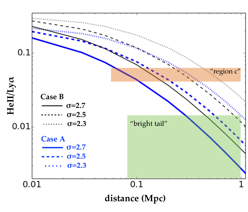
Figure 9: observed He ii/Ly$\alpha$ ratio obtained by our photoionisation model using a log-normal density distribution with $\langle n\rangle_{c}=0.05$ cm^-3 for both Case A and Case B effective and total recombination coefficients. The results are shown as a function of distance from the ionizing source for three values of the lognormal dispersion $\sigma$ (see legend for details). The shaded areas represent the allowed parameter space for both the “region c” and the “bright tail” regions as described in detail in the text.

References

- Arrigoni Battaia et al. (2015) Arrigoni Battaia F., Hennawi J. F., Prochaska J. X., Cantalupo S., 2015, ApJ, 809, 163
- Arrigoni Battaia et al. (2016) Arrigoni Battaia F., Hennawi J. F., Cantalupo S., Prochaska J. X., 2016, ApJ, 829, 3
- Arrigoni Battaia et al. (2018) Arrigoni Battaia F., Prochaska J. X., Hennawi J. F., Obreja A., Buck T., Cantalupo S., Dutton A. A., Macciò A. V., 2018, MNRAS, 473, 3907
- Bacon et al. (2015) Bacon R., et al., 2015, A&A, 575, A75
- Bacon et al. (2017) Bacon R., et al., 2017, A&A, 608, A1
- Bennett et al. (2014) Bennett C. L., Larson D., Weiland J. L., Hinshaw G., 2014, ApJ, 794, 135
- Bertin & Arnouts (1996) Bertin E., Arnouts S., 1996, A&AS, 117, 393
- Binette et al. (1996) Binette L., Wilson A. S., Storchi-Bergmann T., 1996, A&A, 312, 365
- Bond et al. (1996) Bond J. R., Kofman L., Pogosyan D., 1996, Nature, 380, 603
- Borisova et al. (2016) Borisova E., et al., 2016, ApJ, 831, 39
- Bouwens et al. (2014) Bouwens R. J., et al., 2014, ApJ, 793, 115
- Cai et al. (2017) Cai Z., et al., 2017, ApJ, 837, 71
- Cai et al. (2018) Cai Z., et al., 2018, ApJ, 861, L3
- Cantalupo (2017) Cantalupo S., 2017, in Fox A., Davé R., eds, Astrophysics and Space Science Library Vol. 430, Gas Accretion onto Galaxies. p. 195 (arXiv:1612.00491), doi:10.1007/978-3-319-52512-9˙9
- Cantalupo & Porciani (2011) Cantalupo S., Porciani C., 2011, MNRAS, 411, 1678
- Cantalupo et al. (2005) Cantalupo S., Porciani C., Lilly S. J., Miniati F., 2005, ApJ, 628, 61
- Cantalupo et al. (2007) Cantalupo S., Lilly S. J., Porciani C., 2007, ApJ, 657, 135
- Cantalupo et al. (2008) Cantalupo S., Porciani C., Lilly S. J., 2008, ApJ, 672, 48
- Cantalupo et al. (2012) Cantalupo S., Lilly S. J., Haehnelt M. G., 2012, MNRAS, 425, 1992
- Cantalupo et al. (2014) Cantalupo S., Arrigoni-Battaia F., Prochaska J. X., Hennawi J. F., Madau P., 2014, Nature, 506, 63
- Childs et al. (2012) Childs H., et al., 2012, in , High Performance Visualization–Enabling Extreme-Scale Scientific Insight. pp 357–372
- Dong et al. (2005) Dong X.-B., Zhou H.-Y., Wang T.-G., Wang J.-X., Li C., Zhou Y.-Y., 2005, ApJ, 620, 629
- Elmegreen (2002) Elmegreen B. G., 2002, ApJ, 577, 206
- Elvis (2000) Elvis M., 2000, ApJ, 545, 63
- Emonts et al. (2018) Emonts B. H. C., et al., 2018, MNRAS, 477, L60
- Farina et al. (2017) Farina E. P., et al., 2017, ApJ, 848, 78
- Fumagalli et al. (2016) Fumagalli M., Cantalupo S., Dekel A., Morris S. L., O’Meara J. M., Prochaska J. X., Theuns T., 2016, MNRAS, 462, 1978
- Fumagalli et al. (2017a) Fumagalli M., Haardt F., Theuns T., Morris S. L., Cantalupo S., Madau P., Fossati M., 2017a, MNRAS, 467, 4802
- Fumagalli et al. (2017b) Fumagalli M., et al., 2017b, MNRAS, 471, 3686
- Gallego et al. (2018) Gallego S. G., et al., 2018, MNRAS, 475, 3854
- Gaskell & Harrington (2018) Gaskell C. M., Harrington P. Z., 2018, MNRAS, 478, 1660
- Ginolfi et al. (2018) Ginolfi M., Maiolino R., Carniani S., Arrigoni Battaia F., Cantalupo S., Schneider R., 2018, MNRAS, 476, 2421
- Gould & Weinberg (1996) Gould A., Weinberg D. H., 1996, ApJ, 468, 462
- Hatch et al. (2008) Hatch N. A., Overzier R. A., Röttgering H. J. A., Kurk J. D., Miley G. K., 2008, MNRAS, 383, 931
- Heckman et al. (1991) Heckman T. M., Lehnert M. D., Miley G. K., van Breugel W., 1991, ApJ, 381, 373
- Hennawi et al. (2015) Hennawi J. F., Prochaska J. X., Cantalupo S., Arrigoni-Battaia F., 2015, Science, 348, 779
- Hogan & Weymann (1987) Hogan C. J., Weymann R. J., 1987, MNRAS, 225, 1P
- Humphrey et al. (2008) Humphrey A., Villar-Martín M., Vernet J., Fosbury R., di Serego Alighieri S., Binette L., 2008, MNRAS, 383, 11
- Humphrey et al. (2018) Humphrey A., Villar-Martín M., Binette L., Raj R., 2018, arXiv e-prints,
- Husemann et al. (2013) Husemann B., Wisotzki L., Sánchez S. F., Jahnke K., 2013, A&A, 549, A43
- Ji et al. (2018) Ji S., Oh S. P., McCourt M., 2018, MNRAS, 476, 852
- Kollmeier et al. (2010) Kollmeier J. A., Zheng Z., Davé R., Gould A., Katz N., Miralda-Escudé J., Weinberg D. H., 2010, ApJ, 708, 1048
- Lee et al. (2018) Lee K.-G., et al., 2018, ApJS, 237, 31
- Leibler et al. (2018) Leibler C. N., Cantalupo S., Holden B. P., Madau P., 2018, MNRAS, 480, 2094
- Lusso et al. (2015) Lusso E., Worseck G., Hennawi J. F., Prochaska J. X., Vignali C., Stern J., O’Meara J. M., 2015, MNRAS, 449, 4204
- Mandelker et al. (2016) Mandelker N., Padnos D., Dekel A., Birnboim Y., Burkert A., Krumholz M. R., Steinberg E., 2016, MNRAS, 463, 3921
- Marino et al. (2018) Marino R. A., et al., 2018, ApJ, 859, 53
- Martin et al. (2014) Martin D. C., Chang D., Matuszewski M., Morrissey P., Rahman S., Moore A., Steidel C. C., 2014, ApJ, 786, 106
- Martin et al. (2015) Martin D. C., Matuszewski M., Morrissey P., Neill J. D., Moore A., Cantalupo S., Prochaska J. X., Chang D., 2015, Nature, 524, 192
- Meiksin (2009) Meiksin A. A., 2009, Reviews of Modern Physics, 81, 1405
- Miley & De Breuck (2008) Miley G., De Breuck C., 2008, A&ARv, 15, 67
- Morais et al. (2017) Morais S. G., et al., 2017, MNRAS, 465, 2698
- Myers (1978) Myers P. C., 1978, ApJ, 225, 380
- North et al. (2017) North P. L., et al., 2017, A&A, 604, A23
- Osterbrock (1989) Osterbrock D. E., 1989, Astrophysics of gaseous nebulae and active galactic nuclei
- Otí-Floranes & Mas-Hesse (2010) Otí-Floranes H., Mas-Hesse J. M., 2010, A&A, 511, A61
- Padnos et al. (2018) Padnos D., Mandelker N., Birnboim Y., Dekel A., Krumholz M. R., Steinberg E., 2018, MNRAS, 477, 3293
- Padoan & Nordlund (2002) Padoan P., Nordlund Å., 2002, ApJ, 576, 870
- Peterson et al. (2004) Peterson B. M., et al., 2004, ApJ, 613, 682
- Prescott et al. (2015) Prescott M. K. M., Martin C. L., Dey A., 2015, ApJ, 799, 62
- Rauch (1998) Rauch M., 1998, ARA&A, 36, 267
- Rauch et al. (2008) Rauch M., et al., 2008, ApJ, 681, 856
- Ross et al. (2018) Ross N. P., et al., 2018, MNRAS, 480, 4468
- Silva et al. (2018) Silva M., et al., 2018, MNRAS, 474, 3649
- Soto et al. (2016) Soto K. T., Lilly S. J., Bacon R., Richard J., Conseil S., 2016, MNRAS, 458, 3210
- Vanden Berk et al. (2004) Vanden Berk D. E., et al., 2004, ApJ, 601, 692
- Villar-Martín (2007) Villar-Martín M., 2007, New Astron. Rev., 51, 194
- Villar-Martín et al. (2007) Villar-Martín M., Humphrey A., De Breuck C., Fosbury R., Binette L., Vernet J., 2007, MNRAS, 375, 1299
- Wada & Norman (2007) Wada K., Norman C. A., 2007, ApJ, 660, 276
- Weilbacher et al. (2016) Weilbacher P. M., Streicher O., Palsa R., 2016, MUSE-DRP: MUSE Data Reduction Pipeline, Astrophysics Source Code Library (ascl:1610.004)
- Wright (2006) Wright E. L., 2006, PASP, 118, 1711