Spectrum of the open QCD flux tube and its effective string description

Abstract:

I perform a high precision measurement of the static quark-antiquark potential in three-dimensional ${\rm SU}(N)$ gauge theory with $N=2$ to 6. The results are compared to the effective string theory for the QCD flux tube and I obtain continuum limit results for the string tension and the non-universal leading order boundary coefficient, including an extensive analysis of all types of systematic uncertainties. The magnitude of the boundary coefficient decreases with increasing $N$, but remains non-vanishing in the large-$N$ limit. I also test for the presence of possible contributions from rigidity or massive modes and compare the results for the string theory parameters to data for the excited states.

1 Introduction

The observation that the lowest lying mesons can be grouped in so-called Regge-trajectories has lead to the formulation of the first string theories [1, 2] to describe the strong interactions. This string picture even persists until today, after the introduction of Quantum Chromodynamics (QCD) as the fundamental theory for the strong interactions, in terms of an effective string theory (EST) for mesons and baryons. The basic idea is that, for large quark distances, the chromo-electromagnetic field connecting the quarks is squeezed into a narrow, tube-alike region, a flux tube, via a dual version of the Meissner effect. For a quark-antiquark ($q\bar{q}$) pair, i.e., a mesonic state, this is shown

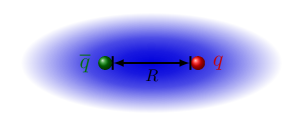
$\Big{\Downarrow}$ enlarging $R$

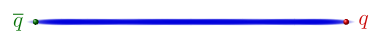
Figure 1: Schematic picture of flux tube formation for a static $q\bar{q}$ pair.

schematically in Fig. 1. As soon as the width of the flux tube becomes negligible compared to the $q\bar{q}$ separation $R$, the flux tube effectively looks like a thin energy string (also denoted as the confining string in this framework) and its dynamics is governed by stringy excitations described by the EST. The resulting dominant term in the energy levels at large $R$ is a linear term of the form $\sigma R$, where $\sigma$ is the energy per unit length of the flux tube, known as the string tension. Consequently, flux tube formation provides a heuristic mechanism to explain quark confinement in QCD (see Ref. [3] for a review). In QCD with finite quark masses, the flux tube persists only up to $q\bar{q}$ distances where the potential energy in the system allows to create another $q\bar{q}$ pair from the vacuum, leading to a state with two instead of one mesons. This effect is known as string breaking (see Ref. [4] for a study in full QCD, for instance) and it is the reason why quarks have not been observed as free particles in nature.

In the static limit, the energy of a $q\bar{q}$ pair at distance $R$ is related to the static quark-antiquark potential $V(R)$. Similar potentials can also be defined for mesonic states with excited gluon configurations carrying non-trivial quantum numbers. These potentials are, besides their relevance concerning the anatomy of confinement, important for the theoretical description of heavy quarkonia and hybrid mesons. To study these systems the availability of an analytic expression for the potentials is important and the EST can provide valuable input.

Figure 2: Schematic picture of the projection of the 10-dimensional string in a generalization of the AdS/CFT correspondence to large-$N$ gauge theories onto the 4-dimensional boundary of the AdS space. The boundary is associated with the spacetime of pure gauge theory.

Apart from these phenomenological applications, the EST provides a natural framework to make contact with a possible 10-dimensional (10d) string theory dual to large-$N$ gauge theories in terms of a generalization of the AdS/CFT correspondence [8]. In principle, the EST action can be computed from the 10d string theory by integrating out the additional massive modes (see Ref. [9] and references therein). In terms of this correspondence the confining string can be visualized, as shown in Fig. 2, as the 4d projection of the 10d string onto the boundary of the anti-de Sitter space, associated with the spacetime of the gauge theory. When computed from the fundamental string theory, possible non-universal parameters in the EST action are related to properties of the AdS side of the duality. A particular example is the boundary coefficient $\bar{b}_{2}$, introduced in the next section, which, for certain holographic string backgrounds, can be related to the masses of the additional bosonic and fermionic degrees of freedom of the fundamental string theory [10]. Knowledge about the non-universal parameters in the $N\to\infty$ limit can thus be converted into constraints for the 10d string theory in AdS spacetime and help to find suitable backgrounds for the gauge/gravity correspondence of non-conformal gauge theories. See Refs. [11, 12, 13] for recent computations of properties of flux tubes in this framework.

The energy levels of the flux tube and the associated potentials can be computed in pure gauge theory on the lattice. A recent collection of results can be found in Ref. [14]. All of the results so far have shown remarkable agreement with the predictions from the EST down to comparably small values of $\sqrt{\sigma}R\approx 1.2-1.5$. Note, that the EST, as an effective theory for long flux tubes, is expected to break down at around $\sqrt{\sigma}R\lesssim 1$. In 4d, energy states of closed flux tubes have been found recently [15] which are consistently described by massive modes on the string worldsheet [16, 17]. Open string states with a similar behavior have also been observed earlier [18]. The appearance of such states is certainly expected, given the differences between the flux tube and a string. The finite width of the flux tube may allow for inner vibrations and torsions, which could show up as massive modes in the spectrum. A peculiar feature is the apparent absence of massive modes in the 3d data. A theoretical explanation for this is the fact that the coupling term between the massive mode and the Goldstone bosons does not exist in 3d. From the phenomenological point of view, neither torsions nor the development of knots are possible, since there is only one transverse direction. Thus the absence of the massive modes in 3d is plausible if the low lying massive modes are related to either of these phenomena. In 3d we are left with vibration modes and contributions due to the string rigidity. The latter has been first proposed by Polyakov [19] and recently found to be essential to describe the potential in 3d ${\rm U}(1)$ gauge theory [20]. Rigidity contributions appear at high orders in the $1/R$ expansion, but the presence of the rigidity term gives a non-perturbative contribution to the potential [21, 22, 20]. Formally its contribution is similar to the one of a free massive mode on the worldsheet (coupling to the Goldstone bosons only via the induced metric).

In this proceedings article I report on the progress concerning my studies [23, 24, 25, 26] of the energy levels of the flux tube and their comparison to the EST in 3d ${\rm SU}(N)$ gauge theories for $N\to\infty$. I will show continuum extrapolated results for the string tension (comparing also to the Karabali-Kim-Nair (KKN) prediction [27]) and the boundary coefficient $\bar{b}_{2}$ for $N=2$ to 6, which are then extrapolated to the large-$N$ limit. $\bar{b}_{2}$ is first obtained from an analysis excluding massive modes or contributions from rigidity. In the second step we test whether such modes can be present, how they change the value of $\bar{b}_{2}$ and extract their mass.

2 EST predictions and massive/rigid modes

The EST describes the dynamics of a stable non-interacting flux tube in terms of the quantized transverse oscillation modes, the Goldstone bosons associated with the breaking of the translational symmetry by the tube. The basic properties of the theory are known for some time [28, 29, 30] but a number of features have only been elucidated recently (for reviews see [31, 14]). The spectrum has been computed up to $O(R^{-5})$ [32, 33],

$$\begin{array}[]{rl}\displaystyle E^{\rm EST}_{n,l}(R)&\displaystyle=\sigma\>R\>\sqrt{1+\frac{2\pi}{\sigma\>R^{2}}\>\left(n-\frac{1}{24}\>(d-2)\right)}\vspace*{2mm}\\ &\displaystyle-\bar{b}_{2}\frac{\pi^{3}}{\sqrt{\sigma^{3}}R^{4}}\Big{(}B_{n}^{l}+\frac{d-2}{60}\Big{)}-\frac{\pi^{3}(d-26)}{48\sigma^{2}R^{5}}C_{n}^{l}+O(R^{-\xi})\,.\end{array}$$ (1)

The leading order term, the first term on the right-hand-side, is the spectrum obtained from the light cone quantization [34] of the Nambu-Goto string (LC spectrum). $B_{n}^{l}$ and $C_{n}^{l}$ are dimensionless coefficients, depending on the representation of the state with respect to rotations around the string axis (see [26]). The term proportional to $\bar{b}_{2}$ is the leading order boundary correction (BC). For the groundstate in 3d $B_{0}^{0}$ and $C_{0}^{0}$ vanish, so that the BC is the only correction term up to $O(R^{-6})$. $\bar{b}_{2}$ has previously been computed in 3d ${\rm SU}(2)$ [24] and $Z(2)$ gauge theories [35].

In the energy levels of Eq. (1), possible contributions from rigidity or massive modes have not been included. In 3d contributions from rigidity and massive bosons on the worldsheet are formally equivalent. In $\zeta$-function regularization and including higher order terms perturbatively, the rigidity/massive mode corrections are given by [20]

$$V^{\rm rig}(R)=-\frac{m}{2\pi}\sum_{k=1}^{\infty}\frac{K_{1}(2kmR)}{k}-\frac{(d-2)(d-10)\pi^{2}}{3840m\sigma R^{4}}\,.$$ (2)

Here $m$ is the mass parameter, which is related to the rigidity parameter in case of a correction originating from the string rigidity, and $K_{1}$ is a modified Bessel functions of the second kind. The second term on the right-hand-side contaminates the BC term and thus changes the value of $\bar{b}_{2}$. Note, that the $\zeta$-function regularization scheme breaks Lorentz symmetry, so that counterterms may need to be taken into account for a proper extraction of the energy levels [36]. From now on we will always refer to the correction terms from Eq. (2) as “massive mode” contributions.

3 String tension and KKN prediction

We perform simulations in 3d ${\rm SU}(N)$ ($N=2$ to 6) gauge theory using the standard mixture of heatbath and overrelaxation steps. The potential is extracted from Polyakov loop correlation functions, which are computed with one level of the Lüscher-Weisz multilevel algorithm [37] for error reduction. We used 20000 sublattice updates and temporal sublattice sizes ranging between 2 and 12. For more details and a study of systematic effects see Ref. [26]. For scale setting we use the Sommer scale $r_{0}=0.5$ fm [38], which may be used to translate to “physical” units. For each value of $N$ we have simulated at least 3 lattice spacings, keeping the spatial and temporal extents larger than $10\,r_{0}$ to render finite size effects negligible. The potential has been extracted up to $R/r_{0}\gtrsim 3$ for all lattice spacings.

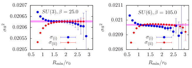
Figure 3: Results for the string tension extracted from fits (i), $\sigma_{\rm(i)}$, and (ii), $\sigma_{\rm(ii)}$, as explained in the text, versus $R_{\rm min}$ in units of $r_{0}$ for $N=3$ (left) and 6 (right). The magenta bands are the values for $\sigma_{(ii)}$ used in the further analysis.

We start by extracting the string tension $\sigma$ in a way that we can control the effect of higher order corrections. To this end we use of two different fits: (i) we fit the force ($F(R)=\partial V/[\partial R]$) to the form $\>R^{2}F(R)=\sigma R^{2}+\gamma$; (ii) we fit $V(R)$ to the LC potential, adding a normalization constant $V_{0}$. The fits include different terms of the $1/R$ expansion starting at $O(1/R^{3})$, so that the results will differ once corrections at this order become important. To isolate the asymptotic behavior, one can thus investigate the dependence of the fit parameters on the minimal value of $R$ included in the fit, $R_{\rm min}$. In the region where the results from the fits agree within errors and show a plateau the estimate for $\sigma$ from either of the methods will be reliable within the given uncertainties. Two typical examples for the $R_{\rm min}$ dependence of $\sigma$ obtained from the two fits, denoted as $\sigma_{\rm(i)}$ and $\sigma_{\rm(ii)}$, respectively, are shown in Fig. 3. In the following we will always use the result $\sigma_{\rm(ii)}$ obtained with the value of $R_{\rm min}$ where the results of the two methods become fully consistent (indicated by the magenta bands in Fig. 3). We extrapolate $\sqrt{\sigma}r_{0}$ to the continuum including terms of $O(a^{2})$ and $O(a^{4})$. The systematic uncertainty of this extrapolation is estimated by comparison to a fit for the data with $r_{0}/a\gtrsim 6$, including only a term of $O(a^{2})$. The continuum results for $\sigma$ are shown in Fig. 4 (left) versus $1/N^{2}$.

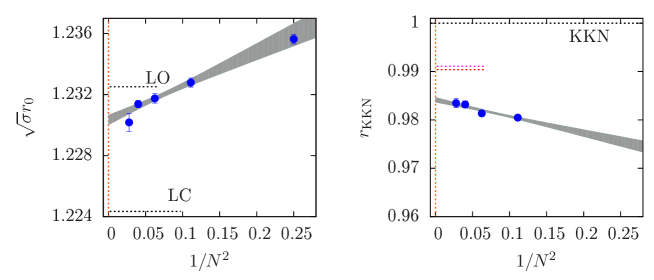
Figure 4: Continuum results for $\sqrt{\sigma}$ (left) and the ratio $r_{\rm KKN}$ (right) versus $1/N^{2}$. The curves are the large-$N$ extrapolations. The dashed line in the left plot labeled by ‘LC’ indicates the values of $\sqrt{\sigma}r_{0}$ obtained from the full LC spectrum and the one labeled by ‘LO’ is the result from the expansion to $O(1/R)$. The dashed lines in the right plot are the results for $r_{\rm KKN}$ from [40] (red) and [41] (magenta).

To compare to the KKN prediction [27],

$$\frac{\sqrt{\sigma}}{g_{\rm MF}^{2}}=\sqrt{\frac{N^{2}-1}{8\pi}}\,,\quad\textnormal{with}\quad g_{\rm MF}^{2}=\frac{2N}{\beta\big{<}U_{p}\big{>}}\,,$$ (3)

the mean-field improved coupling [39], and the plaquette expectation value $\big{<}U_{p}\big{>}$, we define

$$r_{\rm KKN}=\frac{\big{(}\sqrt{\sigma}/g_{\rm MF}^{2}\big{)}_{\rm lat}}{\sqrt{(N^{2}-1)/(8\pi)}}\,,$$ (4)

where the denominator includes the lattice result. We compute the ratio in the continuum using a continuum extrapolation of $g_{\rm MF}^{2}$ in units of $r_{0}$ as for $\sigma$ with $a^{2}\to a$. The results for the ratio are shown in Fig. 4 (right).

Finally, we extrapolate the results to $N\to\infty$ using a function linear in $1/N^{2}$ excluding the data with $N=2$. The resulting extrapolations are shown by the gray curves in both panels of Fig. 4. To quantify the systematic uncertainty of the extrapolation, we repeat the extrapolation excluding the $N=3$ result. The results for $\sigma$ and $r_{\rm KKN}$ in the large-$N$ limit are

$$r_{0}\sqrt{\sigma}^{N\to\infty}=1.2304(5)\quad\textnormal{and}\quad r_{\rm KKN}^{N\to\infty}=0.9842(15)\,.$$ (5)

The value for $\sqrt{\sigma}r_{0}$ is unambiguously determined within the EST and we display the values for the LC spectrum and its leading order (LO) expansion in $1/R$ by the dashed lines in Fig. 4. The large-$N$ extrapolation clearly lies between the two cases, indicating that corrections to the LC spectrum are mandatory to describe the large-$N$ potential down to $R=r_{0}$. In the right panel of Fig. 4 we also show results for $r_{\rm KKN}$ from the literature [40, 41] (dashed lines). Our results turn out to be somewhat smaller than the ones from previous computations.

4 EST analysis without massive modes

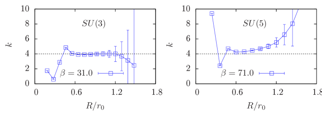
Figure 5: Examples for the dependence of the exponent $k$ on $R_{\rm min}$ for $N=3$ (left) and 5 (right).

The EST predicts corrections to the LC spectrum starting at $O(R^{-4})$. To test whether this is reflected by the data we fit them to the form

$$V(R)=\sigma\>R\>\sqrt{1-\frac{\pi}{12\>\sigma\>R^{2}}}+\frac{\eta}{\big{(}\sqrt{\sigma}R\big{)}^{k}}+V_{0}\,,$$ (6)

where $k$, $\eta$, $\sigma$ and $V_{0}$, are fit parameters. If the data agree with the EST predictions, we expect to see a clear plateau at $k=4$ when $k$ is plotted versus $R_{\rm min}$. Two typical examples for the $R_{\rm min}$ dependence of $k$ are shown in Fig. 5. While the results for ${\rm SU}(3)$ indicate a clear plateau at $k=4$, the ${\rm SU}(5)$ results show values of $k\gtrsim 4$. This is generally the case for larger $N$ and possibly indicates a decrease of $\bar{b}_{2}$ (which we will indeed find below), so that higher order corrections become more important with increasing $N$.

To extract $\bar{b}_{2}$, at this point neglecting massive mode corrections, we use the general fit formula

$$V(R)=E^{\rm EST}_{0}(R)+\frac{\gamma^{(1)}_{0}}{\sqrt{\sigma^{5}}R^{6}}+\frac{\gamma^{(2)}_{0}}{\sigma^{3}R^{7}}+V_{0}\,.$$ (7)

Here $E^{\rm EST}_{0}$ is the energy level with $N,l=0$ from Eq. (1) and $\gamma^{(1)}_{0}$, $\gamma^{(2)}_{0}$ and $V_{0}$ are fit parameters along with $\sigma$ and $\bar{b}_{2}$. We perform five different fits:

1. take $\sigma$ and $V_{0}$ from Sec. 3, use $\bar{b}_{2}$, $\gamma^{(1)}_{0}$ and $\gamma^{(2)}_{0}$ as free parameters;

2. use $\sigma$, $V_{0}$ and $\bar{b}_{2}$ as free parameters, set $\gamma^{(1)}_{0}=0$ and $\gamma^{(2)}_{0}=0$;

3. use $\sigma$, $V_{0}$, $\bar{b}_{2}$ and $\gamma^{(1)}_{0}$ as free parameters, set $\gamma^{(2)}_{0}=0$;

4. use $\sigma$, $V_{0}$, $\bar{b}_{2}$ and $\gamma^{(2)}_{0}$ as free parameters, set $\gamma^{(1)}_{0}=0$;

5. use $\sigma$, $V_{0}$, $\gamma^{(1)}_{0}$ and $\gamma^{(2)}_{0}$ as free parameters, set $\bar{b}_{2}=0$.

For all of the fits we use the second smallest value for $R_{\rm min}$ for which $\chi^{2}/$dof$<1.5$. Better or worse agreement with the data is then indicated by the value of $R_{\rm min}$ in combination with the number of higher order terms included in the fit. For fit C, for instance, we expect a smaller value of $R_{\rm min}$ compared to fit B, which does not contain higher order corrections. For all parameter sets fit E demands larger values for $R_{\rm min}$ compared to fits C and D, indicating less agreement with the data. This is possibly due to the fact that both correction terms are needed to mimic the $1/R^{4}$ term at intermediate distances, which shows that the $1/R^{4}$ term is necessary to successfully describe the data. For fit A, $R_{\rm min}$ has to be larger than for fits C and D, showing that it is too restrictive to fix the values of $\sigma$ and $V_{0}$ in the fits, even though the change of $\sigma$ is not significant. In the following we thus use fits B to D and their weighted average as the final result.

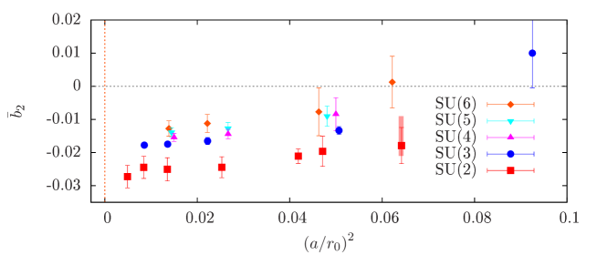
Figure 6: Results for the boundary coefficient $\bar{b}_{2}$ for the individual lattices versus the squared lattice spacing in units of $r_{0}$. The red band indicates the result for $\bar{b}_{2}$ obtained from the excited states in [24].

The results for $\bar{b}_{2}$ are shown in Fig. 6. The uncertainties also include the systematic uncertainty associated with the particular choice for $R_{\rm min}$, estimated from the fit results obtained with $R_{\rm min}\to R_{\rm min}\pm 1a$, and from the unknown higher order terms, estimated by the spread of the results from fits B to D. For the continuum extrapolation we employ a function linear in $a^{2}$. To estimate the systematics associated with this choice, we compare the result to the ones obtained including only the data with $(a/r_{0})>0.2$. For error propagation of the other systematic uncertainties, we perform all possible combinations of continuum (and later also large-$N$) extrapolations and compute the individual systematic uncertainties as described above. The continuum results for $\bar{b}_{2}$ are plotted in Fig. 7.

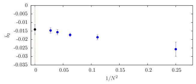
Figure 7: Continuum results for the boundary coefficient $\bar{b}_{2}$ versus $1/N^{2}$. The black point is the result in the large-$N$ limit.

We extrapolate $\bar{b}_{2}$ to the large-$N$ limit using a linear function in $1/N^{2}$ including data with $N>2$. As for the continuum extrapolation, we estimate the systematic uncertainty by comparison to an extrapolation including data with $N>3$. We obtain

$$\bar{b}^{N\to\infty}_{2}=-0.0141(3)(15)(13)(9)(17)\,.$$ (8)

The first uncertainty is purely statistical, the second is the systematic one associated with the higher order corrections, the third is the one for the choice of $R_{\rm min}$, the fourth is the one of the continuum extrapolation and the fifth the one of the large-$N$ extrapolation. The final result is also shown as the black point in Fig. 7.

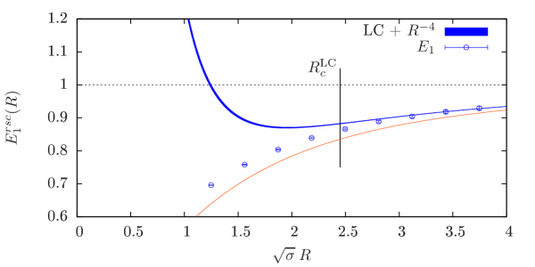
Figure 8: Comparison between the EST prediction and the data for the first excited state $E_{1}$ for ${\rm SU}(2)$ at $\beta=5.0$. The red curve is the difference from the LC spectrum and the one labeled with ‘LC$+R^{-4}$’ includes the BC term. The vertical line with label ‘$R_{c}^{\rm LC}$’ indicates the radius of convergence for the series expansion in $1/R$ of the first excited state of the LC spectrum.

Finally, we test the consistency with the excited states. In the EST the energies are fully determined by $\sigma$, $V_{0}$ and $\bar{b}_{2}$ up to higher order terms. We compare the EST prediction for the first excited state with the data for ${\rm SU}(2)$ at $\beta=5.0$ from Ref. [24] in Fig. 8. The data show good agreement with the curve up to $\sqrt{\sigma}R\approx 3$, where deviations due to higher order terms become visible. In fact, a naive fit including a term of $O(1/R^{6})$ agrees with the data down to $\sqrt{\sigma}R\approx 1.8$. One can also extract $\bar{b}_{2}$ from the excited states [24]. The result, which is in excellent agreement with the analysis of the potential, is shown as the red band in Fig. 8. We thus conclude that the results for $\bar{b}_{2}$ are fully consistent with the excited state data. A more detailed comparison is planned for the near future.

5 Testing the presence of massive modes

So far we have neglected possible massive-mode contributions. To test how they would affect the results for $\bar{b}_{2}$ we repeat the analysis from the previous section employing a fit function of the form

$$V(R)=E_{0}^{\rm EST}(R)-\frac{m}{2\pi}\sum_{k=1}^{\infty}\frac{K_{1}(2kmR)}{k}-\frac{(d-2)(d-10)\pi^{2}}{3840m\sigma R^{4}}+\frac{\gamma^{(1)}_{0}}{\sqrt{\sigma^{5}}R^{6}}+\frac{\gamma^{(2)}_{0}}{\sigma^{3}R^{7}}+V_{0}\,.$$ (9)

In practice, the infinite sum is completely dominated by the first few terms, so that it is sufficient to use the first 100 terms to reach machine precision. We perform four different fits:

1. use $\sigma$, $V_{0}$, $\bar{b}_{2}$ and $m$ as free parameters, set $\gamma^{(1)}_{0}=\gamma^{(2)}_{0}=0$;

2. use $\sigma$, $V_{0}$, $\bar{b}_{2}$, $m$ and $\gamma^{(1)}_{0}$ as free parameters, set $\gamma^{(2)}_{0}=0$;

3. use $\sigma$, $V_{0}$, $\bar{b}_{2}$, $m$ and $\gamma^{(2)}_{0}$ as free parameters, set $\gamma^{(1)}_{0}=0$;

4. use $\sigma$, $V_{0}$ and $m$ as free parameters, set $\gamma^{(1)}_{0}=\gamma^{(2)}_{0}=\bar{b}_{2}=0$.

The last fit is similar to fit E above and checks whether the $R^{-4}$ term from Eq. (2) is already sufficient to describe the data. As before, however, we find that fit J needs much larger values of $R_{\rm min}$ and, consequently, does not compare equally well to the data as the other fits. Unfortunately, the results from fits G and H are not sufficiently precise, since the fits contain two higher order terms. In the following we will thus only use fit F. Note, that this impedes the estimation of the systematic uncertainty due to possible higher order terms.

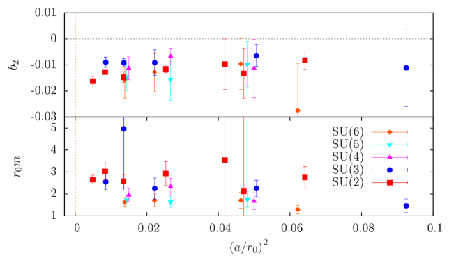
Figure 9: Results for the boundary coefficient $\bar{b}_{2}$ and the mass $m$ in units if $r_{0}$ for the individual lattices versus the squared lattice spacing.

We show the results for $\bar{b}_{2}$ and $m$ in figure 9. Due to the additional $R^{-4}$ term, the results for $\bar{b}_{2}$ move closer to zero and, in general, the uncertainties for $\bar{b}_{2}$ increase. The results for $m$ approach the continuum smoothly, enabling a linear continuum extrapolation. The continuum results are shown in Fig. 10. While the uncertainties for $\bar{b}_{2}$ are too large to perform a reliable extrapolation to $N\to\infty$, the results for $m$ allow for a reliable large-$N$ extrapolation and the final result is

$$r_{0}m^{N\to\infty}=1.34(4)(8)(25)(27)\,,\quad\textnormal{or}\quad\frac{m^{N\to\infty}}{\sqrt{\sigma}^{N\to\infty}}=1.1(4)\,.$$ (10)

Here the first uncertainty is purely statistical, the second is the systematic uncertainty associated with $R_{\rm min}$, the third is the one of the continuum extrapolation and the fourth is the one of the large-$N$ extrapolation. This result can be compared to the one for the massive mode in 4d, $m^{N\to\infty}/\sqrt{\sigma}^{N\to\infty}=1.713(4)$ [42]. While $m$ appears to be somewhat smaller in 3d, one has to keep in mind, that the 4d result is not continuum extrapolated. It is thus possible, that we are actually seeing a similar massive mode in 3 and 4 dimensions.

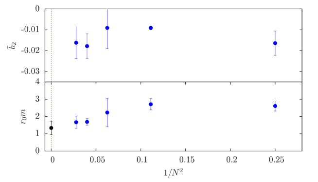
Figure 10: Continuum results for the boundary coefficient $\bar{b}_{2}$ and the mass $m$ versus $1/N^{2}$. The black point for $m$ is the result in the large-$N$ limit.

We can again compare the result for $\bar{b}_{2}$ with the ${\rm SU}(2)$, $\beta=5.0$ results for the excited states. The comparison is shown in Fig. 11. The prediction (blue curve) lies below the data even at large $R$. Naively, this implies a contradiction with the excited state data. However, the excited state contributions of the massive mode are unknown, rendering the comparison incomplete.

Figure 11: Comparison between the EST prediction and the data for $E_{1}$ for ${\rm SU}(2)$ and $\beta=5.0$ as in Fig. 8. The blue curve now includes $\bar{b}_{2}$ obtained from the analysis with massive modes, while the gray curve is the one from Fig. 8.

6 Conclusions

In this proceedings article I provided an update on my studies of the energy levels of the (open) flux tube and their comparison to the EST in 3d ${\rm SU}(N)$ gauge theories. I obtain continuum and large-$N$ extrapolated results for the EST parameters with full control over the relevant systematic effects. The large-$N$ extrapolated results are given in Eqs. (5), (8) and (10). I have also shown that the leading order correction to the LC spectrum is indeed of $O(R^{-4})$. The main uncertainty for $\bar{b}_{2}$ concerns the presence or absence of massive modes. In both cases, however, $\bar{b}_{2}$ remains non-vanishing at finite $N$ and, likely, also in the large-$N$ limit (cf. Fig. 10). It would be interesting to obtain a prediction for the contribution of massive modes to the excited states. This could potentially help to either rule out or confirm the presence of massive modes and might even enable the discrimination of massive mode and rigidity contributions. It is intriguing to see that the result for $m$ is in good agreement with the masses found in [42], providing a hint for a similar origin of the massive modes in 3d and 4d. In the large-$N$ limit the KKN prediction agrees with the lattice result up to 1.6%, which is about a factor of two further away than previous findings [40, 41].

References

- [1] T. Goto, Prog. Theor. Phys. 46 (1971) 1560.
- [2] P. Goddard, J. Goldstone, C. Rebbi and C. B. Thorn, Nucl. Phys. B 56 (1973) 109.
- [3] J. Greensite, Prog. Part. Nucl. Phys. 51 (2003) 1 [hep-lat/0301023].
- [4] G. S. Bali et al. [SESAM Collaboration], Phys. Rev. D 71 (2005) 114513 [hep-lat/0505012].
- [5] N. Brambilla et al., Eur. Phys. J. C 71 (2011) 1534 [arXiv:1010.5827].
- [6] C. A. Meyer and E. S. Swanson, Prog. Part. Nucl. Phys. 82 (2015) 21 [arXiv:1502.07276].
- [7] S. Capitani et al, arXiv:1811.11046.
- [8] J. M. Maldacena, Int. J. Theor. Phys. 38 (1999) 1113 [hep-th/9711200].
- [9] O. Aharony and E. Karzbrun, JHEP 0906 (2009) 012 [arXiv:0903.1927].
- [10] O. Aharony and M. Field, JHEP 1101 (2011) 065 [arXiv:1008.2636].
- [11] U. Kol and J. Sonnenschein, JHEP 1105 (2011) 111 [arXiv:1012.5974].
- [12] V. Vyas, Phys. Rev. D 87 (2013) no.4, 045026 [arXiv:1209.0883].
- [13] D. Giataganas and N. Irges, JHEP 1505 (2015) 105 [arXiv:1502.05083].
- [14] B. B. Brandt and M. Meineri, Int. J. Mod. Phys. A 31 (2016) no.22, 1643001 [arXiv:1603.06969].
- [15] A. Athenodorou, B. Bringoltz and M. Teper, JHEP 1102 (2011) 030 [arXiv:1007.4720].
- [16] S. Dubovsky et al, Phys. Rev. Lett. 111 (2013) no.6, 062006 [arXiv:1301.2325].
- [17] S. Dubovsky, R. Flauger and V. Gorbenko, J. Exp. Theor. Phys. 120 (2015) 399 [arXiv:1404.0037].
- [18] K. J. Juge, J. Kuti and C. Morningstar, Phys. Rev. Lett. 90 (2003) 161601 [hep-lat/0207004].
- [19] A. M. Polyakov, Nucl. Phys. B 268 (1986) 406.
- [20] M. Caselle, M. Panero, R. Pellegrini and D. Vadacchino, JHEP 1501 (2015) 105 [arXiv:1406.5127].
- [21] T. R. Klassen and E. Melzer, Nucl. Phys. B 350 (1991) 635.
- [22] V. V. Nesterenko and I. G. Pirozhenko, J. Math. Phys. 38 (1997) 6265 [hep-th/9703097].
- [23] B. B. Brandt and P. Majumdar, Phys. Lett. B 682 (2009) 253 [arXiv:0905.4195].
- [24] B. B. Brandt, JHEP 1102 (2011) 040 [arXiv:1010.3625].
- [25] B. B. Brandt, PoS EPS -HEP2013 (2013) 540 [arXiv:1308.4993].
- [26] B. B. Brandt, JHEP 1707 (2017) 008 [arXiv:1705.03828].
- [27] D. Karabali, C. j. Kim and V. P. Nair, Phys. Lett. B 434 (1998) 103 [hep-th/9804132].
- [28] Y. Nambu, Phys. Lett. 80B (1979) 372.
- [29] M. Lüscher, K. Symanzik and P. Weisz, Nucl. Phys. B 173 (1980) 365.
- [30] A. M. Polyakov, Nucl. Phys. B 164 (1980) 171.
- [31] O. Aharony and Z. Komargodski, JHEP 1305 (2013) 118 [arXiv:1302.6257].
- [32] O. Aharony and N. Klinghoffer, JHEP 1012 (2010) 058 [arXiv:1008.2648].
- [33] O. Aharony, M. Field and N. Klinghoffer, JHEP 1204 (2012) 048 [arXiv:1111.5757].
- [34] J. F. Arvis, Phys. Lett. 127B (1983) 106.
- [35] M. Billo et al, JHEP 1205 (2012) 130 [arXiv:1202.1984].
- [36] S. Dubovsky, R. Flauger and V. Gorbenko, JHEP 1209 (2012) 044 [arXiv:1203.1054].
- [37] M. Lüscher and P. Weisz, JHEP 0109 (2001) 010 [hep-lat/0108014].
- [38] R. Sommer, Nucl. Phys. B 411 (1994) 839 [hep-lat/9310022].
- [39] G. P. Lepage and P. B. Mackenzie, Phys. Rev. D 48 (1993) 2250 [hep-lat/9209022].
- [40] B. Lucini and M. Teper, Phys. Rev. D 66 (2002) 097502 [hep-lat/0206027].
- [41] B. Bringoltz and M. Teper, PoS LAT 2006 (2006) 041 [hep-lat/0610035].
- [42] A. Athenodorou and M. Teper, Phys. Lett. B 771 (2017) 408 [arXiv:1702.03717].