Statistics-tuned phases of pseudofermions in one dimension

Abstract

We show that a quadratic system of pseudofermions, with tunable fractionalised statistics, can host a rich phase diagram on a one dimensional chain with nearest and next nearest neighbour hopping. Using a combination of numerical and analytical techniques, we show that that by varying the statistical angle and the ratio of the hopping, the system stabilizes two Tomonaga-Luttinger liquids (TLL) with central charges $c=1$ and $2$ respectively along with the inversion symmetry broken bond ordered (BO) insulating phase. Interestingly, the two quantum phase transitions in the system – (1) between the two TLLs, and, (2) the $c=1$ TLL and BO phase can be engendered by solely tuning the statistics of the pseudofermions. Our analysis shows that both these transition are continuous and novel with the former lacking a local order-parameter based description and the latter of Berezinskii-Kosterlitz-Thouless type. These phases and phase transitions can be of direct experimental relevance in context of recent studies of fermionic cold atoms.

Introduction :

Advances in the physics of one dimensional systems motivated by, inter alia, the possibility of Majorana zero modesKitaev_PU_2001; Alicea_RPP_2012; mourik2012signatures, have ushered in many new possibilities and opportunities. Particularly remarkable is the prospect of creating quantum entangled phases with fractional quantum numbers and statistics Leinaas_NC_1977; Lieb_PR_1963; Kundu_PRL_1999; Pasquier_IMS_1994; Ha_PRL_1994; Ha_NPB_1995. Several recent proposals indeed suggest that starting with bosons or fermions, effective local Hamiltonians with degrees of freedom following fractionalized or intermediate statistics can be realized, for example, in ultra-cold atomic systems Keilmann_NatCom_2011; Strater_PRL_2016; Greschner_PRL_2015; Cardarelli_PRA_2016; Greschner_PRA_2018. Exploring the physics of such system with tunable statistics has hence emerged as an active field of research.

In a one dimensional(D) chain with sites labeled $i,j$ etc., such tunable statistics is captured by the algebra generated by the onsite creation/annihilation operators given by

$$a_{j}a_{i}\pm a_{i}a_{j}e^{\mathbbm{i}\phi~{}sign(i-j)}= 0$$ (1)

$$a_{j}a^{\dagger}_{i}\pm a^{\dagger}_{i}a_{j}e^{-\mathbbm{i}\phi~{}sign(i-j)}= \delta_{ij}$$

$$[N_{i},a_{j}]=-\delta_{ij}a_{j};~{}~{}~{}[N_{i},a^{\dagger}_{j}] =\delta_{ij}a_{j}^{\dagger}$$

(where $N_{i}=a_{i}^{\dagger}a_{i}$). The underlying physics consistent with $sign(0)=0$ produces an onsite algebra that is bosonic or fermionic depending on the relative sign ($\pm$). Owing to this, we refer the two cases as pseudofermions ($+$ sign) or pseudobosons ($-$ sign) respectively even for $\phi\neq 0$. In either case, the off-site algebra can be tuned from fermionic to bosonic by tuning statistical parameter $\phi\in[0,\pi]$. Both pseudobosons and pseudofermions defined above are generalizations of two dimensional “anyons” to one spatial dimensions following Leinass and MyrheimLeinaas_NC_1977.

Subsequent works on exactly solvable one dimensional interacting bosonic Lieb_PR_1963; Kundu_PRL_1999 and fermionic systems Pasquier_IMS_1994; Ha_PRL_1994; Ha_NPB_1995 have shown interesting implications on generalized operator algebra Aneziris_IJMP_1991; Posske_PRB_2017; Frau_arXiv_1994; Baz_IJMP_2003 as well as understanding of such one dimensional anyons in terms of exclusion statisticsHaldane_PRL_1991 and generalized distribution functionsWu_PRL_1994; Murthy_PRL_1994. While much recent workBatchelor_PRL_2006; Guo_PRA_2009; Eckholt_NJP_2009; Eckholt_PRA_2008; Greschner_PRL_2015; Zhang_PRA_2017; Lange_PRL_2017; Lange_PRA_2017; Forero_PRA_2018; Zuo_PRB_2018, has concentrated on pseudobosons, here we show that pseudofermions can provide natural access to a complementary set of phases and phase transitions. Pseudofermions, unlike pseudobosons, satisfy a hard-core constraint at any $\phi$ with $\phi=\pi$ limit being the hard-core boson limit. While this constraint may also be accessed as the infinite on-site interaction limit of pseudobosons, pseudofermions are naturally relevant to studies of ultracold fermionic atoms Ketterle_arXiv_2008; Giorgini_RMP_2008.

In this paper, we demonstrate that even a deceptively simple quadratic system of pseudofermions is host to much interesting physics. Indeed, such a system, described by the Hamiltonian

$$H=-\sum_{i}\left[t_{1}a^{\dagger}_{i}a_{i+1}+t_{2}~{}a^{\dagger}_{i}a_{i+2}\right]+{\rm h.c.}$$ (2)

where $t_{1}$ ($t_{2}$) denotes the nearest (next nearest) neighbor hopping on the 1D chain, has a rich phase diagram (see fig. 1) with interesting gapless and gapped phases. Phases realized include an inversion symmetry broken gapped bond-ordered (BO) phase in addition to the two Tomonaga-Luttinger liquids (TLL) with central charges $c=1$ and $c=2$ respectively. Most interestingly, in a regime of $t_{2}/t_{1}$, unconventional quantum phase transitions can be engendered by tuning the statistical parameter $\phi$. The continuous quantum phase transition between the $c=1$ TLL and the BO phase is of Berezinskii-Kosterlitz-Thouless (BKT) type with subtle Berry phase effects leading to inversion symmetry broken BO phase. Crucially as a function of the hopping amplitudes the pseudofermions show direct Lifshitz phase transition Lifshitz_JETP_1960; Blanter_PR_1994; Yamaji_JPSJ_2006; Rodney_PRB_2013 between $c=1$ and $c=2$ TLLs. This Lifshitz transition thus provides an example of a phase transition between two non-Fermi liquids described by conformal field theories (CFTs). We provide a comprehensive understanding of the phase diagram using a combination of approaches such as density matrix renormalisation group (DMRG) (numerically corroborated with exact diagonalization for smaller system sizes), Hartree-Fock (HF) theory, bosonization approaches and $(1+1)$ dimensional $XY$ duality. Our results can motivate experimental work in ultracold fermions using synthetic dimensionsCeli_PRL_2014.

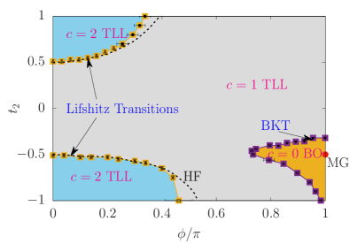
Figure 1: Phase diagram: Phases of the model in the $\phi-t_{2}$ plane ($t_{1}=1$). At $\phi=0$ the free Fermi system encounters Lifshitz transitions where the number of Fermi points changes. At $\phi\neq 0$ these evolve into central charge($c$) $=1$ and $=2$ Tomonaga Luttinger liquids(TLL). Near $\phi=\pi$ system undergoes a BKT transition from $c=1$ TLL to a gapped bond-ordered (BO) phase which spontaneously breaks lattice parity. At $\phi=\pi$ and $t_{2}=-0.5$ the system has an exactly solvable Majumdar-Ghosh (MG) point. The phase boundaries are determined studying the excitation gap. Dashed line represents the Lifshtiz transitions under the Hartree-Fock(HF) approximation (see text).

To uncover the physics of eqn. (2) we exploit the well known idea of interchanging statistics and interactions in 1D by introducing fractional Jordan-Wigner strings $K_{i}$, and defining operators

$$c_{i}=K_{i}a_{i},\quad c_{i}^{\dagger}=a_{i}^{\dagger}K_{i}^{\dagger}~{}~{}~{}{\rm with}~{}~{}~{}K_{i}=e^{-\mathbbm{i}\phi\sum_{j<i}n_{j}}.$$ (3)

Eq. 2 is thus mapped into a fermionic Hamiltonian

$${\cal H} = -\sum_{i}\left[t_{1}c_{i}^{\dagger}c_{i+1}+t_{2}e^{\mathbbm{i}\phi n_{i+1}}c^{\dagger}_{i}c_{i+2}\right]+{\rm h.c.}\,.$$ (4)

where $c_{i}^{\dagger},c_{i}$ are fermionic creation/annihilation operators at site $i$ obeying usual fermion anti-commutation algebra with the number density $n_{i}=c_{i}^{\dagger}c_{i}$. We note that while at $\phi=0,\pi$ both time-reversal (TRS) and parity symmetries are separately present, at any generic $\phi$ only a combination of both is a symmetry (see Supplemental Material (SM) , Sec. S1). While the first term in eqn. (4) is the nearest neighbor hopping, the second term contains the physics of correlated hopping between next-nearest-neighboring sites – fermions hop with a phase of $0$ ($\phi$) in absence (presence) of another fermion at the intermediate site. We note that a finite $t_{2}$ is crucial to realization of non-trivial phasesHao_PRA_2009; Hao_PRA_2012. Interestingly, correlated hoppings are known to arise in strongly correlated systems with constrained kinetic energies leading to frustration Foglio_PRB_1979; Arrachea_PRL_1994; Boer_PRL_1995; Vidal_PRB_2001.

Under the above non-local transformation the pseudofermion number density operator $N_{i}=a_{i}^{\dagger}a_{i}$ is equal to the fermion density operator $n_{i}=c_{i}^{\dagger}c_{i}$ and hence the filling fraction remains unchanged. Here, we shall concentrate on $1/2$ filling. In the remainder, we set $t_{1}=1$ and study the phase diagram as a function of $t_{2}$ and $\phi$. Eq. 4 is studied by analytical and numerical techniques.

Phase diagram:

Along the $\phi=0$ line the system reduces to that of free fermions with nearest and next-nearest-neighbor hopping with a single particle dispersion given by $E(k)=-2t_{1}\cos k-2t_{2}\cos 2k$ with $k\in[-\pi,\pi]$. There is a change in the number of the Fermi points as the system undergoes a Lifshitz transition at $t_{2}/t_{1}=\pm 0.5$. For $|t_{2}/t_{1}|>0.5(<0.5)$, there are four (two) Fermi points corresponding to the left most extremum of Fig. 1.

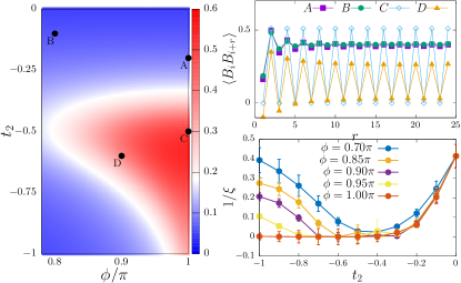
Figure 2: Gapped phase: (Left) $|O_{BO}|$ as a function of $\phi$ and $t_{2}$ in the gapped regime. (Top-Right) Dimer-dimer correlator $\langle B_{i}B_{i+r}\rangle$ and its behavior as a function of $r$ is shown at the marked points (A-D) on (Left). (Bottom-Right) Fitting $\langle B_{i}B_{i+r}\rangle\propto e^{-r/\xi}$; behavior of $1/\xi$ with $t_{2}$ for different values of $\phi$.

For $\phi=\pi$, we recover the familiar fermion to (hard-core) boson mapping evident from Eqs. 1 and 3. Thus we have a $1/2$-filled system of hard-core bosons with nearest and next nearest neighbor hoppings corresponding to the right extremum of Fig. 1. This is the easy-plane limit of the $J_{1}-J_{2}$ spin-$1/2$ chainMishra_PRB_2013; Dhar_PRA_2013. It has two phases– $c=1$ TLL for $t_{2}/t_{1}\gtrsim-0.3$ and a BO phase which spontaneously breaks inversion symmetry about a site which is characterised by a finite value of the order parameter $O_{BO}=\frac{1}{L}\sum_{i}(-1)^{i}B_{i},$ $B_{i}=\langle a^{\dagger}_{i}a_{i+1}+a^{\dagger}_{i+1}a_{i}\rangle$. Since the phase has a finite excitation gap, we expect it to be stable for small deviation of $\phi$ from $\pi$. DMRG results (Note1, Sec. S3) are plotted in Fig. 2 where we show both the BO order parameter as well as the two-point correlation function for the bond order. The lobe of BO order is roughly centered about $t_{2}/t_{1}=-0.5$ which is the Majumdar-Ghosh point Majumdar_JMP_1969; Majumdar_JMP_1969_2; Mishra_PRB_2013 for which the the BO ground state is exact at $\phi=\pi$. The structure of the lobe shows that at a fixed $0.79\pi\lesssim\phi<\pi$ there is a reentrant transition into a $c=1$ TLL as we tune $t_{2}/t_{1}$ from positive to negative. At $t_{2}/t_{1}=-\infty$ we have two decoupled chains which are in separate TLL phase. Turning on a positive $t_{1}$ destroys this state in favor of a bond order. However, we note that our calculations suggest that turning on a $\phi$ away from $\phi=\pi$ instead favors an instability to a $c=1$ TLL which competes with BO leading to a dome like structure.

Within a self-consistent Hartree-Fock (HF) treatment (Note1, Sec. S2)) of the correlated hopping term (for $\phi\neq 0$) by decoupling it in the $k$-mode density $\langle n(k)\rangle=\langle c^{\dagger}_{k}c_{k}\rangle$, we find that for $|t_{2}/t_{1}|<0.5$, the centre of the Fermi surface shifts away from zero for $\phi\neq 0,\pi$ due to the absence of TRS. For higher values of $|t_{2}/t_{1}|$ the HF calculations show that the Lifshitz transition continues into the interacting regime. The Lifshitz transitions of the effective HF Hamiltonian at any $\{t_{2},\phi\}$ traces a continuous quantum phase transition between the two gapless metallic phases (see the dashed curve in Fig. 1). However, not unexpectedly, this HF analysis breaks down in the gapped phase obtained in the vicinity of $\phi=\pi$.

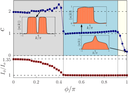
Figure 3: Lifshitz Transition: (Top) Central charge as a function of $\phi$ at $t_{2}=-0.75$ shows a transition from $c=2$ to a $c=1$ plateau. Fermion occupancy $\langle n(k)\rangle$ is shown as a function of $k$ at three representative values of $\phi$ as pointed. (Bottom) Variation of $I_{\phi}\equiv\int_{-\pi}^{\pi}\sin^{2}k\langle n(k)\rangle dk$ captures the Lifshitz transition. $I_{o}$ is the corresponding value for a half-filled Fermi sea at $t_{2}=0$.

The phase diagram (see fig. 1) for $\phi$ away from $\pi$, is occupied by two gapless TLLs. Interestingly, the HF theory does reproduce DMRG fermion occupancy of these phases remarkably well. In order to characterize the phases further, we calculate their central charges (using Calabrese-Cardy-formula for the entanglement entropy Calabrese_JPA_2009) and various correlation functions to determine the Luttinger parameters using DMRG results. Fig. 3 shows that even for finite $\phi$, the Lifshitz transition survives for the pseudofermions that separates the $c=1$ and the $c=2$ TLLs. The $c=1$ TLL can be understood within a low energy linearized (about the left and the right Fermi points ($k^{L}_{F}$ and $k^{R}_{F}$)) theory about the HF ground state given by $\mathcal{H}_{0}=-\mathbbm{i}\int dx\left[v_{f}^{R}\Psi_{R}^{\dagger}\partial_{x}\Psi_{R}-v_{f}^{L}\Psi_{L}^{\dagger}\partial_{x}\Psi_{L}\right]$ where, ($\Psi_{R},\Psi_{L}$) are left and right moving fermions and in the present case for $\phi,t_{2}\neq 0$ the corresponding Fermi velocities ($v^{R}_{f}$ and $v^{L}_{f}$) are different. Further Luttinger theorem restricts $k^{R}_{F}-k^{L}_{F}=\pi$ at half filling. While a similar construction can be obtained for the $c=2$ TLL by linearising about the four Fermi points and introducing two pairs of left and right moving fermions, characterizing this low energy theory requires characterizing the $2\times 2$ matrix Luttinger parameter sule2015determination, which we do not pursue here.

At finite $\phi>0$ and $t_{2}\neq 0$, none of TLLs have well defined quasi-particles–both of them being non-Fermi liquid metals. This is best seen by studying the effect of fluctuations over the HF theory Note1 within the framework of Abelian bosonization obtained by introducing the bosonized field $\Phi(x)$ and $\Theta(x)$ which obey the algebra $[\nabla\Phi(x),\Theta(y)]=[\nabla\Theta(x),\Phi(y)]=i\pi\delta(x-y)$. The effective low energy bosonized Hamiltonian for the $c=1$ TLL is given by

$$H= \frac{v_{f}}{2\pi}\int dx\left[\frac{1}{K}(\partial_{x}\Phi)^{2}+K(\partial_{x}\Theta)^{2}\right]$$

$$-\frac{W}{2\pi}\int dx\left[\partial_{x}\Phi\partial_{x}\Theta+\partial_{x}\Theta\partial_{x}\Phi\right]-\lambda\int dx\cos 4\Phi$$ (5)

where $v_{f}=\sqrt{(V_{F})^{2}-4\pi^{2}V^{2}}$ is the renormalised average Fermi velocity with $V_{F}=\frac{v_{f}^{R}+v_{f}^{L}}{2}$ and $W=\frac{v_{f}^{R}-v_{f}^{L}}{2}$. Here, $V$ and $\lambda$ arises due to interactions with $V$ and $\lambda$ being the forward and Umklapp scattering amplitude respectively given in terms of the microscopic correlated hopping parameters Note1. While $V$ kills the quasiparticles by renormalizing the Luttinger parameter $K$, $\lambda$ destabilizes the TLL leading to bond order. We use the relation between Luttinger parameter $K$ and the fermion two-point correlator

$$C(r):=\frac{1}{L}\sum_{i}\langle c^{\dagger}_{i}c_{i+r}\rangle\sim\frac{1}{r^{(K+1/K)/2}}$$ (6)

to extract $K$ from DMRG results. Parameters $K$ and $\lambda$ can also be calculated from the bosonized theory $K\left(=\sqrt{\frac{V_{F}-2\pi V}{V_{F}+2\pi V}}\right)$ . Away from the gapped region, where the Umklapp processes are small, the bosonization result compares well with DMRG results as seen in Fig. 4. For a fixed $t_{2}$, the Umklapp amplitude, $\lambda$, increases monotonically with $\phi$ such that the Umklapp scattering becomes important ultimately making the TLL unstable to a gapped BO phase. In the latter case, the bosonization values of $K,\lambda$ should be viewed as initial points of the RG flow as shown in Fig. 4. The instability to a gapped phase is also manifested through the Luttinger parameter reaching a critical value of $K=1/2$ as anticipated from a perturbative RG calculation. Away from the bond-ordered phase, for generic values of $2K>1$ our numerical calculation suggest a direct transition between the two TLL.

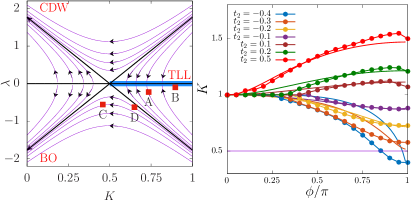
Figure 4: Bosonization and BKT Transition(Left) Luttinger parameter ($K$) and $\lambda$ calculated from the bosonization result for a set of parameters of $\{t_{2},\phi/\pi\}$ as shown by (A-D) in Fig. 2 (see near eqn. (5)) are shown by square points on the RG flow diagram of the BKT transition with TLL, BO and charge density wave (CDW) phases. $V$ and $\lambda$ are scaled by multiplicative prefactors of $\alpha/2\pi$ and $\alpha$ respectively where $\alpha\approx 0.3$. (Right) A plot of numerically extracted $K$ from the DMRG using $\langle c^{\dagger}_{i}c_{i+r}\rangle$ correlators and compared with the bosonization result.

Phase boundaries and the phase transitions :

In addition to the central charge, we use the excitation gap Mishra_PRB_2013: $\Delta_{L}=E(L,N+1)+E(L,N-1)-2E(L,N)$ (where $E(L,N)$ is the ground state energy for a system with $N$ particles on $L$ sites) to obtain the phase boundaries in Fig. 1 numerically. These calculations show that there are two types of phase boundaries denoting quantum phase transition between – (1) $c=1$ TLL (equivalently a powerlaw superfluid (SF)) to the symmetry broken bond ordered phase, and (2) $c=1$ and $c=2$ TLL phases. We now explore the nature these phase transitions.

Transition between the powerlaw SF to BO phase :

Our numerical calculations show that the entire phase boundary is captured by a BKT type phase transition (data collapse of gap scaling to BKT form shown in Note1). This is expected in the $\phi=\pi$ limit, where we have hard-core bosons and an application of XY duality in $(1+1)D$baeriswyl2005strong captures both the SF and the BO phases where extra Berry phases induce breaking of inversion symmetry in the BO phase Note1; sachdev2002quantum. To understand this transition to general $\phi$, it is convenient to use the bosonized field theory by writing down the Euclidean action corresponding to eqn. (5). The effect of finite $\phi$ is to provide a “boosted” field theory where the effect of the “boost” can then be gauged away Ray_AP_2017. The Umklapp scattering then drives the BO instability gapping out the TLL as can be seen in the behavior of the Luttinger parameter (see Fig. 4). The corresponding RG flows based on the Sine-Gordon theory (Fig. 4) effectively capture the phase transition along with the phases.

Transition between $c=1$ and $c=2$ TLL :

Our central charge calculations suggest that the Lifshitz transition for finite $\phi$ from $c=1$ CFT (TLL with two Fermi points) to $c=2$ CFT (TLL with four Fermi points) is a rather sudden one when compared to the BKT transition. However, crucially there is no local real space order parameter based description for this quantum phase transition which then requires careful examination regarding its nature. The HF band structure suggests that the low energy modes near this transition contains the linearly dispersing left, $\psi_{L}$, and right, $\psi_{R}$, fermions along with quadratically dispersing holes of the central lobe, $\psi_{c}$. At $\phi=0$, these modes are non interacting and the transition at $t_{2}/t_{1}=-0.5$ is given by a dynamical exponent $z=2$ theory where changing $t_{2}$ has the primary effect of changing the hole chemical potential leading to finite density of holes. Strictly speaking because of the overall Luttinger theory this leads to renormalisation of the Fermi-velocities of both $\psi_{L}$ and $\psi_{R}$, but, they lead to innocuous renormalisation of various quantities as these modes do not couple to $\psi_{c}$. Assuming that the above picture holds at least for finite $\phi$, we bosonize the left and right fermions to get the following effective low energy Hamiltonian $\mathcal{H}=H+H^{\prime}$, where where $H$ is given by eqn. (5) and

$$H^{\prime}=\int dx~{}\psi_{c}^{\dagger}\left[\frac{\partial_{x}^{2}}{2m^{*}}-\mu\right]\psi_{c}+\int dx\left(g_{1}\partial_{x}\Phi+g_{2}\partial_{x}\Theta\right)\psi^{\dagger}_{c}\psi_{c}.$$ (7)

The first term in $H^{\prime}$ is the free action of the quadratically dispersing fermionic holes with effective mass $m^{*}$ and chemical potential $\mu$ which is zero at $t_{2}/t_{1}=-0.5$ and increases (decreases) for $t_{2}/t_{1}<-0.5(>-0.5)$ and thereby capturing the HF phase transition. $g_{1}$ and $g_{2}$ are two symmetry allowed coupling constants (details in Note1, Sec. S5) which go to zero as $\phi\rightarrow 0$. Perturbative one-loop RG calculations around the $\mu=g_{1}=g_{2}=0$ shows that this critical point is stableNote1. Similar field theories are suggested in context of multimode wiresSitte_PRL_2009; Meng_PRB_2011; Rodney_PRB_2013; However, a full characterization requires further studies. In absence of any local order-parameter, we define “moment-of-inertia” of the Fermi sea as $\int n(k)(\sin(k))^{2}dk$ and find that it shows a smooth variation across the Lifshitz transition (see Fig. 3). Remarkably just tuning the statistical phase of pseduofermions can mediate this transition between two non-Fermi liquids neither of which has low energy quasi-particles.

Summary and outlook :

We have shown that a simple quadratic system of pseudofermions hopping on $1$D lattice with nearest and next nearest neighbor hopping following fractionalized algebra (eq. 1), has a rich phase diagram with gapless TLL phases and gapped BO phases which can be accessed by tuning the statistical parameter and ratio of lattice hopping. The phase transitions include a BKT transition between a $c=1$ TLL and a BO phase as well as a possible continuous Lifshitz phase transition between two TLLs with central charges $c=1$ and $2$. The fractionalized algebra is naturally obtained in a system of fermions with correlated hopping. Recent proposals Liberto_PRA_2014; Cardarelli_PRA_2016; Ghosh_PRA_2017 of generating such off-site correlated hopping in fermionic ultra-cold atoms can potentially realise the above quadratic system of such particles enabling us to provide more comprehensive understanding of unconventional phases and phase transitions in lower dimensional systems.

Acknowledgements :

We acknowledge fruitful discussions with Diptiman Sen, H.R. Krishnamurthy, Krishnendu Sengupta, Subroto Mukerjee, Smitha Vishveshwara, R. Loganayagam, Avinash Dhar, R. Moessner, Tapan Mishra, Arun Parmakanti and Sumilan Banerjee. A. A. and S. B. acknowledges MPG for funding through the Max Planck Partner group on strongly correlated systems at ICTS. S. B. acknowledges SERB-DST (India) for funding through project grant No. ECR/2017/000504. V.B.S. acknowledges support from DST(India). DMRG calculations are performed using ITensor Itensor. The numerical calculations were done on the cluster Mowgli, boson and zero at the ICTS and Sahastra at IISc. We acknowledge ICTS and the discussion meeting “New questions in quantum field theory from condensed matter theory” during which some of these ideas originated.

Supplemental Material

for

Statistics-tuned phases of pseudofermions in one dimension

Adhip Agarwala, Gaurav Kumar Gupta, Vijay B. Shenoy and Subhro Bhattacharjee

S1 Microscopic Hamiltonian : symmetries and the free fermion limit ($\phi=0$)

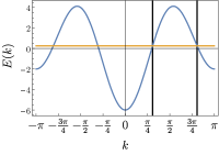
(a) Dispersion when $\phi=0$ and $t_{2}=2$

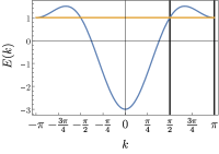
(b) Dispersion when $\phi=0$ and $t_{2}=0.5$

(c) Dispersion when $\phi=0$ and $t_{2}=-0.5$

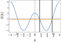
(d) Dispersion when $\phi=0$ and $t_{2}=-2$

Supplementary Figure S1: (a) Schematic figure describing the Hamiltonian. (b)-(e) Single particle dispersion for the fermion problem in $\phi=0$ limit. For $t_{2}>0$ depending on the value of $t_{2}$ we can either have two (for $|t_{2}|<\frac{1}{2}$) Fermi points (at $\pm\pi/2$) or four (for $|t_{2}|>\frac{1}{2}$) Fermi points.

S1.1 Symmetries

The one dimensional chain with nearest and next nearest neighbor coupling can be alternatively thought of as a zig-zag ladder (fig. S1) with the following symmetries : (1) Lattice translation by unit lattice spacing of the one dimensional chain, $T_{x}$, and (2) Combination of time-reversal (${\cal T}$) and parity ${(\cal P)}$ as $\mathcal{Q}=\mathcal{P}\mathcal{T}$.

Under $T_{x}$, the fermions transform as,

$${T_{1}}c_{i}{T_{1}}^{-1}=c_{i+1},\;\;\;\ {T_{-1}}c_{i}{T_{-1}}^{-1}=c_{i-1},\quad{T_{1}}c_{L}{T_{1}}^{-1}=c_{1},\;\;\;\ {T_{-1}}c_{1}{T_{-1}}^{-1}=c_{L}.$$ (S1.8)

Note that we have we have $L$ sites labeled $\{1\ldots L\}$ where $L$ is taken to be an even number. Thus on the pseudofermions, $a_{i}$, translations act as

$${T_{1}}a_{i}{T_{1}}^{-1}={T_{1}}K^{\dagger}_{i}c_{i}{T_{1}}^{-1}=e^{-i\phi n_{1}}K^{\dagger}_{i+1}c_{i+1}=e^{-i\phi N_{1}}a_{i+1}$$ (S1.9)

$${T_{-1}}a_{i}{T_{-1}}^{-1}={T_{-1}}K^{\dagger}_{i}c_{i}{T_{-1}}^{-1}=e^{i\phi n_{L}}K^{\dagger}_{i-1}c_{i-1}=e^{i\phi N_{L}}a_{i-1}.$$ (S1.10)

Under $\mathcal{T}$ and $\mathcal{P}$, the fermion operators transform in the following way

$${\cal T}c_{i}{\cal T}^{-1}=c_{i},~{}~{}~{}~{}~{}~{}~{}~{}~{}~{}~{}~{}~{}~{}{\cal T}c^{\dagger}_{i}{\cal T}^{-1}=c^{\dagger}_{i}$$ (S1.11)

$${\cal P}c_{i}{\cal P}^{-1}=c_{L-i+1}~{}~{}~{}~{}~{}~{}~{}~{}~{}~{}~{}{\cal P}c^{\dagger}_{i}{\cal P}^{-1}=c^{\dagger}_{L-i+1}$$ (S1.12)

This results in the following transformation for the pseudofermion operators $a_{i}$,

$${\cal T}a_{i}{\cal T}^{-1} = {\cal T}K^{\dagger}_{i}c_{i}{\cal T}^{-1}=K_{i}c_{i}$$ (S1.13)

$${\cal P}a_{i}{\cal P}^{-1} = {\cal P}K^{\dagger}_{i}c_{i}{\cal P}^{-1}=e^{i\phi{\cal N}}K_{L-i+2}c_{L-i+1}=e^{i\phi{\cal N}}K_{L-i+1}c_{L-i+1}$$ (S1.14)

where ${\cal N}=\sum_{i}N_{i}=\sum_{i}n_{i}$. Thus, under the combination of these symmetries, $\mathcal{Q}$, the $a_{i}$s transform as :

$${\cal Q}a_{i}{\cal Q}^{-1}=e^{-i\phi{\cal N}}a_{L-i+1}~{}~{}~{}~{}~{}~{}~{}~{}~{}~{}~{}~{}~{}~{}~{}~{}{\cal Q}a^{\dagger}_{i}{\cal Q}^{-1}=a^{\dagger}_{L-i+1}e^{i\phi{\cal N}}$$ (S1.15)

S1.2 Free fermions at $\phi=0$

The free fermion dispersion at any value of $t_{2}$ is given by,

$$E(k)=-2t_{1}\cos k-2t_{2}\cos 2k$$ (S1.16)

The dispersions for few representative values of $t_{2}$ (keeping $t_{1}=1$) are shown in Fig. S1. For $-1/2<t_{2}<1/2$, there are two Fermi points at $k=\pm\pi/2$. For $|t_{2}|>1/2$, there are $4$ Fermi points ($k^{R\pm}_{F},k^{L^{\pm}}_{F}$) given by

$${\rm For}~{}t_{2}>1/2:~{}~{}~{}\quad k^{R+}_{F}=\arccos\left(\frac{-1}{2\sqrt{2}t_{2}}\right)-\frac{\pi}{4},~{}~{}k^{L+}_{F}=k^{R+}_{F}+\frac{\pi}{2},~{}~{}k^{R-}_{F}=-k^{L+}_{F},~{}~{}k^{L-}_{F}=-k^{R+}_{F}$$ (S1.17)

$${\rm For}~{}t_{2}<1/2:~{}~{}~{}\quad k^{R+}_{F}=\arccos\left(\frac{1}{2\sqrt{2}|t_{2}|}\right)+\frac{\pi}{4},~{}~{}k^{L+}_{F}=k^{R+}_{F}-\frac{\pi}{2},~{}~{}k^{R-}_{F}=-k^{L+}_{F},~{}~{}k^{L-}_{F}=-k^{R+}_{F}$$ (S1.18)

Therefore at $\phi=0$, as a function of $t_{2}$ we have Lifshitz transition akin to the tuning of the chemical potential.

Fermi Velocity :

The Fermi velocity can be determined by the slope of the dispersing band at the Fermi points. For $|t_{2}|<\frac{1}{2}$ the Fermi points remain pinned at $k_{F}=\pm\frac{\pi}{2}$ and the corresponding Fermi velocities continue to be $v_{F}=\frac{\partial E(k)}{\partial k}|_{k=k_{F}}=\pm 2t_{1}$. For $|t_{2}|>\frac{1}{2}$ the Fermi velocities at the four Fermi points depend on $t_{2}$ and are given by $\left(2t_{1}\sin k^{R/L\pm}_{F}+4t_{2}\sin 2k^{R/L\pm}_{F}\right)$ respectively.

S2 Hartree-Fock theory

Rewriting the fermionic Hamiltonian as a sum of free quadratic part and an interacting quartic part, we get

$$H=H_{0}+H_{int}$$ (S2.19)

where in the momentum space $k\in[-\pi,\pi]$, $H_{0}=\sum_{k}\varepsilon_{0}(k)c^{\dagger}_{k}c_{k}$ with $\varepsilon_{0}(k)=-2[t\cos(k)+t_{2}\cos(2k)]$ being the bare dispersion and

$$H_{int}=-t_{2}\sum_{k_{1},k_{2},k_{3},k_{4}}\delta(k_{1}+k_{2}-k_{3}-k_{4})[(e^{i\phi}-1)e^{i(-k_{2}+k_{3}+2k_{4})}]c^{\dagger}_{k_{1}}c^{\dagger}_{k_{2}}c_{k_{3}}c_{k_{4}}+{\rm h.c.}$$ (S2.20)

Now concentrating on the Hartree-Fock decomposition of the interactions as

$$c^{\dagger}_{k_{1}}c^{\dagger}_{k_{2}}c_{k_{3}}c_{k_{4}}\rightarrow-\langle c^{\dagger}_{k_{1}}c_{k_{3}}\rangle c^{\dagger}_{k_{2}}c_{k_{4}}-c^{\dagger}_{k_{1}}c_{k_{3}}\langle c^{\dagger}_{k_{2}}c_{k_{4}}\rangle+\langle c^{\dagger}_{k_{1}}c_{k_{4}}\rangle c^{\dagger}_{k_{2}}c_{k_{3}}+c^{\dagger}_{k_{1}}c_{k_{4}}\langle c^{\dagger}_{k_{2}}c_{k_{3}}\rangle$$ (S2.21)

we get

$$H_{HF} = \sum_{k}\{\varepsilon_{0}(k)+A(k)+B+C(k)\}c^{\dagger}_{k}c_{k}$$ (S2.22)

where,

$$A(k) = {2}t_{2}\sum_{k^{\prime}}\{(e^{i\phi}-1)e^{i(k+k^{\prime})}+h.c.\}\langle n(k^{\prime})\rangle$$ (S2.23)

$$B = -2t_{2}\sum_{k^{\prime}}\{\cos(\phi+2k^{\prime})-\cos(2k^{\prime})\}\langle n(k^{\prime})\rangle$$ (S2.24)

$$C(k) = -2t_{2}\{\sum_{k^{\prime}}\langle n(k^{\prime})\rangle\}\{\cos(\phi+2k)-\cos(2k)\}$$ (S2.25)

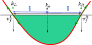
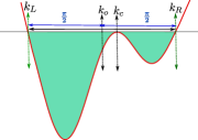
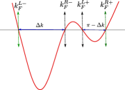
Supplementary Figure S2: (a) The Hartree-Fock (HF) dispersion is schematically shown in the TLL $c=1$ phase. (b) Schematic of the HF dispersion at a “Lifshitz” transition when the system undergoes a gapless-gapless transition between TLL ($c=1$) and TLL ($c=2$) phase. (c) Schematic of the HF dispersion when the system is in $c=2$ TLL phase.

Solving this self-consistently for $\langle n(k)\rangle=\langle c_{k}^{\dagger}c_{k}\rangle$ produces the renormalised single particle dispersion for different values of the parameters. The general structure of the HF band is shown schematically in Fig. S2 when the system is in either of the two kinds of TLL phases and at a Lifshitz transition. Fig. S3 shows the HF fermionic occupation for representative points in the parameter space. This should be compared with the DMRG results as shown in Fig. S11. The HF theory clearly captures the gapless phases in $c=1$ and $c=2$ TLL regimes. It also captures the associated Fermi momenta and Lifshitz transitions as seen by a dashed line in Fig. 1 of the main text.

Supplementary Figure S3: $\langle n(k)\rangle$ as a function of $k$ and $t_{2}$ for different values of $\phi$ using a self consistent mean field theory. The values of $\phi$ are $0.0,1.0,2.0$ and $3.0$.

In the $c=1$ phase the center of the Fermi sea is shifted and the occupied states have momenta $k_{o}-\frac{\pi}{2}\leq k\leq k_{o}+\frac{\pi}{2}$ where the shift of the centre, $k_{o}$ is given by

$$\sin(k_{o})=\frac{4t_{2}}{\pi}\sin\left(\frac{\phi}{2}\right)\cos\left(\frac{\phi}{2}+2k_{o}\right)$$ (S2.26)

In this phase, the HF Hamiltonian can be linearised about the two Fermi points by introducing the left and right moving fermion fields, $\Psi_{L}$ and $\Psi_{R}$ respectively to get linearised Hamiltonian in real space as

$$\mathcal{H}_{0}=i\int dx\left[v_{f}^{R}\Psi_{R}^{\dagger}\partial_{x}\Psi_{R}-v_{f}^{L}\Psi_{L}^{\dagger}\partial_{x}\Psi_{L}\right]$$ (S2.27)

where $v_{f}^{R}(v_{f}^{L})$ are the Fermi velocities for the right and left moving fermions respectively which are given by :

$$v^{R}_{f}=\frac{\partial\varepsilon_{k}}{\partial k_{f}^{R}}~{}~{}~{}~{}~{}v^{L}_{f}=-\frac{\partial\varepsilon_{k}}{\partial k^{L}_{f}}$$ (S2.28)

Due to breaking of the time-reversal symmetry – the Fermi sea center gets shifted from $k=0$ ($\equiv k_{o}$) and the two Fermi velocities at the Fermi points can in general be different. The variation of Fermi velocities and $k_{o}$ as a function of few parameters is shown in Fig. S4.

Supplementary Figure S4: The right and left Fermi velocities ($v^{R}_{f}$ and $v^{L}_{f}$) as a function of $\phi$ for $t_{2}=-0.01$, $t_{2}=-0.1$ and $t_{2}=-0.3$. Notice that the right and left velocities are different. The right most figure shows the comparison of shifted center of the Fermi sea $\equiv k_{o}$ from both HF and the DMRG study (see eqn. (S3.36)) for various values of $t_{2}$ and as a function of $\phi$.

S3 Details of the numerical DMRG calculations

Here we provide various details of our DMRG calculations including the comparison with exact diagonalisation (ED) results for small systems.

S3.1 Determination of the phase diagram : Excitation gap, fidelity and central charge

S3.1.1 Excitation gap

$\Delta_{L}$ is the gap to single particle excitation defined as

$$\Delta_{L}=E(L,N+1)+E(L,N-1)-2E(L,N)$$ (S3.29)

where $E(L,N)$ is the ground state energy for a system with $N$ fermions on $L$ sites. In the gapless regime $\Delta_{L}$ scales as $1/L$ (see Fig. S5) and reaches $zero$ while in the gapped regime the value saturates to a finite value $\equiv\Delta_{\infty}$. Variation of $\Delta_{\infty}$ as a function of $t_{2}$ for various values of $\phi$ is shown in Fig. S5 which is also the regime shown in Fig. 2 of the main text.

BO phase and associated BKT transition :

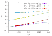
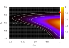
Supplementary Figure S5: (a) Behavior of $\Delta_{L}$ at few parameters of $\{t_{2},\phi\}$ as a function of $1/L$. For gapless phases $\Delta_{L}$ reaches $zero$ as a function of $1/L$ and saturates to a finite value ($\equiv\Delta_{\infty}$) for gapped regime. (b) Behavior of $\Delta_{\infty}$ in the gapped regime is shown as a function of $t_{2}$ for few values of $\phi$ and in the extended region (c).

The transition between the $c=1$ TLL and the BO phase is expected to be of BKT type (see main text). In order to pin the phase boundary, earlier works Dalmonte_PRB_2015; Carrasquilla_PRA_2013 have shown that behavior of correlation functions, fidelity etc. may have significant errors near the transition. Instead, an alternate prescription of a data collapse of $\Delta_{L}$ with a scaling form of the correlation length provides a rather accurate estimate. Briefly, the method entails that the variation of $\Delta_{L}L$ with $\log L-\frac{a}{\sqrt{V-V_{c}}}$ follows a universal behavior, where $V$ is a tuning parameter and $V_{c}$ is the critical value. Defining $x_{L}=\log L-\frac{a}{\sqrt{V-V_{c}}}$, values of $\Delta_{L}L$ and corresponding $x_{L}$s for various $L$s and $V$s near $V_{c}$ (in the gapped regime) can be fitted to a curve. Treating $a$ and $V_{c}$ as variational parameters, the least square fitting error is minimized to optimize $a,V_{c}$. A representative estimation of the same is shown in Fig. S6. This procedure is used to for determining the gapless-gapped transition boundary as shown in the Fig. 1 of the main text.

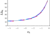
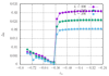
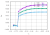
Supplementary Figure S6: (a-b) Best obtained collapse of $\Delta_{L}L$ and $x_{L}=\log L-\frac{a}{\sqrt{\phi-\phi_{c}}}$ by variation of $a,\phi_{c}$. The estimation of $a,\phi_{c}$ is done by minimizing the fitting error. Here, this is done for the transition from gapless to gapped point as a function of $\phi$ for $t_{2}=-0.70$. (c-d) Behavior of $\Delta_{L}$ as a function of $t_{2}$ across the gapless-gapless transition for $\phi/\pi=0.28$ and $\phi/\pi=0.42$ for three different values of $L=200,240,300$. Notice that unlike the gapless-gapped transition, for any finite $L$, $\Delta_{L}$ shows a jump to $zero$ at the Lifshitz transition.

Behavior of excitation gap in the TLL phases and near the metal-metal transition :

Behavior of $\Delta_{L}$ as a function of $t_{2}$ across the gapless-gapless transition for $\phi/\pi=0.28$ and $\phi/\pi=0.42$ for three different values of $L=200,240,300$ is shown in Fig. S6. Note the rather abrupt jump in $\Delta_{L}$ to $zero$ unlike the gapless-gapped transition. This jump points out the boundary of the transition between the $c=1$ and $c=2$ phase.

S3.1.2 Fidelity

Given two groundstate wavefunctions evaluated at parameters $\lambda$ and $\lambda+d\lambda$, the fidelity susceptibility is given by Gu_IJMB_2010

$$\chi_{F}(\lambda)=\lim_{d\lambda\rightarrow 0}\frac{-2\log(|\langle\psi(\lambda+d\lambda)|\psi(\lambda)\rangle|)}{(d\lambda)^{2}}.$$ (S3.30)

Signatures in $\chi_{F}$ signal phase transitions. Fig. S7 shows the behavior of $\chi_{F}$ while going from gapless to gapped regime (a-b) and between gapless to gapless regime (c-d) for different system sizes. Note that $\chi_{F}$ behaves rather differently at the two kinds of transition. In order to corroborate our DMRG results we compare the results for small system sizes with exact diagonalization (ED) studies. Some representative figures are shown in Fig. S8.

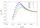
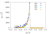
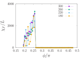
Supplementary Figure S7: Fidelity susceptibility $\chi_{F}$ : (a) as a function of $t_{2}$ at $\frac{\phi}{\pi}=0.8732$ and (b-d) as a function of $\phi/\pi$ for $t_{2}=-0.46,1.00$ and $0.7$. The humps signal phase transitions.

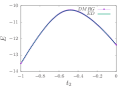
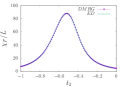
Supplementary Figure S8: Ground state energy and fidelity susceptibility $\chi_{F}/L$ as a function of $t_{2}$ for $\phi/\pi=0.859$ for a system size $L=20$ under open-boundary condition, both using exact diagonalization and DMRG.

S3.1.3 Entanglement Entropy and Central Charge

In DMRG we work with open-boundary condition – here it is known from Cardy-Calabrese formula, that entanglement entropy of a subsystem size $l$ as a function of $l/L$ can be fitted to the following form Calabrese_JPA_2009

$$S(l)=\frac{c}{6}\ln[\frac{L}{\pi}\sin(\frac{\pi l}{L})]+\ldots$$ (S3.31)

to estimate $c$, the central charge.

Central charge at the BKT transition :

Behavior of central charge across the BKT transition is shown in Fig. S9 for few parameters where central charge changes from $1$ to $zero$.

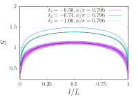
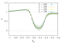
Supplementary Figure S9: (a) Entanglement entropy for three different parameters of $t_{2},\phi$ as a function of bond length $l/L$ for $L=300$. The central charge($c$) is estimated using the Cardy-Calabrese formula. Variation of $c$ for four different system sizes as a function of $\phi$ for $t_{2}=-0.60$ (b) and as a function of $t_{2}$ for $\phi/\pi=0.891$ $(c)$.

Central charge at the gapless-gapless transition :

Behavior of central charge transition at gapless-gapless transitions are shown in Fig. S10. Note the abrupt change in $c$ in contrast to the smooth variation in $c$ for gapless-gapped transition.

Supplementary Figure S10: The variation of central charge $c$ as a function of $t_{2}$ for $\phi/\pi=0.159$ (a) and $\phi/\pi=0.18$ (b) showing a gapless-gapless transition between the $c=1$ and $c=2$ phases. (c-d) Comparison of $c$ evaluated using DMRG and correlation matrix at the free fermionic limit ($\phi$=0) as a function of $t_{2}$ for different system sizes. (d) shows dependence of $c$ evaluated at $t_{2}=-1,\phi=0$ for different system sizes and bond-dimension. Even at the free fermion limit, to capture the $c=2$ phase one needs to have a significantly large bond-dimension.

The behavior of $c$ near $\phi=0$ limit can be understood by comparing the results of DMRG with that obtained by calculating entanglement entropy using correlation matrix Chung_PRB_2001; Cheong_PRB_2004; Peschel_JPA_2003; Vidal_PRL_2003 ($C_{ij}=\langle c^{\dagger}_{i}c_{j}\rangle$ where the expectation is taken over the occupied states). The value of central charge calculated using this is shown in Fig. S10.

S3.2 Characterisation of the phases

S3.2.1 Fermionic occupation number in momentum space

The fermion mode occupancy $\langle n(k)\rangle=\langle c_{k}^{\dagger}c_{k}\rangle$ is shown in Fig. S11. While the similarity with the HF results is quite striking, we note that there is no jump discontinuity for the fermion occupation as this is a TLL. $\langle n(k)\rangle$ allows us to calculate “moment of intertia” of the Fermi sea given by

$$I=\int dk\langle n(k)\rangle(\sin(k))^{2}$$ (S3.32)

the variation of which as a function of $t_{2}$ for different values of $\phi$ is shown in Fig. S12. While the gapless to gapless transition is characterized by a change in $I$, the gapless to gapped transition shows no such variation.

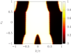
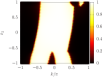
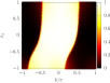
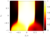
Supplementary Figure S11: $\langle n(k)\rangle$ as a function of $k$ and $t_{2}$ for different values of $\phi=0.0,1.0,2.0,3.0$ via DMRG calculations.

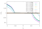
Supplementary Figure S12: Variation of $I=\int dk\langle n(k)\rangle(\sin(k))^{2}$ with $t_{2}$ for different values of $\phi$. $I_{o}$ is the corresponding value for a half-filled Fermi sea at $t_{2}=0$.

S3.2.2 Bosonic occupation number in momentum space

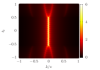
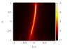
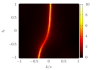
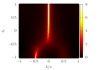
Supplementary Figure S13: Bosonic $\langle n_{b}(k)\rangle$ as a function of $k$ and $t_{2}$ for different values of $\phi=0.0,1.0,2.0$ and $3.0$.

While most of our discussion of the gapless phases has been in terms of TLL, a quantity worth investigating is the expectation value of $\langle n^{b}_{k}\rangle\equiv\langle b^{\dagger}_{k}b_{k}\rangle$ which is expectation of each of the occupancy of the $k^{th}$ mode in bosonic language. Fig. S13 shows this for various values of $\phi$ and $t_{2}$ ($\langle n_{b}(k)\rangle=\langle b^{\dagger}(k)b(k)\rangle=\frac{1}{L}\sum_{i,j}\exp{ik(i-j)}\langle S^{+}_{i}S^{-}_{j}\rangle$). Clearly the TLL phase is equivalently a power law superfluid as pointed in the main text. The shifted center of the Fermi sea in TLL manifests as again a shifted $k$ point where the superfluid $\langle n_{b}(k)\rangle$ peaks.

S3.2.3 Characterisation of the $c=1$ TLL phase : Luttinger Parameters from DMRG study

To characterise the $c=1$ TLL, it is particularly useful to calculate the fermion-fermion correlation function in this system. In the regime when the $\langle n(k)\rangle$ shows “two” Fermi surfaces – i.e. $c=1$ TLL

$$C(r)=\frac{1}{L}\sum_{i}\langle c^{\dagger}_{i}c_{i+r}\rangle=\frac{1}{2\pi}\int_{-\pi}^{\pi}dk\langle n(k)\rangle e^{-ikr}.$$ (S3.33)

For the case when $\phi=0$ and $-0.5\leq t_{2}\leq 0.5$, such that there is a filled Fermi sea between $-\frac{\pi}{2}\leq k\leq\frac{\pi}{2}$,

$$C(r)=\frac{\sin(\pi r/2)}{\pi r}.$$ (S3.34)

For $|t_{2}|\geq 0.5$, $C(r)$ shows an oscillating behavior due to new Fermi wavevectors. In particular, for $t_{2}<-0.5$ we have two Fermi seas, one between $k^{L+}_{F}\leq k\leq k^{R+}_{F}$ and the other between $k^{L-}_{F}\leq k\leq k^{R-}_{F}$. In this regime

$$C(r)=\frac{2\cos\left(\arccos(\frac{t_{1}}{2\sqrt{2}|t_{2}|})r\right)\sin(\frac{\pi}{4}r)}{\pi r}.$$ (S3.35)

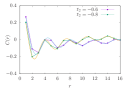
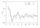
Supplementary Figure S14: $C(r)$ has a function of $r$ for $\phi=0$ for different values of $t_{2}$. The numerical values from DMRG are the points. The continuous lines are the expressions shown near eqn. (S3.35) for appropriate parameters.

Similar calculations can be done for for $t_{2}>0.5$ (See Fig. S14). In presence of the interactions ($\phi\neq 0$) the long wavelength scaling of the correlation function changes from $\sim\frac{1}{r}$ to $\frac{1}{r^{\eta}}$ where $\eta$ can be related to the Luttinger parameter Sachdev_book. In $c=1$ TLL, which is the region of $-0.5<t_{2}<0.5$ and when $\phi\neq 0$, we fit $C(r)$ to a functional form

$$C(r)\sim\frac{\cos(k_{o}x)\sin(\frac{\pi}{2}x)}{\pi x^{\eta}}$$ (S3.36)

where both $\eta$ and $k_{o}$ are fitting parameters. The intention is to capture the shift in the Fermi sea ($k_{o}$) and the Luttinger parameter ($K$) where $K$ is related to $\eta$ via $\eta=\frac{1}{2}(K+\frac{1}{K})$. A comparison of $k_{o}$ obtained by above and the Hartree-Fock solution is shown in Fig. S4 for bench marking.

S4 Bosonization for the $c=1$ TLL

The Hartree-Fock treatment as discussed above leads to a dispersion as schematically shown in Fig. S2(a). In general this free theory has two Fermi points centered about $k_{o}\neq 0$ and the Fermi velocities are not equal. A bosonization treatment Sachdev_book in terms of bosonic fields $\{\Theta,\Phi\}$ satisfying

$$[\nabla\Phi(x),\Theta(y)]=[\nabla\Theta(x),\Phi(y)]=i\pi\delta(x-y)$$ (S4.37)

leads to the following free theory linearised about the HF ground state

$$\tilde{\mathcal{H}}_{0}=\frac{V_{F}}{2\pi}\int dx\left[(\partial_{x}\Phi)^{2}+(\partial_{x}\Theta)^{2}\right]+\frac{W}{2\pi}\int dx\left[\partial_{x}\Phi\partial_{x}\Theta+\partial_{x}\Theta\partial_{x}\Phi\right]$$ (S4.38)

where $V_{F}=\frac{v_{f}^{R}+v_{f}^{L}}{2}$ and $W=\frac{v_{f}^{R}-v_{f}^{L}}{2}$. The interaction term is given by,

$$\tilde{H}_{int}=-t_{2}\sum_{k_{1},k_{2},k_{3},k_{4}}\delta_{k_{1}+k_{2}-k_{3}-k_{4}}(e^{i\phi}-1)e^{i(-k_{2}+k_{3}+2k_{4})}\left[:c^{\dagger}_{k_{1}}c_{k_{4}}::c^{\dagger}_{k_{2}}c_{k_{3}}:-:c^{\dagger}_{k_{1}}c_{k_{3}}::c^{\dagger}_{k_{2}}c_{k_{4}}:\right]+h.c.$$ (S4.39)

where the normal ordering is done about the HF ground state. Identifying the slow modes, one finds two essential scattering contributions – (i) Forward scattering and (ii) Umklapp scattering. Defining $\rho_{R}(q)=\sum_{q_{1}}:c^{\dagger}_{q_{1}R}c_{q_{1}+qR}:$ and $\rho_{R}(x)=\sum_{q}e^{iqx}\rho_{R}(q)$, forward scattering contribution is

$$\tilde{H}^{Fow}_{int}=V\int dx\Big{(}(\rho_{R}+\rho_{L})^{2}-(\rho_{R}-\rho_{L})^{2}\Big{)}=V\int dx\left[(\partial_{x}\Phi)^{2}-(\partial_{x}\Theta)^{2}\right]$$ (S4.40)

where $V=4t_{2}(\cos(\phi+2k_{o})-\cos(2k_{o}))$. For Umklapp process the contribution is

$$\tilde{H}_{int}^{Ump} = -\lambda\int dx\cos 4\Phi$$ (S4.41)

where $\lambda=-2V$. Gathering all the terms we get the bosonized Hamiltonian to be

$$H=\frac{v_{f}}{2\pi}\int dx\left[\frac{1}{K}(\partial_{x}\Phi)^{2}+K(\partial_{x}\Theta)^{2}\right]-\frac{W}{2\pi}\int dx\left[\partial_{x}\Phi\partial_{x}\Theta+\partial_{x}\Theta\partial_{x}\Phi\right]-\lambda\int dx\cos 4\Phi$$ (S4.42)

where the renormalised average Fermi-velocity is given by $v_{f}=\sqrt{(V_{F})^{2}-4\pi^{2}V^{2}}$ and the Luttinger parameter is given by

$$K=\sqrt{\frac{V_{F}-2\pi V}{V_{F}+2\pi V}}.$$ (S4.43)

$V$ and $\lambda$ both go to zero at $\phi=0$ and hence at this point, $K=1$. Also, as expected, $W=0$ in this limit. This is nothing but the free fermions. To understand the effect of the other terms, we derive the corresponding real time action which is given by

$$\mathcal{S}=\frac{1}{2\pi v_{f}K}\int dtdx\left[\left(\partial_{t}\Phi+\frac{w}{2}\partial_{x}\Phi\right)^{2}-v_{f}^{2}(\partial_{x}\Phi)^{2}\right]+\lambda\int dt~{}dx\cos 4\Phi$$ (S4.44)

where $w=W/\Delta\tau$ where the limit is taken such that $w$ is constant. The effect of the “boost” can then be gauged away Ray_AP_2017 after which we can wick rotate it to imaginary time to get the Euclidean action

$$\mathcal{S}_{E}=\frac{1}{2\pi v_{f}K}\int d\tau dx\left[\left(\partial_{\tau}\Phi\right)^{2}+v_{f}^{2}(\partial_{x}\Phi)^{2}\right]-\lambda\int d\tau~{}dx\cos 4\Phi.$$ (S4.45)

S5 Details of the field theoretic calculations for the phase transitions

S5.1 Field theory at the gapless-gapless transition

Within HF, the gapless-gapless transition is a Lifshitz transition (see schematic Fig. S2(b)). The effective Hamiltonian here is given by

$${\cal H} = \frac{v_{f}}{2\pi}\int dx\left[\frac{1}{K}(\partial_{x}\Phi)^{2}+K(\partial_{x}\Theta)^{2}\right]-\frac{W}{2\pi}\int dx\left[\partial_{x}\Phi\partial_{x}\Theta+\partial_{x}\Theta\partial_{x}\Phi\right]-\lambda\int dx\cos 4\Phi$$ (S5.46)

$$+ g_{1}\int dx[\psi^{\dagger}_{c}(x)\psi_{c}(x)\partial_{x}\Phi]+g_{2}\int dx[\psi^{\dagger}_{c}(x)\psi_{c}(x)\partial_{x}\Theta]+\int dx\psi^{\dagger}_{c}[\frac{\partial^{2}_{x}}{2m*}-\mu]\psi_{c}$$

where

$$g_{1} = -4t_{2}\left(\{\cos(\phi+2k_{c})-\cos(2k_{c})\}-\{\cos(\phi+2k_{o})-\cos(2k_{o})\}\right)$$ (S5.47)

$$g_{2} = -8t_{2}(\sin(k_{o}+k_{c}+\phi)-\sin(k_{o}+k_{c}))$$ (S5.48)

By bosonising the left and right fermions we have been able to take into account their mutual interactions through the forward scattering channel by renormalizing the Luttinger parameter and the Fermi velocity as before.

Note that the microscopic symmetry of combination of parity($\mathcal{P}$) and time reversal($\mathcal{T}$) together, remains intact in this description (${\cal P}:\Phi\rightarrow-\Phi,\Theta\rightarrow\Theta$ and ${\cal T}:\Phi\rightarrow\Phi,\Theta\rightarrow-\Theta$). Note that at $\phi=0$, as is expected, $k_{o}=k_{c}=0$ and $g_{1}=g_{2}=0$ leading to the free fermionic description. Near $\phi=0$, $g_{1}\sim-8t_{2}\phi\{k_{o}-k_{c}\}$ and $g_{2}\sim-8t_{2}\phi$ and $|(k_{o}-k_{c})|\propto t_{2}\phi$.

The effective Euclidean action using the usual time-slicing is,

$${\mathcal{S}} = \frac{1}{2v_{f}K\pi}\int dxd\tau\left[(\dot{\Phi}-i\frac{W}{2}\partial_{x}\Phi+ig_{2}\pi{\psi}^{\dagger}_{c}(x){\psi_{c}}(x))^{2}+v^{2}_{f}(\partial_{x}\Phi)^{2}\right]+g_{1}\int dxd\tau[{\psi}^{\dagger}_{c}(x)\psi_{c}(x)\partial_{x}\Phi]$$ (S5.49)

$$+ \int dx\psi^{\dagger}_{c}[\frac{\partial^{2}_{x}}{2m^{*}}-\mu]\psi_{c}-\lambda\int dxd\tau\cos(4\Phi)$$

Redefining a boosted field such that $\dot{\Phi}\equiv\dot{\Phi}-i\frac{W}{2}\partial_{x}\Phi$, $\partial_{x}\Phi=\partial_{x}\Phi$

$${\mathcal{S}} = \frac{1}{2v_{f}K\pi}\int dxd\tau\left[(\dot{\Phi}+ig_{2}\pi{\Psi}^{\dagger}_{c}(x){\Psi_{c}}(x))^{2}+v^{2}_{f}(\partial_{x}\Phi)^{2}\right]+g_{1}\int dxd\tau[{\Psi}^{\dagger}_{c}(x)\Psi_{c}(x)\partial_{x}\Phi]$$ (S5.50)

$$+ \int dx\psi^{\dagger}_{c}[\frac{\partial^{2}_{x}}{2m^{*}}-\mu]\psi_{c}-\lambda\int dxd\tau\cos(4\Phi)$$

In the Fourier space the above action becomes $\mathcal{S}=\mathcal{S}_{\Phi}+\mathcal{S}_{c}+\mathcal{S}_{int}$ where,

$$\mathcal{S}_{\Phi}=\frac{1}{2\pi v_{f}K}\int dq~{}d\omega~{}\left[\omega^{2}+v_{f}^{2}q^{2}\right]|\Phi(q,\omega)|^{2}$$ (S5.51)

$$\mathcal{S}_{c}=\int dq~{}d\omega\left[i\omega+\left(\frac{k^{2}}{2m^{*}}-\mu\right)\right]\psi_{c}^{\dagger}(k,\omega)\psi_{c}(-k,-\omega)$$ (S5.52)

$$\mathcal{S}_{int}=ig\int d\omega_{1}dq_{1}d\omega_{2}dq_{2}~{}\left[i\omega_{1}-\alpha q_{1}\right]\Phi(q_{1},\omega_{1})\psi_{c}^{\dagger}(q_{2},\omega_{2})\psi_{c}(q_{1}+q_{2},\omega_{1}+\omega_{2})$$ (S5.53)

where $g=g_{2}/(v_{f}K)$ and $\alpha=g_{1}v_{f}K/g_{2}$. The short range four fermion term for the middle mode ($\psi_{c}$) are irrelevant at this critical point which is understandable due to the paucity of the phase space for such density-density scatterings. The scattering vertex is shown in eqn. (S5.54). The chemical potential is always a relevant perturbation for the $\psi_{c}$ fermions at the $\mu=0$ fixed point.

(S5.54)

A momentum-Shell RG scheme upto second order in perturbation theory in $g$ produces the following flow equation for $K$ at one-loop level (bubble diagram)

$$\frac{dK}{dl}=C\mu\left(\left(\frac{g_{1}K}{g_{2}}\right)^{2}-1\right)$$ (S5.55)

where $C\propto\frac{g_{2}^{2}}{2v_{f}}$. We find that near $\phi\rightarrow 0$ this term does not lead to a run-away flow signaling a stable phase within this approximation.

S5.2 Transition at $\phi=\pi$ : XY Duality in $(1+1)$ dimensions.

While most of our discussion of the gapless phases has been in terms of fermions, the $\phi=\pi$ line (and its vicinity) can be understood starting with hard-core bosons or spin-$1/2$s including the transition between the powerlaw SF and the BO phase sachdev2002quantum. For universal properties such as the nature of the transition, we expect that it is sufficient to study the rotor Hamiltonian

$${\cal H}=-\sum_{i}\left[t_{1}\cos(\tilde{\phi}_{i}-\tilde{\phi}_{i+1})+t_{2}\cos(\tilde{\phi}_{i}-\tilde{\phi}_{i+2})\right]+U\sum_{i}(n_{i}-\bar{n})^{2}$$ (S5.56)

To understand the phase diagram of the above rotor model we first dualise the theory following Fisher and Lee baeriswyl2005strong. This is achieved by introducing the dual variables $(\phi^{\prime}_{\bar{i}},\theta^{\prime}_{\bar{i}})$ where the dual variables sit on the bonds of the original sites and the connection between the two sets of coordinates is $\bar{i}=i+1/2$. With this notation we now write down the mapping as

$$e^{i\tilde{\phi}}=\prod_{\bar{j}<i}e^{i\theta^{\prime}_{\bar{j}}},\quad\quad\quad\quad n_{i}=\phi^{\prime}_{\bar{i}}-\phi^{\prime}_{\bar{i}-1}$$ (S5.57)

The dual algebra is given by $\left[e^{i\theta^{\prime}_{\bar{i}}},\phi^{\prime}_{\bar{j}}\right]=\delta_{\bar{i}\bar{j}}e^{i\theta^{\prime}_{\bar{i}}}$. The eigenvalues of $\theta^{\prime}_{\bar{i}}\in(0,2\pi]$ and $\phi^{\prime}_{\bar{i}}\in\mathbb{Z}$. The rotor Hamiltonian of Eq. S5.56 becomes

$$\mathcal{H}=-\sum_{\bar{i}}\left[t_{1}\cos(\theta^{\prime}_{\bar{i}})+t_{2}\cos(\theta^{\prime}_{\bar{i}+1}+\theta^{\prime}_{\bar{i}})\right]+U\sum_{\bar{i}}\left(\Delta_{x}\phi^{\prime}_{\bar{i}}-\bar{n}\right)^{2}$$ (S5.58)

where $\Delta_{x}\phi^{\prime}_{\bar{i}}=\phi^{\prime}_{\bar{i}+1}-\phi^{\prime}_{\bar{i}}.$ The partition function corresponding to the Eq. S5.58 is given by $Z=\int[\mathcal{D}\phi^{\prime}][\mathcal{D}\theta^{\prime}]e^{-\mathcal{S}}$, where, the Euclidean action on the discrete $(1+1)$ dimensional space-time lattice is given by

$$\mathcal{S}= -\sum_{\tau}\sum_{\bar{i},\tau}\left[\tilde{t}_{1}\cos(\theta^{\prime}_{\bar{i},\tau})+\tilde{t}_{2}\cos(\theta^{\prime}_{\bar{i},\tau}+\theta^{\prime}_{\bar{i}+1,\tau})\right]+\tilde{U}\sum_{\tau}\sum_{\bar{i}}\left[\Delta_{x}\phi^{\prime}_{\bar{i},\tau}-\bar{n}\right]^{2}+i\sum_{\tau}\sum_{\bar{i}}\theta^{\prime}_{\bar{i},\tau}\Delta_{\tau}\phi^{\prime}_{\bar{i},\tau}-\lambda\sum_{\tau}\sum_{\bar{i}}\cos(2\pi\phi^{\prime}_{\bar{i}})$$ (S5.59)

where $\tilde{t}_{1}=\delta t_{1}$, $\tilde{t}_{2}=\delta t_{2}$ and $\tilde{U}=\delta U$ with $\delta$ being the time-step. The last term has been added with $\lambda>0$ as a soft potential promoting $\phi^{\prime}$ to a real field baeriswyl2005strong. These changes should keep the universal features of the phase and the phase transition intact. Implementing the scaling transformations :$\phi\rightarrow 2\pi\phi$ and $\theta\rightarrow\theta/2\pi$, the above action becomes

$$\mathcal{S}= -\sum_{\tau}\sum_{\bar{i},\tau}\left[\tilde{t}_{1}\cos(2\pi\theta^{\prime}_{\bar{i},\tau})+\tilde{t}_{2}\cos(2\pi(\theta^{\prime}_{\bar{i},\tau}+\theta^{\prime}_{\bar{i}+1,\tau}))\right]+\frac{\tilde{U}}{4\pi^{2}}\sum_{\tau}\sum_{\bar{i}}\left[\Delta_{x}\phi^{\prime}_{\bar{i},\tau}-2\pi\bar{n}\right]^{2}+i\sum_{\tau}\sum_{\bar{i}}\theta^{\prime}_{\bar{i},\tau}\Delta_{\tau}\phi^{\prime}_{\bar{i},\tau}-\lambda\sum_{\tau}\sum_{\bar{i}}\cos(\phi^{\prime}_{\bar{i}})$$ (S5.60)

Since, in presence of the soft potential, $\phi^{\prime}$ is promoted to a real field, the conjugate $\theta^{\prime}$ field is also no longer compact and hence we can expand the cosines to get

$$\mathcal{S}^{\prime} =2\pi^{2}\sum_{\tau}\sum_{\bar{i},\tau}\left[(\tilde{t}_{1}+2\tilde{t}_{2})(\theta^{\prime}_{\bar{i},\tau})^{2}+2\tilde{t}_{2}\theta^{\prime}_{\bar{i},\tau}\theta^{\prime}_{\bar{i}+1,\tau}\right]+\frac{\tilde{U}}{4\pi^{2}}\sum_{\tau}\sum_{\bar{i}}\left[\Delta_{x}\phi^{\prime}_{\bar{i},\tau}-2\pi\bar{n}\right]^{2}+i\sum_{\tau}\sum_{\bar{i}}\theta^{\prime}_{\bar{i},\tau}\Delta_{\tau}\phi^{\prime}_{\bar{i},\tau}-\lambda\sum_{\tau}\sum_{\bar{i}}\cos(\phi^{\prime}_{\bar{i}})$$ (S5.61)

Now, if we write the filling as $\bar{n}=\bar{z}+f$, where $\bar{z}$ is the integer part of the filling while $f$ is the fractional part, then the integer part of the filling can be removed by the transformation $\phi^{\prime}_{\bar{i},\tau}\rightarrow\phi^{\prime}_{\bar{i},\tau}+2\pi\bar{z}\bar{i}$. We then define static background fields $\chi_{\bar{i}}$ such that $\Delta_{x}\chi_{\bar{i}}=f$ to get

$$\mathcal{S}^{\prime} =2\pi^{2}\sum_{\tau}\sum_{\bar{i},\tau}\left[(\tilde{t}_{1}+2\tilde{t}_{2})(\theta^{\prime}_{\bar{i},\tau})^{2}+2\tilde{t}_{2}\theta^{\prime}_{\bar{i},\tau}\theta^{\prime}_{\bar{i}+1,\tau}\right]+\frac{\tilde{U}}{4\pi^{2}}\sum_{\tau}\sum_{\bar{i}}\left[\Delta_{x}h_{\bar{i},\tau}\right]^{2}+i\sum_{\tau}\sum_{\bar{i}}\theta^{\prime}_{\bar{i},\tau}\Delta_{\tau}h_{\bar{i},\tau}-\lambda\sum_{\tau}\sum_{\bar{i}}\cos(h_{\bar{i},\tau}+2\pi\chi_{\bar{i}})$$ (S5.62)

where $h_{i}=\phi^{\prime}_{\bar{i},\tau}-2\pi\chi_{\bar{i}}$. Noting that the $\theta^{\prime}$ field is not diagonal in real space due to the second term. Temporarily neglecting this term and integrating $\theta^{\prime}$, we get

$$\mathcal{S}_{h} =\frac{1}{8\pi^{2}(\tilde{t}_{1}+2\tilde{t}_{2})}\sum_{\tau}\sum_{\bar{i},\tau}\left(\Delta_{\tau}h_{\bar{i},\tau}\right)^{2}+\frac{\tilde{U}}{4\pi^{2}}\sum_{\tau}\sum_{\bar{i}}\left(\Delta_{x}h_{\bar{i},\tau}\right)^{2}-\lambda\sum_{\tau}\sum_{\bar{i}}\cos(h_{\bar{i},\tau}+2\pi\chi_{\bar{i}})$$ (S5.63)

Introducing $\chi(x)=\sum_{\bar{i}}f\bar{i}\delta(x-\bar{i}a)$, where $a$ is the lattice length-scale, we can take the space-time continuum limit of the above action to get

$$\mathcal{S}_{h}=\frac{1}{2g}\int dx~{}d\tau~{}\left[\left(\partial_{\tau}h\right)^{2}+\left(\partial_{x}h\right)^{2}\right]-\lambda\int dx~{}d\tau~{}\cos\left(h+2\pi\chi\right)$$ (S5.64)

where $g=4\pi^{2}\sqrt{(\tilde{t}_{1}+2\tilde{t}_{2})/\tilde{U}}$ and we have scaled $x\rightarrow x/\sqrt{\tilde{U}(\tilde{t}_{1}+2\tilde{t}_{2})}$. For $\tilde{U}\ll t_{eff}(=\tilde{t}_{1}+2\tilde{t}_{2})$, we have $g>1$ and the fluctuations of $h$ are soft. The pinning cosine term is irrelevant and we end up with a quadratic theory with powerlaw correlations which is nothing but the power-law SF. On the other hand when $\tilde{U}>>t_{eff}(=\tilde{t}_{1}+2\tilde{t}_{2})$, the fluctuations are energetically costly and the cosine term pins down the average value of $h$. Due to the background field $\chi$, this average value breaks translation symmetry and this is BO phase of the system. Without loss of generality we can take $\tilde{t}_{1}=1$ and find that any positive $\tilde{t}_{2}$ will make the effective hopping larger (within this approximation) and thereby stabilising SF, whereas for $\tilde{t}_{2}<0$, the effective hopping is reduced and the SF is destabilised. Neglecting the cross term as above, we note that the $g\rightarrow 0$, as $\tilde{t}_{2}\rightarrow-1/2$ which is the MG point. For $t_{2}/t_{1}<-0.5$, the above approximation breaks down as the cross term becomes singularly important. However, for $t_{2}/t_{1}>-0.5$, the cross term is only expected to renormalise various coefficients. To take these and also to explore the nature of the transition for the entire range of $\phi$, we use the bosonized theory.

References

- Kitaev (2001) A. Y. Kitaev, Physics-Uspekhi 44, 131 (2001).
- Alicea (2012) J. Alicea, Reports on Progress in Physics 75, 076501 (2012).
- Mourik et al. (2012) V. Mourik, K. Zuo, S. M. Frolov, S. Plissard, E. P. Bakkers, and L. P. Kouwenhoven, Science 336, 1003 (2012).
- Leinaas and Myrheim (1977) J. M. Leinaas and J. Myrheim, Il Nuovo Cimento B (1971-1996) 37, 1 (1977).
- Lieb and Liniger (1963) E. H. Lieb and W. Liniger, Phys. Rev. 130, 1605 (1963).
- Kundu (1999) A. Kundu, Phys. Rev. Lett. 83, 1275 (1999).
- Pasquier (1994) V. Pasquier, in Integrable Models and Strings (Springer, 1994) pp. 36–48.
- Ha (1994) Z. N. C. Ha, Phys. Rev. Lett. 73, 1574 (1994).
- Ha (1995) Z. Ha, Nuclear Physics B 435, 604 (1995).
- Keilmann et al. (2011) T. Keilmann, S. Lanzmich, I. McCulloch, and M. Roncaglia, Nature communications 2, 361 (2011).
- Sträter et al. (2016) C. Sträter, S. C. L. Srivastava, and A. Eckardt, Phys. Rev. Lett. 117, 205303 (2016).
- Greschner and Santos (2015) S. Greschner and L. Santos, Phys. Rev. Lett. 115, 053002 (2015).
- Cardarelli et al. (2016) L. Cardarelli, S. Greschner, and L. Santos, Phys. Rev. A 94, 023615 (2016).
- Greschner et al. (2018) S. Greschner, L. Cardarelli, and L. Santos, Phys. Rev. A 97, 053605 (2018).
- Aneziris et al. (1991) C. Aneziris, A. P. Balachandran, and D. Sen, International Journal of Modern Physics A 6, 4721 (1991).
- Posske et al. (2017) T. Posske, B. Trauzettel, and M. Thorwart, Phys. Rev. B 96, 195422 (2017).
- Frau et al. (1994) M. Frau, A. Lerda, and S. Sciuto, arXiv preprint hep-th/9407161 (1994).
- El Baz and Hassouni (2003) M. El Baz and Y. Hassouni, International Journal of Modern Physics A 18, 3015 (2003).
- Haldane (1991) F. D. M. Haldane, Phys. Rev. Lett. 67, 937 (1991).
- Wu (1994) Y.-S. Wu, Phys. Rev. Lett. 73, 922 (1994).
- Murthy and Shankar (1994) M. V. N. Murthy and R. Shankar, Phys. Rev. Lett. 73, 3331 (1994).
- Batchelor et al. (2006) M. T. Batchelor, X.-W. Guan, and N. Oelkers, Phys. Rev. Lett. 96, 210402 (2006).
- Guo et al. (2009) H. Guo, Y. Hao, and S. Chen, Phys. Rev. A 80, 052332 (2009).
- Eckholt and García-Ripoll (2009) M. Eckholt and J. J. García-Ripoll, New Journal of Physics 11, 093028 (2009).
- Eckholt and García-Ripoll (2008) M. Eckholt and J. J. García-Ripoll, Phys. Rev. A 77, 063603 (2008).
- Zhang et al. (2017) W. Zhang, S. Greschner, E. Fan, T. C. Scott, and Y. Zhang, Phys. Rev. A 95, 053614 (2017).
- Lange et al. (2017a) F. Lange, S. Ejima, and H. Fehske, Phys. Rev. Lett. 118, 120401 (2017a).
- Lange et al. (2017b) F. Lange, S. Ejima, and H. Fehske, Phys. Rev. A 95, 063621 (2017b).
- Arcila-Forero et al. (2018) J. Arcila-Forero, R. Franco, and J. Silva-Valencia, Phys. Rev. A 97, 023631 (2018).
- Zuo et al. (2018) Z.-W. Zuo, G.-L. Li, and L. Li, Phys. Rev. B 97, 115126 (2018).
- Ketterle and Zwierlein (2008) W. Ketterle and M. W. Zwierlein, arXiv preprint arXiv:0801.2500 (2008).
- Giorgini et al. (2008) S. Giorgini, L. P. Pitaevskii, and S. Stringari, Rev. Mod. Phys. 80, 1215 (2008).
- Lifshitz et al. (1960) I. Lifshitz et al., Sov. Phys. JETP 11, 1130 (1960).
- Blanter et al. (1994) Y. M. Blanter, M. Kaganov, A. Pantsulaya, and A. Varlamov, Physics Reports 245, 159 (1994).
- Yamaji et al. (2006) Y. Yamaji, T. Misawa, and M. Imada, Journal of the Physical Society of Japan 75, 094719 (2006).
- Rodney et al. (2013) M. Rodney, H. F. Song, S.-S. Lee, K. Le Hur, and E. S. Sørensen, Phys. Rev. B 87, 115132 (2013).
- Celi et al. (2014) A. Celi, P. Massignan, J. Ruseckas, N. Goldman, I. B. Spielman, G. Juzeliūnas, and M. Lewenstein, Phys. Rev. Lett. 112, 043001 (2014).
- Note (1) Supplemental Material, which includes citations to Dalmonte_PRB_2015; Carrasquilla_PRA_2013; Gu_IJMB_2010; Chung_PRB_2001; Cheong_PRB_2004; Peschel_JPA_2003; Vidal_PRL_2003; Sachdev_book.
- Hao et al. (2009) Y. Hao, Y. Zhang, and S. Chen, Phys. Rev. A 79, 043633 (2009).
- Hao and Chen (2012) Y. Hao and S. Chen, Phys. Rev. A 86, 043631 (2012).
- Foglio and Falicov (1979) M. E. Foglio and L. M. Falicov, Phys. Rev. B 20, 4554 (1979).
- Arrachea and Aligia (1994) L. Arrachea and A. A. Aligia, Phys. Rev. Lett. 73, 2240 (1994).
- de Boer et al. (1995) J. de Boer, V. E. Korepin, and A. Schadschneider, Phys. Rev. Lett. 74, 789 (1995).
- Vidal and Douçot (2001) J. Vidal and B. Douçot, Phys. Rev. B 65, 045102 (2001).
- Mishra et al. (2013) T. Mishra, R. V. Pai, S. Mukerjee, and A. Paramekanti, Phys. Rev. B 87, 174504 (2013).
- Dhar et al. (2013) A. Dhar, T. Mishra, R. V. Pai, S. Mukerjee, and B. P. Das, Phys. Rev. A 88, 053625 (2013).
- Majumdar and Ghosh (1969a) C. K. Majumdar and D. K. Ghosh, Journal of Mathematical Physics 10, 1399 (1969a).
- Majumdar and Ghosh (1969b) C. K. Majumdar and D. K. Ghosh, Journal of Mathematical Physics 10, 1388 (1969b).
- Calabrese and Cardy (2009) P. Calabrese and J. Cardy, Journal of Physics A: Mathematical and Theoretical 42, 504005 (2009).
- Sule et al. (2015) O. M. Sule, H. J. Changlani, I. Maruyama, and S. Ryu, Phys. Rev. B 92, 075128 (2015).
- Baeriswyl and Degiorgi (2005) D. Baeriswyl and L. Degiorgi, Strong interactions in low dimensions, Vol. 25 (Springer Science & Business Media, 2005).
- Sachdev (2002) S. Sachdev, Physica A: Statistical Mechanics and its Applications 313, 252 (2002).
- Ray et al. (2017) S. Ray, S. Mukerjee, and V. B. Shenoy, Annals of Physics 384, 71 (2017).
- Sitte et al. (2009) M. Sitte, A. Rosch, J. S. Meyer, K. A. Matveev, and M. Garst, Phys. Rev. Lett. 102, 176404 (2009).
- Meng et al. (2011) T. Meng, M. Dixit, M. Garst, and J. S. Meyer, Phys. Rev. B 83, 125323 (2011).
- Liberto et al. (2014) M. D. Liberto, C. E. Creffield, G. I. Japaridze, and C. M. Smith, Phys. Rev. A 89, 013624 (2014).
- Ghosh et al. (2017) S. K. Ghosh, S. Greschner, U. K. Yadav, T. Mishra, M. Rizzi, and V. B. Shenoy, Phys. Rev. A 95, 063612 (2017).
- (58) ITensor, http://itensor.org/ .
- Dalmonte et al. (2015) M. Dalmonte, J. Carrasquilla, L. Taddia, E. Ercolessi, and M. Rigol, Phys. Rev. B 91, 165136 (2015).
- Carrasquilla et al. (2013) J. Carrasquilla, S. R. Manmana, and M. Rigol, Phys. Rev. A 87, 043606 (2013).
- Gu (2010) S.-J. Gu, International Journal of Modern Physics B 24, 4371 (2010).
- Chung and Peschel (2001) M.-C. Chung and I. Peschel, Phys. Rev. B 64, 064412 (2001).
- Cheong and Henley (2004) S.-A. Cheong and C. L. Henley, Phys. Rev. B 69, 075111 (2004).
- Peschel (2003) I. Peschel, Journal of Physics A: Mathematical and General 36, L205 (2003).
- Vidal et al. (2003) G. Vidal, J. I. Latorre, E. Rico, and A. Kitaev, Phys. Rev. Lett. 90, 227902 (2003).
- Sachdev (2011) S. Sachdev, Quantum phase transitions (Cambridge university press, 2011).