orthoDr: Semiparametric Dimension Reduction via Orthogonality Constrained Optimization

Abstract

orthoDr is a package in R that solves dimension reduction problems using orthogonality constrained optimization approach. The package serves as a unified framework for many regression and survival analysis dimension reduction models that utilize semiparametric estimating equations. The main computational machinery of orthoDr is a first-order algorithm developed by Wen and Yin (2012) for optimization within the Stiefel manifold. We implement the algorithm through Rcpp and OpenMP for fast computation. In addition, we developed a general-purpose solver for such constrained problems with user-specified objective functions, which works as a drop-in version of optim(). The package also serves as a platform for future methodology developments along this line of work.

Introduction

Dimension reduction is a long-standing problem in statistics and data science. While the traditional principal component analysis (Jolliffe, 1986) and related works provide a way of reducing the dimension of the covariates, the term “sufficient dimension reduction” is more commonly referring to a series of regression works originated from the seminal paper on sliced inverse regression (Li, 1991). In such problems, we observe an outcome $Y\in\mathbb{R}$, along with a set of covariates $X=(X_{1},\ldots,X_{p})^{\mathrm{\scriptscriptstyle T}}\in\mathbb{R}^{p}$. Dimension reduction models are interested in modeling the conditional distribution of $Y$ given $X$, while their relationship satisfies, for some $p\times d$ matrix ${\mathbf{B}}=(\bm{\beta}_{1},\ldots,\bm{\beta}_{p})$,

$$Y=h(X,\epsilon)=h({\mathbf{B}}^{\mathrm{\scriptscriptstyle T}}X,\epsilon)=h(\bm{\beta}_{1}^{\mathrm{\scriptscriptstyle T}}X,\ldots,\bm{\beta}_{d}^{\mathrm{\scriptscriptstyle T}}X,\epsilon),$$ (1)

where $\epsilon$ represents any error terms and $h$, with a slight abuse of notation, represents the link function using $X$ or ${\mathbf{B}}^{\mathrm{\scriptscriptstyle T}}X$. One can easily notice that when $d$, the number of columns in ${\mathbf{B}}$, is less than $p$, a dimension reduction is achieved, in the sense that only a $d$ dimensional covariate information is necessary for fully describing the relationship (Cook, 2009). Alternatively, this relationship can be represented as (Zeng and Zhu, 2010)

$$Y\perp X\mid{\mathbf{B}}^{\mathrm{\scriptscriptstyle T}}X,$$ (2)

which again describes the sufficiency of ${\mathbf{B}}^{\mathrm{\scriptscriptstyle T}}X$. Following the work of Li (1991), a variety of methods have been proposed. An incomplete list of literature includes Cook and Weisberg (1991); Cook and Lee (1999); Yin and Cook (2002); Chiaromonte et al. (2002); Zhu et al. (2006); Li and Wang (2007); Zhu et al. (2010b, a); Cook et al. (2010); Lee et al. (2013); Cook and Zhang (2014); Li and Zhang (2017). For a more comprehensive review of the literature, we refer the readers to Ma and Zhu (2013b). One advantage of many early developments in dimension reduction models is that only a singular value decomposition is required to obtain the reduced space parameters ${\mathbf{B}}$ through inverse sliced averaging. However, this comes at a price of assuming the linearity assumption (Li, 1991), which is almost the same as assuming that the covariates follow an elliptical distribution (Li and Dong, 2009; Dong and Li, 2010). Moreover, some methods require more restrictive assumptions on the covariance structure (Cook and Weisberg, 1991). Many methods attempt to avoid these assumptions by resorting to nonparametric estimations. The most successful ones include Xia et al. (2002) and Xia (2007). However, recently a new line of work started by Ma and Zhu (2012b, a, 2013a) shows that by formulating the problem into semiparametric estimating equations, not only we can avoid many distributional assumptions on the covariates, the obtained estimator of ${\mathbf{B}}$ also enjoys efficiency. Extending this idea, Sun et al. (2017) developed a framework for dimension reduction in survival analysis using a counting process based estimating equations. The method performs significantly better than existing dimension reduction methods for censored data such as Li et al. (1999); Xia et al. (2010) and Lu and Li (2011). Another recent development that also utilizes this semiparametric formulation is Zhao et al. (2017), in which an efficient estimator is derived.

Although there are celebrated theoretical and methodological advances, estimating ${\mathbf{B}}$ through the semiparametric estimating equations is still not a trivial task. Two challenges remain: first, by a careful look at the model definition 1, we quickly noticed that the parameters are not identifiable unless certain constraints are placed. In fact, if we let $\mathbf{A}$ be any $d\times d$ full rank matrix, then $({\mathbf{B}}\mathbf{A})^{\mathrm{\scriptscriptstyle T}}X$ preserves the same column space information of ${\mathbf{B}}^{\mathrm{\scriptscriptstyle T}}X$, hence, we can define $h^{\ast}(({\mathbf{B}}\mathbf{A})^{\mathrm{\scriptscriptstyle T}}X,\epsilon)$ accordingly to retain exactly the same model as (1). While traditional methods can utilize singular value decompositions (SVD) of the estimation matrix to identify the column space of ${\mathbf{B}}$ instead of recovering each parameter (Cook and Lee, 1999), it appears to be a difficult task in the semiparametric estimating equation framework. One challenge is that if we let ${\mathbf{B}}$ change freely, the rank of the ${\mathbf{B}}$ matrix cannot be guaranteed, which makes the formulation meaningless. Hence, for both computational and theoretical concerns, Ma and Zhu (2012b) resorts to an approach that fixes the upper $d\times d$ block of ${\mathbf{B}}$ as an identity matrix, i.e., ${\mathbf{B}}=(\mathbf{I}_{d\times d},\,{\mathbf{B}}^{\ast{\mathrm{\scriptscriptstyle T}}})^{\mathrm{\scriptscriptstyle T}}$, where ${\mathbf{B}}^{\ast}$ is a $(p-d)\times d$ matrix that sits in the lower block of ${\mathbf{B}}$. Hence, in this formulation, only ${\mathbf{B}}^{\ast}$ needs to be solved. While the solution is guaranteed to be rank $d$ in this formulation, as pointed out by Sun et al. (2017), this approach still requires correctly identifying and reordering of the covariate vector $\mathbf{x}$ such that the first $d$ entries are indeed important, which creates another daunting task. Another challenge is that solving semiparametric estimating equations requires the estimation of nonparametric components. These components need to be computed through kernel estimations, usually the Nadaraya-Watson type, which significantly increases the computational intensity of the method considering that these components need to be recalculated at each iteration of the optimization. Up to date, these drawbacks remain as the strongest criticism of the semiparametric approaches. Hence, although enjoying superior statistical asymptotic properties, are not as attractive as a traditional sliced inverse type of approaches such as Li (1991) and Cook and Weisberg (1991).

The goal of our orthoDr package is to develop a computationally efficient optimization platform for solving the semiparametric estimating equation approaches proposed in Ma and Zhu (2013a), Sun et al. (2017) and possibly any future work along this line. Revisiting the rank preserving problem of ${\mathbf{B}}$ mentioned above, we can essentially set a constraint that

$${\mathbf{B}}^{\mathrm{\scriptscriptstyle T}}{\mathbf{B}}=\mathbf{I},$$ (3)

where $\mathbf{I}$ is a $d\times d$ identity matrix. A solution of the estimating equations that satisfies the constraint will correctly identify the dimensionality-reduced subspace. This is known as optimizing on the Stiefel manifold, which is a class of well-studied problems (Edelman et al., 1998). A recent R development (Martin et al., 2016) utilizes quasi-Newton methods such as the well known BFGS method on the Riemannian manifold (Huang et al., 2018). However, Second order optimization methods always require forming and storing large hessian matrices. In addition, they may not be easily adapted to penalized optimization problems, which often appear in high dimensional statistical problems Zhu et al. (2006); Li and Yin (2008). On the other hand, first-order optimization methods are faster in each iteration, and may also incorporate penalization in a more convenient way Wen et al. (2010). By utilizing the techniques developed by Wen and Yin (2012), we can effectively search for the solution in the Stiefel manifold, and this becomes the main machinery of our package. Further incorporating the popular Rcpp (Eddelbuettel and François, 2011) and RcppArmadillo (Eddelbuettel and Sanderson, 2014) toolboxes and the OpenMP parallel commuting, the computational time for our package is comparable to state-of-the-art existing implementations (such as ManifoldOpthm), making the semiparametric dimension reduction models more accessible in practice.

The purpose of this article is to provide a general overview of the orthoDr package (version 0.6.2) and provide some concrete examples to demonstrate its advantages. orthoDr is available from the Comprehensive R Archive Network (CRAN) at https://CRAN.R-project.org/package=orthoDr and GitHub at https://github.com/teazrq/orthoDr. We begin by explaining the underlying formulation of the estimating equation problem and the parameter updating scheme that preserves orthogonality. Next, the software is introduced in detail using simulated data and real data as examples. We further demonstrate an example that utilizes the package as a general purpose solver. We also investigate the computational time of the package compared with existing solvers. Future plans for extending the package to other dimension reduction problems are also discussed.

Model description

Counting process based dimension reduction

To give a concrete example of the estimating equations, we use the semiparametric inverse regression approach defined in Sun et al. (2017) to demonstrate the calculation. Following the common notations in the survival analysis literature, let $X_{i}$ be the observed $p$ dimensional covariate values of subject $i$, $Y_{i}=\min(T_{i},C_{i})$ is the observed survival time, with failure time $T_{i}$ and censoring time $C_{i}$, and $\delta_{i}=I(T_{i}\leq C_{i})$ is the censoring indicator. A set of i.i.d. observations $\{X_{i},Y_{i},\delta_{i}\}_{i=1}^{n}$ is observed. We are interested in a situation that the conditional distribution of failure time $T_{i}|X_{i}$ depends only on the reduced space ${\mathbf{B}}^{\mathrm{\scriptscriptstyle T}}X_{i}$. Hence, to estimate ${\mathbf{B}}$, the estimating equation is given by

$$\widehat{\psi}_{n}\big{(}{\mathbf{B}}\big{)}\!=\!\text{vec}\Bigg{[}\!\frac{1}{n}\sum_{i=1}^{n}\sum_{\begin{subarray}{c}j=1\\ \delta_{j}=1\end{subarray}}^{n}\!\left\{X_{i}\!-\!\widehat{E}\big{(}X\big{|}Y\geq Y_{j},{\mathbf{B}}^{\mathrm{\scriptscriptstyle T}}X_{i}\big{)}\right\}\widehat{\varphi}^{\mathrm{\scriptscriptstyle T}}(Y_{j})\left\{\delta_{i}I(j\!=\!i)\!-\!\widehat{\lambda}\big{(}Y_{j}|{\mathbf{B}}^{\mathrm{\scriptscriptstyle T}}X_{i}\big{)}\right\}\Bigg{]},$$ (4)

where the operator $\text{vec}(\cdot)$ is the vectorization of matrix. Several components are estimated nonparasitically: the function $\widehat{\varphi}(u)$ is estimated by sliced averaging,

$$\widehat{\varphi}(u)=\frac{\sum_{i=1}^{n}X_{i}I\big{(}u\leq Y_{i}<u+\triangle u,\delta_{i}=1\big{)}}{\sum_{i=1}^{n}I\big{(}u\leq Y_{i}<u+\triangle u,\delta_{i}=1\big{)}}-\frac{\sum_{i=1}^{n}X_{i}I\big{(}Y_{i}\geq u\big{)}}{\sum_{i=1}^{n}I\big{(}Y_{i}\geq u\big{)}},$$ (5)

where $\triangle u$ is chosen such that there are $hn$ number of observations lie between $u$ and $u+\triangle u$. The conditional mean function $\widehat{E}\big{(}X|Y\geq u,{\mathbf{B}}^{\mathrm{\scriptscriptstyle T}}X\!=\!z\big{)}\!$ is estimated through the Nadaraya-Watson kernel estimator

$$\widehat{E}\big{(}X|Y\geq u,{\mathbf{B}}^{\mathrm{\scriptscriptstyle T}}X\!=\!z\big{)}\!=\frac{\sum_{i=1}^{n}X_{i}K_{h}({\mathbf{B}}^{\mathrm{\scriptscriptstyle T}}X_{i}\!-\!z)I(Y_{i}\geq u)}{\textstyle\sum_{i=1}^{n}K_{h}({\mathbf{B}}^{\mathrm{\scriptscriptstyle T}}X_{i}\!-\!z)I(Y_{i}\geq u)}.$$ (6)

In addition, the the conditional hazard function at any time point $u$ can be estimated by

$$\widehat{\lambda}(u|{\mathbf{B}}^{\mathrm{\scriptscriptstyle T}}X=z)=\frac{\sum_{i=1}^{n}K_{b}(Y_{i}-u)\delta_{i}K_{h}\big{(}{\mathbf{B}}^{\mathrm{\scriptscriptstyle T}}X_{i}-z\big{)}}{\sum_{j=1}^{n}I\big{(}Y_{j}\geq u\big{)}K_{h}\big{(}{\mathbf{B}}^{\mathrm{\scriptscriptstyle T}}X_{j}-z\big{)}}.$$ (7)

However, this substantially increase the computational burden since the double kernel estimator requires ${\cal O}(n^{2})$ flops to calculate the hazard at any given $u$ and $z$. Instead, an alternative version using Dabrowska (1989) can greatly reduce the computational cost without compromising the performance. Hence, we estimate the conditional hazard function by

$$\widehat{\lambda}(u|{\mathbf{B}}^{\mathrm{\scriptscriptstyle T}}X=z)=\frac{\sum_{i=1}^{n}I\big{(}Y_{i}=u\big{)}I\big{(}\delta_{i}=1\big{)}K_{h}\big{(}{\mathbf{B}}^{\mathrm{\scriptscriptstyle T}}X_{i}-z\big{)}}{\sum_{i=1}^{n}I\big{(}Y_{i}\geq u\big{)}K_{h}\big{(}{\mathbf{B}}^{\mathrm{\scriptscriptstyle T}}X_{i}-z\big{)}},$$ (8)

which requires only ${\cal O}(n)$ flops. In the above equations (5), (6) and (8), $h$ is a pre-specified kernel bandwidth and $K_{h}(\cdot)=K(\cdot/h)/h$, where $K(\cdot)$ is the Gaussian kernel function. By utilizing the method of moments estimators (Hansen, 1982) and noticing our constraint for identifying the column space of ${\mathbf{B}}$, solving for the solution of the estimating equations (4) is equivalent to

minimize $$f({\mathbf{B}})=\widehat{\psi}_{n}({\mathbf{B}})^{\mathrm{\scriptscriptstyle T}}\widehat{\psi}_{n}({\mathbf{B}})$$ (9)

subject to $$\quad{\mathbf{B}}^{\mathrm{\scriptscriptstyle T}}{\mathbf{B}}=\mathbf{I}.$$ (10)

Essentially all other semiparametric dimension reduction models described in Ma and Zhu (2013a), and more recently Ma and Zhang (2015) Xu et al. (2016), Sun et al. (2017), Huang and Chiang (2017) and many others can be estimated in the samimilar fashion as the above optimization problem. However, due to the difficult in the constrains and the purpose of identifiability, all of these methods resort to either fixing the upper block of the ${\mathbf{B}}$ matrix as an identity matrix or adding a penalty of $\lVert{\mathbf{B}}^{\mathrm{\scriptscriptstyle T}}{\mathbf{B}}-\mathbf{I}\rVert_{F}$ to preserve the orthogonality constraint. There appears to be no existing method that solves (9) directly. Here, we utilize Wen and Yin (2012)’s approach which can effectively tackle this problem.

Orthogonality preserving updating scheme

The algorithm works in the same fashion as a regular gradient decent, except that we need to preserve the orthogonality at each iteration of the update. As described in Wen and Yin (2012), given any feasible point ${\mathbf{B}}_{0}$, i.e., ${{\mathbf{B}}_{0}}^{\mathrm{\scriptscriptstyle T}}{\mathbf{B}}_{0}=\mathbf{I}$, which can always be generated randomly, we update ${\mathbf{B}}_{0}$ as follows. Let the $p\times d$ gradient matrix be

$$\mathbf{G}=\left(\frac{\partial f({\mathbf{B}}_{0})}{\partial{\mathbf{B}}_{0}(i,j)}\right)_{\{i,j\}}.$$ (11)

Then, utilizing the Cayley transformation, we have

$${\mathbf{B}}_{\text{new}} =\Big{(}\mathbf{I}+\frac{\tau}{2}\mathbf{A}\Big{)}^{-1}\Big{(}\mathbf{I}-\frac{\tau}{2}\mathbf{A}\Big{)}{\mathbf{B}}_{0},$$ (12)

with the orthogonality preserving property ${\mathbf{B}}_{\text{new}}^{\mathrm{\scriptscriptstyle T}}{\mathbf{B}}_{\text{new}}=\mathbf{I}$. Here, $\mathbf{A}=\mathbf{G}{{\mathbf{B}}_{0}}^{\mathrm{\scriptscriptstyle T}}-{\mathbf{B}}_{0}\mathbf{G}^{\mathrm{\scriptscriptstyle T}}$ is a skew-symmetric matrix. It can be shown that $\{{\mathbf{B}}_{\text{new}}(\tau)\}_{\tau\geq 0}$ is a descent path. Similar to line search algorithms, we can then find a proper step size $\tau$ through a curvilinear search. Recursively updating the current value of ${\mathbf{B}}$, the algorithm stops when the tolerance level is reached. An initial value is also important for the performance of nonconvex optimization problems. A convenient initial value for our framework is the computational efficient approach developed in Sun et al. (2017), which only requires a SVD of the estimation matrix.

The R package orthoDr

There are several main functions in the orthoDr package: orthoDr_surv, ortho_reg and ortho_optim. They are corresponding to the survival model described perviously (Sun et al., 2017), the regression model in Ma and Zhu (2012b), and a general constrained optimization function, respectively. In this section, we demonstrate the details of using these main functions, illustrate them with examples.

Semiparametric dimension reduction models for survival data

The orthoDr_surv function implements the optimization problem defined in Equation (9), where the kernel estimations and various quantities are implemented and calculated within C++. Note that in addition, the method defined previously, some simplified versions are also implemented such as the counting process inverse regression models and the forward regression models, which are all described in Sun et al. (2017). These specifications can be made using the method parameter. A routine call of the function orthoDr_surv proceed as

    orthoDr_surv(x, y, censor, method, ndr, B.initial, bw, keep.data,                 control, maxitr, verbose, ncore)

• x: A matrix or data.frame for features (numerical only).

• y: A vector of observed survival times.

• censor: A vector of censoring indicators.

• method: The estimating equation method used.

  • "dm" (default): semiparametric inverse regression given in (4).

  • "dn": counting process inverse regression.

  • "forward": forward regression model with one structural dimensional.

• ndr: The number of structural dimensional. For method = "dn" or "dm", the default is 2. For method = "forward" only one structural dimension is allowed, hence the parameter is suppressed.

• B.initial: Initial B values. Unless specifically interested, this should be left as default, which uses the computational efficient approach (with the CPSIR() function) in Sun et al. (2017) as the initial. If specified, must be a matrix with ncol(x) rows and ndr columns. The matrix will be processed by Gram-Schmidt if it does not satisfy the orthogonality constrain.

• bw: A kernel bandwidth, assuming each variables have unit variance. By default we use the Silverman rule-of-thumb formula Silverman (1986) to determine the bandwidth

  $$\text{{{bw}}}=1.06\times\left(\frac{4}{d+2}\right)^{\frac{1}{d+4}}n^{-\frac{1}{d+4}}.$$

  This bandwidth can be computed using the silverman(n, d) function in our package.

• keep.data: Should the original data be kept for prediction? Default is FALSE.

• control: A list of tuning variables for optimization, including the convergence criteria. In particular, epsilon is the size for numerically approximating the gradient, ftol, gtol, and btol are tolerance levels for the objective function, gradients, and the parameter estimations, respectively, for judging the convergence. The default values are selected based on Wen and Yin (2012) .

• maxitr: Maximum number of iterations. Default is 500.

• verbose: Should information be displayed? Default is FALSE.

• ncore: Number of cores for parallel computing when approximating the gradients numerically. The default is the maximum number of threads.

We demonstrate the usage of orthoDr_surv function by solving a problem with generated survival data.

    # generate some survival data with two structural dimensions    R> set.seed(1)    R> N = 350; P = 6; dataX = matrix(rnorm(N*P), N, P)    R> failEDR = as.matrix(cbind(c(1, 1, 0, 0, 0, 0, rep(0, P-6)),     +  c(0, 0, 1, -1, 0, 0, rep(0, P-6))))    R> censorEDR = as.matrix(c(0, 1, 0, 1, 1, 1, rep(0, P-6)))    R> T = exp(-2.5 + dataX %*% failEDR[,1] + 0.5*(dataX %*%     +  failEDR[,1])*(dataX %*% failEDR[,2]) + 0.25*log(-log(1-runif(N))))    R> C = exp( -0.5 + dataX %*% censorEDR  + log(-log(1-runif(N))))    R> Y = pmin(T, C)    R> Censor = (T < C)    # fit the model    R> orthoDr.fit = orthoDr_surv(dataX, Y, Censor, ndr = 2)    R> orthoDr.fit                 [,1]        [,2]    [1,] -0.689222616  0.20206497    [2,] -0.670750726  0.19909057    [3,] -0.191817963 -0.66623300    [4,]  0.192766630  0.68605407    [5,]  0.005897188  0.02021414    [6,]  0.032829356  0.06773089

To evaluate the accuracy of this estimation, a distance function distance() can be used. This function calculates the distance between the column spaces generated by the true ${\mathbf{B}}$ and the estimated version $\widehat{{\mathbf{B}}}$. Note that the canonical correlation distance is also closely related to the $\sin$ angle distance between the two column spaces.

    distance(s1, s2, method, x)

• s1: A matrix for the first column space (e.g., ${\mathbf{B}}$).

• s2: A matrix for the second column space (e.g., $\widehat{{\mathbf{B}}}$).

• method:

  • "dist": the Frobenius norm distance between the projection matrices of the two given matrices, where for any given matrix ${\mathbf{B}}$, the projection matrix $\mathbf{P}={\mathbf{B}}({\mathbf{B}}^{\mathrm{\scriptscriptstyle T}}{\mathbf{B}})^{-1}{\mathbf{B}}^{\mathrm{\scriptscriptstyle T}}$.

  • "trace": the trace correlation between two projection matrices $\textnormal{tr}(\mathbf{P}\widehat{\mathbf{P}})/d$, where $d$ is the number of columns of the given matrix.

  • "canonical": the canonical correlation between ${\mathbf{B}}^{\mathrm{\scriptscriptstyle T}}X$ and $\widehat{{\mathbf{B}}}^{\mathrm{\scriptscriptstyle T}}X$.

  • "sine": the sine angle distance $\|\sin{\Theta}\|_{F}$ obtained from $\mathbf{P}_{1}(\mathbf{I}-\mathbf{P}_{2})=\mathbf{U}\sin{\Theta}\mathbf{V}^{\mathrm{\scriptscriptstyle T}}$.

• x: The design matrix $X$ (default = NULL), required only if method $=$ "canonical" is used.

We compare the accuracy of the estimations obtained by the method ="dm" and "dn". Note that the "dm" method enjoys double robustness property of the estimating equations, hence the result is usually better.

    # Calculate the distance to the true parameters    R> distance(failEDR, orthoDr.fit$B, "dist")    [1] 0.1142773

    # Compare with the counting process inverse regression model    R> orthoDr.fit1 = orthoDr_surv(dataX, Y, Censor, method = "dn", ndr = 2)    R> distance(failEDR, orthoDr.fit1$B, "dist")    [1] 0.1631814

Semiparametric dimension reduction models for regression

The orthoDr_reg function implements the semiparametric dimension reduction methods proposed in Ma and Zhu (2012b). A routine call of the function orthoDr_reg proceed as

    orthoDr_reg(x, y, method, ndr, B.initial, bw, keep.data, control,                maxitr, verbose, ncore)

• x: A matrix or data.frame for features (numerical only).

• y: A vector of observed continuous outcome.

• method: We currently implemented two methods: the semiparametric sliced inverse regression method ("sir"), and the semiparametric principal Hessian directions method ("phd").

  • "sir": semiparametric sliced inverse regression method solves the sample version of the estimating equation

    $$E\Big{(}\big{[}E(X|Y)-E\{E(X|Y)|{\mathbf{B}}^{\mathrm{\scriptscriptstyle T}}X\}\big{]}\big{[}X-E(X|{\mathbf{B}}^{\mathrm{\scriptscriptstyle T}}X)\big{]}^{\mathrm{\scriptscriptstyle T}}\Big{)}=0$$

  • "phd": semiparametric principal Hessian directions method that estimates ${\mathbf{B}}$ by solving the sample version of

    $$E\big{[}\{Y-E(Y|{\mathbf{B}}^{\mathrm{\scriptscriptstyle T}}X)\}\{XX^{\mathrm{\scriptscriptstyle T}}-E(XX^{\mathrm{\scriptscriptstyle T}}|{\mathbf{B}}^{\mathrm{\scriptscriptstyle T}}X)\}\big{]}=0$$

• ndr: The number of structural dimensional (default is 2).

• B.initial: Initial B values. For each method, the initial values are taken from the corresponding traditional inverse regression approach using the dr package. The obtained matrix will be processed by Gram-Schmidt for orthogonality.

• bw, keep.data, control, maxitr, verbose and ncore are exactly the same as those in the orthoDr_surv function.

To demonstrate the usage of orthoDr_reg, we consider the problem of dimension reduction by fitting a semi-PHD model proposed by Ma and Zhu (2012b).

    R> set.seed(1)    R> N = 100; P = 4; dataX = matrix(rnorm(N*P), N, P)    R> Y = -1 + dataX[,1] + rnorm(N)    R> orthoDr_reg(dataX, Y, ndr = 1, method = "phd")    Subspace for regression model using phd approach:                [,1]    [1,]  0.99612339    [2,]  0.06234337    [3,] -0.04257601    [4,] -0.04515279

Parallelled gradient approximation through OpenMP

The estimation equations of the dimension reduction problem in the survival and regression settings usually have a complicated form. Especially, multiple kernel estimations are involved, which results in difficulties in taking derivatives analytically. As an alternative, numerically approximated gradients are implemented using OpenMP. A comparison between a single core and multiple cores (4 cores) is given in the following example. Results from 20 independent simulation runes are summarized in Table 1. The data generating procedure used in this example is the same as the survival data used in Section 0.3.1. All simulations are performed on an i7-4770K CPU.

    R> t0 = Sys.time()    R> dn.fit = orthoDr_surv(dataX, Y, Censor, method = "dn", ndr = ndr,     + ncore = 4, control = list(ftol = 1e-6))    R> Sys.time() - t0

Table 1: Computational cost of different numbers of cores

	# of cores
	1	4
$n\!=\!350$, $p\!=\!6$	3.9831	1.2741
$n\!=\!350$, $p\!=\!12$	12.7780	3.4850

General solver for orthogonality constrained optimization

ortho_optim is a general purpose optimization function that can incorporate any user defined objective function $f$ (and gradient function if supplied). The usage of ortho_optim is similar to the widely used optim() function. A routine call of the function proceed as

  ortho_optim(B, fn, grad, ..., maximize, control, maxitr, verbose)

• B: Initial B values. Must be a matrix, and the columns are subject to the orthogonality constrains. It will be processed by Gram-Schmidt if not orthogonal.

• fn: A function that calculates the objective function value. The first argument should be B. Returns a single value.

• grad: A function that calculate the gradient. The first argument should be B. Returns a matrix with the same dimension as B. If not specified, a numerical approximation is used.

• ...: Arguments passed to fn and grad besides B.

• maximize: By default, the solver will try to minimize the objective function unless maximize = TRUE.

• The parameters maxitr, verbose and ncore works in the same way as introduced in the previous sections.

To demonstrate the simple usage of ortho_optim as a drop-in function of optim(), we consider the problem of searching for the first principle component for a data matrix.

    # an example of searching for the first principal component    R> set.seed(1)    R> N = 400; P = 100; X = scale(matrix(rnorm(N*P), N, P), scale = FALSE)    R> w = gramSchmidt(matrix(rnorm(P), P, 1))$Q    R> fx <- function(w, X) t(w) %*% t(X) %*% X %*% w    R> gx <- function(w, X) 2*t(X) %*% X %*% w    # fit the model    R> fit = ortho_optim(w, fx, gx, X = X, maximize = TRUE, verbose = 0)    R> head(fit$B)                [,1]    [1,]  0.01268226    [2,] -0.09065592    [3,] -0.01471700    [4,]  0.10583958    [5,] -0.02656409    [6,] -0.04186199    # compare results with the prcomp() function    R> library(pracma)    R> distance(fit$B, as.matrix(prcomp(X)$rotation[, 1]), type = "dist")    [1] 1.417268e-05

The ManifoldOptim (Martin et al., 2016) package is known for solving optimization problems on manifolds. We consider the problem of optimizing Brockett cost function (Huang et al., 2018) on the Stiefel manifold with objective and gradient functions written in R. The problem can be stated as

$$\min_{{\mathbf{B}}^{\mathrm{\scriptscriptstyle T}}{\mathbf{B}}=\mathbf{I}_{p},\,\,{\mathbf{B}}\in\mathbb{R}^{n\times p}}\text{trace}({\mathbf{B}}^{\mathrm{\scriptscriptstyle T}}X{\mathbf{B}}D),$$ (13)

where $X\in\mathbb{R}^{n\times n}$, $X=X^{\mathrm{\scriptscriptstyle T}}$, $D=\text{diag}(\mu_{1},\mu_{2},...,\mu_{p})$ with $\mu_{1}\geq\mu_{2}\geq...\geq\mu_{p}$. We generate the data with exactly the same procedure as the documentation file provided in the ManifoldOptim package, with only a change of notation. For our orthoDr package, the following code is used to specify the objective and gradient functions and solve for the optimal ${\mathbf{B}}$.

    R> n = 150; p = 5; set.seed(1)    R> X <- matrix(rnorm(n*n), nrow=n)    R> X <- X + t(X)    R> D <- diag(p:1, p)    R> f1 <- function(B, X, D) { Trace( t(B) %*% X %*% B %*% D ) }    R> g1 <- function(B, X, D) { 2 * X %*% B %*% D }    R> b1 = gramSchmidt(matrix(rnorm(n*p), nrow=n, ncol=p))$Q    R> res2 = ortho_optim(b1, fn = f1, grad = g1, X, D)    R> head(res2$B)                 [,1]         [,2]         [,3]        [,4]         [,5]    [1,] -0.110048632 -0.060656649 -0.001113691 -0.03451514 -0.063626067    [2,] -0.035495670 -0.142148873 -0.011204859  0.01784039  0.129255824    [3,]  0.052141162  0.015140614 -0.034893426  0.02600569  0.006868275    [4,]  0.151239722 -0.008553174 -0.096884087  0.01398827  0.132756189    [5,] -0.001144864 -0.056849007  0.080050182  0.23351751 -0.007219738    [6,] -0.140444290 -0.112932425  0.082197835  0.18644089 -0.057003273

Furthermore, we compare the performence with the ManifoldOptim package, using four optimization methods: "LRBFGS", "LRTRSR1", "RBFGS" and "RTRSR1" (Huang et al., 2018). We wrote the same required functions for the Brockett problem in R. Further more, note that different algorithms implements slightly different stoping criterion, we run each algorithm a fixed number of iterations with a single core. We consider three smaller settings with $n=150$, and $p=5,10$ and 15, and a larger setting with $n=500$ and $p=50$. Each simulation is repeated 100 times. The functional value progression (Figures 1 and 2) and the total time cost up to a certain number of iterations (Table 2) are presented.

We found that "LRBFGS" and our orthoDr package usually achieve the best performance, with functional value decreases the steepest in the log scale. In terms of computing time, "LRBFGS" and orthoDr performers similarly. Although "LRTRSR1" has similar computational time, its functional value falls behind. This is mainly because the theoretical complexity of second-order algorithms is similar to first order algorithms, both are of order ${\cal O}(p^{3})$. However, it should be noted that for a semiparametric dimension reduction method, the major computational cost is not due to the parameter updates, rather, it is calculating the gradient since complicated kernel estimations are involved. Hence, we believe there is no significant advantage using either "LRBFGS" or our orthoDr package regarding the efficiency of the algorithm. However, first order algorithms may have an advantage when developing methods for penalized high-dimensional models.

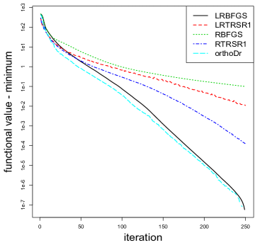
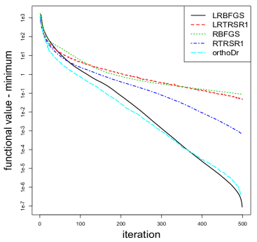
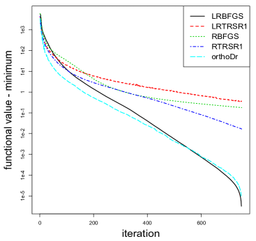
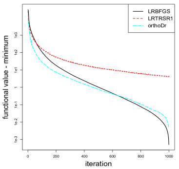
Figure 1: Log of function value vs. iteration ($n=150$)

From left to right, top to bottom: $p=5,10,20$ and 50 respectively.

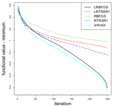
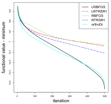
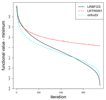
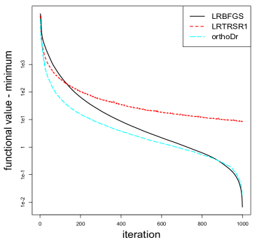
Figure 2: Log of function value vs. iteration ($n=500$)

From left to right, top to bottom: $p=5,10,20$ and 50 respectively.

Table 2: Running times with a fixed number of iterations (in seconds)

$n$	$p$	iteration	ManifoldOpthm				orthoDr
			LRBFGS	LRTRSR1	RBFGS	RTRSR1
$150$	5	250	0.053	0.062	0.451	0.452	0.065
$150$	10	500	0.176	0.201	4.985	5.638	0.221
$150$	20	750	0.526	0.589	28.084	36.142	0.819
$150$	50	1000	2.469	2.662	–	–	6.929
$500$	5	250	0.403	0.414	7.382	7.426	0.423
$500$	10	500	1.234	1.305	57.047	67.738	1.332
$500$	20	750	3.411	3.6	–	–	3.974
$500$	50	1000	13.775	14.43	–	–	19.862

Examples

We use the Concrete Compressive Strength (Yeh, 1998) dataset as an example to further demonstrate the orthoDr_reg function and to visualize the results. The dataset is obtained from the UCI Machine Learning Repository.

Concrete is the most important material in civil engineering. The concrete compressive strength is a highly nonlinear function of age and ingredients. These ingredients include cement, blast furnace slag, fly ash, water, superplasticizer, coarse aggregate, and fine aggregate. In this dataset, we have $n=1030$ observation, 8 quantitative input variables, and 1 quantitative output variable. We present the estimated two directions for structural dimension and further plot the observed data in these two directions. A non-parametric kernel estimation surface is further included to approximate the mean concrete strength.

    R> concrete_data = read.csv(choose.files())    R> X = as.matrix(concrete_data[,1:8])    R> colnames(X) = c("Cement", "Blast Furnace Slag", "Fly Ash", "Water",                "Superplasticizer", "Coarse Aggregate", "Fine Aggregate", "Age")    R> Y = as.matrix(concrete_data[,9])    R> result = orthoDr_reg(X, Y, ndr = 2, method = "sir", maxitr = 1000,     + keep.data = TRUE)    R> rownames(result$B) = colnames(X)    R> result$B                             [,1]         [,2]    Cement             0.08354280 -0.297899899    Blast Furnace Slag 0.27563507  0.320304097    Fly Ash            0.82665328 -0.468889856    Water              0.20738201  0.460314093    Superplasticizer   0.43496780  0.540733516    Coarse Aggregate   0.01141892  0.011870495    Fine Aggregate     0.02936740 -0.004718979    Age                0.02220664 -0.290444936

Figure 3: Response variable over learned directions

Discussion

Using the algorithm proposed by Wen and Yin (2012) for optimization on the Stiefel manifold, we developed the orthoDr package that serves specifically for semi-parametric dimension reductions problems. A variety of dimension reduction models are implemented for censored survival outcome and regression problems. In addition, we implemented parallel computing for numerically appropriate the gradient function. This is particularly useful for semi-parametric estimating equation methods because the objective function usually involves kernel estimations and the gradients are difficult to calculate. Our package can also be used as a general purpose solver and is comparable with existing manifold optimization approaches. However, since the performances of different optimization approaches could be problem dependent, hence, it could be interesting to investigate other choices such as the “LRBFGS” approach in the ManifoldOptim package.

Our package also serves as a platform for future methodology developments along this line of work. For example, we are currently developing a personalized dose-finding model with dimension reduction structure (Zhou and Zhu, 2018). Also, when the number of covariates $p$ is large, the model can be over-parameterized. Hence, applying a $L_{1}$ penalty can force sparsity and allow the model to handle high-dimensional data. To this end, first-order optimization approaches can have advantages over second-order approaches. However, persevering the orthogonality during the Cayley transformation while also preserve the sparsity can be a challenging task and requires new methodologies. Furthermore, tuning parameters can be selected through a cross-validation approach, which can be implemented in the future.

Ruoqing Zhu
Department of Statistics
University of Illinois at Urbana-Champaign
725 S. Wright St., 116 D
Champaign, IL 61820, USA
E-mail: rqzhu@illinois.edu

Jiyang Zhang
Department of Statistics
University of Illinois at Urbana-Champaign
725 S. Wright St.
Champaign, IL 61820, USA
E-mail: jiyangz2@illinois.edu

Ruilin Zhao
School of Engineering and Applied Science
University of Pennsylvania
220 South 33rd St.
Philadelphia, PA 19104, USA
E-mail: rzhao15@seas.upenn.edu

Peng Xu
Departments of Statistics
Columbia University
1255 Amsterdam Avenue
New York, NY 10027, USA
E-mail: px2132@columbia.edu

Wenzhuo Zhou
Department of Statistics
University of Illinois at Urbana-Champaign
725 S. Wright St.
Champaign, IL 61820, USA
E-mail: wenzhuo3@illinois.edu

Xin Zhang
Department of Statistics
Florida State University
214 OSB, 117 N. Woodward Ave.
Tallahassee, FL 32306-4330, USA
E-mail: zhxnzx@gmail.com

References

- Chiaromonte et al. (2002) F. Chiaromonte, R. Cook, and B. Li. Sufficient dimensions reduction in regressions with categorical predictors. The Annals of Statistics, 30(2):475–497, apr 2002. URL https://doi.org/10.1214/aos/1021379862.
- Cook (2009) R. D. Cook. Regression graphics: Ideas for studying regressions through graphics, volume 482. John Wiley & Sons, 2009.
- Cook and Lee (1999) R. D. Cook and H. Lee. Dimension reduction in binary response regression. Journal of the American Statistical Association, 94(448):1187–1200, dec 1999. URL https://doi.org/10.1080/01621459.1999.10473873.
- Cook and Weisberg (1991) R. D. Cook and S. Weisberg. Discussion of ‘sliced inverse regression for dimension reduction’. Journal of the American Statistical Association, 86(414):328, jun 1991. URL https://doi.org/10.2307/2290564.
- Cook and Zhang (2014) R. D. Cook and X. Zhang. Fused estimators of the central subspace in sufficient dimension reduction. Journal of the American Statistical Association, 109(506):815–827, apr 2014. URL https://doi.org/10.1080/01621459.2013.866563.
- Cook et al. (2010) R. D. Cook, B. Li, and F. Chiaromonte. Envelope models for parsimonious and efficient multivariate linear regression. Statistica Sinica, pages 927–960, 2010.
- Dabrowska (1989) D. M. Dabrowska. Uniform consistency of the kernel conditional kaplan-meier estimate. The Annals of Statistics, pages 1157–1167, 1989. URL https://doi.org/10.1214/aos/1176347261.
- Dong and Li (2010) Y. Dong and B. Li. Dimension reduction for non-elliptically distributed predictors: second-order methods. Biometrika, 97(2):279–294, 2010. URL https://doi.org/10.1093/biomet/asq016.
- Eddelbuettel and François (2011) D. Eddelbuettel and R. François. Rcpp: Seamless R and C++ integration. Journal of Statistical Software, 40(8):1–18, 2011. URL https://doi.org/10.18637/jss.v040.i08.
- Eddelbuettel and Sanderson (2014) D. Eddelbuettel and C. Sanderson. Rcpparmadillo: Accelerating r with high-performance c++ linear algebra. Computational Statistics and Data Analysis, 71:1054–1063, March 2014. URL http://dx.doi.org/10.1016/j.csda.2013.02.005.
- Edelman et al. (1998) A. Edelman, T. A. Arias, and S. T. Smith. The geometry of algorithms with orthogonality constraints. SIAM journal on Matrix Analysis and Applications, 20(2):303–353, 1998. URL https://doi.org/10.1137/s0895479895290954.
- Hansen (1982) L. P. Hansen. Large sample properties of generalized method of moments estimators. Econometrica: Journal of the Econometric Society, pages 1029–1054, 1982. URL https://doi.org/10.2307/1912775.
- Huang and Chiang (2017) M.-Y. Huang and C.-T. Chiang. An effective semiparametric estimation approach for the sufficient dimension reduction model. Journal of the American Statistical Association, pages 1–15, 2017. URL https://doi.org/10.1080/01621459.2016.1215987.
- Huang et al. (2018) W. Huang, P.-A. Absil, K. A. Gallivan, and P. Hand. Roptlib: an object-oriented c++ library for optimization on riemannian manifolds. ACM Transactions on Mathematical Software, 44(4):1–21, jul 2018. URL https://doi.org/10.1145/3218822.
- Jolliffe (1986) I. T. Jolliffe. Principal component analysis and factor analysis. In Principal Component Analysis, pages 115–128. Springer New York, 1986. URL https://doi.org/10.1007/978-1-4757-1904-8_7.
- Lee et al. (2013) K.-Y. Lee, B. Li, F. Chiaromonte, et al. A general theory for nonlinear sufficient dimension reduction: Formulation and estimation. The Annals of Statistics, 41(1):221–249, 2013. URL https://doi.org/10.1214/12-aos1071.
- Li and Dong (2009) B. Li and Y. Dong. Dimension reduction for nonelliptically distributed predictors. The Annals of Statistics, pages 1272–1298, 2009. URL https://doi.org/10.1214/08-aos598.
- Li and Wang (2007) B. Li and S. Wang. On directional regression for dimension reduction. Journal of the American Statistical Association, 102(479):997–1008, 2007. URL https://doi.org/10.1198/016214507000000536.
- Li (1991) K.-C. Li. Sliced inverse regression for dimension reduction. Journal of the American Statistical Association, 86(414):316–327, jun 1991. URL https://doi.org/10.2307/2290563.
- Li et al. (1999) K.-C. Li, J.-L. Wang, C.-H. Chen, et al. Dimension reduction for censored regression data. The Annals of Statistics, 27(1):1–23, 1999. URL https://doi.org/10.1214/aos/1018031098.
- Li and Yin (2008) L. Li and X. Yin. Sliced inverse regression with regularizations. Biometrics, 64(1):124–131, 2008. URL https://doi.org/10.1111/j.1541-0420.2007.00836.x.
- Li and Zhang (2017) L. Li and X. Zhang. Parsimonious tensor response regression. Journal of the American Statistical Association, pages 1–16, 2017. URL https://doi.org/10.1080/01621459.2016.1193022.
- Lu and Li (2011) W. Lu and L. Li. Sufficient dimension reduction for censored regressions. Biometrics, 67(2):513–523, 2011. URL https://doi.org/10.1111/j.1541-0420.2010.01490.x.
- Ma and Zhang (2015) Y. Ma and X. Zhang. A validated information criterion to determine the structural dimension in dimension reduction models. Biometrika, 102(2):409–420, 2015. URL https://doi.org/10.1093/biomet/asv004.
- Ma and Zhu (2012a) Y. Ma and L. Zhu. Efficiency loss caused by linearity condition in dimension reduction. Biometrika, 99(1):1–13, 2012a. URL https://doi.org/10.1093/biomet/ass075.
- Ma and Zhu (2012b) Y. Ma and L. Zhu. A semiparametric approach to dimension reduction. Journal of the American Statistical Association, 107(497):168–179, 2012b. URL https://doi.org/10.1080/01621459.2011.646925.
- Ma and Zhu (2013a) Y. Ma and L. Zhu. Efficient estimation in sufficient dimension reduction. Annals of statistics, 41(1):250, 2013a. URL https://doi.org/10.1214/12-aos1072.
- Ma and Zhu (2013b) Y. Ma and L. Zhu. A review on dimension reduction. International Statistical Review, 81(1):134–150, 2013b. URL https://doi.org/10.1111/j.1751-5823.2012.00182.x.
- Martin et al. (2016) S. Martin, A. M. Raim, W. Huang, and K. P. Adragni. Manifoldoptim: An r interface to the roptlib library for riemannian manifold optimization, 2016. URL https://arxiv.org/abs/1612.03930.
- Silverman (1986) B. W. Silverman. Density estimation in action. In Density Estimation for Statistics and Data Analysis, pages 120–158. Springer US, 1986. URL https://doi.org/10.1007/978-1-4899-3324-9_6.
- Sun et al. (2017) Q. Sun, R. Zhu, T. Wang, and D. Zeng. Counting process based dimension reduction methods for censored outcomes, 2017. URL https://arxiv.org/abs/1704.05046.
- Wen and Yin (2012) Z. Wen and W. Yin. A feasible method for optimization with orthogonality constraints. Mathematical Programming, 142(1-2):397–434, aug 2012. URL https://doi.org/10.1007/s10107-012-0584-1.
- Wen et al. (2010) Z. Wen, D. Goldfarb, and W. Yin. Alternating direction augmented lagrangian methods for semidefinite programming. Mathematical Programming Computation, 2(3-4):203–230, 2010. URL https://doi.org/10.1007/s12532-010-0017-1.
- Xia (2007) Y. Xia. A constructive approach to the estimation of dimension reduction directions. The Annals of Statistics, pages 2654–2690, 2007. URL https://doi.org/10.1214/009053607000000352.
- Xia et al. (2002) Y. Xia, H. Tong, W. Li, and L.-X. Zhu. An adaptive estimation of dimension reduction space. Journal of the Royal Statistical Society: Series B (Statistical Methodology), 64(3):363–410, 2002.
- Xia et al. (2010) Y. Xia, D. Zhang, and J. Xu. Dimension reduction and semiparametric estimation of survival models. Journal of the American Statistical Association, 105(489):278–290, 2010. URL https://doi.org/10.1198/jasa.2009.tm09372.
- Xu et al. (2016) K. Xu, W. Guo, M. Xiong, L. Zhu, and L. Jin. An estimating equation approach to dimension reduction for longitudinal data. Biometrika, 103(1):189–203, 2016. URL https://doi.org/10.1093/biomet/asv066.
- Yeh (1998) I.-C. Yeh. Modeling of strength of high-performance concrete using artificial neural networks. Cement and Concrete research, 28(12):1797–1808, 1998. URL https://doi.org/10.1016/s0008-8846(98)00165-3.
- Yin and Cook (2002) X. Yin and R. D. Cook. Dimension reduction for the conditional kth moment in regression. Journal of the Royal Statistical Society: Series B (Statistical Methodology), 64(2):159–175, 2002. URL https://doi.org/10.1111/1467-9868.00330.
- Zeng and Zhu (2010) P. Zeng and Y. Zhu. An integral transform method for estimating the central mean and central subspaces. Journal of Multivariate Analysis, 101(1):271–290, jan 2010. URL https://doi.org/10.1016/j.jmva.2009.08.004.
- Zhao et al. (2017) G. Zhao, Y. Ma, and W. Lu. Efficient estimation for dimension reduction with censored data, 2017. URL https://arxiv.org/abs/1710.05377.
- Zhou and Zhu (2018) W. Zhou and R. Zhu. A dimension reduction framework for personalized dose finding, 2018. URL https://arxiv.org/abs/1802.06156.
- Zhu et al. (2006) L. Zhu, B. Miao, and H. Peng. On sliced inverse regression with high-dimensional covariates. Journal of the American Statistical Association, 101(474):630–643, 2006. URL https://doi.org/10.1198/016214505000001285.
- Zhu et al. (2010a) L. Zhu, T. Wang, L. Zhu, and L. Ferré. Sufficient dimension reduction through discretization-expectation estimation. Biometrika, 97(2):295–304, 2010a. URL https://doi.org/10.1093/biomet/asq018.
- Zhu et al. (2010b) L.-P. Zhu, L.-X. Zhu, and Z.-H. Feng. Dimension reduction in regressions through cumulative slicing estimation. Journal of the American Statistical Association, 105(492):1455–1466, 2010b. URL https://doi.org/10.1198/jasa.2010.tm09666.